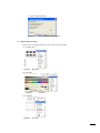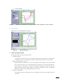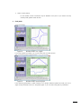
Download IVMAN ver1.2 - Xenosystem Co., Ltd.

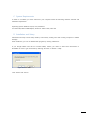
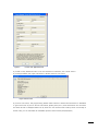
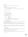
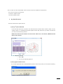
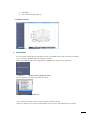
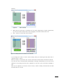
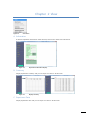
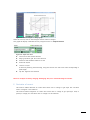
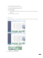
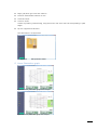
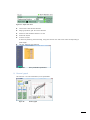
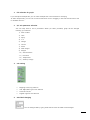
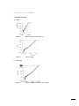
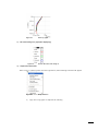
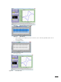
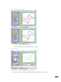
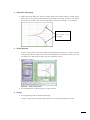
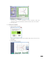
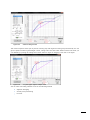
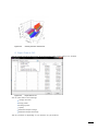
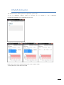
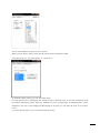
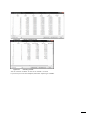
IVMAN ver1.2
User’s Manual
June 2010
T.
+82.31.766.5974
F.
+82.31.765.2645
E.
[email protected]
[email protected]
W.
www.wonatech.com
© 1991–2008 WonATech Co. Ltd.
All rights reserved.
Contents
Overview
.......................................................................................................................................... 1
A. Introduction of IVMan .............................................................................................................................................1
B. What is New in IVMan ............................................................................................................................................1
C. System Requirements ..............................................................................................................................................2
D. Installation and Setup ..............................................................................................................................................2
E. Licensing Note ............................................................................................................................................................4
F. Known Bug ...................................................................................................................................................................4
G. Legal Information.......................................................................................................................................................4
H. END-USER LICENSE AGREEMENT .......................................................................................................................4
I. License Agreement ....................................................................................................................................................4
IVMAN Main program ........................................................................................................................... 6
Chapter １
File .................................................................................................................................... 7
A. Open File .......................................................................................................................................................................7
1.
By data file source .....................................................................................................................................8
2.
File Selection ................................................................................................................................................9
3.
Cycle Selection.......................................................................................................................................... 10
B. Close File .................................................................................................................................................................... 10
C. Convert Rfd to dmf ................................................................................................................................................ 10
D. Save graph as image file ..................................................................................................................................... 12
E. Generate HTML report.......................................................................................................................................... 12
Chapter ２
View ............................................................................................................................... 14
A. Information ................................................................................................................................................................ 14
B. Summary..................................................................................................................................................................... 14
C. Experiment Data ...................................................................................................................................................... 14
Chapter ３
Graph ............................................................................................................................. 16
A. 3D graph .................................................................................................................................................................... 16
1.
Projection .................................................................................................................................................... 16
2.
Autoscale..................................................................................................................................................... 16
3.
Invert Axis ................................................................................................................................................... 17
4.
View direction change ........................................................................................................................... 17
B. V,I,T vs. t ..................................................................................................................................................................... 17
C. I vs. V graph .............................................................................................................................................................. 18
D. Integral of current .................................................................................................................................................. 18
E. Derivative of current .............................................................................................................................................. 19
F. Tafel graph ................................................................................................................................................................ 21
G. Linear Polarization graph..................................................................................................................................... 22
H. General graph........................................................................................................................................................... 23
1.
File selection for graph ......................................................................................................................... 24
2.
X,Y axis parameter selection ............................................................................................................... 24
3.
axis setting ................................................................................................................................................. 24
4.
Axis label changing................................................................................................................................. 24
I. Graph functions in IVMAN.................................................................................................................................. 26
y
Chapter ４
2D Graph function .................................................................................................................................. 26
Analysis ......................................................................................................................... 31
A. Simple Math .............................................................................................................................................................. 31
1.
X-axis for calculation .............................................................................................................................. 31
2.
Y1 axis for calculation............................................................................................................................ 31
3.
Operator selection .................................................................................................................................. 31
4.
Y2 input ....................................................................................................................................................... 31
B. Peak search ............................................................................................................................................................... 32
1.
Peak searching condition ..................................................................................................................... 32
2.
Find peaks .................................................................................................................................................. 33
C. Advanced peak search .......................................................................................................................................... 35
1.
Step1: Choose data set ......................................................................................................................... 35
2.
Step2: Derivative ...................................................................................................................................... 35
3.
Step3: Baseline point ............................................................................................................................. 36
4.
Step4: Peak find ....................................................................................................................................... 36
5.
Step5: Generate Base line .................................................................................................................... 37
6.
Result of peak search ............................................................................................................................ 37
D. Interpolation ............................................................................................................................................................. 38
E. Smoothing ................................................................................................................................................................. 40
1.
Savitzy-Golay smoothing...................................................................................................................... 40
2.
Adjacent averaging ................................................................................................................................. 41
3.
FFT filtering ................................................................................................................................................ 41
F. Differentiation........................................................................................................................................................... 42
G. Integral ........................................................................................................................................................................ 42
H. Semi-Derivative, Integral...................................................................................................................................... 43
I. Tafel analysis ............................................................................................................................................................. 43
1.
Determine tafel region .......................................................................................................................... 44
2.
Initial guessing: ......................................................................................................................................... 44
3.
Fitting ........................................................................................................................................................... 44
4.
Corrosion rate calculation .................................................................................................................... 45
J. Linear Polarization analysis ................................................................................................................................. 46
K. Advanced Integral .................................................................................................................................................. 47
Chapter ５
Example ......................................................................................................................... 49
A. Current density converting ................................................................................................................................. 49
IVMAN differential Analysis ................................................................................................................ 53
A. File Open .................................................................................................................................................................... 53
B. Graph format ............................................................................................................................................................ 53
1.
2D Plot general function ...................................................................................................................... 54
2.
Manual axis range setting ................................................................................................................... 55
3.
Graph option ............................................................................................................................................. 55
C. Measured Data ........................................................................................................................................................ 58
D. Voltage Profile.......................................................................................................................................................... 58
E. Capacity plot ............................................................................................................................................................. 59
F. Differential Analysis................................................................................................................................................ 59
1.
Differential Capacity (EVS) ................................................................................................................... 59
2.
Differential Voltage ................................................................................................................................. 60
3.
Parameters for differential analysis .................................................................................................. 60
4.
3D graph ..................................................................................................................................................... 61
5.
Projection Style......................................................................................................................................... 62
6.
Graph Style................................................................................................................................................. 63
G. Export Data as CVS ................................................................................................................................................ 64
IVMAN Extractor ................................................................................................................................... 66
IVMAN peak find module ................................................................................................................... 69
Overview
A. Introduction of IVMan
IVMan is scientific software for time-voltage-current in DC mode.
This software package consists of IVMAN main program and IVMAN utilities which contains IVMAN
differential analysis, IVMAN extractor and peak searching module
In IVMan main program, you can do analysis with time-voltage-current data set for peak search,
smoothing, tafel analysis including mathematic data treatment etc.
For battery data analysis,
With IVMAN differential analysis function in IVMAN utilities, it can do electrochemical voltage
spectroscopy using charging-discharging data set and display Voltage vs. capacity
With IVMAN extractor, you can divide the cycle file by cycle number or step number.
For voltammogram’s peack searching, simple “peak searching module” may be used.
B. What is New in IVMan
Current IVMan1.1 version can load WonATech product’s data set and BAS(Bioanalytical systems Inc)’s
data set(*.dat). Also It can imported ASCII file set series if they can meet data series condition. These
exiting features will help you manage and analyze your time voltage current data set in a more
productive way than ever before.
x
History
- IVMan 1.0
- Upgrade to IVMan 1.1
- Upgrade to IVMan 1.2
1
C. System Requirements
In order to run IVMan, you must ensure that your computer meets the following minimum software and
hardware requirements.
Operating System: Windows XP, 2K, Vista, Windows7
PC: PentiumIV, RAM: 512MB Display resolution: 1280 x 1024, LAN card.
D. Installation and Setup
Installation and setup can be easily made by continuously clicking “Yes” after running “setup.exe” in IVMan
Package.
After installation, you can run IVMan Main program by clicking “IVMan.exe”
If you bought IVMan and did not activate IVMan, license, you need to send some information to
WonATech in order to get the license by selecting “Activate” on left bar’s “Help”
Figure 1. License Code
Click “send e-mail” button.
2
Figure 2.
License code application form
If you did not buy IVMan and want to test this software for evaluation, click “cancel” button.
If you bought IVMan, then input information in blanks and click “OK” button
Figure 3. Send a mail
If you click “OK” button, The program bring default email software to send these information to WonATech
to get license code. If your PC did not link internet, please paste (ctrl+v) these information into text editor
and send this file to [email protected] by email. You can receive license code by email. Until receipt of
license code, you can use IVMan for WonATech product’s data formats (dmf,rfd,wdf,wif).
3
Figure 4. Notice for 5Minute operation
E. Licensing Note
IVMan license code is available per one PC. You must install IVMan into the PC which you want to use
IVMan software.
F. Known Bug
IVMan uses Microsoft Common Control to open a file, however, the file open dialog is not loaded in some
machines. It is caused from a licensing issue of the ActiveX control. The easiest way to fix it is to install
Microsoft Visual Studio or Visual Basic.
G. Legal Information
Information in this document is subject to change without notice. This document is provided for
informational purposes only and WonATech makes no warranties, either express or implied, in this
document. The entire risk of the use or the results of the use of this document remains with the user.
Without limiting the rights under copyright, no part of this document may be reproduced, stored in or
introduced into a retrieval system, or transmitted in any form or by any means, or for any purpose, without
the express written permission of WonATech
Copyright © 2004-2010 WonATech. All rights reserved.
H. END-USER LICENSE AGREEMENT
Take the time to read this License Agreement prior to installing this software, because by installing the
software, you accept the terms and conditions of this License Agreement. Likewise, if you do not accept
the terms of this agreement, do not install this package.
I.
License Agreement
WonATech Co., Ltd grants you, the purchaser, a non-exclusive license to use the software programs
included in this package. This license is subject to the terms and restrictions set forth in this agreement.
4
You may
Make archival copies of the software programs for the backup purpose only.
You may NOT
Sublicense, rent or lease the software programs.
Modify the program
Reverse engineer, decompile, or disassemble software program or programmable logic
devices.
Use in other PC
Term
This license is effective until terminated.
x
If you have problems
Contact us at your earliest convenience.
We can be contacted via;
E-mail
: [email protected]
Fax
: 82-2-576-2635
Phone
: 82-2-578-6516
Address
: WonATech Co., Ltd
8-6, WooMyun-Dong, SeoCho-Ku, Seoul 137-900, Korea
If you write to us about a problem, provide as much information as possible.
x
Limited Warranty
WonATech Co., Ltd warrants to the original user of this product that it shall be free of defects resulting
from faulty manufacture of the product.
WonATech Co., Ltd makes no warranties regarding either the satisfactory performance of IVMan package
including the software encoded in this product or the fitness of the system for any particular purpose.
WonATech Co., Ltd reserves the right to make revisions to the system at any time without incurring any
obligation to install same on systems previously purchased. All system specifications are subject to change
without notice.
x
Trademarks
Microsoft, Windows, Windows 95, Windows 98, Windows Me, Windows NT, Windows 2000, and Windows
XP Windows Vista are registered trademarks of Microsoft Corporation.
LabVIEW is registered trademark of National Instruments.
Other names of actual companies and product names may be trademarks or registered trademarks of their
respective holders.
5
IVMAN Main program
6
Chapter １ File
Figure 5.
File Menu
A. Open File
In order to open the data file, click “File” on left side menu and select “Open file”
Figure 6.
Select data file to open
A
B
Figure 7.
Main windows structure
7
You can select raw data then IVMan convert this file format into IVMan file format(*.dmf)
You can see 2 section as the above.
“A” section: Graphic section
“B” section: Menu section
1.
By data file source
There are three kind of open data file
１) Using 3rd parties ASCII file
If the data file come from 3rd parties’ ascii file and the file consists series of data in order as timevoltage-current or or Bioanalytical System’s Epsilon format (dat) then Once you select one data file,
you may see the following window.
NOTE: each data must be numeric not text format. If data set is text format, IVMAN will treat
them as note section.
a.
Importing Ascii file
i.
Press “OK”.
ii.
You can see following figure 11
２) Using registered data format
If you open registered data format(WonATech product’s data format, then you can see the following
messege box
Figure 8. Converting file to IVman format
8
a.
Press “OK”.
b.
You can see following figure 11
３) IVMan file format
Figure 9.
2.
After loading data
File Selection
You can upload multiple files by the above process. The loaded data set will be located on memory
so you can select uploaded file(s) by selecting it anytime.
Recent uploaded data file name is displayed at “OPENED FILE” section on left menu bar
Figure 10.
Display of recent uploaded file name
You can see file list by clicking uploaded file name
Figure 11.
Uploaded File list
You can select file name to be activated for graphic and data analysis.
When you select file, you can see graph preview on 3D format at right side(section A)-Figure 8
9
3.
Cycle Selection
If data file contains cycle information (multiple cycle), you can select “all cycle” or any of cycles for
displaying and data analysis
Figure 12.
Cycle selection
B. Close File
If you want close recent open file or active file, select “Close” file in File menu at left side menu bar.
Figure 13.
Confirmation message
C. Convert Rfd to dmf
If you want to convert rfd file(WonATech’s WBCS,WMPG,WPG data file format) to IVMAN data file
format(dmf), select this menu.
Figure 14.
Select data file folder to be converted
You need to select folder which contains rfd data files and click “Current Folder”
Then you can see left side file select section. You can change this folder by clicking “change
10
directory” .
Figure 15.
1.
Select rfd folder
Select rfd file at left side for converting. You can select multiple files. To select multiple files,
you can use ctrl+left mouse button click or dragging or shift+left mouse button click
2.
Click -> button to move files to be converted.
Figure 16. Multiple selection of rfd file to be converted
If you change your mind to convert some rfd file(s) which you located right side, select files to
cancel and click <- button
When you ready to convert files, click “convert” button then rfd files will be converted to dmf files
If you do not want to overwrite them automatically to existing converted files, you can do turn off
“Replace all” by clicking circle lest side of “Replace all”. The color of this circle will be changed to
grey.
After turn off “Replace all” and click “convert” button, if there is already converted file with same
file name then you can see
11
Figure 17.
Overwrite confirmation
D. Save graph as image file
You can convert displayed graph at right side(section1) to jpeg file or bmp file format.
The displayed graph is different by graph menu selection, the converted image file is following this
selection. If there is 3 graph on section1, the convertion will be done 3 times. (Each graph will be
changed separately and have I.D(graph format name) after original file name.)
E. Generate HTML report
You can make report using this function. When you click this function you can see report name
input window.
Figure 18. Report file name input window
Input the file name for report and click OK button then converting process will be done and the
following window will be displayed.
Note: During converting process, You must wait till following display appears.
Figure 19. Report Items selection
1.
Check items by double clicking which you want make your report.
2.
If you want to see report after generating report, check on “open default web browser”
3.
Click “Save” button then report file is generated same as on the above folder and files
name(*.html).
12
Figure 20. Preview of report after saving report file
Figure 21.
Report file Web browser view
13
Chapter ２ View
Figure 22.
View menu
A. Information
If there is experiment information inside data file, This function shows this information.
Figure 23.
Experiment information display
B. Summary
Display experiment summary and you can export this data to excel format
Figure 24.
Display summary
C. Experiment Data
Display experiment data and you can export this data to excel format
14
Figure 25.
Experiment data display
You can see additional data information adding to original data; Semi integral, Integral, Semi
derivative and *th derivative.
Figure 26.
Additional data adding to original data
15
Chapter ３ Graph
Figure 27.
Graph menu
A. 3D graph
You can see 3D graph when you select this mode.
Figure 28. 3D graph
Figure 29. 3D graph menu
1.
Projection
You can check on or check off each parameters to view or not.
2.
z
XY plane
z
YZ plane
z
ZX plane
z
Only projection
Autoscale
This function makes autoscale function enable/disable
z
Xscale
z
Yscale
16
z
3.
4.
Zscale
Invert Axis
z
X-axis
z
Y-axis
z
Z-axis
View direction change
Figure 30.
During dragging
You can change view angle by dragging on graph.
Note: In 3D graph, there is no submenu which describes in general graph function
B. V,I,T vs. t
This graph display 3 graphs versus time.
１) Voltage vs time
２) Current vs. time
３) Temperature vs. time
Figure 31.
V,I,T vs. time graph
Note1): If there is no temperature data, temperature graph is blank.
Note2) Please refer to graph submenu for graphic function
17
C. I vs. V graph
This graph display Current vs. voltage.
Figure 32.
Current vs. Voltage graph
Figure 33. Graph axis menu
z
Format: Axis value format selection
z
Major grid, Minor grid: Grid color selection
z
Precision: Valid numbers selection on axis
z
Autoscale: On/off
z
Loose fit: On/off
If there are peaks by peak searching, using this function axis will fit the scale corresponding to
peak height
z
Flip axis: Opposite axis direction
D. Integral of current
This function makes integration of Current data versus time or voltage to get capacity(vs. time) or
power(vs. voltage). You can select time or voltage at X axis selection.
Figure 34. Current Integral
vs. time graph
18
Figure 35. Current Integral vs. voltage graph
There are two line; One for Semi Integral and the other for Integral.
This graph will display calculated result by integral function on analysis function.
Figure 36. Graph axis menu
z
Format: Axis value format selection
z
Major grid, Minor grid: Grid color selection
z
Precision: Valid numbers selection on axis
z
Autoscale: On/off
z
Loose fit: On/off
If there are peaks by peak searching, using this function axis will fit the scale corresponding to
peak height
z
Flip axis: Opposite axis direction
Note: For analysis of battery charging discharging data, Use “advanced Integral” function.
E. Derivative of current
This function makes derivative of Current data versus time or voltage to get slope. You can select
time or voltage at X axis selection.
This function makes integration of Current data versus time or voltage to get capacity(vs. time) or
power(vs. voltage). You can select time or voltage at X axis selection.
19
Figure 37. Derivative of Current vs. time
Figure 38.
Derivative of current vs. voltage
This graph will display all calculated result by derivative function on analysis function.
If you did 2nd order, 3rd order derivative, the graph will show 2nd order derivative, 3rd order derivative
as the following examples
.
Figure 39.
Figure 40.
Semi derivative, 1 order derivative, 2
st
nd
order derivative, 3rd order derivative vs. time graph
Graph axis menu
20
z
Format: Axis value format selection
z
Major grid, Minor grid: Grid color selection
z
Precision: Valid numbers selection on axis
z
Autoscale: On/off
z
Loose fit: On/off
If there are peaks by peak searching, using this function axis will fit the scale corresponding to
peak height
z
Flip axis: Opposite axis direction
F. Tafel graph
You can see Voltage vs. LogI in tafel graph. This graph will show the result from tafel analysis
together.
z
Figure 41.
Tafel graph before analysis
Figure 42.
Tafel graph after analysis
Figure 43.
Graph axis menu
Format: Axis value format selection
21
z
Major grid, Minor grid: Grid color selection
z
Precision: Valid numbers selection on axis
z
Autoscale: On/off
z
Loose fit: On/off
If there are peaks by peak searching, using this function axis will fit the scale corresponding to peak
height
z
Flip axis: Opposite axis direction
See tafel analysis in analysis menu.
Figure 44.
Tafel parameters viewer
G. Linear Polarization graph
Figure 45. Linear polarization graph before analysis
Figure 46. Linear polarization graph after analysis
22
Figure 47. Graph axis menu
z
Format: Axis value format selection
z
Major grid, Minor grid: Grid color selection
z
Precision: Valid numbers selection on axis
z
Autoscale: On/off
z
Loose fit: On/off
If there are peaks by peak searching, using this function axis will fit the scale corresponding to
peak height
z
Flip axis: Opposite axis direction
Figure 48.
Linear polarization parameters
H. General graph
This function is for user selectable X,Y axis parameters.
Figure 49.
General graph
23
1.
File selection for graph
If you did upload multiple files, you can select multiple files to be activated for overlaying.
To select multiple files, you can use ctrl+left mouse button click or dragging or shift+left mouse button click
in “Available data set”.
2.
X,Y axis parameter selection
You can freely select X and Y parameters. When you select parameter, graph will be changed
following your selection
１) Point number
２) Time
３) Sqrt(t)
４) T^2
５) Voltage
６) Current
７) Power
８) Semi integral
９) Integral
１０) Semi derivative
１１) Derivative
１２) Temperature
１３) Auxiliary voltage
3.
4.
axis setting
9
Mapping: Linear/Log selection
9
Grid: Major/Minor grid color selection
9
Autoscale: On/Off
9
Flipped: Opposite axis direction
Axis label changing
You can change Label by typing inside the box then axis label will be changed.
24
Example) Tafel plot overlay
Select file(s) which you
want overlay
Figure 50.
General graph example
Select Log
Select Voltage
Select
Current
25
I.
Graph functions in IVMAN
y 2D Graph function
１) Zoom
Figure 51.
Mouse dragging area for zoom up
Figure 52.
Zoom up graph
２) Axis scale
Figure 53.
Change maximum axis value by click on value
26
Figure 54.
Zoom up graph
３) File name change on graph(Just displaying)
Figure 55.
Click on file name and change it.
４) Graph internal function
Move cursor to inside of graph and click right button, then following sub menu will appear.
Figure 56.
a)
Graph submenu
Copy data: Copy graph to clipboard as following
27
Figure 57.
b)
Copy data to clipboard
Visible Items
Figure 58.
Visible item menu
b-1) Plot Legend On/Off
Figure 59. Legend on/off
b-2) Scale Legend On/Off
Figure 60. Scale legend
b-3) Graph Pallet
Figure 61. Graph palllet
b-4) Cursor Legend
Figure 62. Cursor legend
28
c)
Export simplified image
Figure 63.
Export simplified image window
５) Side function of Graph
Move cursor to Legend and click on box right side of file name
a) Common plot
Figure 64.
Plot menu
b) Line color
Figure 65.
Line color
c) Line style
Figure 66.
Line style
29
d) Line width
Figure 67.
Line width
e) Bar plot
Figure 68.
Bar plot
f) Interpolation
Figure 69.
interpolation
g) Point Style
Figure 70.
Point style
30
Chapter ４ Analysis
Figure 71.
Analysis menu
A. Simple Math
This function will calculate the data by mathematical rule.
For example if you want blank subtraction, you can you this function.
1.
X-axis for calculation
Select time or voltage on active data set for x-axis
2.
Y1 axis for calculation
Target parameter on active data set to be used for calculation.
3.
Operator selection
You can select +,-,x,/
4.
Y2 input
You can input Y2 value to calculate.
Y2 value may be set as value or formula or external data set.
31
—
Figure 72.
Simple example
10uA offset calculation(Blue line: original, green line: offset value(10uA), red line: calculated)
B. Peak search
This function is for searching peak on graph.
Figure 73.
1.
Peak search window
Peak searching condition
To find proper peak, you must set proper value
¾
Threshold: percent
To generate a proper base line, this module divides the first derivative of current data
among their zeros. For more details, please do "Advanced Peak Search" in main window.
¾
Width: x value width in x axis unit
Width specifies the window size to use in the quadratic least squares fit. The value should
be no more than about 1/2 of the half-width of the peaks and can be much smaller for
noise-free data. Large widths can reduce the apparent amplitude of peaks and shift the
apparent location. Ideally, width should be as small as possible but must be balanced
against the possibility of false peak detection due to noise.
¾
Height: y value percent
This module ignores any peak found with a amplitude that is less than Height above the
base-line.
32
¾
Invert current polarity
In this module, current convention may be different from yours. If you cannot find any
evident peaks, please check this box.
2.
Find peaks
Click “Find peaks”.
Figure 74.
Peak find result in I vs. V graph
If you found peaks successful, you can see result data on Result section.
You can change graph format between I vs V or V,I vs time.
Figure 75.
Peak find result in V,I vs time graph
If the searching parameters in peak condition is not proper, abnormal peak was found, you can readjust some parameters and try to find peaks again or you can edit some peak on peak editor.
33
Figure 76.
Abnormal peak searching result
Figure 77.
Edit peak list
9
Select peaks to be deleted by click on the list (ctrl or shift key pressed). (blue list on
above examples)
9
Click delete button
Figure 78. Peak deleted result
9
Figure 79.
Click apply button
Peak edit result
34
C. Advanced peak search
This function is wizard function to find proper peaks.
1.
2.
Step1: Choose data set
Figure 80.
Advanced peak search front window
Figure 81.
Target parameter selection for peak searching
9
Select data and X axis parameters in time or voltage
9
Click Next
Step2: Derivative
Figure 82.
Smoothing method selection
Selecting Smoothing Method
9
No smoothing
9
Adjacent averaging
9
Savitzky-Golay Smoothing Filter
9
FFT filter
35
3.
Step3: Baseline point
Figure 83.
Baseline point determination
１) Move Threshold bar which you expected
２) Click “find again” button
３) If founded baseline points is not accurate, adjust Threshold value by moving threshold bar
４) Click :find again” button
５) You can “add” and/or “delete” base line point by clicking “add” button and/or “delete”
button after selecting the point left side
６) Each selected point can move by click “move points” button
4.
Step4: Peak find
Figure 84.
Peak find window
１) Select peak width and height
２) Click “find again”
３) If founded peak points is not accurate, adjust width and or height value by moving
threshold bar
４) Click :find again” button
５) You can “add” and/or “delete” peak point by clicking “add” button and/or “delete” button
after selecting the point left side
６) Each selected point can move by click “move points” button
36
5.
Step5: Generate Base line
9
6.
Select base line type
o
Constant
o
Line with slope
o
Line between two ends
Result of peak search
Figure 85.
Result of peak search
You can generate report as html format by pressing “save report” button
37
Figure 86.
Peak find result report output
You can fill peak area by clicking “baseline fill area button”
Figure 87.
Baseline fill area
D. Interpolation
Figure 88.
Interpolation window
38
Figure 89.
Interpolation result using n->8n
Interpolation-(From Wikipedia)
In the mathematical subfield of numerical analysis, interpolation is a method of constructing new data points
within the range of a discrete set of known data points.
In engineering and science one often has a number of data points, as obtained by sampling or experimentation,
and tries to construct a function which closely fits those data points. This is called curve fitting or regression
analysis. Interpolation is a specific case of curve fitting, in which the function must go exactly through the data
points.
A different problem which is closely related to interpolation is the approximation of a complicated function by a
simple function. Suppose we know the function but it is too complex to evaluate efficiently. Then we could pick
a few known data points from the complicated function, creating a lookup table, and try to interpolate those
data points to construct a simpler function. Of course, when using the simple function to calculate new data
points we usually do not receive the same result as when using the original function, but depending on the
problem domain and the interpolation method used the gain in simplicity might offset the error.
It should be mentioned that there is another very different kind of interpolation in mathematics, namely the
"interpolation of operators". The classical results about interpolation of operators are the Riesz-Thorin theorem
and the Marcinkiewicz theorem. There also are many other subsequent results
Definition
From inter meaning between and pole, the points or nodes. Any means of calculating a new point between two
or more existing data points is interpolation.
There are many methods for doing this, many of which involve fitting some sort of function to the data and
evaluating that function at the desired point. This does not exclude other means such as statistical methods of
calculating interpolated data.
One of the simplest forms of interpolation is to take the arithmetic mean of the value of two adjacent points to
find the mid point. This will give the same result as a linear function evaluated at the midpoint.
Given a sequence of n distinct numbers xk called nodes and for each xk a second number yk, we are looking for
a function f so that
A pair xk,yk is called a data point and f is called an interpolant for the data points.
When the numbers yk are given by a known function f, we sometimes write fk.
39
E. Smoothing
Figure 90.
Smoothing window(voltage-current)
You can select graph format in voltage-current or time-voltage & time current or power spectrum.
Figure 91.
1.
Time-voltage/time-current , power spectrum graph for smoothing
Savitzy-Golay smoothing
Input parameters for savitzy-golay smoothing.
Polynominal value, Points to the left, Points to the light
Figure 92.
Savitzky-Golay smoothing
Savitzky–Golay smoothing (From Wikipedia)
The Savitzky–Golay smoothing filter is a type of filter first described in 1964 by Abraham Savitzky and Marcel
J. E. Golay. The Savitzky–Golay method essentially performs a local polynomial regression (of degree k) on a
distribution (of at least k+1 equally spaced points) to determine the smoothed value for each point. Methods
are also provided for calculating the first up to the fifth derivatives.
The main advantage of this approach is that it tends to preserve features of the distribution such as relative
40
maxima, minima and width, which are usually 'flattened' by other adjacent averaging techniques (like moving
averages, for example).
The paper that the filter appeared in is one of the most widely cited papers in the journal Analytical Chemistr]
and is classed by that journal as one of its "10 seminal papers" saying "it can be argued that the dawn of the
computer-controlled analytical instrument can be traced to this article". Savitzky and Golay's original paper
contained several typographical errors that were subsequently corrected by Steinier, Termonia, and Deltour
2.
Adjacent averaging
Figure 93.
Adjacent averaging result
Select the point number for averaging
3.
FFT filtering
Figure 94.
FFT filtering result
41
F. Differentiation
Figure 95.
Differentiation window
１) Select derivative order
２) Select smoothing method after differentiation
３) Click “Differentiation” button
The result will display on the graph as overlay
G. Integral
Figure 96.
Integral window (current vs. voltage graph)
You can calculate internal area by check “calculate internal area”
Also you can see graph type with current vs. voltage or voltage vs.time current vs. time
Figure 97.
Integral window (voltage vs. time ,current vs. time graph)
42
H. Semi-Derivative, Integral
Figure 98.
Semi derivative result
Figure 99.
Semi integral result
１) Select Semi derivative or Semi integral
２) Select smoothing type after Semi derivative or integral
I.
Tafel analysis
Figure 100.
Tafel analysis window
Tafel analysis can get tafel coefficient and corrosion rate.
To get corrosion rate, You must provide equivalent weight and density and active area.
43
1.
Determine tafel region
１) Select data range: Move two points at anodic region and cathodic region to proper points.
IVMan will fit and calculate tafel coefficient using within this region. In order to set anodic
limit point and cathodic limit point for tafel region, click point and drag it to the location.
Click on this point
and
move
it
by
dragging
2.
Initial guessing:
To get a starting point, this module makes initial guessing with linear fit on a part of anodic
and cathodic data set which are extracted with Anodic(%) and Cathodic(%) values. Also you
can select Ecorr value as Ecorr=Eeq or (E,I)corr=Intersection point)
１) Click Initial guessing
Figure 101.
Initial guessing result
２) If initial guessing is not expected, goto 1) step and retry.
3.
Fitting
１) If initial guessing result is satisfied, click fitting.
Fitting on this process is nonlinear least square fit over data set between two cursors.
44
Figure 102.
Fitting result
The fitting result is corrosion potential(Ecorr), Corrosion current(Icorr), Anodic Tafel
coeffient(Ba), Cathodic tafel coefficient(Bc). Polarization resistance value is also calculated.
２) Click “Okay” button
4.
Corrosion rate calculation
１) New input windows will appear
To get corrosion rate(mpy), you must input equivalent weight, density, and active area of
your sample
２) Click “OK” button
You can see result as the follows
Figure 103.
Tafel analysis result
45
J. Linear Polarization analysis
Figure 104. Linear polarization analysis window
１) Select data range: Move two points at anodic region and cathodic region to proper points.
IVMan will fit and calculate polarization resistance using within this region. In order to set
anodic limit point and cathodic limit point for linear polarization region, click point and drag it
to the location.
Click on this point
and
move
it
by
dragging
Figure 105. Select linear data region
２) click “linear fitting”
Figure 106.
Fitting result
46
The fitting result is Polarization resistance.
３) Click “Okay” button
a.
New input windows will appear
Figure 107.
Parameter input
４) Click OK button
５) Linear polarization analysis result will be shown
Figure 108.
Linear polarization analysis result
K. Advanced Integral
This special function is for multiple cycle’s capacity calculation by user setting base line and region. When
you click advanced integral button at left bottom side, you can see following window.
47
Figure 109.
Advanced Integral menu
This function separate each cycle as positive scanning step and negative scanning step automatically. You can
get the peak information (peak height current, voltage value and area value based on base line which you
can defined by inputting the voltage and current value for region or dragging cursor bar to set region.
Figure 110.
1st Cycle’s upper region’s analysis result
You can select smoothing method as one of the following method
y
Adjacent Averaging
y
Savitzky-Golay Smoothing
y
FFT filter
48
Chapter ５ Example
A. Current density converting
Open the data file
Figure 111.
Source data
Figure 112.
Tafel plot with source data
Go to analysis menu and select “simple math”
Figure 113.
Simple Math1
If the sample active area is 3.023cm^2 then input the value as the above
Click “calculate”
Click “apply”
49
Figure 114.
Simple Math2
Then the current data was converted as current density (A/cm^2)
You can see converted data on the graph.
Figure 115.
Tafel plot1 with current density
Graph X-axis label display is still not changed to current density
Click right button of mouse on the location of graph and select “visible items” and check on“scale legend”
Input the characters for x-axis label (example: Current density[A/cm^2]
Figure 116.
Tafel plot2 with current density
Check the current density value. The value was converted as current density as the follows.
50
Figure 117.
Converted data list
51
52
IVMAN differential Analysis
IV differential analysis program is utility program from IVMAN package in order to analysis of battery test
data. This software utility is only for WonATech product’s data format.
To run IV differential analysis, select IV differential analysis on IV untilities or Run "C:\Program
Files\WonATech\IVMANDA\IVMAN Differential Analysis.exe"
A. File Open
Open your rfd or wdf file(This file came from your battery charging/discharging experiment using
WonATech’s WBCS, WMPG, WPG, WEIS instruments)
To do this, click Menu icon.
Figure 118.
IVMAN differential analysis menu
Click “open file” and select battery test data file.
Figure 119.
Menu icon pop up menu
B. Graph format
Using IVMAN differential analysis software, you can see the following graph formats.
y
V,I vs time (Measured Data tab)
y
Specific Capacity vs voltage (Voltage profile tab)
y
Charging Capacity, Discharging capacity vs cycle number (Capacity tab)
y
1/Q0 * dQ/dV vs. voltage (Differential Capacity tab)
y
1/Q0*dV/dQ vs capacity (Differential voltage tab)
53
1.
2D Plot general function
Plots: You can select graph view; “Voltage and current vs. time”, “Capacity vs. cycle number(Capacity)”, “dQ/dV
vs. voltage (Differential capacity)”, “dV/dQ vs. discharging capacity(Differential voltage)
y
Plot Type: Line, Scatter(dot), Line+Scatter
y
Zoom: Drag to select the area for zooming
Figure 120.
y
Zoom up
Rescale to show all: initialize the zoomed plot
54
2.
Manual axis range setting
By clicking the maximum number or Minimum number of each axis, you can input the number to select Max
or Min value of graph view
Figure 121.
3.
Axis value change for manual zooming
Graph option
Click legend then submenu will appear. The menu language will display following our OS language.
Figure 122.
Graph option
Move cursor to graph region and click right button of mouse. The submenu will appear.
55
１) Common plot
Figure 123.
Legend menu
２) Line color
Figure 124.
Line color setting
３) Line style
Figure 125.
Line style setting
４) Line width
Figure 126.
Line width setting
56
５) Bar plot
Figure 127.
Bar plot setting
６) Interpolation
Figure 128.
Interpolartion setting
７) Point Style
Figure 129.
Point style selection
57
Figure 130.
Popup menu on graph region
You can copy the graph into clipboard by selecting “Export Image to Clipboard”
You can paste this graph by “ctrl”+v on your application software such as Excel, Word etc.
C. Measured Data
This tab displays charging/discharging raw data as V, I vs time plot
Figure 131.
V, I vs time plot
This graph is not affected by parameter setting.
D. Voltage Profile
This tab displays specific capacity vs. voltage.
Cycle number setting and Mass value in parameter setting at left side bar will be applied to the graph.
Specific capacity (mAhr/g)=Capacity(mAhr) / Mass (g)
58
Figure 132.
Specific Capacity vs. voltage
E. Capacity plot
This tab displays specific capacity vs. cycle no.
Cycle number setting and Mass value in parameter setting at left side bar will be applied to the graph.
Specific capacity (mAhr/g)=Capacity(mAhr) / Mass (g)
F. Differential Analysis
This analysis mode is to converting data to Differential capacity(dQ/dV vs. voltage) calling EVS
(Electrochemical voltage Spectroscopy) or Differential voltage(dV/dQ vs. specific capacity) graph using battery
charging/discharging data file.
1.
Differential Capacity (EVS)
Differential capacity is the relative change in capacity as a function of the voltage, normalized by the
average BOL C1/25 capacity, QBOL. The C1/25 discharge and charge data are first smoothed, then the
differential capacity is calculated using Equation (1) with a two-point numerical differentiation.
Differential Capacity =1/ Q BOL∗ d(A h)/ dV
To view differential capacity data, click “ differential capacity” tab”
59
Figure 133.
2.
Differential Capacity graph
Differential Voltage
An alternative way of viewing the data is differential voltage, as described in Equation (2).
Differential Voltage = Q BOL∗ dV/ d(A h)
To view differential capacity data, click “ differential voltage” tab”
Figure 134.
3.
Differential Voltage Graph
Parameters for differential analysis
Figure 135.
Parameter setting
You may select averaging function by selecting Pre-Avg.factor and Post-Avg.Factor.(select data point number
for averaging)
60
y
Pre-Avg.factor: Averaging points in raw data
y
Post-Avg.Factor: Averaging points in calculated data
y
You can determine dV value.
y
Q0 value can be input for calculation of 1/Q0
y
Mass value can be defined for specific capacity calculation
(The graph will be changed by selecting averaging and/or dV automatically if you select “Automatic Update”)
If you did not check on “Automatic Update”, you must click “Differential Analysis” button whenever you
change the variables
Figure 136.
Automatic update and cycle selection
You can select cycle number to display graph.
If you want overlay multiple cycles data, click the cycle number with pressing “ctrl” key or ”shift” key for
ranged selection
4.
3D graph
You can see 3D graph for differential data display or Voltage profile plot by clicking 3D graph.
Figure 137.
3D graph
61
１) Plane Projection
Figure 138.
3D graph show menu
You can select plane projection in Show option.
5.
Projection Style
Figure 139.
Projection style
There is two type depending on projection style (orthographic or perspective)
Figure 140.
3D plot (orthographic style)
62
Figure 141.
3D plot(perspective style)
Version 2.2 does not provide surface plot which have provided in previous versions.
You can change the view angle by dragging on the graph
Figure 142.
6.
View angle change(Left: orthographic, Right perspective)
Graph Style
Curve plot
This graph style displays plot as indivisual plot. Line and dot for each data set is available.
Surface plot
You can show 3D plot with surface.
Figure 143.
Surface plot option
63
Figure 144.
Surface plot with “surface+line”
G. Export Data as CVS
You can convert the file as ascii format. To do this function, select “export data as cvs” in Menu.
Figure 145.
Export data as cvs
You can select data in the followings
y Voltage & current
y Charge profile
y Discharge profile
y Capacity
y Differential analysis-Charge
y Differential analysis-discharge
This file conversion is depending on your selection of cycle numbers.
64
65
IVMAN Extractor
This software function makes cycle data as splitted by cycle or step.
To
run
IV
differential
analysis,
select
IV
extractors
on
IV
untilities
or
Run
"C:\Program
Files\WonATech\IVMAN extractor\IVMAN extractor.exe"
To open the source file, click Open button and select the file.
Break down criteria can be selected among cycle,, cycle & step or index.
To save splitted files, select Export ASCII tab.
66
You can select delimiter by space or tab or comma.
When you click “export” button, each ascii file will be saved on destination folder.
Using special tab, you can make capacity vs. voltage data.
To generate specific capacity, you can input Mass value.
Pre cycle selection is for discharging data analysis. Except of selected cycles as pre cycle, unselected cycles
will display discharging capacity data only. Selected pre cycles, charging data & discharging data will be
displayed. If you want to see charging and discharging for all cycles, you can select all cycles as pre cycle by
ctrl+A
If you click Preview button, you can see the following window
67
Figure 146.
Capacity profile preview
Figure 147.
Summary preview
You can save this contents as ascii file or transfer it to Excel.
If you have your own excel template, Automatic reporting is available.
68
IVMAN peak find module
This IVMAN utility is to find peaks on voltammogram simply.
To run IV differential analysis, select IV differential analysis on IV untilities or Run "C:\Program
Files\WonATech\IVMANpfm\IVMAN peak find module.exe"
Figure 148.
IVMAN peak find module
By clicking “open” button, you can select data file.
Figure 149.
Zone selection to detect peak etc.
To change searching parameter, select parameters tab.
69
Figure 150.
Parameters setting
Figure 151.
Peak finding result
70