Download 6 Degree of Freedom Splash Pattern Generation Tool

6 Degree of Freedom Splash
Pattern Generation Tool
Release: 1.1.0
©2002
Hall Consulting
320 W. Felspar Ave.
Ridgecrest, CA 93555
http://splashpattern.com
Forward
While the general layout and presentation of knowledge in this text is such that the user may read
it "cover to cover," the author doubts that many users endeavor to do so. Rather, it is expected that this text
will primarily be used as reference. As a result of this assumption the style of this text is rather stilted; it is
often short and sweet to a nearly excessive degree. The text also repeats itself in several places as it was
judged that redundancy of information was preferable to forcing the user to flip through several sections of
the User's Manual just to perform or understand one facet of the simulation's operation or use.
That said, this is also a convenient time and place for me to acknowledge those who have
influenced me in ways that either made this work happen or made my job easier. I would like to thank the
following individuals for their encouragement, knowledge, help, and/or inspiration as appropriate:
Mr. Ed Brown
Mr. Ray Calkins
Mr. David McCue
Mr. Tom Rouse
Dr. Ned Smith
Mr. Rick Wills
2
Table of Contents
INTRODUCTION .........................................................................................................................................4
WHAT SPLASH IS ..........................................................................................................................................5
WHAT SPLASH ISN’T .....................................................................................................................................6
MODELS .......................................................................................................................................................7
Earth........................................................................................................................................................7
Atmosphere..............................................................................................................................................7
Vehicle.....................................................................................................................................................7
INSTALLATION ...........................................................................................................................................10
THE GUI APPLICATION .........................................................................................................................11
MAIN WINDOW ..........................................................................................................................................12
INPUT WINDOWS ........................................................................................................................................12
Launch Site............................................................................................................................................12
Uncertainties .........................................................................................................................................14
Aerodynamics ........................................................................................................................................16
Fins........................................................................................................................................................17
Geometry/Mass......................................................................................................................................18
Propulsion .............................................................................................................................................19
Staging/Recovery...................................................................................................................................22
RUNNING THE SIMULATION ........................................................................................................................24
OUTPUT ......................................................................................................................................................25
Splash Pattern Files/Window ................................................................................................................25
Trajectory Data Files/Window ..............................................................................................................27
THE CONSOLE APPLICATION .............................................................................................................29
DESCRIPTION ..............................................................................................................................................30
INPUT REQUIREMENTS ...............................................................................................................................30
General Input Conventions....................................................................................................................30
Scenario Files........................................................................................................................................31
Stage Files .............................................................................................................................................34
Staging and Recovery Criterion Explained ...........................................................................................43
EXECUTION ................................................................................................................................................45
OUTPUT ......................................................................................................................................................45
Screen Output ........................................................................................................................................45
Splash Pattern File................................................................................................................................46
Trajectory Files .....................................................................................................................................47
APPENDICES .............................................................................................................................................49
TIPS AND TRICKS........................................................................................................................................50
KNOWN BUGS ............................................................................................................................................51
NEW FEATURES & BUG FIXES....................................................................................................................52
SOFTWARE LICENSE ...................................................................................................................................53
ABOUT THE AUTHOR ..................................................................................................................................54
GLOSSARY..................................................................................................................................................55
INDEX .........................................................................................................................................................56
3
Introduction
4
What Splash is
Splash is a wind-weighted 6 degree-of-freedom (6DOF) rocket simulation with statistics-based
impact analysis capability. Splash is intended not just for the nominal trajectory analysis that most
simulations are, but also for splash pattern generation consistent FAA/OST requirements. This means that
Splash can provide the data used to determine not just a nominal impact point but an impact zone complete
with statistics to back up the likelihood of a vehicle impact in any given region. No other simulation
package available at a reasonable price1 offers this capability.
Splash provides more capability and tracks more variables than other consumer-level simulation
packages (and thus, provide data that comes closer to matching reality) available today. Splash’s features
include:
•
•
•
•
•
•
Wind effects (weather cocking).
Earth modeled as a rotating oblate spheroid.
Gravitational effects that vary with altitude and latitude.
An altitude model that extends to 632 km above sea level (ASL).
Clustering of up to 5 motors per vehicle stage.
Uncertainty analysis for 18 different vehicle/scenario parameters.
To better illustrate what all this means, imagine your typical rocket simulation. The simulation
will say that the rocket goes up and comes down in a certain location. Question: What are the odds that the
actual rocket would impact the exact location specified? Answer: About zero. So how close to the
simulation specified location can you expect your rocket to land? Most simulations will provide no insight
as to the answer of that second question. Splash provides a realistic idea of where the rocket might land.
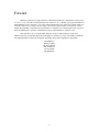
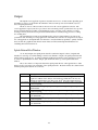
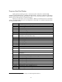
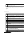
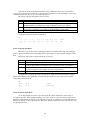
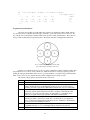
A splash pattern representing 250 possible impact points.
The launch point is designated by the red circle on the right.
The figure above is a plot listing 250 potential impact points of a particular rocket. The
distribution of the impact points illustrates not just a nominal impact point, but provides a level of
confidence with respect to the likelihood of an impact in any given region. Such data is indispensable in
pre-launch safety analysis and is also of use in determining possible locations for wayward rockets. It is
this capability that sets Splash apart.
1
The author is prepared to retract this statement the moment he is made aware of another simulation
package of similar capability and price is made known to it.
5
What Splash isn’t
First and foremost, Splash is not a modeling package. In the eyes of the general public, there is no
perceived no difference between modeling and simulation. There is, however, a difference. Modeling
involves the determination of static performance parameters. For rockets, this means things such as drag
coefficients, mass properties, etc. In contrast, simulation involves putting models in motion in the context
of set timelines and scenarios. In lay terms, models may be thought of as the input for simulations2.
Beware: Splash does not determine drag coefficients, mass properties, thrust curves, or any other
performance parameter. These parameters are instead required as input from the user. The user may obtain
such data from other programs3, hand calculations, actual test data, a Ouija board, or any other means the
user deems up to the task. Splash “merely” integrates the performance data and puts it in motion.
Thus, the user will be required to independently provide the following data for each stage (in no
particular order):
•
•
•
•
•
•
•
Gross vehicle geometric properties
o Length
o Nominal diameter (and thus, frontal area)
Mass properties
o Mass
o Center of gravity as a function of mass
o Moments of inertia at launch
o Products of inertia at launch
Aerodynamic properties
o Ca as a function of Mach and AOA
o Cb as a function of Mach and angle of attack (AOA)
o Cn as a function of Mach and AOA
o CP as a function of Mach and AOA
Fin information
o Location, number and dimensions
Propulsion system
o Thrust/time curve
o Propellant mass
o Sea level total impulse
o Nozzle exit area
Recovery system
o Conditions of deployment
o Diameter
o Sub-sonic drag coefficient
Current launch site conditions
o Longitude, latitude, and altitude
o Barometric pressure and temperature
o Wind speed and direction as a function of altitude
2
This is not entirely true, but it is close enough for the purposes of this discussion.
Examples of such programs include but are not limited to: ADAM, AeroCFD, AP98, DATCOM,
HyperCFD, PEP, RockSim, and Zeus.
3
6
Models
Earth
The Earth model employed by Splash is based on the WGS-844 Earth model. Splash models the
Earth as perfectly smooth, rotating spheroid of uniform density. The primary parameters of this model are
as follows:
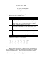
Major Axis (m)
Minor Axis (m)
Average Radius (m)
Angular Velocity (rad/s)
Mass (kg)
Mass * Gravitational constant (m3/s2)
“Standard” Gravitational Acceleration (m/s2)
6378137.0
6356752.3
6371008.7
72.92115e-6
5.979e24
3.986004418e14
9.80665
Note that from the perspective of a fixed, Earth-centered coordinate system, gravitational
acceleration is assumed to be strictly a function of distance to the center of the Earth. But this is only part
of the story. The fact that the Earth is non-spherical coupled with its rotation yields a more complex
gravitational model when by an observer on the Earth’s surface. The result is that gravitational acceleration
as seen by an observer on the Earth’s surface varies not only with altitude (as one would expect) but also
with latitude (as one may not expect).
Atmosphere
Two different atmospheric models are used by Splash. The first model, used for density altitude
correction initialization defines atmospheric conditions as the inverse of a 5th order polynomial. The other
model produces data that matches the ISO 1978 standard atmosphere to an altitude of 631 km above sea
level and is used by Splash at all times during flight modeling.
Vehicle
The vehicle(s) modeled by Splash are assumed to be perfectly rigid, axisymmetric bodies of up to
3 stages. The specific aspects of the vehicle model have been broken down into more logical, more
manageable pieces: mass properties, aerodynamics, and propulsion.
Mass Properties
The mass properties tracked by Splash are as follows: length, nominal diameter, mass, center of
gravity, and the moments and products of inertia. Length, diameter, and mass are obviously
straightforward in nature; the center of gravity as well as the moments and products of inertia do warrant
additional discussion, however.
The center of gravity is assumed to lie on the vehicle’s axis of symmetry. It does, however, move
fore and aft as a function of mass as defined by the user.
4
. For those not familiar with the WGS-84 model, it is the primary Earth model employed by the Global
Positioning Satellite (GPS) system. For more information, see “Department of Defense World Geodetic
System 1984”, National Imagery and Mapping Agency (NIMA) document number NIMA TR8350.2. This
document is available to the public for download at http://www.nima.mil.
7
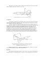
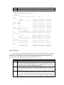
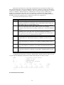
The vehicle’s local coordinate system is centered about the current center of mass and orientated
similar to industry standard (X = forward, Y = port, Z = up).
A sketch illustrating the local vehicle coordinate system.
Aerodynamics
Given Splash’s assumption of an axisymmetric vehicle, it logically follows that the aerodynamic
assumptions used by Splash are axisymmetric as well. This means that current roll angle does not affect
axial or normal forces at non-zero angles of attack.
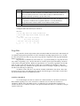
One aspect of Splash’s aerodynamic model that may throw many users off balance is the use of
axial and normal aerodynamic forces rather than the lift and drag forces most people are familiar with. Lift
and drag forces are respectively defined to be perpendicular and opposite to the velocity vector. By
contrast, normal and axial forces are defined as perpendicular and opposite to the vehicle’s own
longitudinal axis. Both systems are valid. Both systems provide for vector addition that yields the net
aerodynamic forces acting upon the vehicle. But to understand why the axial/normal force pairing is
advantageous for rocketry work one need only remember that the vast majority of hobby rocketry
accelerometers are one-dimensional; they record accelerations in-line with the vehicle longitudinal axis.
As a result the data processing required to properly interpret data from such instrumentation is reduced.
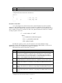
A sketch illustrating the relationships between lift, drag, normal and
axial forces and their orientations with respect to the vehicle’s
longitudinal axis and velocity vector.
Splash models the axial force, normal force, and center of pressure as a family of second order
polynomials that are functions of angle of attack and Mach number.
Propulsion
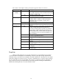
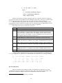
Each stage modeled by Splash is assumed to possess a cluster of up to 5 motors. The engines are
arranged in a cluster as seen in the picture below. Obviously, not every stage has 5 motors; most, in fact
8
will not. For stages with fewer than 5 motors, the motors that do not exist in reality are simply simulated as
motors that produce zero thrust and consume zero fuel.
The methodology used to describe any single motor is based upon proven methodologies used in
government laboratories to model rocket motors within the context of kinematic analysis codes. While
these methodologies assume constant specific impulse throughout the motor’s burn, they do provide thrust
corrections associated with the local ambient atmospheric pressure. The input requirements for these
methodologies is as follows:
•
•
•
•
Total impulse at sea level (N*s).
Propellant mass (kg)
Nozzle exit area (m^2)
Time/Thrust curve (s, N)
9
Installation
Assuming a system capable of running Splash5, installation of Splash is trivial. The distribution
disk is set up to automatically launch the installation routine upon insertion into the disk drive. If for any
reason the installation routine should fail to automatically start up, the user may manually start the routine.
The installation routine is found in the distribution disk's root directory and is called "installer.exe."
Installer handles everything associated with Splash installation with minimal input required of the user.
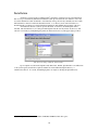
At installation, the user is asked to provide the name of a directory in which Splash will be
installed. The default directory is “C:\Program Files\Splash” but the user may dictate any directory that
suites his or her fancy by manipulating the pull-down menus and text box (at the upper right) provided.
The directory dialog within the install routine.
Upon completion of the install, Splash is fully functional. Further, Splash makes no modifications
to the system registry and all files required at runtime are found within the Splash directory or
subdirectories thereof. As a result, uninstalling Splash is as simple as deleting the Splash directory.
5
System requirements: Win95+, Pentium, CD-ROM, 10 MB free hard drive space.
10
The GUI Application
11
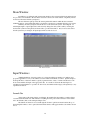
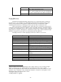
Main Window
In addition to providing the pull-down menus that drive all user-input in Splash, the main window
also provides some feedback to the user in the status bar at the bottom of the window. Of primary interest
are the base file name and unit system panes.
The base file name pane provides the current path and file name in which the data contained
within the memory of the Splash GUI will be saved in the event the user commands Splash to save its data.
Similarly, the unit system pane informs the user of the current unit system - SI or English - for
which input/output is expected/presented. The user may change the unit system at will by selecting the
desired unit system from the pull-down menu at the top of the main window. Note, however, that before
the unit system may be changed, all input/output windows must be closed.
The main window.
Input Windows
A 6DOF simulation obviously requires a lot of data describing any number of conditions and
properties applicable not only to the vehicle, but to the launch environment as a whole. Splash attempts to
break up this mass of data into smaller, logically organized blocks of data. A window dedicated to each
block of data handles the input of the appropriate data. As a result it is believed that data input is as
straightforward and intuitive as possible. In other words, the GUI should be largely self-explanatory to any
experienced rocketeer.
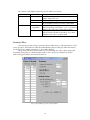
Launch Site
As the name of this input window would imply, the Launch Site input window contains all data
concerned with the launch site. This includes everything from the position and orientation of the launch
rail to the altitude (ASL) of the anticipated impact zone.
The launch site window is accessed through the “Scenario” pull-down menu found at the top of
the main Splash window. Once opened, the Launch Site window will appear similar to the window shown
below.
12
The Launch Site input window.
The contents of each input box in the launch site window is as follows:
Classification
Wind
Column/Box
Altitude
Direction
Atmosphere
Speed
Temperature
Pressure
Location
Longitude
Latitude
Description
The altitude (m or ft, ASL) for which the wind data
(direction and speed) in the next columns is valid.
The direction (degrees) from which the wind is
originating. An angle of zero degrees defines a wind
from the North; an angle of 90 degrees defines a wind
from the East, etceteras.
The speed (m/s or ft/s) at which the wind is blowing.
The ambient temperature (deg C or F) at the launch site.
This data is used to determine the local air density and
thus the correct density altitude. It is not, however, used
to modify local sonic conditions.
The barometric pressure (mmHg or inHg) at the launch
site. This data is used to determine the local air density
and thus the correct density altitude. If the current
barometric pressure is unknown or if the user simply
wishes to use a standard atmosphere, a negative value in
this block will turn off atmospheric corrections.
The longitude (in the WGS-84 coordinate system) of
rocket’s center of gravity at the start of the simulation.
East longitude is defined as a positive angle while West
longitude is defined as a negative angle.
The latitude (in the WGS-84 coordinate system) of
rocket’s center of gravity at the start of the simulation.
North latitude is defined as a positive angle while South
latitude is defined as a negative angle.
13
Altitude
Rail Data
Azimuth
Elevation
Length
Impact Zone
Altitude
The altitude (m or ft, ASL in the WGS-84 coordinate
system) of the rocket’s center of gravity at the start of the
simulation.
The azimuth angle (degrees) in which the launch rail (and
rocket) is pointing at the start of the simulation. An
angle of zero degrees defines a rail pointing to the North;
an angle of 90 degrees defines a rail pointing to the East,
etceteras.
The elevation angle (degrees) in which the launch rail
(and rocket) is pointing at the start of the simulation. An
angle of -90 degrees defines a rail pointing straight up; an
angle of 0 degrees defines a horizontal launch rail.
The distance (m or ft) the vehicle must travel before it is
released from the launch rail.
The altitude (m or ft, ASL) of the impact zone's terrain
.
Most of the time this will be the same as the launch rail
altitude, but not always. An obvious exception to this
rule would be an air-launched system.
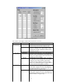
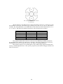
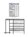
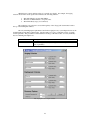
Uncertainties
The primary purpose of Splash is to generate splash patterns for sounding rockets. Obviously, one
must possess a working knowledge of the uncertainties associated with any given vehicle and launch
scenario. The Uncertainties input window defines these uncertainties.
The Uncertainties window is accessed through the “Scenario” pull-down menu found at the top of
the main Splash window. Once opened, the Uncertainties window will appear similar to the window
shown below.
The Uncertainties input window.
14
The contents of each input box in the uncertainties window is as follows:
Classification
Iterations
Column/Box
Mass Properties
Mass
Aerodynamics
Moments of
Inertia
Center of
Gravity
Ca
Cn
CP
Fin Cant
Propulsion
Total Impulse
Propellant
Thrust Axis
Wind
Direction
Velocity
Launch Rail
Azimuth
Elevation
Failure
Ignition
CATO
Deployment
Chute Failure
Description
The number of iterations one desires to run for the given
scenario. It is recommended that the user start with a
small number (5-10) to see if the simulation has any
obvious problems before committing oneself to a splash
pattern generation (a task that can take many hours to
complete). The number of iterations required for splash
pattern generation will vary depending upon the
complexities of the mission and the needs of the user.
Realistic iteration values range anywhere from 100 to
30,000.
The single standard deviation uncertainty in launch mass
expressed as a percentage.
The single standard deviation uncertainty in moments
and products of inertia expressed as a percentage.
The single standard deviation uncertainty in center of
gravity in calibers.
The single standard deviation uncertainty in axial force
coefficient expressed as a percentage.
The single standard deviation uncertainty in normal force
coefficient expressed as a percentage.
The single standard deviation uncertainty in center of
pressure in calibers.
The single standard deviation uncertainty in fin cant
angle in degrees.
The single standard deviation uncertainty in total impulse
expressed as a percentage.
The single standard deviation uncertainty in propellant
mass expressed as a percentage.
The single standard deviation uncertainty in thrust
alignment in degrees.
The single standard deviation uncertainty in wind origin
direction in degrees.
The single standard deviation uncertainty in wind speed
in meters or feet per second.
The single standard deviation uncertainty in launch rail
azimuth angle in degrees.
The single standard deviation uncertainty in launch rail
elevation angle in degrees.
The likelihood of single motor ignition failure expressed
as a percentage.
The likelihood of single motor catastrophic failure
expressed as a percentage. Note that all CATOs are
assumed to occur at motor ignition.
The likelihood of recovery system deployment failure
expressed as a percentage.
The likelihood of recovery system failure expressed as a
percentage.
15
Aerodynamics
As the name of this input window may imply, the Aerodynamics input window contains data
concerned with gross vehicle aerodynamics.
The Aerodynamics window is accessed through any of the “Vehicle->Stage” pull-down menus
found at the top of the main Splash window. Once opened, a Aerodynamics window will appear similar to
the window shown below.
The Aerodynamics input window.
The contents of each input box in the aerodynamics window is as follows:
Classification
Mach
Ca
Column/Box
Multiplier
Ca
dCa
Cb
Description
The axial force multiplier. This is simply a constant by
which the nominal axial force coefficient is multiplied by
to facilitate drag sensitivity studies. Normally, the
associated value will be 1.0, but suppose the user wishes
to model a 10% drag increase. In which case, the user
would merely have to use an axial force multiplier of 1.1
rather than re-calculate and re-type the entire axial force
coefficient table.
The zero angle of attack axial force coefficient.
The derivative of the axial force coefficient with respect
to angle of attack.
The base drag coefficient. The user should ensure that
the base drag coefficient is used; many aeroprediction
codes list the base pressure coefficient. The two
coefficients are related, but not equivalent.
16
Cn
Multiplier
Cn
dCn
CP
Offset
CP
dCP
The normal force multiplier. This is simply a constant by
which the nominal normal force coefficient is multiplied
by to facilitate normal force sensitivity studies.
Normally, the associated value will be 1.0, but suppose
the user wishes to model a 10% lift increase. In which
case, the user would merely have to use a normal force
multiplier of 1.1 rather than re-calculate and re-type the
entire normal force coefficient table.
The zero angle of attack normal force coefficient (usually
zero).
The derivative of the normal force coefficient with
respect to angle of attack.
The center of pressure offset. The offset is simply a
constant that is added to the nominal CP to facilitate
stability sensitivity studies. Normally, the associated
value will be 0.0, but suppose the user wishes to model a
CP shifted one caliber forward. In this case, the user
would use a CP offset of -1.0 rather than re-calculate and
re-type the entire center of pressure table.
The zero angle of attack center of pressure (in calibers).
The derivative of the center of pressure with respect to
angle of attack.
Fins
As the name of this input window implies, the Fins input window contains data concerned with
fins. It should be prominently noted that Splash only uses fin data for yaw/pitch/roll damping. Fin data
does not affect lift, drag, or stability in the normal sense; the effects of fins on these vehicle attributes are
expected to have been included in the gross vehicle aerodynamics.
The Fins window is accessed through any of the “Vehicle->Stage” pull-down menus found at the
top of the main Splash window. Once opened, a Fins window will appear similar to the window shown
below.
The Fin input window.
17
The contents of each input box in the fin properties window is as follows:
Classification
General Info
Column/Box
Number of fins
Cant angle
Area of 1 fin
Location
Fin CP,
longitudinal
Fin CP, radial
Description
The number of fins possessed by the rocket. Valid
numbers range from 3 to 6.
The fin cant angle in degrees.
The area of one side of one fin expressed as a multiple of
the aerodynamic reference area for the overall vehicle.
The longitudinal center of pressure of a fin, measured in
calibers from the tip of the vehicle's nose. A good rule of
thumb for this value is the ¼ chord mark on the fin.
The radial center of pressure of a fin, measured in
calibers from the centerline of the vehicle. A good rule
of thumb for this value is ½ caliber added
Geometry/Mass
Obviously, the geometry and mass properties window defines the gross vehicle dimensions as well
as mass properties. It should be noted that the nominal diameter entered on this page defines the reference
area used for all aerodynamic calculations; i.e. Aref = PI/4 * Diam^2.
The geometry and mass properties window is accessed through any of the “Vehicle->Stage” pulldown menus found at the top of the main Splash window. Once opened, a geometry/mass properties
window will appear similar to the window shown below.
The geometry/mass properties input window.
18
The contents of each input box in the geometry/mass properties window is as follows:
Classification
Center of
Gravity
Column/Box
Mass
CG
Geometry
Launch Mass
Inertial Tensor
Diameter
Length
Mass
Ixx
Ixy
Ixz
Iyy
Iyz
Izz
Description
The mass (kg or lbm) associated with the CG listed in the
next column. At least two masses should be listed and all
should be ascending order.
The center of gravity (calibers) that corresponds to the
mass listed in the previous column.
The nominal diameter of the vehicle (m or ft). This
parameter defines "1 caliber" as well as the reference
area used for most aerodynamic constants (Aref =
PI*Diameter^2/4).
The nominal length of the vehicle (calibers).
The initial mass (kg or lbm) of the stage or vehicle in
question.
The mass (kg or lbm) corresponding to the moments and
products of inertia that make up the inertial tensor.
Obviously, moments/products of inertia vary with mass.
Splash assumes a linear relationship between the mass
and moments/products of inertia. This is not always the
best assumption, but it is reasonable and simplifies user
input requirements.
The moment of inertia (kg*m^2 or lbm*ft^2) taken about
the X axis (longitudinal/"forward").
The product of inertia (kg*m^2 or lbm*ft^2) taken in the
XY plane.
The product of inertia (kg*m^2 or lbm*ft^2) taken in the
XZ plane.
The moment of inertia (kg*m^2 or lbm*ft^2) taken about
the Y axis ("port").
The product of inertia (kg*m^2 or lbm*ft^2) taken about
the YZ plane.
The moment of inertia (kg*m^2 or lbm*ft^2) taken about
the Z axis ("up").
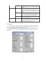
Propulsion
While providing perhaps the most obviously needed data in a rocket simulation, the propulsion
system input window is visually the most intimidating. It really is quite simple though. Splash models
each stage as if it possessed five motors arranged as seen in the sketch below. Obviously, not every vehicle
in the real world has five rocket motors in it - most have considerably fewer. To allow for this fact, Splash
does not require that every motor provide thrust, have a nozzle, or even have any mass for that matter. In
other words, motors that are not found in the real-world vehicle Splash is modeling are mathematically
nullified, thus ensuring that they do not affect simulation results.
19
The configuration of all five motors
in each stage.
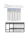
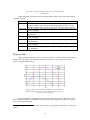
All these null motors may make the user wonder why include provisions for so many motors given
the fact that the vast majority of the vehicle stages out there possess only one or two motors. The answer is
versatility. By varying which motors are nullified the user may effectively model balanced clusters of 1, 2,
3, 4, or 5 motors. The table below illustrates in detail how various clusters may be modeled.
Motors in Cluster
0
1
2
3
4
5
Active Motors
1
2,3
1,2,3
2,3,4,5
1,2,3,4,5
Null Motors
1,2,3,4,5
2,3,4,5
1,4,5
4,5
1
-
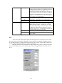
The propulsion window allows the user to select any of 167 different pre-defined (commercial)
motors ranging from C impulse to N. However, by selecting a "custom" motor the user is also allowed to
define his/her own motors. Custom motors have no size, thrust, or burn length limitations.
The propulsion window is accessed through any of the “Vehicle->Stage” pull-down menus found
at the top of the main Splash window. Once opened, a propulsion system window will appear similar to the
window shown below.
20
The propulsion system input window
displaying data for motor #1.
The contents of each input box in the propulsion system window is as follows:
Classification
Motor X (1-5)
Column/Box
Ign Delay
Location
File
Total Impulse
Prop Mass
Nozzle
Description
The delay (seconds) from the activation of the current
stage until the ignition of the motor in question. In most
cases, the ignition delay will be zero. Non-zero numbers
are, however, desired in the event of air-started motors or
multiple stage rockets with coast periods between stage
separations and ignitions.
The motor’s off-centerline distance (m or ft) in
accordance with the motor configuration sketch seen
previously in this section of the manual6. Being on the
centerline by definition, motor 1 will always have an offcenterline distance of 0.0. The rest of the motors should
obviously have non-zero offset distances.
The file that contains pre-programmed motor data for the
motor in question. Performance data for custom motors
is loaded or saved as appropriate to or from the listed file
when the load/save buttons are clicked.
The sea-level total impulse (N*s or lbf*s) of the motor in
question.
The mass of propellant (kg or lbm) contained within the
motor in question.
The total exit area of all nozzles (cm^2 or in^2)
possessed by the motor in question.
6
Note that the number 1 motor is assumed to be on the vehicle’s center line and thus the off-centerline
distance is always zero.
21
Time
Thrust
The data that defines the time axis on the thrust/time
curve. Time is measured in seconds.
The data that defines the thrust axis on the thrust/time
curve. Units are unimportant as the curve will ultimately
be scaled to match the previously defined total impulse.
Staging/Recovery
The manner in which Splash handles staging and recovery system deployment is probably the
most unique piece of programming logic within Splash. Rather than simply staging/deploying by time,
altitude, or body elevation as many systems do, Splash allows the user to construct more complex
staging/deployment criterion by combining up to three logical tests that are evaluated in series7.
Each test performed for staging/deployment contains three pieces of information. The first piece
of information is the flight parameter for which the testing is dependent. Examples of the flight parameter
are altitude, time, and dynamic pressure. The second piece of information is a numerical value to which the
flight parameter is compared. The final piece of information is simply a flag to indicate whether the flight
parameter is expected to be greater than or less than the numerical value indicated.
The flight parameters for which staging/deployment may be linked to are as follows:
Parameter8
Altitude
delta Altitude
Atmospheric Pressure
delta Atmospheric Pressure
Body Elevation Angle (theta)
delta Body Elevation Angle (dtheta)
Dynamic Pressure
delta Dynamic Pressure
Flight Angle (gamma)
delta Flight Angle (dgamma)
Immediate
Mach Number
delta Mach Number
Never
Time
delta Time
Description
Altitude above sea level (m or ft).
Change in altitude above sea level (m or ft).
Local atmospheric pressure (Pa or psi).
Change in local atmospheric pressure (Pa or psi).
Vehicle body angle with respect to horizontal9 (deg).
Change in vehicle body angle with respect to horizontal
(deg).
Dynamic pressure at leading edge (Pa or psi).
Change in dynamic pressure at leading edge (Pa or psi).
Velocity vector angle with respect to horizontal10 (deg).
Change in velocity vector angle with respect to horizontal
(deg).
Immediately evaluate test as true (do not use the test in
question).
Vehicle Mach number.
Change in vehicle Mach number.
Never evaluate test as true (never stage/deploy).
Current elapsed time since launch (s).
Change in elapsed time (s).
7
Three bone fide tests are rarely required in the world of hobby rocketry; two tests is usually enough to
handle even the largest project. Still, the third test is provided to cater to the "1%ers" out there.
8
The value of the parameter in question at the start of the current test is used as the baseline for all "delta"
parameters. I.E., a "delta Time" of 0.1 commands the simulation to "Wait 0.1 second, regardless of how
much time has elapsed since the simulation started."
9
Sometimes referred to as “theta.”
10
Usually referred to as “gamma.”
22
While this may sound confusing at first, it is actually very simple. For example, the staging
criterion shown in the screen capture below indicates the following behavior:
1.
2.
3.
Wait until altitude is greater than 1000 m.
Then wait for Mach number to drop below 0.5.
Then immediately stage (3rd test unused).
The staging/recovery window is accessed through any of the “Stage” pull-down menus found at
the top of the main Splash window.
The only remaining input requirements found in the staging/recovery system input window are the
nominal diameter and chute Cd input blocks. Splash assumes a recovery system that consists of a single
circular parachute. This parachute’s nominal diameter and drag coefficient are thus, obviously defined by
the two remaining data input boxes.
Box
Nominal Diameter
Chute Cd
Description
Parachute nominal diameter (m or ft).
Parachute drag coefficient (assuming reference area equal to frontal
area of parachute).
The staging/recovery input window.
23
Running the Simulation
Once the user is satisfied that he/she has set up the simulation scenario(s) to his satisfaction, it is
obviously time to run the simulation. To do so, the user at this time selects "Run" from the pull-down
menus at the top of the main Splash window.
When "Run" is selected, Splash will immediately perform three tasks. Saving all input data to
disk is the first task11. Once saving is completed, Splash will perform a simple "sanity check" on the input
data to ensure there are no obvious blunders in the data (Example: a second stage mass higher than the first
stage burn out mass). Finally, Splash will invoke the number cruncher that is the heart and soul of Splash the Splash console application.
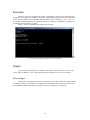
When the console application is called, a new window will appear on the screen. This window is
the console application and is an entity unto itself. It neither knows nor cares about the existence of the
Splash GUI. Similarly, the Splash GUI has no way of knowing what sort of progress the console
application has made. The upside of this behavior is that the GUI isn't completely locked up while itawaits
for simulation results from the number cruncher. The downside of this behavior is the user must use a
small bit of self control and adhere to the following:
1.
2.
3.
Do not attempt to run the console application again until the console application has
closed itself.
Do not attempt to access trajectory files (either from a DOS window or through the GUI)
until the console application indicates that it has started on its second iteration.
Do not attempt to access the splash pattern file (either from a DOS window or through
the GUI) until the console application has closed itself.
The GUI should prevent the user from doing any of the above, nonetheless the user is to
consider himself warned lest he find a way to circumvent the GUI's efforts at preventing the user from
doing something stupid.
The console application as it starts the 4th iteration out of 10 requested.
11
The data is saved exactly as if the user had selected "Save" from the "File" pull-down menu. This step is
required due to the program architecture employed by Splash.
24
Output
The Splash console application generates anywhere from four to six data streams depending upon
the number of stages to be modeled in the simulation. These streams provide user feedback, trajectory
data, and splash pattern data.
The most obvious of these streams is the text sent to the console application’s window. The
console application output (seen above) provides no data concerning scenario specifics but it does provide
the user with information regarding overall simulation progress. In other words, it displays a counter
showing how many iterations were requested and which iteration is currently being processed - nothing
less, nothing more.
The remaining data streams are all ASCII text files of fixed column width for easy import into
spreadsheets and other data processing applications. But while these text files are designed for easy import
into other applications, the Splash GUI does include it’s own (albeit limited) capability to quickly examine
these text files in a graphical environment. Each of these text files and the Splash GUI interface for
examining them is discussed below.
Splash Pattern Files/Window
As one may imagine, the splash pattern data file contains the impact locations (longitude and
latitude) for each stage for each Assuming a scenario base filename of “alpha,” the splash pattern data file
will be named “ spash_spl.out”. A crudely formatted graphical representation of this data may be viewed
by selection “Splash Pattern” from the “Output” pull-down menu at the top of the Splash GUI’s main
window.
Those who endeavor to import the data in the splash pattern file into other applications no doubt
harbor a desire to know the exact formatting of the splash pattern file. In tabular format, the columns found
with the splash pattern data file are as follows:
Column
Run
1Longitude
1Latitude
2Longitude
2Latitude
3Longitude
3Latitude
Description
The iteration or run number. While most runs include the randomization
required of a Monte-Carlo analysis, it should be noted that the 0th run does not
include any randomization. In other words, the 0th run is the nominal trajectory.
Longitude of the 1st stage impact point in degrees. A negative angle corresponds
to West longitude.
Latitude of the 1st stage impact point in degrees. A negative angle corresponds to
South latitude.
Longitude of the 2nd stage impact point in degrees. A negative angle corresponds
to West longitude.
Latitude of the 2nd stage impact point in degrees. A negative angle corresponds
to South latitude.
Longitude of the 3rd stage impact point in degrees. A negative angle corresponds
to West longitude.
Latitude of the 3rd stage impact point in degrees. A negative angle corresponds
to South latitude.
25
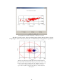
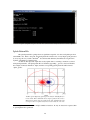
The Splash Pattern window displaying a 100 impact scenario.
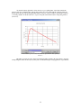
The author concedes, however, that for presentation quality graphics, the user is likely to be better
off importing the data from the trajectory file(s) into a dedicated data processing application or spreadsheet.
An Excel plot displaying splash pattern data for 1000 flights of a
boosted dart. Blue diamonds denote impact point for the booster. Red
triangles denote impact points for the dart. Similarly the blue oval
represents a 3-sigma oval for the booster while the red circle
represents a 3-sigma oval for the dart. The green dot denotes the
launch point.
26
Trajectory Data Files/Window
Splash generates anywhere from two to four trajectory files. These files contain the flight
parameters for the nominal mission12 outlined in the input windows. One file is produced for each stage (13) and an additional file is generated that tracks the "topmost" active stage (I.E., generates a single nominal
trajectory based on the trajectories of all activated stages.).
Each trajectory file tracks a total of 33 parameters. While more detailed discussion is found in the
sections of the manual dedicated to the console application, it may suffice to say that the data tracked is the
following (in tabular format):
Column
Time
Longitude
Latitude
Altitude
Azmth
Eleva
Roll
AbsVel
RelVel
AirVel
YawRt
PitRt
RolRt
Gamma
Headg
Mach
AOA
Axial
Ca
Normal
Cn
Mass
Mdot
Thrust1
Thrust2
Thrust3
Thrust4
Thrust5
Prop1
Prop2
Prop3
Prop4
Prop5
12
Description
Total time elapsed since beginning of simulation (s).
Longitude (deg).
Latitude (deg).
Altitude (m or ft, ASL).
Body azimuth (deg).
Body elevation (deg).
Body roll (deg).
Velocity with respect to the center of the Earth (m/s or ft/s).
Velocity with respect to a point on the surface of the Earth at the same longitude
and latitude as the vehicle (m/s or ft/s).
Velocity with respect to the local air, i.e., air speed (m/s or ft/s).
Yaw rate (deg/s).
Pitch rate (deg/s).
Roll rate (deg/s).
Flight angle (deg).
Heading (deg).
Mach number.
Angle of attack (deg).
Axial aerodynamic force (N or lbf).
Axial aerodynamic force coefficient normalized to the vehicle’s nominal frontal
area.
Normal aerodynamic force (N or lbf).
Normal aerodynamic force coefficient normalized to the vehicle’s nominal
frontal area.
Total vehicle mass (kg or lbm).
Combined mass flow rate (kg/s or lbm/s) through all 5 motor nozzles.
Thrust (N or lbf) generated by motor 1.
Thrust (N or lbf) generated by motor 2.
Thrust (N or lbf) generated by motor 3.
Thrust (N or lbf) generated by motor 4.
Thrust (N or lbf) generated by motor 5.
Propellant (kg or lbm) remaining in motor 1.
Propellant (kg or lbm) remaining in motor 2.
Propellant (kg or lbm) remaining in motor 3.
Propellant (kg or lbm) remaining in motor 4.
Propellant (kg or lbm) remaining in motor 5.
No failures, all mission parameters exactly as found in input files/windows.
27
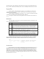
As stated elsewhere, Splash also allows the user to get a quick glimse of the data found in the
trajectory files in a graphical format. The plotting routines are accessed through the "Output" pull-down
menu found at the top of the main Splash GUI window. The use of these routines is trivial and is reduced
to selecting variables for the X and Y axis of a plot from pull-down menus found on the plotting window
(see below).
A time/altitude plot viewed from within the Splash GUI'sdata plotting
interface.
The author concedes, however, that for presentation quality graphics, the user is likely to be better
off importing the data from the trajectory file(s) into a dedicated data processing application or spreadsheet.
28
The Console Application
29
Description
The heart and soul of Splash is a console application that may be run independent of the GUI.
While the console application is not as easy to use without the GUI, it allows the user to directly
manipulate the simulation input files. In the author’s experience, such direct manipulation often allows the
user to simulate conditions not anticipated (and thus often not directly supported) by the original author.
As a result direct manipulation of the data files and use of the console application is considered to be the
modus operandi of the serious user. Thus, some discussion of this is in order.
Input Requirements
While many simulation packages include all data pertinent to a scenario in a single input file,
Splash separates the data into two to five data files (depending upon the number of stages in the rocket) of
2 different classifications. The two different types of data files are as follows: scenario files and stage files.
Each of these two file types will be discussed in detail, but first it is appropriate to outline some basic
conventions that hold true for all Splash input files.
General Input Conventions
First and foremost, data files used by Splash are simple text files. While not as compact or as
elegant as other file formats, text files allow for simple file manipulation and manual inspection for file
accuracy. Historically, many simulation packages that utilize text data files have relied upon a very strict
data formatting structure. While some rules must apply, every attempt has been made to make Splash input
files easy to read for mere humans. As a result, the following may be said:
•
Blank lines are ignored.
•
Data is white space and/or comma delimited. In other words, data items within a single line are
delimited by any number of commas, spaces, or tab spaces.
•
The occurrence of an asterisk (“*”) denotes that any remaining text on a given line are comments
and to be ignored by Splash
•
A single line of data is limited to 240 characters.
To better illustrate the conventions of data input, below are a number of examples of lines of data
that are 100% equivalent within the context of Splash input files.
27.3 62610.0
0.008 * <-- That asterisk indicates comments!
27.3, 62.61e3, 8e-3
* Propelant(kg), It(N*s), Nozzle (m^2)
27.3,,62610,
.008
* Propelant, It, Nozzle Exit Area
27.3 62610
8E-3
* Are we getting the picture?
Each data file’s name must also conform to a standard naming convention. Again, the details of
each file will be discussed later, but suffice to say that the names are all variations of a single file name
referred to as the “base file name ”.
In addition to the conventions listed above, scenario and stage data files employ the use of “data
blocks.” Data blocks are small clusters of data to break down the file into more intuitive, easier to use
chunks of data. For example, each stage data file contains a propulsion system data block. As one might
guess, the this data block contains all data pertaining to the rocket motors for that particular stage. While
data within each individual data block must be found in a particular order, it should be noted that the order
30
data blocks appear in a file is unimportant. This means that one may place often-modified data blocks at
the top of a file to facilitate faster modification due to the ease of finding the desired block in a text editor.
Scenario Files
Scenario data files contain all information required to set up a launch that is not related to the
rocket itself. In other words, scenario data files contain information on the launch rail, the weather, the
local terrain, and any uncertainties.
Scenario data files are identified by a file extension of “ .scn”. In other words, if the base file name
is “alpha”, the corresponding scenario data file must be named “ alpha.scn” .
A description of each data block (listed in alphabetical order) found in the scenario data file is as
follows:
Rail Data Block
As it’s name implies, the rail data block contains all information pertinent to the launch rail. The
format of the rail data block is as follows:
Line
1
2
3
4
5
Contents
Must contain the pneumonic “RAIL”.
Must contain 3 numeric arguments. In order, they are the launch rail’s longitude
(degrees), latitude (degrees), and altitude (meters, ASL). Note that West longitude is
denoted as a negative angle while South latitude is likewise considered a negative
angle.
Must contain 3 numeric arguments. In order they are the launch rail’s azimuth
(degrees), elevation (degrees), and length (meters). Note that the convention used
within Splash dictates that a negative elevation is pointing “up”.
Must contain 1 numeric argument. This argument is the initial velocity of the rocket in
meters per second. Most of the time this argument will be set to zero, but the user was
left with the option of non-zero initial velocities to crudely model a gun-launched
rocket or similar system that may have a non-negligible velocity at motor ignition.
Must contain the data block termination string, “-----“.
A sample rail data block may be seen below. This data indicates that a rocket is to be launched
due East and at an elevation angle of 80 degrees (10 degrees off vertical) from the author’s backyard in
Southern California. The launch rail is 10 meters long and the initial velocity is 0 meters per second.
RAIL
-117.6726 35.6337 728.2
90.0
-80.0
10.0
0
-----
* Longitude, Latitude, Altitude (ASL)
* azimuth, elevation, rail length
* velocity
Terrain Data Block
The terrain data block does nothing more than define the local terrain’s altitude above sea level in
the landing zone. For most cases, the local terrain and the launch rail will be at the same altitude, but
Splash allows the user to define separate altitudes for the launch and impact areas. The most obvious use
of this feature is to crudely simulate an air launch, but it may find use in terrestrial launches as well to
simulate other exotic systems. Note that a rocket has been deemed to impact the Earth when it’s altitude
falls below the terrain altitude and it’s flight angle (gamma) indicates the rocket is in a dive. The format of
the terrain data block is as follows:
31
Line
1
2
3
Contents
Must contain the pneumonic “TERRAIN”.
Must contain a single numeric argument. This argument defines the altitude of the
impact area in meters above sea level.
Must contain the data block termination string, “-----“.
Although they are very simple, a sample terrain data block is shown below for completeness.
TERRAIN
728
* Local terrain is about 2300 feet ASL
----Uncertainty Data Block
Uncertainty data blocks contain information on all parameters that are to be modified in the
generation of the splash pattern. The format of the splash data file is as follows:
Line
1
2
3
4
5
6
7
8
9
10
11
12
13
14
15
16
17
18
19
13
14
Contents
Must contain the pneumonic “UNCERTAINTY”.
Contains the total number of iterations desired. For mission planning, 1 is all you will
want, but for a full-blown splash pattern to be submitted to the FAA as part of a launch
license application 5,000 – 10,000 are probably better numbers.
Contains the launch mass 1-sigma uncertainty as a percentage of the total mass.
Contains the 1-sigma uncertainty of the moments of inertia as a percentage of the
moment of inertia for the axis in question.
Contains the 1-sigma uncertainty of the location of the center of gravity as a number of
calibers.
Contains the 1-sigma uncertainty in axial aerodynamic force coefficient (Ca) as a
percentage.
Contains the 1-sigma uncertainty in normal aerodynamic force coefficient (Cn) as a
percentage.
Contains the 1-sigma uncertainty of the location of the center of pressure as a number
of calibers.
Contains the 1-sigma uncertainty of the fin cant angle in degrees.
Contains the 1-sigma uncertainty of each rocket motor’s total impulse as a percentage
of the total impulse.
Contains the 1-sigma uncertainty of the propellant mass for each rocket motor as a
percentage of said mass.
Contains the 1-sigma uncertainty for each motor’s thrust alignment (i.e., thrust
misalignment) in degrees.
Contains the probability of an ignition failure for each motor as a percentage. 0
indicates a 100% reliable ignition, 100 indicates a 100% likelihood of ignition failure.
Contains the probability of a catastrophic failure (CATO) for each motor as a
percentage. Note that if any motor CATOs it is assumed that all other motors in the
same stage suffer a similar failure due to debris impact.
Contains the probability of a failure to deploy13 the recovery system as a percentage.
Contains the probability of a parachute/vehicle separation14 as a percentage.
Contains the 1-sigma uncertainty for wind velocity in meters per second.
Contains the 1-sigma uncertainty for wind direction in degrees.
Contains the 1-sigma uncertainty for launch rail azimuth in degrees.
Commonly referred to as a “lawn dart”.
Commonly referred to as a “zipper”.
32
20
21
Contains the 1-sigma uncertainty for launch rail elevation uncertainty in degrees.
Must contain the data termination string, “-----“.
A sample uncertainty data block is shown below.
UNCERTAINTY
1000
* How many times do we
*MASS
3
* Mass
2
* Moments of Inertia
0.25
* CG
*AERODYNAMIC
10
* Ca
10
* Cn
1
* CP
0.25
* Fin Cant Angle
*PROPULSION
5
* Total Impulse
1
* Propellant Mass
0.25
* Thrust Misalignment
*FAILURE
2
* Ignition
1
* CATO
5
* Deployment Failure
10
* Chute Failure
*WEATHER
3
* Wind Velocity
10
* Wind Direction
*RAIL
5
* Azimuth Error
1
* Elevation Error
-----
want to play?
(1 sigma uncertainty - percent)
(1 sigma uncertainty - percent)
(1 sigma uncertainty - calibers)
(1
(1
(1
(1
sigma
sigma
sigma
sigma
uncertainty
uncertainty
uncertainty
uncertainty
-
percent)
percent)
calibers)
degrees)
(1 sigma uncertainty - percent)
(1 sigma uncertainty - percent)
(1 sigma uncertainty - degrees)
(failure
(failure
(failure
(failure
likelihood
likelihood
likelihood
likelihood
-
percent)
percent)
percent)
percent)
(1 sigma uncertainty - mps)
(1 sigma uncertainty - degrees)
(1 sigma uncertainty - degrees)
(1 sigma uncertainty - degrees)
Weather Data Block
Again, the name of the data block is indicative of what data it contains. In this case, the data block
contains the local atmospheric conditions. Wind conditions obviously affect weather cocking, but local
barometric pressure and temperature effects density altitude which in turn effects lift, drag, and thrust
generated by the rocket. The format for the weather data block is as follows:
Line
1
2
3
4
Contents
Must contain the pneumonic “WEATHER”.
Must contain 2 numeric arguments. In order they are the launch site’s current
barometric pressure (mmHg) and temperature (oC). If the current barometric pressure
is unknown or if the user simply wishes to use a standard atmosphere, a negative value
for barometric pressure will turn off atmospheric corrections.
Must contain at least 2 and no more than 24 numeric arguments. These arguments are
a list of altitudes (m ASL) for which corresponding wind direction data (see line 4) is
valid.
Must contain the same number of numeric arguments as line 3. As previously
mentioned, these arguments define the direction (degrees) in which the wind is coming
from. 0 degrees indicates a wind from the North, 90 degrees represents a wind from
the East, and so on. Note that it is good practice to make the last 2 arguments identical
to avoid any unchecked extrapolation in the event the vehicle exits the defined weather
33
5
6
7
patterns.
Must contain at least 2 and no more than 24 numeric arguments. These arguments are
a list of altitudes (m ASL) for which corresponding wind velocity data (see line 6) is
valid. Note that in practice lines 3 and 5 will most likely be identical but there is
nothing in Splash programming logic that dictates this.
Must contain the same number of numeric arguments as line 5. As previously
mentioned, these arguments define the velocity (m/s) of the wind. As with line 4, it is
good practice to make the last 2 arguments identical to avoid any unchecked
extrapolation in the event the vehicle exits the defined weather patterns.
Must contain the data block termination string, “-----“.
A sample weather data block may be seen below.
WEATHER
* A hot day with low level winds from
* the N and high level winds from the NNE.
760 43.5
0 1e3 2e3 5e3 10e3 20e3 21e3
0
0
0 23.5 22.5 22.5 22.5
0 1e3 2e3 5e3 10e3 20e3 21e3
1
2
3
5
20
25
25
-----
Stage Files
Stage data files describe all parameters that are included within the vehicle itself. This includes all
aerodynamic and propulsion performance as well as information regarding staging and recovery. If a fullup rocket incorporates more than one stage, then a stage data file is required for each stage (The maximum
number of stages is 3.).
Stage data files are identified by a file extension of “ .stg”, but the naming of a stage data file is not
just a matter of appending “. stg” to the base file name as would be expected given the naming conventions
of the scenario and splash data files. Rather, the stage number and “ .stg” must be appended to the base file
name. In other words, if the base file name is “alpha”, the corresponding stage data file for a first stage
must be named “alpha1.stg”. Similarly, the stage data file for the second stage is “alpha2.stg” and the stage
data file for the third stage is “alpha3.stg”.
As with the scenario data file, a stage data file is further subdivided into data blocks. These data
blocks may appear in any order within the stage data file, but all must appear. The format of each of these
data blocks is discussed below (in alphabetical order).
Axial Force Data Block
As one may imagine, the axial force data block contains information on the thrust-off axial force.
Most simulation packages store a list of axial force coefficients (Ca’s) for direct use in axial force
calculations; Splash, on the other hand, uses lists of coefficients of a polynomial that is in turn used to
calculate an axial force coefficient. In other words, Splash calculates the axial force coefficient by using an
equation of the form…
34
Ca = A + B * AOA + C * AOA2
where :
Ca = axial force coefficient (degrees)
A, B, C = polynomial coefficients
AOA = angle of attack
Extreme care should be used when selecting the values for A, B, and C in the above equation as
poorly selected values will yield wildly inaccurate simulation results. More to the point, one should ensure
that the values selected for A, B, and C produce a Ca of 0.0 at an angle of attack of 90 degrees.
While this methodology provides a smooth curve for Ca over a broad range of angles of attack
with minimal user input, it neglects the fact that axial force coefficients depend on Mach number. For this
reason, Splash employs not one set of coefficients, but a family of coefficients.
The format for the axial force data block is as follows:
Line
1
2
3
4
5
6
7
Contents
Must contain the pneumonic “CA”.
Must contain the axial force “multiplier”. This is a number by which the final axial
force is multiplied. Usually the value of this number is 1.0, but any number can be
used in the course of sensitivity studies. For example, if the user wishes to increase
axial force by 10% in an attempt to see what would happen, he need only input 1.1 as
the multiplier rather than generate a new drag curve.
Must contain at least 2 but no more than 24 numeric arguments. These arguments are
the Mach numbers for which the axial force coefficients (see lines 4-6) are valid.
Must contain at least 2 but no more than 24 numeric arguments. These arguments are
the 0th order axial force coefficients corresponding to the Mach numbers listed in line
3.
Must contain at least 2 but no more than 24 numeric arguments. These arguments are
the 1st order axial force coefficients corresponding to the Mach numbers listed in line
3.
Must contain at least 2 but no more than 24 numeric arguments. These arguments are
the 2nd order axial force coefficients corresponding to the Mach numbers listed in
line 3.
Must contain the data block termination string, “-----“.
A sample axial force data block may be seen below, notice that the first row of coefficients (the
“A” row) are simply the zero lift axial force coefficients which are equivalent to zero lift drag coefficients.
CA * For each Mach: Ca(AOA) = A + B*AOA +
1.0
0.2
0.8
1.2
1.75
2.5
3.5
0.97 0.91
1.66
1.42
1.27
1.11
-0.035 0.015 -0.086 -0.022 -0.024 -0.010
0.0027 7e-4 0.0047 0.0014 0.0020 0.0011
-----
C*AOA^2
*
*
*
*
Mach
A
B
C
Base Drag Data Block
The base drag data block is nothing more than a one dimensional look up table of base drag
coefficients (the portion of a vehicle’s zero lift drag 15 that is due to drag at the base of the vehicle). This
data is used to calculate the difference in axial force between thrust on and off conditions.
15
At zero angle of attack, drag and axial force are identical.
35
Note that one should ensure that the actual base drag coefficient is used; some aeroprediction
codes produce a base pressure coefficient. A base pressure coefficient is not the same thing as a base drag
coefficient. If in doubt, entry of zeros is probably the best bet.
The format of the base drag data block is as follows:
Line
1
2
3
4
Contents
Must contain the pneumonic “CB”.
Must contain at least 2 but no more than 24 numeric arguments. These arguments are
the Mach numbers for which the base drag coefficients (see line 3) are valid for.
Must contain at least 2 but no more than 24 numeric arguments. These arguments are
the base drag coefficients corresponding to the Mach numbers listed in line 2.
Must contain the data block termination string, “-----“.
A sample base drag data block is shown below.
CB
0.2 0.8 0.9 1.0 1.2 1.4 1.75 2.5 3.5
0.15 0.15 0.16 0.22 0.23 0.20 0.17 0.12 0.08
-----
* Mach
* Cb
Center of Gravity Data Block
The center of gravity data block is nothing more than a one dimensional look up table listing the
center of gravity (in calibers) and corresponding masses representative of various instants during a rocket’s
burn.
The format of the center of gravity data block is as follows:
Line
1
2
3
4
Contents
Must contain the pneumonic “CG”.
Must contain at least 2 but no more than 24 numeric arguments. These arguments are
the masses (kg) numbers for which the centers of gravity (see line 3) are valid for.
Must contain at least 2 but no more than 24 numeric arguments. These arguments are
the centers of gravity corresponding to the masses listed in line 2.
Must contain the data block termination string, “-----“.
A sample center of gravity data block is shown below. While this data block indicates a simple
linear relationship between a launch mass and a burnout mass, there is no reason why a more complex
relationship could not be used.
CG
58.2
12.0
-----
85.5
11.4
* Mass
* CG/Dref
Center of Pressure Data Block
As one may imagine, the center of pressure data block contains information on the center of
aerodynamic pressure. Most simulation packages store a list of centers of pressure (CP’s) for direct use in
pitching moment calculations; Splash, on the other hand, uses lists of coefficients of a polynomial that is in
turn used to calculate a center of pressure. In other words, Splash calculates the center of pressure by using
an equation of the form…
36
CP = A + B * AOA + C * AOA 2
where :
CP = center of pressure (calibers)
A, B, C = polynomial coefficients
AOA = angle of attack
But while this equation provides a smooth center of pressure movement with a minimum of input
requirements, it neglects the fact that the center of pressure also depends on Mach number. For this reason,
Splash employs not one set of coefficients, but a family of coefficients.
The format for the axial force data block is as follows:
Line
1
2
3
4
5
6
7
Contents
Must contain the pneumonic “CP”.
Must contain a single numeric argument, the center of pressure (CP) offset. The CP
offset provides a simple way for the user to vary the CP as one may during the course
of a sensitivity study. While a nominal CP is calculated as described previously, the
CP offset is added to this value to move the CP fore or aft as desired. For example, if
the user wishes to move the CP back one caliber, the CP offset should be 1.0.
Similarly, if the user wishes to move the CP foreward 0.5 calibers, the CP offset
should be –0.5. Obviously, 0.0 is the value normally selected.
Must contain at least 2 but no more than 24 numeric arguments. These arguments are
the Mach numbers for which the center of pressure coefficients (see lines 3-5) are
valid.
Must contain at least 2 but no more than 24 numeric arguments. These arguments are
the 0th order normal force coefficients corresponding to the Mach numbers listed in
line 3.
Must contain at least 2 but no more than 24 numeric arguments. These arguments are
the 1st order normal force coefficients corresponding to the Mach numbers listed in
line 3.
Must contain at least 2 but no more than 24 numeric arguments. These arguments are
the 2nd order normal force coefficients corresponding to the Mach numbers listed in
line 3.
Must contain the data block termination string, “-----“.
A sample center of pressure data block may be seen below.
CP
* For each Mach: CP(AOA) = A + B*AOA + C*AOA^2
0.0
0.2
0.5
0.9
0.95
1.05
1.1
* Mach
14
14
14
13
13
13
* A
0.01 0.01 0.01
0.01
0.01
0.01
* B
0.0
0.0
0.0
0.0
0.0
0.0
* C
----Fin Data Block
While the overall aerodynamic properties of the vehicle are primarily contained within the other
data blocks, the fin data block, while obviously containing information on the vehicle’s fins, is concerned
with vehicle yaw/pitch damping and roll16 and does not effect simple axial or normal force calculations.
16
Splash uses some non-standard methodologies that appear to yield reasonable results while reducing the
degree of sophistication required of the user in producing input data.
37
Before line-by-line discussion of the format of the fin data block, it should be noted that several
lines of the fin data block are devoted to defining the normal force coefficient of a single fin. The method
in which these coefficients are calculated is identical to that used in the Axial Force Data Block to calculate
axial force coefficients. The fin normal force coefficients are not, however, used to calculate axial or
normal forces experienced by the vehicle; they are used strictly for calculations involving yaw/pitch
damping and roll moments. For this reason, it is not terribly important to have exact numbers and in fact,
the numbers listed in the sample file may be sufficiently accurate for most applications.
The format for the fin data block is as follows:
Line
1
2
3
4
5
6
7
8
9
10
Contents
Must contain the pneumonic “FINS”.
Must contain an integer defining the number of fins the rocket has. Note that while
program logic will allow for any number of fins, realistically the methods employed
in Splash dictate that no more than 6 fins be used.
Must contain a numeric argument defining the planer area of a single fin as multiple
of the cross sectional area of the vehicle. While obviously a non-standard
nomenclature, this method allows the scaling of vehicles up or down with a minimum
of hassle.
Must contain two numeric arguments. The first of these arguments is the
longitudinal location of the fin’s center of pressure measured as the number of
vehicle calibers from the vehicle’s nose. The second argument is the radial location
of the fin’s center of pressure, again measured in calibers.
Must contain a single argument, the fin cant angle measured in degrees.
Must contain at least 2 but no more than 24 numeric arguments. These arguments are
the Mach numbers for which the fin normal force coefficients (see lines 7-9) are
valid.
Must contain at least 2 but no more than 24 numeric arguments. These arguments are
the 0th order normal force coefficients corresponding to the Mach numbers listed in
line 6.
Must contain at least 2 but no more than 24 numeric arguments. These arguments are
the 1st order normal force coefficients corresponding to the Mach numbers listed in
line 6.
Must contain at least 2 but no more than 24 numeric arguments. These arguments are
the 2nd order normal force coefficients corresponding to the Mach numbers listed in
line 6.
Must contain the data termination string “-----“.
A sample fin data block may be seen below. This data block, with the exception of lines 2-4, may
very well represent sufficiently accurate data for all the rockets the user ever desires to model.
FINS
* Polynomial is for FIN Cns
4
* number of fins
6
* FinArea/Aref
22
1
* CPx, CPr (in calibers)
0.0
* cant angle
0.0
0.8
1.4
1.75
2.5
3.5
0
0
0
0
0
0
0.022
0.022
0.022
0.022
0.022
0.022
-1.2e-4 -1.2e-4 -1.2e-4 -1.2e-4 -1.2e-4 -1.2e-4
----General Information Data Block
38
*
*
*
*
Mach
A
B
C
The general information data block contains a mixture of basic mass and geometry information
and staging information.
While the mass and geometry data is largely self-explanatory, the staging information is complex
in nature and unique to Splash. As a result, there is a discussion of staging criterion and formatting in the
section entitled “Staging and Recovery Criterion Explained.”
The format of the general information data block is as follows:
Line
1
2
3
4
5
6
Contents
Must contain the pneumonic “GENERAL”.
Must contain three numeric arguments. In order these arguments are the rocket’s
launch mass (kg), length (m), and reference diameter (m).
Must contain the first line of the staging criterion. As stated previously, staging
criterion will be discussed in detail in a later section of this manual.
Must contain the second line of the staging criterion.
Must contain the third line of the staging criterion.
Must contain the data block termination string “-----“.
A sample general information data block is shown below.
GENERAL
85.5 22.8
T >
6
G >
0
A < 1000
-----
0.13
*
*
*
*
Mass, length, diameter(Dref)
Staging criterion line 1
Staging criterion line 2
Staging criterion line 3
Inertial Tensor Data Block
While the contents of the inertial tensor data block may be intuitively obvious to some, it may not
be so obvious to others. For those without a background in 6DOF systems, the inertial tensor is nothing
more than a matrix that contains all the moments and products of inertia17 for a physical object.
The vehicle-based coordinate system used by Splash for the inertial tensor (and everything else) is
as follows:
Axis
X
Y
Z
Plain English Equivalent
Forward
Port (left)
Up
The format of the inertial tensor is as follows:
Line
1
2
3
4
5
Contents
Must contain the pneumonic “INERTIA”.
Must contain the gross vehicle mass (kg) at which the moment and products of inertia
calculations (lines 3-6) were made. This need not be the launch or burnout mass of
the vehicle.
4
Must contain three numeric arguments. In order these arguments are Ixx (m ), Ixy
4
4
(m ), and Ixz (m ).
4
Must contain three numeric arguments. In order these arguments are Iyx (m ), Iyy
4
4
(m ), and Iyz (m ).
4
Must contain three numeric arguments. In order these arguments are Izx (m ), Izy
17
If the user is unfamiliar with these terms, the author recommends researching them on the internet as
proper treatment of these topics would take more space than the author is willing to dedicate in these pages.
39
4
6
4
(m ), and Izz (m ).
Must contain the data block termination string, “-----“.
A sample inertial tensor data block is shown below.
INERTIA
80
.2
0
0
62
0
0
-----
0
0
62
* Ixx, Ixy, Ixz
* Iyx, Iyy, Iyz
* Izx, Izy, Izz
Normal Force Data Block
As one may imagine, the normal force data block contains information about the aerodynamic
normal force. Most simulation packages store a list of normal force coefficients (Cn’s) for direct use in
normal force calculations; Splash, on the other hand, uses lists of coefficients of a polynomial that is in turn
used to calculate a normal force coefficient. In other words, Splash calculates the normal force coefficient
by using an equation of the form…
C n = A + B * AOA + C * AOA2
where :
C n = normal force coefficient (degrees)
A, B, C = polynomial coefficients
AOA = angle of attack
But while this equation provides a smooth normal force curve with a minimum of input
requirements, it neglects the fact that normal force coefficients depend on Mach number. For this reason,
Splash employs not one set of coefficients, but a family of coefficients.
The format for the axial force data block is as follows:
Line
1
2
3
4
5
6
7
Contents
Must contain the pneumonic “CN”.
Must contain the normal force “multiplier”. This is a number by which the final
normal force is multiplied. Usually the value of this number is 1.0, but any number
can be used in the course of sensitivity studies. For example, if the user wishes to
increase normal force by 10% in an attempt to see what would happen, he need only
input 1.1 as the multiplier rather than generate a new drag curve.
Must contain at least 2 but no more than 24 numeric arguments. These arguments are
the Mach numbers for which the normal force coefficients (see lines 4-6) are valid.
Must contain at least 2 but no more than 24 numeric arguments. These arguments are
the 0th order normal force coefficients corresponding to the Mach numbers listed in
line 3.
Must contain at least 2 but no more than 24 numeric arguments. These arguments are
the 1st order normal force coefficients corresponding to the Mach numbers listed in
line 3.
Must contain at least 2 but no more than 24 numeric arguments. These arguments are
the 2nd order normal force coefficients corresponding to the Mach numbers listed in
line 3.
Must contain the data block termination string, “-----“.
A sample normal force data block may be seen below.
40
CN * For each Mach: Cn(AOA) = A + B*AOA + C*AOA^2
1.0
* Cn fudge factor
0.0
0.8
1.4
1.75
2.5
3.5
* Mach
0
0
0
0
0
0
* A
0.51 0.40
0.32
0.36
0.28
0.28
* B
0.019 0.022 0.027 0.024 0.022
0.018
* C
----Propulsion System Data Block
Obviously, the propulsion system defines the rocket motors driving the vehicle’s flight. What is
not obvious, however, is the fact that each stage is assumed to possess five rocket motors. No more. No
less. The motors are arranged in a manner similar to the five F-1’s found on the Saturn V. Those who are
not up on their rocketry history may instead refer to the sketch of the motor arrangement found below.
As seen from the aft end, the layout of the
five rocket motors found in each stage.
But not every vehicle has five motors; how is such a configuration suited to simulate vehicles with
fewer than five motors? In two words: null motors. While all five motors exist in program logic, there is
nothing in said logic that mandates these motors to provide any thrust or even have any propellant in them.
Thus, “excess” motors do not actually affect the vehicle’s flight in any way shape or form.
The format of the propulsion system data block is as follows:
Line
1
2
3
4
5
6
Contents
Must contain the pneumonic “MOTORS”.
Contains a string of up to 240 non-white space characters. This string is used by the
GUI to identify the motor but the 6DOF program logic does not use the string as
anything other than a placeholder (Which means that this line can not be left blank!).
Contains a single numeric argument. This argument represents a delay (in seconds
after stage separation/activation) before the motor is ignited. Generally this value
will be set to zero, but users who employ air-started motors or significant delays
before motor ignition after stage separation will find this feature useful.
Contains a single numeric argument. This argument represents the off-centerline
distance (in calibers) of the motor’s thrust axis . For the #1 motor (see diagram of
motor configuration) this number should always be zero. Similarly, it should always
be non-zero for the remaining four motors.
Contains three numeric arguments. These arguments (in order) are the motor’s
2
propellant mass (kg), sea level total impulse (N*s), and nozzle exit area (m ).
Must contain at least 3 but no more than 24 numeric arguments. These arguments are
41
7
8
9-15
16-22
23-29
30-36
a list of times (s) measured from motor ignition that correspond to thrust values listed
in line 7. Note that the first argument should always be 0.
Must contain at least 3 but no more than 24 numeric arguments. These arguments are
a list of instantaneous thrust levels (N) that correspond to the times listed in line 6.
The first and last of the listed thrusts should always be 0.
Must contain the data block termination string “-----“.
Identical in format to lines 2-8, but concerning motor number 2.
Identical in format to lines 2-8, but concerning motor number 3.
Identical in format to lines 2-8, but concerning motor number 4.
Identical in format to lines 2-8, but concerning motor number 5.
It should at this time be noted that the thrust/time curve entered is scaled such that a simple
trapezoidal integration of the scaled thrust/time curve will precisely match the user-defined total impulse.
Below is a sample propulsion system data block. It represents a 2 motor cluster of N class motors.
Notice that motors 1, 4, and 5, while still in the data file provide no input to vehicle performance, as they
have no propellant, total impulse, or nozzle exit area.
MOTORS
Motors/Null.EDX
0.0
0.0
0.0 0.0 0.0
0.0 1.0 1.0
0
1
0
----Motors/Custom1.EDX
0.0
0.25
13.5 31610
4e-3
0.0 0.01 0.13 0.23
0 2343 2003 1870
----Motors/Custom1.EDX
0.0
0.25
13.5 31610
4e-3
0.0 0.01 0.13 0.23
0 2343 2003 1870
----Motors/Null.EDX
0.0
0.25
0.0 0.0 0.0
0.0 1.0 1.0
0
1
0
----Motors/Null.EDX
0.0
0.25
0.0 0.0 0.0
0.0 1.0 1.0
0
1
0
-----
*
*
*
*
*
*
Type
Ignition delay
Off-centerline distance
Propellant, It, Aexit
Time
Thrust
* Type
* Ignition delay
* Off-centerline distance
* Propellant, It, Aexit
1.12 2.24 4.16 4.96 6.14 * Time
1310 1354 1434 450
0 * Thrust
* Type
* Ignition delay
* Off-centerline distance
* Propellant, It, Aexit
1.12 2.24 4.16 4.96 6.14 * Time
1310 1354 1434 450
0 * Thrust
42
*
*
*
*
*
*
Type
Ignition delay
Off-centerline distance
Propellant, It, Aexit
Time
Thrust
*
*
*
*
*
*
Type
Ignition delay
Off-centerline distance
Propellant, It, Aexit
Time
Thrust
Recovery System Data Block
The recovery system data block does exactly what one would assume it does; it defines the
recovery system. More to the point, the recovery system data block contains information on the
deployment and subsonic drag characteristics of the recovery system. Notice that the words “recovery
system” are used and not “parachute.” This is because Splash does not spend a lot of time doing detailed
modeling of the recovery system. It would thus be somewhat misleading to state that Splash models a
parachute. Nonetheless, the vehicle slows to the appropriate descent rate and even swings from side to
side, much as a rocket under a parachute would. In other words, it does a good enough job for the task at
hand.
While some of the data contained in this data bock is virtually self-explanatory, the deployment
information is complex in nature and unique to Splash. As a result, there is a discussion of deployment
criterion and formatting in the section entitled “Staging and Recovery Criterion Explained.”
The format of the recovery system data block is as follows:
Line
1
2
3
4
5
6
Contents
Must contain the pneumonic “RECOVERY”.
Must contain two numeric arguments. In order these arguments are the recovery
system’s subsonic drag coefficient, and nominal diameter 18 (m).
Must contain the first line of the deployment criterion. As stated previously, staging
criterion will be discussed in detail in a later section of this manual.
Must contain the second line of the deployment criterion.
Must contain the third line of the deployment criterion.
Must contain the data block termination string “-----“.
Staging and Recovery Criterion Explained
Within the general information and recovery system data blocks, there exist six lines of data that
have until now been unexplained. As these lines are collectively referred to as the staging and deployment
criterion, it is obvious that these lines control exactly when and where a vehicle stages or deploys it’s
recovery system.
Exactly how these lines control staging (and deployment) is actually quite simple. The staging
criterion is a collection of three logical tests that must be satisfied in order. Each test is a relatively simple
numerical comparison between a given simulation parameter (altitude, time, etc.) and a user-specified
trigger value. When the first test is found to be true, Splash begins to examine the second test. When the
second test is found to be true, Splash begins to examine the third test. When the third test is found to be
true, Splash separates the upper stage or deploys the recovery system as appropriate19.
While some examples will be shown shortly, it would be logical to first list the simulation
parameters available to the user for staging/deployment. The simulation parameters currently supported by
Splash for use in staging/deployment are:
Parameter
A
a
E
Description
Altitude. Trigger value units are meters above sea level. This parameter is most
likely useful to those using barometer-based deployment devices or a 6DOF
inertial measurement unit (IMU).
Change in altitude. Trigger value units are meters.
Body elevation angle (sometimes referred to as “theta”). Trigger value units are
degrees. By convention, -90 degrees specifies a vehicle pointing “straight up”
18
Assume a single parachute of circular section.
Note that a booster stage is allowed to separate from the sustainer and deploy a recovery system. These
events are completely independent of each other.
19
43
e
G
g
I
M
m
N
P
p
Q
q
T
t
while a +90 degrees specifies a vehicle pointing “straight down”. When using
deployment devices such as horizon detectors, this is most likely the parameter
one should use.
Change in body elevation angle.
Flight angle (sometimes referred to as “gamma”). . Trigger value units are
degrees. By convention, -90 degrees specifies a velocity vector pointing
“straight up” while a +90 degrees specifies a velocity vector pointing “straight
down”. This parameter is most likely useful to those using barometer-based
deployment devices or a 6DOF inertial measurement unit (IMU).
Change in flight angle.
Immediate. This parameter does not actually track any simulation variables. The
test in question is immediately valued as true and the simulation moves on to the
next criterion test line. Note that the direction and trigger values are still required
as place holders, but do not actually have any effect on simulation behavior.
Mach number. Trigger value is unitless. This parameter should only be used if
the vehicle in question utilizes a barometric unit.
Change in Mach number.
Never. This parameter does not actually track any simulation variables. The test
in question is perpetually valued as false and the simulation never moves on to
the next criterion line (and thus never stages/deploys). Note that the direction
and trigger values are still required as place holders, but do not actually have any
effect on simulation behavior.
Atmospheric pressure. Trigger value units are Pascals. Obviously, this
parameter should only be used if the vehicle in question utilizes a barometric
unit.
Change in atmospheric pressure.
Dynamic pressure (often referred to as “Q”). Trigger value units are Pascals.
Obviously, this parameter should only be used if the vehicle in question utilizes a
pitot tube in conjunction with a barometric unit.
Change in dynamic pressure.
Time. Trigger value units are seconds. This parameter should be used when the
vehicle in question utilizes a clock or pyrotechnic delay for staging/deployment.
Change in time.
Examples of possible user-desired scenarios and the corresponding staging/deployment criterion
may be seen below.
Desired Profile
Fly for a total of 10 seconds.
Stage/deploy.
Fly until missile “noses over” past horizontal.
Wait for missile to descend below 1000 m ASL.
Stage/deploy.
Fly to apogee.
Wait three seconds.
Stage/deploy.
Criterion Lines
T > 10.0
I > 0.0
I > 0.0
E > 0.0
A < 1000
I > 0.0
G > 0.0
t > 3.0
I > 0.0
At this point the user may have noticed that in the above examples the third test of the
staging/deployment criterion is always “I > 0.0”. This has nothing to do with program logic. Rather, it is
representative of the fact that two tests will most likely provide all the functionality required for 99% of the
users out there. The third test was included to incorporate that last 1% of users who may have more
complex requirements for staging/deployment timing.
44
Execution
Execution of the console application is trivial. From Windows, the user need only double click
the Splash console application executable. At this time, Splash will prompt the user for the base filename
for the scenario required. The base filename should be entered sans any extensions (“ .scn”, “. stg”, etc.).
For example, if the input data files for a particular scenario are “ alpha.scn” and “alpha1.stg”, then the user
should enter the base filename of “alpha”.
That’s it. After base filename entry Splash will do its thing.
screen capture of Splash prompting for the base filename.
A
Output
Upon execution, Splash produces a number of data streams. The first and most obvious is the
screen output. In addition to screen output, Splash generates anywhere from two to five data files.
Screen Output
The Splash console application produces very limited screen output. In fact, this output is limited
to nothing more than a progress update. As Splash begins each simulation iteration it echoes the current
iteration number and the total iterations requested by the user. Nothing more. Nothing less.
45
A screen capture of Splash as it processes the 12th of 10 iterations designated by the scenario “alpha”.
Splash Pattern File
The splash pattern file is perhaps the most significant output file; it is what sets Splash apart from
other 6DOF codes. More to the point, the splash pattern file contains a list of every impact point generated
by every stage in every scenario simulated20. It is this data that ultimately determines the 3-sigma circle
required of the FAA for a launch license.
As with all other input and output files used by Splash, there is a naming convention associated
with splash pattern files. All splash pattern files are named by appending “_ spl.out” to the base filename.
For example, if the base filename is “alpha”, then the corresponding splash pattern file will be named
“ alpha_spl.dat”.
An Excel plot displaying splash pattern data for 1000 flights of a
boosted dart. Blue diamonds denote impact point for the booster.
Red triangles denote impact points for the dart. Similarly the blue
oval represents a 3-sigma oval for the booster while the red circle
20
Assuming the scenario file calls for multiple simulation iterations. If only one iteration is requested, then
no splash pattern file is generated.
46
represents a 3-sigma oval for the dart. The green dot denotes the
launch point.
Splash pattern files are simple text files containing simple columns of data. The format of these
columns is as follows:
Column
Run
1Longitude
1Latitude
2Longitude
2Latitude
3Longitude
3Latitude
Description
The iteration or run number. While most runs include the randomization
required of a Monte-Carlo analysis, it should be noted that the 0th run does not
include any randomization. In other words, the 0th run is the nominal trajectory.
Longitude of the 1st stage impact point in degrees. A negative angle corresponds
to West longitude.
Latitude of the 1st stage impact point in degrees. A negative angle corresponds to
South latitude.
Longitude of the 2nd stage impact point in degrees. A negative angle corresponds
to West longitude.
Latitude of the 2nd stage impact point in degrees. A negative angle corresponds
to South latitude.
Longitude of the 3rd stage impact point in degrees. A negative angle corresponds
to West longitude.
Latitude of the 3rd stage impact point in degrees. A negative angle corresponds
to South latitude.
Trajectory Files
Splash generates anywhere from two to four trajectory files per execution. One file is generated to
describe each stage’s flight 21 and a final file compiles selected portions of the stage trajectory files to
generate a single nominal trajectory.
An Excel plot generated with time/altitude data taken from two
different Splash stage trajectory files illustrates the trajectory of
each stage of a boosted dart.
The most informative of Splash trajectory files are the stage trajectory files. These files contain
data concerning the flight of each individual stage from the moment it separates from the previous stage to
the moment it impacts the Earth.
21
Thus generating one, two, or three of these trajectories files as appropriate to the number of stages in the
vehicle.
47
Stage trajectory files share a common naming convention. Specifically, “ X.out” is appended to
the base filename where X is the number of the stage in question. For example, if the base filename of the
simulated scenario is “alpha”, then the trajectory data for the first stage would be found in the file named
“alpha1.out”. Similarly, the trajectory data for the second and third stages would be found in the files
“alpha2.out” and “alpha3.out” respectively.
The remaining trajectory file, the nominal trajectory file is the file that is most likely to be of
initial interest to users. This trajectory file combines the most “interesting” data from the stage trajectory
files to create a single trajectory. This trajectory describes the flight experienced by the vehicle if one
assumes that boosters are no longer of interest after they separate from later stages.
The name of the nominal trajectory file is nothing more than “ .out” appended to the scenario base
filename. For example, if the base filename of the simulated scenario is “alpha”, then the nominal
trajectory file is named “ alpha.out”.
Beyond the fact that the various trajectory files describe trajectories associated with different
objects, they are otherwise identical. All are text files. All share the same collimated data structure. The
format of the data found in these files is as follows:
Column
Time
Longitude
Latitude
Altitude
Azmth
Eleva
Roll
AbsVel
RelVel
AirVel
YawRt
PitRt
RolRt
Gamma
Headg
Mach
AOA
Axial
Ca
Normal
Cn
Mass
Mdot
Thrust1
Thrust2
Thrust3
Thrust4
Thrust5
Prop1
Prop2
Prop3
Prop4
Prop5
Description
Total time elapsed since beginning of simulation.
Longitude (deg).
Latitude (deg).
Altitude (m, ASL).
Body azimuth (deg).
Body elevation (deg).
Body roll (deg).
Velocity with respect to the center of the Earth (m/s).
Velocity with respect to a point on the surface of the Earth at the same longitude
and latitude as the vehicle (m/s).
Velocity with respect to the local air, i.e., air speed (m/s).
Yaw rate (deg/s).
Pitch rate (deg/s).
Roll rate (deg/s).
Flight angle (deg).
Heading (deg).
Mach number.
Angle of attack (deg).
Axial aerodynamic force (N).
Axial aerodynamic force coefficient normalized to the vehicle’s nominal frontal
area.
Normal aerodynamic force (N).
Normal aerodynamic force coefficient normalized to the vehicle’s nominal
frontal area.
Total vehicle mass (kg).
Combined mass flow rate (kg/s) through all 5 motor nozzles.
Thrust (N) generated by motor 1.
Thrust (N) generated by motor 2.
Thrust (N) generated by motor 3.
Thrust (N) generated by motor 4.
Thrust (N) generated by motor 5.
Propellant (kg) remaining in motor 1.
Propellant (kg) remaining in motor 2.
Propellant (kg) remaining in motor 3.
Propellant (kg) remaining in motor 4.
Propellant (kg) remaining in motor 5.
48
Appendices
49
Tips and Tricks
This portion of the manual is nothing more than a listing of tricks a user may employ to model
vehicles or situations that may not be obviously supported by Splash.
Dual Deployment
Many high altitude vehicles employ a 2-stage recovery system. That is to say that they deploy a
very small drogue chute at high altitude followed by the deployment of a large parachute at low altitude.
While Splash does not directly support such systems, it can be tricked into modeling such systems provided
that they are 2-stage or less vehicles. How?
1.
2.
3.
4.
Set up the input data files/windows normally.
Set the final stage's recovery criterion such that the deployment occurs at the same moment that it
is wished for the drogue chute on the dual deployment system to deploy. The recovery system
properties for this stage should match those of the drogue chute.
Set the final stage's staging criterion such that the stage separates at the same moment it is desired
for the main chute on the dual deployment system to deploy.
Create a new "final stage". This stage does not exist in reality; it only exists in the model. This
new stage should match the real final stage in every way shape and form, but it should deploy it's
recovery system immediately. The recovery system properties for this stage should match those of
the main parachute.
The result of such a scenario will match that of a vehicle equipped with a dual deployment system.
The only caveat is that some cutting and pasting will be in order to piece together the true trajectory from
the trajectory data files.
Vacuum Total Impulse
Some users who attempt to program a pre-existing motor into Splash may find a small bit of
confusion in the entry of total impulse. The performance parameters of many motors are listed under
vacuum conditions. Splash requires parameters to be under sea level conditions. In the event one is
unaware, a total impulse conversion between these two conditions is rather trivial.
SeaLevelImpulse = VacuumImpulse - NozzleExitArea * 101.3 kPa * BurnTime
…or if you prefer English units…
SeaLevelImpulse = VacuumImpulse - NozzleExitArea * 14.7 psi * BurnTime
50
Known Bugs
Excessive pitch oscillation during ballistic descent
Currently the only known bug in Splash concerns yaw/pitch damping during ballistic descent after
the vehicle experiences extremely high angles of attack (approx. > 160 degrees). Rooted within the
yaw/pitch damping algorithms, the bug results in a grossly underdamped yaw/pitch oscillation. This
oscillation will eventually dampen out rather quickly once the amplitude of the oscillation falls to about
280 degrees. In addition, it does not appear that vehicles under parachute suffer from the bug. Fortunately,
the extreme angles of attack that bring about this bug are rarely seen in realistic scenarios.
51
New Features & Bug Fixes
Version 1.1.0
1.
2.
3.
4.
5.
Support for English units was added to the GUI. Note that internally Splash still uses the SI
system.
The propulsion input window in the GUI was totally revamped. The new window is less
intimidating but just as easy to use.
A maximum flight time of 3600 seconds (1 hour) was inserted into the console application. This
allows users to "go for orbit" without putting Splash into an infinite loop.
As the copy protection scheme was giving a few users problems that ranged from cosmetic or
disastrous, this has been removed.
At users' request, the install routine now adds a shortcut to the Splash GUI to the desktop.
Version 1.0.1
1.
2.
The install routine now copies the User's Manual to the hard drive.
A small bug that could result in negative thrust under certain circumstances was fixed.
52
Software License
Hall Consulting Software License
This is a legal agreement between you, the end user, and Hall Consulting (HC). By installing and/or using
this software package you are agreeing to be bound by the terms of this agreement.
1) Grant of license. HC grants you the right to use one copy of the enclosed HC software program (the
"software") on a single computer. The software is in use on a computer when it is loaded into
temporary memory or installed into permanent memory of that computer.
2) Copyright. The software is owned by HC and is protected by the United States copyright laws and
international treaty provisions and all other applicable national laws. Therefore, you must treat the
software like any other copyrighted material except for the fact that installation on a computer
necessitates the creation of a copy of the software. You may not copy any written material that
accompanies the software.
3) Other Restrictions. You may not rent or lease the software, but you may transfer the software and
accompanying written materials on a permanent basis provided you retain no copies and the recipient
agrees to the terms of this agreement. If the software is an update or has been updated, any transfer
must include the most recent update and all previous versions. You may not reverse engineer,
decompile, or dissassemble the software.
4) U.S. Government Restricted Rights. The software and documentation are provided with restricted
rights. Use, duplication, or disclosure by the government is subject to restrictions as set forth in
subparagraph (c)(1)(ii) of The Rights in Technical Data and Computer Software caluse at DFARS
252.227-7013 or subparagraph (c)(1) and (2) of the Commercial Computer Software -- Restricted
Rights at 48 CFR 52.227-19, as applicable. Manufacturer is Hall Consulting, 320 W. Felspar Ave.,
Ridgecrest, CA 93555.
5) Warranty. Splash includes no warranty in any way shape or form. The user understands that while
Splash represents the very best efforts of HC, HC does not possess the resources to fully verify and
debug software in a manner consistent with major corporations.
53
About the Author
At this point, there are those who would rightfully question the capabilities of your average Joe to
write such software. With this question in mind, a brief resume of sorts is offered….
1993-1995
University Computing Services
University of Oklahoma
Provided technical support to students and faculty with an emphasis on
debugging programs written in ANSI compliant C.
1994
Awarded Bachelors of Science in Mechanical Engineering
University of Oklahoma
1995-2001
Weapons Engineering and Analysis Branch
Naval Air Warfare Center, Weapons Division
Authored and employed various 3 and 6 DOF codes to simulate
military weapon systems ranging from shoulder-fired rockets to IRBMs
for both design and range safety purposes.
2001-2002
Ordnance Test Support Branch
Naval Air Warfare Center, Weapons Division
Provide engineering support for ordnance testing activities. These
activities include the static firing of solid rocket motors of up to 1.5
million pounds thrust.
While this hardly qualifies the author as the world’s leading expert on rockets and 6 DOF codes, it
is hoped that the reader will concur that he’s been around the block enough times to do an adequate job.
The author aboard a gen-u-ine made
in theUSSR SA-2 Guide Line.
54
Glossary
3-sigma circle
Axial force
Azimuth
Base drag
Ca
CATO
Cb
Center of gravity
Center of pressure
Cn
Drag
Dynamic pressure
Elevation
Ignition failure
Lift
Moment of inertia
Normal force
Pitch
Product of inertia
Q
Roll
Specific impulse
Splash pattern
Total impulse
WGS-84
Yaw
Zipper
An imaginary circle (or oval) on the ground that encircles all potential impact
points of a given vehicle to three standard deviations.
The aerodynamic force acting along the longitudinal axis of a flight vehicle. At
zero degrees angle of attack, axial force is equivalent to drag.
An arc of the horizon measured between a fixed point and the vertical circle
passing through the center of an object. In astronomy and navigation azimuth is
usually measured clockwise from the north point through 360 degrees of
rotation.
The component of a vehicle's total drag that is due to aerodynamic effects at the
aft end of the vehicle.
The axial force coefficient
The catastrophic failure of a rocket motor usually characterized by the failure of
the motor casing.
The base drag coefficient
The location on a finite body through which the centroid of gravitational forces
acting on that body passes.
The location on a finite body through which the centroid of aerodynamic forces
acting on that body passes.
The normal force coefficient
The component of the total aerodynamic force acting on an airplane or airfoil
that acts opposite to the velocity vector of a vehicle.
The pressure exerted on a vehicle’s leading edges due to the pressure exerted by
moving air. Usually denoted as “Q”.
The angle of a vehicle or launch rail’s longitudinal axis with respect to
horizontal. Often denoted as “theta”.
A propulsion system failure defined by an igniter’s failure to ignite a motor’s
propellant grain in a manner consistent with sustained combustion of said grain.
The component of the total aerodynamic force acting on an airplane or airfoil
that acts perpendicular to the velocity vector.
A mass property that measures how "resistant" an object is to torque. More
precise definitions are somewhat complex and math intensive; the reader is
recommended to search for such a definition online.
The aerodynamic force acting perpendicular to the longitudinal axis of a flight
vehicle. At zero degrees angle of attack, normal force is equivalent to lift.
The portion of any angular offset of the vehicle’s longitudinal (X) axis with
respect to the velocity vector that is about the horizontal (Y) axis.
Closely related to the moment of inertia, the product of inertia measures the
dynamic balance of a rotating object. Again, precise definitions are complex
and math intensive; again an online search is recommended for clarification.
Dynamic pressure.
The angular position of a vehicle's dorsal fin or "top" with respect to horizontal.
Defined as the instantaneous thrust divided by propellant burn rate, specific
impulse proves a benchmark by which the efficiency of a propulsion system
may be measured.
A graphical representation illustrating numerous impact points of a given
vehicle on which a Monte Carlo uncertainty analysis has been performed.
Defined as the integral of a motor’s thrust/time curve, the total impulse provides
a benchmark by which the “size” of a motor may be measured.
The Earth model used in the Global Positioning System (GPS).
The portion of any angular offset of the vehicle’s longitudinal (X) axis with
respect to the velocity vector that is about the vertical (Z) axis.
A recovery system failure mode in which the parachute (or other drag-inducing
device) is physically separated from the rest of the vehicle.
55
Index
dual deployment ...............................................50
dynamic pressure ........................................44, 55
2
2-stage deployment...........................................50
E
3
Earth ...................................................................7
elevation .............................14, 15, 27, 31, 48, 55
execution.....................................................24, 45
3-sigma circle .............................................46, 55
A
F
aerodynamics................................................8, 16
air launch ..........................................................31
air speed......................................................27, 48
air start..............................................................41
altitude............................................14, 27, 43, 48
angle of attack ............................................27, 48
atmosphere....................................................7, 13
atmospheric pressure ........................................44
axial force.................................27, 32, 34, 48, 55
axial force coeficient ........................................16
axial force multiplier ........................................16
azimuth ...............................14, 15, 27, 31, 48, 55
failure................................................................15
fin area..............................................................18
fin cant ..................................................15, 18, 32
fins ..............................................................17, 37
flight angle..................................................27, 48
G
gamma ........................................................27, 48
geometry .....................................................18, 19
gravity.................................................................7
gun-launched ....................................................31
B
H
barometric pressure ....................................13, 33
base drag...............................................16, 35, 55
base file name.............................................12, 30
base pressure.....................................................36
body elevation angle.........................................43
bugs ..................................................................51
heading .......................................................27, 48
horizon detector ................................................43
I
ignition delay ..............................................21, 41
ignition failure ......................................15, 32, 55
impact ...............................................................31
impact area........................................................32
impact pattern ...................................................46
impact zone.......................................................14
inertial tensor ..............................................19, 39
initial velocity...................................................31
input conventions..............................................30
input requirements ..................................6, 12, 30
installation ........................................................10
iteration.....................................15, 25, 32, 45, 47
C
Ca .......................................15, 16, 27, 32, 48, 55
case failure........................................................15
cato ...................................................................15
CATO .........................................................32, 55
Cb ...............................................................16, 55
center of gravity....................7, 15, 19, 32, 36, 55
center of pressure............................15, 32, 36, 55
center of pressure offset....................................17
clustered motors ...............................................20
Cn .......................................15, 17, 27, 32, 48, 55
console application ...........................................29
coordinate system .............................................39
CP ...................................... See center of pressure
L
latitude ................................13, 25, 27, 31, 47, 48
launch mass ......................................................19
launch rail .................................14, 15, 31, 32, 33
launch site.........................................................12
lawn dart .....................................................15, 32
length ............................................................7, 19
lift .....................................................................55
location .............................................................13
longitude .............................13, 25, 27, 31, 47, 48
D
damping............................................................17
data blocks........................................................30
density altitude .................................................33
deployment .................................................15, 43
deployment failure............................................32
diameter ........................................................7, 19
drag...................................................................55
M
Mach.....................................................16, 27, 48
56
Mach number....................................................44
mass......................................7, 19, 27, 32, 39, 48
mass properties ...........................................15, 18
mdot............................................................27, 48
models ................................................................7
moment of inertia .............................7, 32, 39, 55
moments of inertia......................................15, 19
motor ................................................................41
failure probability .........................................32
motor clusters ...................................................20
motor failure .....................................................15
motor location...................................................21
motors...............................................................21
S
N
temperature .......................................................33
ambient .........................................................13
terrain..........................................................14, 31
theta ......................................................27, 43, 48
thrust...........................................................27, 48
thrust alignment ................................................15
thrust axis..........................................................41
thrust misalignment ..........................................32
thrust/time curve .........................................22, 41
time.......................................................27, 44, 48
total impulse .............................15, 21, 32, 41, 55
trajectory...........................................................47
trajectory file ....................................................27
scenario file ......................................................31
screen output.....................................................45
software license ................................................53
specific impulse ................................................55
splash pattern ........................................32, 46, 55
splash pattern file..............................................25
stage file............................................................34
staging ........................................................22, 39
staging criterion ................................................43
system requirements .........................................10
T
nominal diameter ..............................................19
nominal length..................................................19
normal force .............................27, 32, 40, 48, 55
normal force multiplier.....................................17
nozzle .........................................................21, 41
null motors........................................................20
O
output..........................................................25, 45
P
parachute ....................................................15, 22
parachute failure ...............................................32
pitch......................................................27, 48, 55
product of inertia ....................................7, 39, 55
products of inertia.............................................19
propellant..............................................27, 41, 48
propellant mass.....................................15, 21, 32
propulsion...............................................8, 15, 41
propulsion system.............................................19
U
uncertainties................................................14, 32
uninstall ............................................................10
unit system........................................................12
V
velocity .......................................................27, 48
W
Q
weather .............................................................33
weather cocking................................................33
WGS-84..................................................7, 13, 55
wind ................................................13, 15, 32, 33
Q 44, 55
R
rail ....................................................................14
recovery............................................................22
recovery criterion .............................................43
recovery system................................................43
recovery system failure.....................................15
reference area ...................................................18
roll ........................................................27, 48, 55
Y
yaw .......................................................27, 48, 55
Z
zipper ..........................................................32, 55
57