Download The Model-based Integrated Simulation Framework User`s Manual

The Model-based Integrated Simulation Framework
User’s Manual
MILAN v.1.1 release (March 2004)
Copyright © 2003, 2004 Institute for Software Integrated Systems,
Vanderbilt University, and the University of Southern California
Contact information:
For questions, comments, and suggestions, please signup for the milan-users mailing list at
http://list.isis.vanderbilt.edu/. For bug reporting related to MILAN or GME, please utilize the
ISIS bugzilla installation at http://bugzilla.isis.vanderbilt.edu.
Your comments and questions will be monitored and addressed by the MILAN development
team.
Project and tool information:
The MILAN toolset was developed through research supported by the Defense Advanced
Research Projects Agency (DARPA) under the Power Aware Computing and
Communication Program, contract F33615-C-00-1633. It is a joint development between
the University of Southern California and the Institute for Software Integrated Systems at
Vanderbilt University.
Useful links:
http://www.isis.vanderbilt.edu/projects/MILAN
http://milan.usc.edu
http://www.usc.edu
http://www.isis.vanderbilt.edu
http://list.isis.vanderbilt.edu
http://bugzilla.isis.vanderbilt.edu
Source Code available from:
machine: milan.isis.vanderbilt.edu
repository: /var/lib/milan
username: anonymous
Table of Contents
MILAN: A MODEL BASED INTEGRATED SIMULATION FRAMEWORK............................................................................................................... 1
MODEL INTEGRATED COMPUTING .......................................................................................................................................................................................... 1
MILAN OVERVIEW ................................................................................................................................................................................................................. 2
APPLICATION MODELING ................................................................................................................................................................................................. 4
DATAFLOW .............................................................................................................................................................................................................................. 4
Multi-granular Simulation Support .................................................................................................................................................................................... 5
Isolated Simulation Support................................................................................................................................................................................................ 5
Interfacing ........................................................................................................................................................................................................................... 5
SYNCHRONOUS AND ASYNCHRONOUS DATAFLOW ................................................................................................................................................................ 6
DATA TYPES ............................................................................................................................................................................................................................. 8
PARAMETERS ........................................................................................................................................................................................................................... 9
MULTIPLE-ASPECT MODELING .............................................................................................................................................................................................. 10
HARDWARE APPLICATION MODELING .................................................................................................................................................................................. 10
Hierarchical Modeling...................................................................................................................................................................................................... 12
Clocks ................................................................................................................................................................................................................................ 13
Multiple Aspects ................................................................................................................................................................................................................ 14
COMPOSING THE HARDWARE AND DATAFLOW PARADIGMS ................................................................................................................................................. 14
RESOURCE MODELING..................................................................................................................................................................................................... 15
RESOURCE METAMODEL ....................................................................................................................................................................................................... 16
Structural Modeling of Resources .................................................................................................................................................................................... 17
Resource Model Parameters............................................................................................................................................................................................. 18
Modeling of Operating States ........................................................................................................................................................................................... 19
Resource Modeling and Mapping..................................................................................................................................................................................... 21
DRIVING SIMULATORS FROM RESOURCE MODEL ................................................................................................................................................................. 21
RESOURCE MAPPING ........................................................................................................................................................................................................ 24
DESIGN SPACE EXPLORATION ...................................................................................................................................................................................... 26
DESIGN SPACE MODELING ..................................................................................................................................................................................................... 26
CONSTRAINT REPRESENTATION ............................................................................................................................................................................................ 26
DESIGN SPACE EXPLORATION AND PRUNING ........................................................................................................................................................................ 27
SIMULATION WITH MILAN ............................................................................................................................................................................................. 28
SIMULATORS .......................................................................................................................................................................................................................... 28
Simulators Integrated in MILAN ...................................................................................................................................................................................... 28
MODEL INTERPRETATION ...................................................................................................................................................................................................... 29
MATLAB............................................................................................................................................................................................................................ 30
SimpleScalar...................................................................................................................................................................................................................... 30
PowerAnalyzer .................................................................................................................................................................................................................. 30
SimplePower...................................................................................................................................................................................................................... 31
JouleTrack ......................................................................................................................................................................................................................... 31
ARMulator ......................................................................................................................................................................................................................... 31
CodeComposer Studio....................................................................................................................................................................................................... 31
SystemC ............................................................................................................................................................................................................................. 31
ActiveHDL ......................................................................................................................................................................................................................... 32
HiPerE............................................................................................................................................................................................................................... 32
EMSIM............................................................................................................................................................................................................................... 32
FEEDBACK OF SIMULATION RESULTS .................................................................................................................................................................................... 32
HIGH-LEVEL PERFORMANCE ESTIMATOR............................................................................................................................................................... 33
COMPONENT SPECIFIC PERFORMANCE ESTIMATION ............................................................................................................................................................ 34
SYSTEM-LEVEL PERFORMANCE ESTIMATION ....................................................................................................................................................................... 35
ACTIVITY REPORT ................................................................................................................................................................................................................. 36
GENERATING INPUT FOR HIPERE .......................................................................................................................................................................................... 37
USING HIPERE....................................................................................................................................................................................................................... 37
PERFORMANCE ESTIMATION BASED ON DUTY-CYCLE ......................................................................................................................................................... 38
DESIGN BROWSER FOR HIPERE ............................................................................................................................................................................................ 39
EXTENSIBILITY TOOLKIT (XTK)................................................................................................................................................................................... 42
FEEDBACK INTERPRETER GENERATION ................................................................................................................................................................................ 42
Operands ........................................................................................................................................................................................................................... 42
Operators........................................................................................................................................................................................................................... 43
Results ............................................................................................................................................................................................................................... 44
Examples ........................................................................................................................................................................................................................... 44
Usage................................................................................................................................................................................................................................. 45
Feedback Interpreter Usage ............................................................................................................................................................................................. 45
THE GRAPH LIBRARY ............................................................................................................................................................................................................ 45
Class Structure and Interface ........................................................................................................................................................................................... 45
Files ................................................................................................................................................................................................................................... 49
OPTIMAL MAPPING OF TASKS ONTO ADAPTIVE COMPUTING SYSTEMS ..................................................................................................... 50
GENERAL DEFINITION OF THE OPTIMIZATION PROBLEM ..................................................................................................................................................... 50
SOLVING SINGLE-METRIC OPTIMIZATION PROBLEMS............................................................................................................................................................ 52
Target hardware platforms ............................................................................................................................................................................................... 53
MAPPING OF A LINEAR ARRAY OF TASKS ONTO A SINGLE DEVICE ........................................................................................................................................ 53
MAPPING OF A LINEAR ARRAY OF TASKS ONTO MULTIPLE DEVICES .................................................................................................................................... 54
MODELING OF THE APPLICATION, RESOURCE, AND MAPPING ............................................................................................................................................. 54
SOLVING MULTI-METRIC OPTIMIZATION PROBLEMS ........................................................................................................................................................... 57
MODELING AND PERFORMANCE ESTIMATION OF FPGAS.................................................................................................................................. 60
CHALLENGES IN FPGA MODELING AND PERFORMANCE ANALYSIS.................................................................................................................................... 60
DOMAIN SPECIFIC MODELING ............................................................................................................................................................................................... 60
MODELING OF FPGA IN MILAN .......................................................................................................................................................................................... 61
PERFORMANCE ESTIMATION ................................................................................................................................................................................................. 65
FPGA BASED DESIGN AND APPLICATION DESIGN ................................................................................................................................................................ 65
MODELING AND DSE BASED ON MEMORY CONFIGURATIONS ......................................................................................................................... 67
MODELING MEMORY CONFIGURATIONS............................................................................................................................................................................... 67
ENHANCEMENTS TO HIPERE ................................................................................................................................................................................................. 69
PERFORMING DSE ................................................................................................................................................................................................................. 70
REFERENCES ........................................................................................................................................................................................................................ 72
1
Chapter
MILAN: A Model Based Integrated Simulation
Framework
The Model-based Integrated Simulation Framework (MILAN) is a model-based,
extensible simulation integration framework that facilitates rapid evaluation of different
performance metrics, such as power, latency, and throughput, at multiple levels of
granularity of a large class of embedded systems by seamlessly integrating different
widely-used simulators into a unified environment. MILAN is a joint effort by the
University of Southern California and Vanderbilt University and is supported by the
DARPA Power Aware Computing and Communication Program through contract
number F33615-C-00-1633 monitored by Wright Patterson Air Force Base.
This document will detail the different modeling concepts supported by MILAN, the
various simulators currently supported, and how to use MILAN. The reader is advised
to also examine the tutorials provided, as they provide step-by-step examples of using
MILAN. Additionally, documentation on the tools released with MILAN (e.g. Desert
and HiPerE) is included and should be referenced if either of these tools will be
employed.
Model Integrated Computing
MILAN is implemented using Model Integrated Computing ( please see [ 1 ],[ 2 ], and
[ 3 ] for more information). MIC employs domain-specific models to represent the
system being designed. These models are then used to automatically synthesize other
artifacts. This approach speeds up the design cycle, facilitates the evolution of the
application, and helps system maintenance, dramatically reducing costs during the
entire lifecycle of the system. MIC is implemented by the Generic Modeling
Environment (GME), a metaprogrammable toolkit for creating domain-specific
modeling environments. GME employs metamodels that specify the modeling
paradigm of the application domain. The modeling paradigm contains all the syntactic,
semantic, and presentation information regarding the domain – which concepts will be
used to construct models, what relationships may exist among those concepts, how the
concepts may be organized and viewed by the modeler, and rules governing the
construction of models. The modeling paradigm defines the family of models that can
be created using the resultant modeling environment. The metamodels specifying the
modeling paradigm are used to automatically configure GME for the domain.
1
GME is used primarily for model-building. The models take the form of graphical,
multi-aspect, attributed entity-relationship diagrams. The static semantics of a model
are specified by OCL constraints [ 4 ] that are part of the metamodels. They are
enforced by a built-in constraint manager during model building time. The dynamic
semantics are applied by the model interpreters, i.e. by the process of translating the
models to source code, configuration files, database schema or any other artifact the
given application domain calls for.
MILAN overview
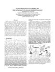
The MILAN architecture is depicted in Figure 1. The design-space of a system is
captured by multiple-aspect, hierarchical, primarily graphical models in GME. The
three main categories of models specify the desired application functionality, available
hardware resources and non-functional requirements in the form of explicit
constraints. These complex models typically specify an exponentially large designspace. However, only a subset of this space satisfies all the constraints. A symbolic
constraint satisfaction methodology is applied to explore and prune the design-space.
Once a single design has been selected, model interpreters translate the models into the
input of the selected simulators. Simulation results need to be incorporated back in the
models. For some simulators this will necessarily be a human-in-the-loop process,
while for others the procedure can be automated.
GME 2000
i
Design Space
Exploration
Tools
Application
Models
Design Space
Exploration
Tools
Functional
Simulators
Constraints
Functional
Simulators
i
i
i
High-level
Power
Estimators
Mapping
Models
High-level
Performance
Estimators
Cycle-Accurate
Power
Simulators
Resource
Models
Cycle-Accurate
Performance
Simulators
System
Generation and
Synthesis Tools
i
Model interpreter
feeding-back results
Target System
i
Model interpreter
driving simulators/tools
Figure 1: MILAN Architecture
The final component in the MILAN architecture is System Synthesis. Notice that this
step is similar to driving simulators. Instead of targeting the execution model of a
2
simulation engine, the synthesis process needs to generate code that complies with the
runtime semantics of a runtime system. Just like there is a need to support multiple
simulators, MILAN needs to support multiple target runtime systems. Currently,
MILAN is more focused on providing a simulation integration environment than
providing system synthesis capabilities.
3
2
Chapter
Application Modeling
The primary application area of a significant portion of embedded systems is signal
processing. The most natural, and hence widely used, model of computation for signal
processing systems is arguably dataflow. Consequently, the MILAN application
modeling paradigm is based on a dataflow representation. The unique requirements of
the domain, namely the need to support a wide variety of applications, many existing
simulators and multi-granular simulation, lead to several extension to the basic
dataflow representation.
The MILAN application modeling paradigm supports the following:
hierarchy to help handle system complexity,
both asynchronous and synchronous dataflow, as well as their composition,
strongly typed dataflow,
modeling application functionality that is to be implemented in configurable
hardware, i.e. FPGAs or ASICs,
explicit design- and implementation alternatives to capture the design space of
the application as opposed to a point solution,
non-functional requirements, resource- and other constraints to guide the
design space exploration process that identifies the candidate solutions.
Dataflow
A dataflow graph consists of a set of compute nodes and directed links connecting
them representing the flow of data. A flat graph representation does not scale well for
human consumption, so we extended the basic methodology with hierarchy. Figure 2
shows the metamodel of the basic MILAN dataflow modeling paradigm using UML
class diagram notation. All dataflow models are build in the Dataflow aspect.
Component and CompoundBase are abstract base classes that help capture common
characteristics of the three main concrete dataflow classes: Primitive, Compound and
Alternative. Compounds are the composite dataflow nodes; they contain dataflow
graphs themselves. Alternatives contain other dataflow components, but they represent
alternative designs or implementations for the given functionality. Only one Alternative
will be chosen for system instantiation. The SelectThisAlternative attribute is used to
select which option is chosen at model interpretation time. Desert will utilize the
attributes when interacting with other model interpreters.
4
Primitives are the leaf nodes in the hierarchy. They have scripts associated with them
representing their implementation. A script is a function written in a traditional
programming language such as C, Java or Matlab. Notice that Compounds and
Alternatives can also have scripts. (The little curved arrow in the lower left corner of
ScriptBase indicates that it is a class proxy, i.e. a class that is defined elsewhere in the
metamodels. In this case, ScriptBase has several concrete subclasses, one for each
programming language supported. They are specified in a different metamodel sheet.)
Multi-granular Simulation Support
Compounds and Alternatives having scripts support one form of multi-granular
simulation. When a certain subsystem does not need to be simulated in its entirety, a
simple script can substitute a whole subtree of the system. In order to perform a
multi-granular simulation, the user needs to add an appropriate script to the
Compound or Alternative that they do not want to fully simulate. In addition, a
HierarchyStop atom must be added to the Compound or Alternative. This effectively
tells the model interpreters to not explore the hierarchy in the Compound or
Alternative, but instead to simply use the specified script as the implementation. This
feature is very useful when employing top-down system design priniciples.
Isolated Simulation Support
Components may also have a simscript defined. These scripts serve as lightweight data
producers and consumers. They are utilized whenever the user wishes to perform an
isolated simulation. In these cases, components that interface to the components
being simulated are implemented with their simscripts – to ensure the interfaces for the
components of interest are maintained. To perform an isolated simulation, the user
must select (see the GME manual for details on selected objects in a model) the
components (Compounds, Alternatives, or Primitives) of interest. When the
interpreter is invoked, it full simulates the selected components and uses the simscripts
specified for any other components required for the simulation. If not components
are selected, the interpreters assume the user wishes to perform a full or mutli-granular
simulation. An isolated simulation may also use mutli-granular simulation.
For the different types of scripts, always use the name of the script object as the name
of the function to be called. The specification, which is an attribute of the script
object, specifies the location (i.e. the filename) where that script is located.
Interfacing
Ports capture the input and output interfaces of components. Compounds contain
DFConn connections that are associations between ports representing the flow of
data. Notice that connecting an output port of a Primitive to an output port of another
Primitive does not make sense, yet the metamodel allows it. On the other hand, notice
that it is not true that the only kind of dataflow connection needed is one connecting
output ports to input ports. For instance, input ports of Compounds must be
connected to at least one input port of a contained component. The modeling
approach we selected allows the generic Port to Port dataflow connection in UML and
5
uses a set of OCL constraints to specify the precise static semantics of it, e.g. the wellformedness rules of models containing dataflow connections. For example, the
constraint
connections("DFConn")->forAll(c |
c.source.kind = c.destination.kind implies
c.src.parent <> c.dst.parent)
is attached to Compounds. It specifies that no dataflow connection may connect two
ports of the same kind (output or input) of the same component. Notice the usage of
shorthand notations to access frequently used concepts such as connection, source,
destination, parent and kind.
Figure 2: Hierarchical dataflow paradigm with alternatives
Finally, Alternatives contain AltConn connections that describe how the Ports of the
given Alternative need to be mapped to the Ports of its contained components.
For some model interpreters, the Priority and FiringCondition attributes are used. The
MATLAB interpreter uses these attributes to ensure the functional simulation
accurately mimics the run-time system semantics. Currently, only the MATLAB
interpreter uses these attributes.
Synchronous and Asynchronous Dataflow
There is extensive literature on various dataflow representations. At the two ends of
the spectrum are synchronous and asynchronous dataflow. With synchronous
6
dataflow, the exact number of data tokens produced and consumed at all input and
output ports of every node is fixed and known. Consequently, all valid synchronous
dataflow graphs have static schedules [ 5 ]. However, the expressive power of the
synchronous dataflow graph model is limited; not all systems can be described using it.
The asynchronous dataflow model has no such limitation. The number of tokens
produced and consumed is not known until runtime and can vary over time. Hence,
asynchronous dataflow graphs can only be scheduled dynamically at runtime causing
some overhead.
MILAN has separate metamodels for the synchronous and the asynchronous dataflow
paradigms. They both look almost identical to the one shown in Figure 2. The only
difference between the two from a syntactical perspective is that synchronous input
and output ports have token attributes specifying the number of data tokens consumed
and produced respectively, while asynchronous ones do not.
MILAN also allows composing asynchronous and synchronous dataflow graphs
together according to the rules captured in the metamodel shown in Figure 3. Note the
use of class proxies that refer to existing classes defined in different metamodel sheets.
It is allowed for an asynchronous dataflow graph (ACompoundBase, i.e. Compound
or Alternative) to contain a synchronous Component (SyncComponent), i.e. a
subgraph (refer to Figure 2). Similarly, a synchronous dataflow Alternative
(SyncAlternative) can contain an asynchronous component (AsyncComponent). The
ports of the synchronous alternative have the number of tokens specified. These ports
are then mapped to the appropriate ports of the asynchronous component. Having the
port mapping information is the reason that it is only synchronous Alternatives that
can contain asynchronous components. Otherwise, no token information would be
available.
In order to be able to connect the synchronous and asynchronous components in a
composed dataflow graph, two new kinds of connections are also introduced in Figure
3 (A_to_S_ALT and APort_to_SPort).
7
Figure 3: Asynchronous and synchronous dataflow composition
Data types
The MILAN data type modeling paradigm allows the specification Data type models
in MILAN are used for several purposes. First of all, to accurately simulate
communication performance, the amount of data exchanged needs to be captured.
Furthermore, as data type models are attached to dataflow components, or more
precisely to their input and output ports, they define the interface of those
components. When the components are attached using dataflow connections, their
interfaces are checked to ensure that only compatible objects are connected. Finally,
the data type models can also be used to generate the corresponding definitions in the
target programming language ensuring consistency.
of both simple and composite types. Simple types, such as floats and integers, specify
their representation size, i.e. the number of bits used. Composite types can contain
simple types and other composite types. Attributes of the fields specify extra
information such as array size or signed/unsigned type. Data types supported by the C
programming language can be modeled in MILAN. Preexisting data types, specified in
a DSP library for example, can also be modeled. Their name and size in bytes are the
only information MILAN requires.
Float and Integer data types are directly created as DataType models. Both have
attributes to allow the user to specify the type as an array, a pointer, etc. A Library
model uses the name of the model as the datatype, and an attribute is used to define
where the datatype is defined (e.g. the header file). Struct and Union types are
constructed by using reference to the datatypes of their data members. All of the
datatype references have attributes to allow the user to specify this instance of the
8
datatype referenced to be an array, pointer, etc. Other attributes allow the user to
specify the size of any arrays.
The synchronous and asynchronous dataflow and the data type modeling paradigms
are composed together according to the metamodel in Figure 4. The only new concept
is the TypeConnection connection between dataflow Ports and the TypeRefBase
abstract base class. Both this connection and the TypeRefBase itself can be inserted
into both synchronous and asynchronous components. TypeRefBase represents a
reference to data type models defined elsewhere in the MILAN application models.
TypeConnection assigns the referred type to the given port. OCL constraints ensure
that every port has exactly one type specification and that dataflow connections are
only allowed between ports having compatible data types. The DataType aspect is
used for associating component models with datatype models.
Please see the tutorials for lessons on constructing datatype models and associating
them with application models.
Figure 4: Composing data typing with the dataflow paradigms
Parameters
In order to support parametric dataflow components, such as an FFT routine with
configurable size, MILAN allows the flexible specification of parameters as shown in
Figure 5. All parameterization is done in the Parameter aspect.
Components contain ParameterPorts capturing their parameter interface. A Parameter
can be connected to a ParameterPort supplying a value to it. Each port has a default
value that is used if no Parameter is attached to it. Connections between parameter
ports are also supported to allow the propagation of a parameter value down the
dataflow hierarchy. parameterPortConn is constrained to connect ports sharing a
parent-child relation in order to prevent parameter values propagating in an
unrestricted fashion making the models hard to read. Furthermore, if a particular
Parameter needs to be used in several places in the models, using connections can
quickly become inconvenient. ParameterRef is a reference to a Parameter making it
possible for several components to refer to the same Parameter regardless of their
9
position in the model hierarchy. Hence, the value of the parameter can be controlled
from a single point. Both the ParameterPort and the Parameter are data typed, using
the same modeling technique as for dataflow ports. Typing information is used to
verify that the supplied parameter is compatible with the parameter interface of the
component. Parameters have an attribute allowing the user to set the value of the
parameter. Parameter ports also have an attribute for setting the default value of the
parameter port.
Figure 5: Parameter specification
Parametric modeling plays an important role in representing design spaces. A
parametric component encapsulates multiple implementations that can be selected by
supplying an appropriate value for the parameter. For example, an N-point FFT
model encapsulates a number of FFT implementations spanning the valid range of N.
Thus, a space of options can be represented in the models instead of point-solutions.
Multiple-aspect modeling
Notice that the MILAN application modeling paradigm is quite complex. However,
the dataflow, data type specification and parameter modeling are largely orthogonal
concepts. Therefore, they can be separated into three different aspects. In the Dataflow
aspect, only Components, Ports, dataflow- and alternative connections are shown. In
the Type aspect, Ports, Parameters, ParameterPorts and data type references are
displayed. Finally, Components, Parameters, ParameterPorts and their corresponding
connections are visible in the Parameter aspect. Multiple-aspect modeling is a natural
way to implement separation of concerns.
Hardware Application Modeling1
Applications implemented in configurable hardware are becoming very common.
MILAN includes a sub-paradigm in order to support the modeling, simulation and
synthesis of such applications.
Portions of this section are based on and taken from: Agrawal A.: “Hardware Modeling and Simulation of
Embedded Applications”, Master's Thesis, Vanderbilt University, May, 2002.
1
10
Models in this subparadigm consist of a set of modules implementing behavior and
directed links connecting modules specifying the structure of the system. The modules
are hierarchical, that is they can contain other modules and module associations
forming a structural sub-graph. This helps to manage complexity. Figure 6 shows the
metamodel of the basic MILAN hardware-modeling paradigm.
hwModule is the basic building block. It is a hierarchical module as it can contain
structural sub-graphs. Ports define the input and output interface of the module, while
hwSignalConn is an association between ports representing a physical connection.
These ports can also be connected to and from a hwBus.
Figure 6: Hardware Application paradigm
A module that isn’t decomposed has processes associated with it. Processes specify the
behavior of a module. This is captured as functions implemented in a hardware
description language (VHDL or SystemC). Notice that, hwModule contains
hwProcessBase, an abstract base class. It has different concrete subclasses to specialize
for the language or the type of functionality the user requires. The functions can be
event driven or sequential. Events are specified using the hwTrigger connection
between processes and ports.
A module can also contain data stores, internal memory elements of the module. Ports,
busses and data stores are all strongly typed using the data type modeling technique
described previously.
The hardware modeling paradigm supports modeling of the system as a set of modules
capturing the behavior with directed connections between them specifying the flow of
data. These modules are hierarchical in nature; they can contain other modules and
11
connections between them. Figure 7 shows the class diagram of the hardware
modeling paradigm.
Figure 7: Hardware Application Paradigm
The main building block of the hardware paradigm is the hwModule. It is a hierarchical
component that can contain other hwModules as well. It contains ports for
communication between the modules, and hwSignalConn is the connection element
representing the data path between the ports.
The behavior of the hardware element is captured by hwFunctionBase, an abstract class.
These functions can be specified in any language of the following language: SystemC
or VHDL. These functions specified in the hwModule can be either sequential or
event-triggered. Events are specified using the hwTrigger connection between the
functions and the ports. The paradigm also supports the modeling of the memory
elements and this is represented by hwDataStore.
Hierarchical Modeling
As in the overall application modeling scheme, the hwModule is a hierarchical model,
allowing containment of other hwModules within it. Hierarchical modeling helps in
separating the intentions of the application from its implementation. The design can be
gradually refined at different levels of hierarchy until it is ready to capture the
implementation. It also helps in the managing the complexity of the system. Large
systems usually have a complex design and capturing them as one flat model without
12
any hierarchy might make the system unmanageable. Whereas hierarchy helps in hiding
the data at different levels of granularity and thereby makes the system more
manageable. Furthermore, the intention of the system is retained though the
implementation might undergo changes. The functions or the behavior for the models
can be captured at any level of granularity and in either VHDL or SystemC.
Clocks
In applications realized using hardware, synchronization of various
components is achieved through the usage of clocks. In MILAN’s hardware modeling
environment, clocks are modeled as a separate entity. Typically, a clock is modeled
using hwClock, while the synchronization of various models to a particular kind of clock
is captured by using the hwClockRef referring to the hwClock. The hwClock captures the
necessary attributes for modeling a clock, namely, the duty-cycle, time-period, and
initial values.
For example, the following snapshot shows the usage of the clocks and clock
references to synchronize the models. The ‘GlobalClock’ here in this example models
the clock that will be used throughout the application by specifying appropriate values
to the attributes. The model ‘VREF_HW_AZ’ is synchronized with this ‘GlobalClock’
through the usage of ‘Clock_ref’. It is an hwClockRef type referring to the ‘GlobalClock’.
Figure 8: Clocks and Clock reference usage
13
Multiple Aspects
There are five major aspects in the hardware paradigm of MILAN: Hardware, Type,
Parameter, Coarse-grain, and Substitute aspects. Basic modeling of the hardware module, its
ports, connections with the other components, and so on are captured in the hardware
aspect, also the basic behavior of the module is captured through scripts or functions.
In the Coarse-grain and Substitute aspects, special scripts are added to the module. These
scripts are used for different kinds of simulation. When a multi-granular simulation is
performed, the simulation is stopped at a desired hierarchy level and the simulation
scripts captured in the coarse-grain aspect of the module are used. The scripts in the
substitute aspect are used when the module is just acting as a source or sink for the other
modules, which are being simulated. This is required when an isolated simulation of a
module or a group of modules is performed. When such a simulation is carried out, the
neighboring modules connected to the modules being simulated act just a source or
sink module. Data types are modeled in the type aspect and the ports and parameters
are data typed in this aspect. In the Parameter aspect, the parameter ports and parameter
values are created for the hardware module.
Composing the hardware and dataflow paradigms
Real-world systems usually have some functionality implemented in software while
others in hardware. MILAN supports the composition of hardware and software
models as shown in Figure 7. Dataflow components can contain hardware modules
and signal connections. Furthermore, hardware and dataflow can be associated using
the connection DFHWConn. This represents a data path between dataflow and
hardware components. Thus, a hardware implementation of a sub-system can reside in
any dataflow component.
14
3
Chapter
Resource Modeling
The MILAN resource models define the hardware platforms available for application
implementation. The primary motivation of the resource model is to model various
architecture capabilities that can be exploited to perform design space exploration and
to be able to drive a set of widely used energy and latency simulators from a single
model. The resource model along with the application model captures the various
mapping possibilities of the target system being modeled in MILAN. How we capture
the mapping information is discussed in detail in the next section.
The target hardware platforms are modeled in terms of hardware components and the
physical connections among them. For reconfigurable hardware, the resource model
captures the valid configurations possible with that hardware. Similarly, for processors
supporting dynamic voltage scaling, the resource model supports specification of the
various operating voltages and voltage transition cost. Several state-of-the-art memory
components such as MICRON Mobile SRAM provide several power saving features [
12]. The resource model also captures there capabilities. The user models the hardware
as a set of connected components. The building blocks provided in the MILAN
resource modeling paradigm include processing elements (RISC cores, DSPs, FPGAs),
memory elements, I/O elements, interconnects, among others. The physical
interconnections between the components are modeled through ports - similar to the
application modeling paradigm. The resource model imposes structural and
compositional constraints on the hardware layout to ensure validity of the model.
The MILAN resource model is motivated by two related aspects of embedded system
design; available target devices and widely used simulators for those devices. Various
classes of target devices that are supported in a comprehensive manner by the resource
model are the general purpose processors and memories. MILAN also provides a
preliminary support for reconfigurable devices, interconnect, DSPs, and ASICs.
Various simulators/estimators that are supported are SimpleScalar, SimplePower,
PowerAnalyzer, and High-level Performance Estimator (described in Section 7). In the
following, we describe the resource model in detail and provide guidelines for using
resource model to model the target hardware and drive the simulators. The
accompanying tutorials provide a more detailed discussion regarding the use of
resource models.
15
Resource Metamodel
Figure 9: Resource Metamodel (compositional rules)
16
Resource metamodel encompasses the composition rules that governs modeling of the
resources and configures GME for modeling the target hardware. There are several
aspects of resource modeling, namely compositional, behavioral, and parameters.
Aspect in this context is different than the visualization aspects used in GME and refer
to analytical decomposition of resource modeling.
Structural Modeling of Resources
Structural modeling refers to how a target device is composed of different
components. A component might be a processor, memory, or interconnect. Structural
modeling is a high-level specification of the target device. MILAN also supports lowlevel specification in terms of hardware layout (such as ones described in the previous
chapter). Figure 9 shows the resource metamodel without the parameter associated
with each component (models and atoms) of the metamodel. For a detailed view of
the resource model, visualize to the MILAN modeling paradigm using GME.
The model Component is an abstract class with two derived sub-classes Element and Unit.
The inclusion of Component within a Unit allows hierarchical specification of a system.
Such a modeling specification allows the designer to visualize a target system as a Unit
composed of various sub-Units. For example, the Xilinx Virtex-II Pro [ 13] can be
analyzed as a Unit that consists of two Units; FPGA and PowerPC. However, it is a
designer’s choice how to model a target device. As resource model is primarily used to
specify mapping options for the application tasks and to drive the simulators, based on
the application characteristic the same Xilinx Virtex-II Pro can also be visualized as a
single Unit with no sub-Units. Such a scenario might arise if the target application is
analyzed such that each task is mapped to the complete device without any details of
how the interaction between FPGA and the processor is modeled. A typical instance
of such a scenario is the use of IP libraries provided by the Vendors where the designer
uses the IP-cores as black-boxes and only the over-all performance behavior is
exposed during system design. Another such example is the use of SimpleScalar [ 14]
as a simulator. Typically, while analyzing a task mapped onto a processor it is not
required to provide details of cache configuration. The task can be modeled based on
the performance estimates only. However, if the task is being specifically analyzed for
different cache configurations, it is necessary to provide details of cache configurations.
Even cache configuration is also necessary if SimpleScalar is configured to simulate a
particular processor. Therefore, the designer should have the flexibility of modeling the
hardware at the required granularity.
The connectivity between the resources are described using Ports similar to the
application model. A Port is part of an Element. Therefore any Element can be connected
to any other Element. However, the resource model enforces the rule that all
connections need to be through Interconnect. This is specified using OCL constraints.
The idea of such a constraint is to ensure an order in how different Elements can be
connected and also to provide a place to capture the performance behavior of the
interconnect resources within the target devices.
17
Element is further classified as Storage, Interconnect, Processing, IOSpec, and ClockTree. As the
name suggests, theses models capture the key components of the target devices. Storage
is further classified as Cache, Memory, and BranchTargetBuffer. Processing is further classified
as ISAProc, Configurable, and ASIC, namely three primary classes of processing
elements.
Such a classification of the target devices is by no means complete and is still evolving.
The ability to evolve based is one of the key aspects of MIC (Model Integrated
Computing) and is fully supported by GME.
Resource Model Parameters
Figure 10 shows a part of the resource model that specifies the parameters associated
with the Cache.
Figure 10: Parameters of Cache
18
The primary reason for having such a large list of parameters is two-fold. First the
parameters are the place-holders for structural aspect of a component. For example,
for a cache model it is required to capture information such as associatively, set size,
etc. Second, parameters also capture the performance aspect of the components. For
example, read miss latency specifies the time taken in cycle if there is a read miss while
accessing the cache. In addition, the list of parameters is also influenced by the
requirement of the various supported simulators. Therefore the parameters of the
cache are also identified based on our requirement to support simulators such as
SimpleScalar, SimplePower, and PowerAnalyzer. Figure 11 provides a sample model of
MIPS processor suitable for the above three simulators.
Figure 11: Model of a MIPS Processor
Modeling of Operating States
As energy modeling is one of the major focus of the MILAN environment, it is
imperative that the resource modeling should provide some specific support to model
various energy minimization support provided by the state-of-the-art devices. Some
such capabilities are availability of different operating states and the facility of dynamic
voltage scaling that provide a trade-off between speed and energy dissipation. In
addition, dynamic reconfiguration of configurable devices is also emerging as a key
technique to achieve high performance. Therefore, we have added modeling support
to capture various operating states and state-transition costs associated with different
19
target devices. Figure 12 shows the metamodel to capture such attributes. This model
is motivated by the concept of finite state machine (FSM).
Figure 12: Metamodel for State Transitions
Figure 13: Model of State Transitions Associated with a Device
20
Essentially, we capture the information that there are several possible states associated
with a device and there is a certain performance cost (time and energy) associated with
each possible transition between the states. For example, Intel PXA 250 supports three
operating voltages (possibly more) 99.5, 199.1, and 298.6 MHz. A different amount of
quiescent energy (when processor is idle) is associated with each of these frequencies.
This information is captured through StateIdleEnergy parameter associated with State
atom. Similarly, transition costs are captured through StateTranTime and StateTranEnergy.
Figure 13 shows a sample model of state transitions. For reconfigurable devices,
various possible configurations and reconfiguration cost are also modeled using the
above metamodel. The association of state transition modeling to the main resource
metamodel is specified using a ModelProxy States (Figure 9).
Note: It is required to have a ShutDown state to denote the power-down state of each
device. It is also required to specify a default state. While modeling the names
“DefaultState” and “ShutDown” needs to be used if HiPerE is to be used for DSE.
Also, the idle energy dissipation per state is to be specified as energy dissipated per
second. It is advised to specify all the state transition costs. However, for missing costs,
HiPerE will assume 0 energy and latency and will not flag an error.
Resource Modeling and Mapping
The association of resource models to the application model is specified as a model of
mapping. In simple English, a mapping refers to an association of an application task
with a processing element of the target hardware operating in a particular state. For
detailed explanation of mapping model refer to Section 4.
Driving Simulators from Resource Model
In order to drive simulators, a designer has to provide the necessary information to the
models. For example, if the designer wants to drive SimpleScalar, there is a long list of
information that is used by SimpleScalar to configure itself to match the target
processor its modeling [ 14].
The MILAN models provide the required place-holders (fields) to input the
information needed by the simulators. All these fields are initialized by the default
values as specified by the simulators. If there is a conflict between two simulators we
use one of the values. The designer needs to modify (if need be) the values in the fields
depending on the requirement.
There is a model interpreter associated with each of the simulators. These model
interpreters are responsible to drive the simulators. A model interpreter for a simulator
traverses the model and extracts the required information and formats it based on the
requirement of the simulators. Most of the simulators specify a certain format of the
configuration file. A model interpreter generates such a configuration file and
optionally invokes the simulator with additional input such as high-level source code
and input (typically obtained from the application models). Model interpreters
21
associated with each simulator also captures additional information that are not specific
to the device but are required by the simulators. One such information may be
“Simulator scheduling policy” that is used by SimpleScalar and PowerAnalyzer.
Additionally, there are feedback interpreters (described in Section 5.3) that extract the
simulation result and store it back in the models. Model interpreter for the simulators
and the associated feedback interpreters complete the simulation loop. A detailed
description of simulation using MILAN is provided in Section 5.
Figure 14: A resource model with multiple devices
Figure 15 shows a snapshot of a model that can drive SimpleScalar and
PowerAnalyzer. Notice, that there are several details such as PowerModels which are only
used by PowerAnalyzer. Basically, the intelligence to identify only the required
information for a particular simulator is embedded into the model interpreter
associated with the simulator. Therefore, it is possible to drive different tools and
simulators from a single model. Thus one of the key advantages of MILAN is the
ability to provide a unified environment. Further details regarding the simulators are
provided in Section 6.
22
Figure 15: Model that drives SimpleScalar and PowerAnalyzer
23
4
Chapter
Resource Mapping
A method more relating resources to applications has been developed. In the Mapping
aspect of the application models, references to resource models can be created. These
references are used to illustrate that an application component can be realized on the
referenced hardware platform. All Primitives need to have mapping models created.
Configuration models are used to contain simulation information about specific
mappings of application components to physical resources (Figure 16). These models
contain references to all the primitives contained in the current application hierarchy
and to all resources that could be used to implement these components. A connection
is made between the application primitives and the resources to illustrate which
application primitives were simulated on which resources. The configuration model
itself captures the latency, throughput, and power characteristics of the simulation
through the use of Configuration Model attributes. It is up to the user to ensure the
types of data stored are consistent. All other attributes of configuration models are
either for informational purposes only or are for future use.
Desert makes use of the configuration information when exploring the design space.
It selects the “Select this Resource” attribute of the selected models. When executing
the SimpleScalar interpreter, the Configuration model for the current system is
automatically created. This eliminates the need to build the configuration models
manually. This behavior will be added to other model interpreters in the future.
HiPerE also extracts the performance estimates for the design from the model for
mapping. The values stored in the Configuration model are used for this purpose. In
addition the Configuration model also contains a reference to type State. State model is
used to capture the operating states of a device (Figure 17). Therefore, for an
application, it is possible to specify (in addition to the target device) the operating state
in the model of mapping. The model interpreter for optimization (Chapter 9) uses this
feature to extract the mapping information for each task.
24
Figure 16: Model for mapping
Figure 17: Task, device, operating state
25
5
Chapter
Design Space Exploration
Conventional practices in embedded system development involve working with singlepoint designs. Retaining a large number of potential solutions in the form of a design
space and postponing the selection and optimization decisions until the final stages of
system synthesis is desirable for embedded systems design.
Design space modeling
In MILAN we enable representation of design spaces through two different
mechanisms:
1.
Parametric – Parameter modeling is supported in both application and
resource models. In parametric modeling single or multiple configuration parameters
abstract design variations. Multiple, physically different designs may be obtained from
the parameterized design space by supplying appropriate value for the configuration
parameters.
2.
Explicit Enumeration of Alternatives – Modeling of explicit design alternatives
is supported in the application models. Design alternatives in essence capture different
manifestations of a single design. The design space captured with alternatives is a
combinatorial product of the design alternatives. Characteristically different designs
may be obtained by selecting different combinations of alternatives.
Large design spaces encapsulating many characteristically different solutions can be
created for an end-to-end system specification. Determining the best solution for a
given set of performance requirements and hardware architecture can be a major
challenge. A constraint-based design space exploration method has been developed to
address this challenge.
Constraint representation
Typically, in an embedded system design constraints express SWEPT (size, weight,
energy, power, time) requirements. Additionally, they may also express relations,
complex interactions and dependencies between different resources, and application
components. Ideally, a correct design must satisfy all the system constraints. In
practice, however, not all constraints are considered critical. Often trade-offs have to
be made and some constraints have to be relaxed in favor of others. Constraint
26
management is a cumbersome task that has been inadequately emphasized in
embedded systems research. Most embedded system design practices place very little
emphasis on constraints and treat them on an ad-hoc basis, which means either testing
after the implementation is complete, or an over-design with respect to critical
parameters. Both of these situations can be avoided by elevating constraints to a
higher level in the design process. Two important steps in that direction are a) formal
representation of constraints; and b) verification/pre-verification of the system design
with respect to the specified constraints. MILAN allows for the representation of
constraints in the application models. In the Constraint Aspect, a Constraint object may
be added to the models. As an attribute of this object, the constraint text may be
specified using OCL. Please see the GME user’s manual and the Desert user’s manual
for more information on constraints and OCL.
All constraints are added to user models in the Constraint aspect of the application
models.
Design space exploration and pruning
Desert has been developed as a tool for design space exploration and pruning.
Documentation on the use of Desert is included in the MILAN release. For further
information on Desert, please refer to the Desert documentation.
27
6
Chapter
Simulation with MILAN
MILAN simulations fall primarily into four categories: functional simulations, highlevel performance and power estimations, cycle accurate performance simulations, and
power aware simulations. Functional simulators are used to verify the correctness of
the modeled system (typically without regard to the resources used) and its algorithms.
High-level estimators are used to quickly estimate performance, energy, and power
characteristics of the modeled system. They use the results provided by cycle accurate
and power aware simulations of subsystems in calculating the system level
performance and power estimates.
Simulators
Simulators Integrated in MILAN
This section provides additional details of the various simulators integrated in MILAN,
how to obtain them, and how to use them in the MILAN environment. We are not
providing the simulators as part of the release. However, majority of the simulators are
available freely. The simulators that are available for free are underlined.
Simulator
MATLAB
Simulator
SimpleScalar
JouleTrack
PowerAnalyzer
Note
Additional info
A functional simulator for codes
written in MATLAB
http://www.mathworks.com/
A cycle-accurate simulator for the
Alpha, PISA, ARM, and x86
instruction sets
A web based software energy
profiling tool for StrongARM
SA-1100 device
A power estimator based on
SimpleScalar processor simulator
28
http://www.simplescalar.com/
http://wwwmtl.mit.edu/research/anantha/
jouletrack/JouleTrack/
http://www.eecs.umich.edu/~
jringenb/power/
SimplePower
ARMulator
Code Composer
Studio
SystemC
ActiveHDL
An execution driven, cycle-accurate
RT level energy estimation tool also
based on SimpleScalar
http://www.cse.psu.edu/~mdl
/software.htm
ARM core emulator distributed as
part of the ARM Developer Suite
http://www.arm.com/
Software and development tool for
TI DSPs
http://www.ti.com
Design and simulation of
reconfigurable hardware components
FPGA design and simulation
environment for VHDL, Verilog or
Mixed VHDL / Verilog and EDIF
based designs
http://www.systemc.org/
http://www.aldec.com/Active
HDL/
HiPerE
A high-level performance estimator
for designs modeled in MILAN
Mambo
A cycle-accurate Power-PC simulator.
Please contact
[email protected] for
contact information.
EMSEM
An energy simulator for ARM-Linux.
http://www.ee.princeton.edu/
~tktan/emsim/
Distributed with the release
Model interpretation
Dynamic model semantics are assigned to the models by model interpreters. They are
effectively translators that map the design models to executable models that are, in
turn, executed by the different simulation engines or runtime systems. Model
interpreters traverse the application and resource models and generate the information
necessary to drive the individual simulators or runtime kernels. The information takes
many forms: source code, configuration files, static schedules, etc.
29
Interpreters typically produce native code for both asynchronous and synchronous
dataflow models as well as hardware models. This generated glue code ensures that the
components, whose implementation is provided by the user in the form of the scripts,
are correctly used. For example, the data type models are used not only to insure that
dataflow connections are type consistent but also to generate data type definitions in
the target language enduring consistency. For synchronous dataflow models, a static
schedule is also generated along with the source code.
MATLAB
Application models can be functional verified using MATLAB if MATLAB scripts
have been provided as implementations. The tools will produce a MATLAB file that,
when executed, calls the individual scripts according to either asynchronous or
synchronous dataflow semantics. The user may choose several asynchronous
semantics. Please see [ 6 ] for more detail.
Please see the tutorials for more details on utilizing MATLAB for functional
simulation.
SimpleScalar
SimpleScalar is a cycle-accurate simulator for MIPS processor [ 14]. There are two
components for simulation using SimpleScalar. MILAN needs to provide the source
code in C and the configuration for SimpleScalar. The “SimpleScalar code generator”
model interpreter can be used to generate the “C” code required by this simulator. It is
possible to generate both synchronous and asynchronous implementation of the
application. While synchronous implementation is an ordered invocation of tasks
based on their dependencies, the asynchronous implementation uses Active kernel.
The configuration file for SimpleScalar is generated using the “SimpleScalar Config
Generator” model interpreter. The generated file can be provided as input to
SimpleScalar to simulate the target processor. This model interpreter should be
invoked inside the model if the processor (a Unit type) which is needed to be
simulated.
Please see the tutorials for more details on utilizing the SimpleScalar simulator.
PowerAnalyzer
PowerAnalyzer is a power estimator based on SimpleScalar [ 17]. The C code needed
for PowerAnalyzer is also generated using “SimpleScalar code generator” model
interpreter. The configuration file for PowerAnalyzer is generated using the
“PowerAnalyzer Config Generator” model interpreter. The generated file can be
provided as input to PowerAnalyzer to simulate the target processor. This model
interpreter should be invoked inside the model if the processor (a Unit type) which is
needed to be simulated.
Please see the tutorials for more details on utilizing the PowerAnalyzer simulator.
30
SimplePower
SimplePower is a power estimator based on SimpleScalar [ 16]. The C code needed for
SimplePower is also generated using “SimpleScalar code generator” model interpreter.
The configuration file for SimplePower is generated using the “SimplePower Config
Generator” model interpreter. The generated file can be provided as input to
SimplePower to simulate the target processor. This model interpreter should be
invoked inside the model if the processor (a Unit type) which is needed to be
simulated. This model interpreter generated a .sh file and a .txt file. The .txt file is the
configuration file for cache and the .sh file invokes SimplePower.
Please see the tutorials for more details on utilizing the SimplePower simulator.
JouleTrack
JouleTrack is a web-based simulator and therefore is different from the other
simulators integrated into MILAN [ 15]. JouleTrack needs a single C file to perform
simulation on StrongARM SA-1100 processor. The SimpleScalar code generator
model interpreter can be used to generate the C code required by JouleTrack. The
designer needs to specify the operating frequency manually at the website.
ARMulator
ARMulator is used to perform functional simulation of a high-level source code in C
on an ARM core. The ARM code generator model interpreter can be used to generate
the C code required by ARMulator.
CodeComposer Studio
All of these interpreters produce similar artifacts. For the code generators, header and
implementation files are generated. If asynchronous dataflow models are used, the
Active kernel must be linked into the system. See the tutorial on the dataflow
modeling tools for more information on using the kernel. If synchronous dataflow
models are used, only a single header and implementation file are generated. By
compiling these files along with your component implementations, the simulators can
be utilized.
Many of these tools also have configuration interpreters. These interpreters produce
simulation specific files that configure the simulators to mimic the modeled hardware
resources. The use of the configuration files will vary according to the simulator.
Please see the tutorials for more details on utilizing the SimpleScalar simulator.
SystemC
When utilizing the SystemC interpreters, the hardware application models are used to
generate SystemC compliant source code. This code is generated in a directory of the
user’s choice and must be compiled with the SystemC libraries and headers. It is the
31
responsibility of the user to compile the resulting source code. Then, the SystemC
executable can be used for functional verification of the system.
Please see the tutorials for more details on utilizing the SystemC simulator.
ActiveHDL
When utilizing the VHDL interpreters, the hardware application models are used to
generate VHDL source code. This code is generated in a directory of the user’s choice
and must be compiled with the ActiveHDL tools. The simulator can then be used for
functional verification of the modeled system.
HiPerE
High-level Performance Estimator (HiPerE) is used to derive rapid high-level
performance estimates for models in MILAN [ 9]. While using this estimator, the
application model is used to generate the necessary input file. It is required that the
designer must have chosen a single design (possibly through the selection of a
configuration from the DESERT output). Invoke the model interpreter for HiPerE
(HiPerE Config Generator) at the highest level of the application model. Now HiPerE
supports evaluation of multiple designs based on duty-cycle specifications.
Please see the tutorials and Section 7 for more details on utilizing HiPerE.
EMSIM
EMSIM can be used to perform energy simulation of a high-level source code in C on
an ARM core running Liinux. The EMSIM code generator model interpreter can be
used to generate the C code required by EMSIM.
Feedback of simulation results
Another type of interpreter MILAN requires is the feedback interpreter. These
interpreters are always simulator-specific as they must deal with the simulator output.
They are used to interpret simulation results, manipulate the produced data, and insert
the required performance, power, and energy estimates back into the models in the
form of performance attributes of the mapping models. See Figure 1 to see how these
interpreters fit into the MILAN architecture.
Currently, only the SimpleScalar feedback interpreter is included in MILAN. Please
see the section on the MILAN XTK for more information on feedback interpreters.
To utilize the interpreter, execute the feedback interpreter from the system root model.
Two dialog boxes will appear. The first requires the location of the configuration file
(this is created by executing the SimpleScalar model interpreter). The second asks for
the results of the SimpleScalar simulation. These results are then examined and stored
in the model for future use.
32
7
Chapter
High-level Performance Estimator
One of the major challenges in system-level performance estimation is lack of standard
interface among the component specific simulators which makes it difficult to integrate
the simulators to simulate a heterogeneous architecture. HiPerE addresses this issue by
combining component specific performance estimates through interpretive simulation
to derive system-level performance values. High-level Performance Estimator
(HiPerE) is a generic tool suitable for MILAN models that provides rapid estimates of
latency, energy, and area (in case of configurable components) for a given design.
HiPerE provides the support for hierarchical simulation in MILAN where a designer
can initially use fast simulators based on models at high abstraction level (e.g.
instruction level) for rapid design space exploration and later use detailed but slow
simulators (e.g. cycle-accurate or RT-level) to perform a focused design space
exploration. HiPerE provides the second level of design space exploration based on
the designs identified by tools such as DESERT (Section 4).
Figure 18: Overview of HiPerE
Figure 18 provides an overview of HiperE. Further details can be obtained in [[ 9]. In
MILAN, various optimizations may be performed before invoking HiPerE. In case an
optimization is performed, a subset of designs identified by the optimization technique,
33
are evaluated by HiPerE. A designer can also choose not to perform any optimization
and apply a brute force technique to evaluate each possible design exploiting the rapid
estimation capability of HiPerE.
For performance estimation of a given design, HiPerE needs the mapping (specified
by the design). Mapping identifies the computing element a task is mapped to and
provides the operating voltage (or configuration) if the element is the processor (or the
reconfigurable logic). HiPerE uses the mapping information to identify the appropriate
component specific estimates (associated in the model Configuration) for latency and
energy. The designer provides initial values for all the performance parameters.
Alternatively, the designer can exploit the simulation support in MILAN to generate
the estimates and automatically save in the MILAN models. In addition to these
inputs, the application task graph which captures dependency among tasks is also
provided from the application model. The task graph provides the order of execution
(using topological sort) for the tasks. For the memory component, the designer
provides a schedule of power states. Currently, we support change of power state for
the memory only at the task boundaries.
The output of HiPerE is system-level energy and latency estimates. Along with these
estimations, HiPerE also generates an activity report for each component in the target
architecture. An activity report identifies various voltage settings, configurations, and
power states for the processor, RL, and the memory component respectively during
the course of execution. It also provides the duration of idle time (if any) between
execution of tasks for the processor and the reconfigurable component.
Component Specific Performance Estimation
Component specific performance estimation refers to the evaluation of performance
parameters specific to a task in a particular voltage setting or configuration. There are
several techniques to estimate component specific performance values such as
Complexity Analysis, Graph Interpolation, Trace Analysis, and Cycle-accurate and RTlevel Simulation. While complexity analysis does not require a simulator, all the other
techniques use a simulator based on an architecture model at an appropriate level of
abstraction.
Isolated simulation feature of the MILAN framework is used to perform component
specific simulation [ 8]. This feature refers to the ability to simulate a single application
task on a specific hardware component. The resulting performance estimates are used
to automatically update the performance parameters. Once a task has been selected for
isolated simulation, based on the computing element it is mapped to, MILAN
generates an appropriate simulator-configuration file and a source file (in a high-level
language) that implements the task. While modeling the application, the designer
provides source and destination scripts for each task that generate input for the task
and consume output from the task. These two scripts are used by MILAN during the
generation of a program that implements the task. For example, if FFT is a task
mapped onto a MIPS processor and SimpleScalar is the chosen simulator, MILAN
34
generates a C code implementing FFT and a SimpleScalar configuration file. After the
simulation is performed, the performance estimate is provided as a feedback to
MILAN which is used to update the initial performance estimates provided by the
designer.
Before moving to system-level performance estimation, we derive composite
performance estimate for each task. Composite performance estimate includes all the
set-up cost for task execution including the cost of execution. This estimate includes
cost for execution, data access, memory activation, and reconfiguration or voltage
variation. For example, assume that a task T is mapped onto the reconfigurable logic
with configuration Cj and Ck be the previous configuration. If we assume that no
memory power state transition occurred, the composite latency performance can be
evaluated as a summation of the following:
•
reconfiguration cost with source configuration Ck and destination
configuration Cj.
•
data read cost from the source memory
•
execution cost for task T on the reconfigurable component in configuration Cj
•
data write cost to the destination memory
Similar composite estimate is derived for energy dissipation of task T. In the following
subsection, the component specific performance estimate of a task refers to the
composite performance estimate for that task.
System-Level Performance Estimation
We employ an interpretive simulation technique to evaluate system-level energy and
latency and to generate the activity report. Essentially, HiPerE tries to emulate the
system as though the application is being executed on the target hardware. As
discussed in the previous section the performance of each task of the application is
already encapsulated as performance estimates. So during system-level estimation the
following execution details are considered while evaluating system-wide performance:
•
effect of parallel execution of tasks: dependency between the tasks as
obtained from the application model and mapping information as obtained
from the model for mapping are analyzed to create a individual processor
specific list of tasks. HiPerE assumes best case for parallel execution and no pre-emption
•
idle period for processors: due to task dependencies, idle durations gets
introduced between task executions. While this does not affect over all time,
idle durations contribute to energy dissipation
35
•
memory storage cost: memory access cost is already encapsulated into the
components specific cost. However, memory components dissipate a
significant energy to store data. HiPerE evaluates energy dissipation for each
memory component using over-all execution time and average power
dissipation
Figure 19: A Sample output from HiPerE
Activity Report
The activity report is generated based on the processed task graph with the mapping
information and the time of completion for each task. The designer can exploit the
activity report to identify bottlenecks and optimization opportunities. One possible
optimization is to take advantage of the idle time and use a lower DVS setting to
execute a task slowly in order to save energy. Figure 19 shows a sample output from
HiPerE. Due to space constraints the first two tables are truncated. User can generate
the complete table by invoking HiPerE for the SignalFlow demo.
36
There are two sets of tables in the activity report. The first set of tables capture the
details of task execution for each processing element. Each table has one row for each
task executed on the processor. The tasks are ordered based on their dependency.
Each row provides the name of the task, the operating state of the device while
executing the task, total time consumed and energy dissipated, time and energy for
state transition (if any), time and energy for the idle period (if any) before execution of
the task, time and energy for just task execution, and finally, the start time and end time
for the task. These tables summarize the activity on a device.
The second set of tables provides a list of idle periods, length of idle period, and start
and end time of the idle period. This information can be used to identify optimization
possibility that take advantage of the idle time available to reduce energy without
affecting over-all latency.
HiPerE is implemented using Java. HiPerE is also integrated into the MILAN
framework. Therefore, it is possible to automatically generate input for HiPerE and
execute it to obtain the performance estimates.
Generating input for HiPerE
HiPerE input is generated using “HiPerE Config Generator” model interpreter. This
model interpreter is invoked at the highest level of the application model. It is
necessary that all the alternatives are resolved (by selecting ONE choice). You will find
a file “hipere_input_format.txt” that explains the general structure of the HiPerE input
configuration file. It is only required if you wish to provide your own input and use
HiPerE as a stand-alone performance estimator.
Using HiPerE
To run HiPerE, you need the java run time environment (jre) installed on your
machine. To invoke HiPerE go to the directory where the HiPerE class files are
installed (typically) and type the following command:
java –cp classes hipere.HiPerE2_0 (with appropriate options)
The help message can be retrieved using –help option.
Format: HiPerE2_0 -config <config file> -output <outputfile>
-visual <on|off> -help
-TUnit <1|2|3> //1-micro sec, 2-mili sec, 3-second
-EUnit <1|2|3> //1-micro joule, 2-mili joule, 3-joule
-Concise <on|off>
where
Option
Explanation
config
input configuration file generated from the model
37
output
output file to store HiPerE output (in absence it uses system output)
visual
“off” if you do not want a HTML output; default is “on”
TUnit
unit for time values; default micro Sec
EUnit
unit for energy values; default mili Joule
Concise
“yes” if you want a shorter version of the output
In addition, you can use the jar file provided (as the binary release) to invoke HiPerE.
Locate the file hiperev2.jar and use the following command:
java –jar HiPerE2.jar (with appropriate options)
The config file required by HiPerE is generated by the “HiPerE Config Generator”
model interpreter. Please see the tutorials for more details on utilizing HiPerE.
Installing Java
There is no special requirement for java installation for HiPerE. You can follow the
normal procedure as available at http://java.sun.com/. Java 2 Platform, Standard
Edition is good for HiPerE.
Note: In order to use the Design Browser, use java version 1.4.1 and above. (We have
tested the design browser using java version 1.4.1_02-b06)
Performance Estimation based on Duty-Cycle
HiPerE is enhanced to support performance estimation based on duty cycle
specification. Duty-cycle in the context of application execution refers to the
proportion of time during which a component, device, or system is operated. Support
for duty-cycle includes being able to estimate performance for a length of time or
number of execution instances while taking into account, start up and shut down cost,
idle energy dissipation, and rate of input.
In addition, a duty-cycle aware estimator needs to support applications with multi-rate
execution. An application modeled as a set of tasks is said to be multi-rate if different
tasks have different rate of execution. A multi-rate application needs to adapt based on
the input or environment condition. Hence, we have enhanced HiPerE to estimate
performance of different execution instances based on rate of execution of individual
tasks.
The basic technique to invoke HiPerE remains the same. There have been some
additional input options (to specify duty-cycle) that can be specified while executing
HiPerE. We discuss the additional options below.
38
Format: HiPerE2_0 -config <config file>
-output <outputfile>
-visual <on|off> -help
-TUnit <1|2|3> //1-micro sec, 2-mili sec, 3-second
-EUnit <1|2|3> //1-micro joule, 2-mili joule, 3-joule
-Concise <on|off>
-DutyCycle <0|1> // 0-no duty cycle otherwise 1
-Times <integer>
-Duration <integer>
-VarRate <task name> <integer>
-InpRate <float>
-EOption <off|idle>
-EMode <1|2>
-Stream d[i/e]NUM
where the additional parameters refer to,
Option
Explanation
DutyCycle
whether to process for duty cycle or not
Times
how many times to simulate (precedence over duration)
Duration
how long to simulate
VarRate
for a task what is the rate, <task> <rate>
InpRate
rate of input (Hz)
EOption
if device is idle, then let idle or switch off
EMode
follow EOption (1) or swich off if enough slack (2)
Stream
if calling HiPerE in series d i des_id, d des_id, …, d e des_id
Design Browser for HiPerE
The MILAN design browser is a graphical front-end to HiPerE. The input to the
browser is the set of designs identified in step one. Figure 20 shows a snapshot of the
design browser. Use the XML file (*_back.xml) created by DESERT as input. Among
the features supported are display of mapping information of the designs identified by
the optimization heuristics, invocation of HiPerE on one or more designs, duty-cycle
parameter specification, and visual comparison of the designs based on the estimates
of latency and energy dissipation.
Using the design browser, the designer can perform trade-off analysis using the
estimation capabilities of HiPerE. Designer can also evaluate the performance impact
of allowing the processing components to idle or shutting the components down when
not used. HiPerE also produces an activity report for the entire duration of simulation
for a duty-cycle based scenario which can be viewed and analyzed through the design
browser.
39
The design browser needs two configuration files, the output file of DESERT, and a
dtd file. In order to generate the configuration files, use the model interpreter for
HiPerE. Choose the “For the design browser” option. It will create two files;
“value.txt” and “template.txt”. These two file and the output of DESERT
“*_back.xml: should be moved to a single directory along with a dtd file
DesertIfaceBack.dtd. The dtd file is required by the XML parser used by the design
browser. template.txt provides a template to the design browser for creating input for
HiPerE. value.txt provides the estimates for different mappings modeled in MILAN.
Now you need to start the design browser. The design browser is written in Jython and
internally it invokes HiPerE. However, we have converted the Jython code into java
files and created an executable jar file. You will find the jar file in the MILAN directory
by the name JyMILAN.jar. Invoke it using “java –jar JyMILAN.jar”. Make sure that
the file “DesertIfaceBack.dtd” is along with the DESERT output “*_back.xml”. You
will see a window popup. Select the appropriate DESERT output file. The browser
will extract the designs and display (Figure 20).
Note: If you are modifying HiPerE or the design browser and want to create your
own jar file, after creating the jar file from the jython scripts you need to manually add
the XML package and HiPerE2.jar to create the working jar for the design browser.
Figure 20: Design browser for HiPerE
40
The browser has two display areas. The upper half shows the designs and also the
performance estimates (last three columns) when HiPerE is invoked. The lower half
shows the results. The browser supports several features. You can select the designs
and see the details through Action->Mapping. Multiple designs can be selected by
the usual shift+ mouse drag. HiPerE can be invoked for the selected design using
Action->HiPerE. Once HiPerE is invoked you will see a window for options using
which various Duty Cycle parameters can be specified (Figure 21). Using the design
browser, the designs can be evaluated for different duty-cycle parameter values. The
result from HiPerE is displayed along with the designs (). If you select one design then
the activity report appears in the lower half of the design browser. If you select
multiple designs and then invoke HiPerE, an HTML file with links to activity report
for each design is created. The links can be visited individually to access the activity
report for individual design. Action->Main HTML can be used as the back button.
The design browser also allows sorting of the designs based on performance values for
easy comparison.
Figure 21: Input to the design browser
Note: At this point, we do not support estimation of area as a performance metric.
41
8
Chapter
Extensibility Toolkit (XTK)
The Extensibility Toolkit allows end users to easily extend the capabilities of MILAN.
This toolkit is released as a beta with MILAN version 1.0. Planned additions include
GME support for an updated high level interpreter interface and the ability to
automatically customize this interface from metamodels. Currently, the XTK allows
for the easy addition of model interpreters based on the application modeling paradigm
and the generation of feedback interpreters from high level models. The first full
release of the XTK will be with MILAN v.1.1.
Feedback Interpreter Generation
The feedback interpreter generation is composed of a GME modeling language used
to represent feedback algorithms and a GME model interpreter used to generate
MILAN model interpreters from the algorithm models. This section of the manual
will explain the feedback metamodel and give some specific examples of feedback
interpreters. This framework has been used to generate the SimpleScalar feedback
interpreter that is distributed with MILAN.
All feedback interpreters make use of the configuration files that can be generated
from MILAN code generators. These feedback files inform the feedback interpreter
in which Configuration models to store the results of the simulation. The feedback
interpreters read in the results of the simulator, process the raw data, and store the
results in back in the Configuraion models (from the MILAN application model).
Feedback interpreters use as input the text generated by simulation engines. The
feedback generation process assumes this information is available in a text file.
Figure 22 is the Feedback Generation metamodel. A feedback interpreter is composed
of Operands, Operators, and Results and their relations. Each of these types is explained in
detail below.
Operands
Operands are broken down into IntegerConstants, FloatConstants, Integer Variables, and
FloatVariables. IntegerConstants and FloatConstants have an attribute that allows the user to
define the value of the constant. IntegerConstants and FloatConstants are used to define
const data members in the resulting interpreter. Thus, their values cannot change.
42
IntegerVariables and Float Variables are used to define variables to be populated by either
the results of a simulation engine or by intermediate calculations in the feedback
interpreter. Their value can change during the course of interpretation. The attribute
ketPhrase is used to define the keyword directly preceding the value of interest in the
output of the simulator. Other attributes allow the user to specify the separate used in
the output of the simulator (e.g. which character is used to separate the keyPhrase from
the value), the number of tokens (i.e. character strings) to skip between the keyPrase and
the value, and the number of lines to skip between the keyPrase and the value.
Figure 22: Feedback generation metamodel
Operators
Operators are used to perform operations on the constants and variables in the
feedback algorithm. The outputs of Operators are either variables or Results. Addition
and Multiplication perform their mathematical operations on the inputs (any number of
inputs). Subtraction and Division perform their mathematical operators on the two
43
inputs. UserSupplied allows the modeler to extend the functionality of the feedback
interpreter by supplying custom C++ code. It is up to the user to ensure any
UserSupplied function has the correct number of arguments, and in the correct order.
The user must add the code with this functionality to the workspace of the generated
feedback interpreter.
The position of the inputs on the screen determines their role in the operation.
Operands are ordered according to decreasing Y and X coordinates in the model.
Assume A and B are operands and A is the higher ordered operand (e.g. higher in the
Y coordinate in model). Division between A and B would be A / B. Subtraction
between A and B would be A – B.
Due to the positioning requirement of some feedback interpreters, multiple operands
of the same name are allowed. In this case, all instances of the operand with the same
name refer to the same operand in the resulting interpreter. Values of variables are not
reset due to multiple references to the same name operand.
Results
Results are used to identify those values that need to be recorded in the MILAN
application models. These are the results of the feedback algorithm. Results can
currently be of three types: Latency, Energy, and Throughput. Each of these will cause the
value passed to it to be recorded in the MILAN application models.
Examples
Figure 23 shows the feedback interpreter specification for SimpleScalar. In this
example, the variable cycles retrieves the value identified by the term simcycles (specified as
an attribute to cycles) in the SimpleScalar output. This value is then recorded as the
latency in the configuration of the MILAN application model.
Figure 23: SimpleScalar feedback interpreter model
For a more complex example, please see Figure 24. This illustrates calculating the
expression (user(A, B) x constA) / constB and recording this value as the latency. A and
B are variables extracted from the simulation output. ConstA and ConstB are
constants specified by the user. User is a user supplied function.
44
Figure 24: Complex feedback model
Usage
After building the feedback algorithm model, the user will run the XTK interpreter.
This will generate a C++ workspace for the feedback interpreter. The user must then
add any UserSpecified code to the C++ workspace. Upon compiling, the feedback
interpreter is generated and registered for use with the MILAN paradigm.
Feedback Interpreter Usage
When a feedback interpreter is invoked, a dialog box prompts the user for two files.
The first is the location of the configuration file created by the simulator configuration
interpreter. The other is the location of the simulator output. It is up to the user to
ensure the inputs to the feedback interpreter are consistent.
The Graph Library
Many of the MILAN application interpreters perform similar operations (e.g. flattening
the application hierarchy) before specific generation activities. The graph library
consists of an object network and a “builder” set of operations. This object network
can be constructed using the builder and then simulator specific generation tasks can
be performed on the object network. In effect, this allows for a common code base
to be utilized by many different interpreters. This section will describe the interfaces to
the graph library and how to utilize them to create new MILAN interpreters.
Class Structure and Interface
Figure 25 illustrates the class diagram for the Graph library. A single container is used
as the access point to the object network. The container aggregates Node objects –
each node corresponds to a leaf node in the flattened data flow model. Nodes contain
ports, which are used to connect to other ports – effectively representing the data flow
connections. Lastly Blocks are a special type of Node. They are used to represent subgraphs (e.g. when an asynchronous graph is contained in a synchronous graph).
45
Figure 25: Graph library class diagram
The files contained in the XTK/GraphLib/Graph directory implement the graph
library. Please see these files for further details on the interface. A list of the more
important data members and functions are supplied below. This is not a complete list
of functions for the classes. Please see the source code for other functionality. For
example, functions used to construct the object network are not listed here.
Container
Data members:
DFType
specifies the type of the container/graph
Member functions:
DFType GetType()
returns the type of the graph
Clist *GetNodes()
returns the nodes contained in the graph
CNode* GetNode(int n)
return a specific node
int NumberOfNodes()
get the number of nodes in the graph
int NumberOfConnections()
get the number of connections in the graph
void Clean()
remove unused nodes/ports in the graph
void Renumber()
renumber the nodes
void CountConnections()
find the number of dataflow connections in the graph
46
void RenumberConnections()
renumber the dataflow connections in the graph
int NumberOfResources()
return the number of hardware resources used in the graph
Node
Data members:
CString name
name of the node
CString c_spec
location of the c file
CString m_spec
location of the matlab file
CString j_spec
location of the java file
CString sysc_spec
location of the sysc file
CString c_func
c function name
CString m_func
matlab function name
CString j_func
java function name
CString sysc_func
sysc function name
CBuilderObject *model
ptr to the GME model
long NodeID
unique node ID
CBuilderObject *resource
ptr to the GME resource model
int resource_number
unique resource ID
Member functions:
CList<CPort*, CPort*> *GetInPorts()
return a list of input ports
CList<CPort*, CPort*> *GetOutPorts()
return a list of output ports
void GetAllPorts(CList<CPort*, CPort*> *l)
return a list of all ports
int NumberOfOutPorts()
return the number of output ports
int NumberOfInPorts()
return the number of input ports
const CBuilderObject *GetModel()
return a pointer to the GME model
long GetID()
return the unique node ID
CString &GetName()
return the node name
47
CBuilderObject *GetResource()
return a pointer to the GME resource model
int GetResourceNumber()
return the resource id number
Block
NB: The Block class is derived from the Node class.
Data members:
CList<CNode*, CNode*> *Nodes
Nodes contained in the block
Member functions:
CList<CNode*, CNode*> *GetNodes()
return the list of contained nodes
CNode* GetNode(int n)
return the specified node pointer
int NumberOfNodes()
return the number of nodes contained
Port
Data members:
long id
unique port id
CList<CPort*,CPort*> *OutConns
list of ports this is connected to as a src
CList<CPort*,CPort*> *InConns
list of ports this is connected to as a dst
int index
port index number
CList<long,long> *connID
list of connections this port participates in
PortDir port_direction
inport or outport
bool array
is this ports data type an array (SYNC only)
bool pointer
is this ports data type a pointer (SYNC only)
bool array_of_pointers
is this ports data type an array of pointers (SYNC only)
int array_size
if this ports data type is an array, what size (SYNC only)
Member functions:
PortDir GetPortDir(void)
return the port direction
long GetID()
return the port id
CList<long,long> *GetConnID()
48
return the connection ids this port plays a part in
CList<CPort*,CPort*> *GetOutConnections()
return the ports this port connects to as a src
CList<CPort*,CPort*> *GetInConnections()
return the ports this port connects to as a dst
int GetTokens()
return the number of data tokens produced consumed (SYNC
only)
int NumberOfInConnections()
the number of input connections to this port
int NumberOfOutConnections()
the number of output connections from this port
int GetIndex()
return the port index
bool GetArray()
return whether the data type is an array
bool GetPointer()
return whether the data type is a pointer
bool GetArrayOfPointers()
return whether the data type is an array of pointers
int GetArraySize()
return whether the array size
Files
In the XTK/GraphLib directory, there are several files needed.
The componet.cpp and component.h files are generic interpreter sources that make
use of the graph library. They are commented with where to add your simulator
specific generation codes. Please see the SimpleScalar interpreter source code for a
concrete example of using the graph library.
XTK/GraphLib/Graph contains the graph library source code. This needs to be
compiled into a library that can be included in your interpreters.
XTK/GraphLib/GraphBuilder contains the graph builder code. These source files
need to be included in you interpreter to utilize the graph library.
XTK/GraphLib/configuration contains the configuration generation code. This code
is commonly used in interpreters to allow for automatic feedback from the target
simulator output.
Example interpreters that utilize the graph library include the MATLAB, SimpleScalar,
PowerAnalyzer, Armulator, and EMSIM interpreters. Please see the available MILAN
source code for these examples.
Please note the SimpleScalar interpreter has been developed using the BONX toolkit
supplied with GME. The previous implementation of the interpreter is available in
the source release of GME, if desired.
49
9
Chapter
Optimal Mapping of Tasks onto Adaptive
Computing Systems
Synchronous data flow (SDF) graph is a well-known application model suitable
for a large class of signal and image processing applications. A simplified version
of SDF is a linear data flow which models an application as an ordered set of tasks
where each task can have at most one input and one output. Due to a simple and
regular structure, linear data flow is well suited for formal algorithmic analysis and
optimization [ 18]. Several applications of interest to military and general
consumers such as automatic target recognition, automated object tracking,
MPEG decoder/encoder, software defined radio, etc. can be modeled as a linear
data flow graph.
Reconfigurable devices and processors supporting dynamic voltage and frequency
scaling are some of the examples of adaptive computing systems (ACS). Such
systems are ideal for low-power and high-performance implementation of
embedded applications. While mapping a linear array of tasks onto an ACS,
various optimization problems are encountered. In this chapter we discuss various
support provided in MILAN to model and solve such optimization problems.
General Definition of the Optimization Problem
We consider the mapping of a linear array of tasks onto an ACS. An ACS is associated
with several operating states. A mapping in our case refers to identification of a set of
operating states such that each task is associated with an operating state (Figure 26).
Hence, the ACS may need to modify its operating state between the executions of two
consecutive tasks. Each operating state is associated with certain amount of latency and
energy cost for each task that can be executed in the state. State transition cost includes
latency and energy dissipation. Such a model poses several design challenges such as
optimization of a single performance metric (e.g. latency or energy) and optimization
of one metric while meeting a pre-specified requirement of another metric
50
state
state
state
state
Task 2
state
transtion
Task 1
state
transtion
mapping
...
Task 3
Task n
Figure 26: Mapping of a linear array of tasks onto an ACS
We define a general-purpose model for different optimization problems associated
with ACS. In our model, each component within an ACS is associated with a
number of operating states. In case of a single device, an operating state can be a
configuration (if device is an FPGA) or an operating voltage (if device is a
processor supporting DVS). In case of multiple devices, we define the system
states as a set of unique combinations of different operating states of individual
components. For example, if an ACS has an FPGA and a processor each with 3
operating states then there are 9 different system-states. For ease of analysis, while
mapping onto a single device, the set of operating states are the set of system
states.
Each application task is associated with a performance (energy and latency)
estimate for each system-state. Further, a transition between different systemstates incurs certain performance cost. We assume that system-state transitions
can occur only between task executions. The latency (energy) cost of transition
between system states is the max (sum) of the costs of transitions between
individual operating states.
System States
Device 1
Device 2
...
Device n
SSm
Si
Sa
...
Sx
Sj
Sb
...
Sy
Energy = SUM
Latency = MAX
SSn
Figure 27: System states and operating states
Based on the above, for example, minimization of energy while meeting a given
latency requirement can be defined as:
Let T be the set of the tasks and S be the set of all possible system states. Given
a set of tasks, T1 through Tn (Ti∈T) to be executed in linear order (Ti+1 executes
51
after execution of Ti,1≤i<n), find an optimal sequence of system-states Π(
=S1,S2,…,Sn) (Si∈S) which minimizes energy or latency or minimizes energy while
meeting a given latency constraint (upper-bound) Γc.
n
n
Γtotal = ∑ Γi , xi + l xi−1 , x i < Γc
Etotal = ∑ Ei , xi + q xi −1 , x i < Ec
i =1
i =1
where Etotal and Γtotal are the overall energy dissipation and latency of the system,
Eij and Γij are energy dissipated and time taken for execution by task Ti in systemstate Sj, and qkj and rkj are the energy dissipated and time taken during transition
from system-state Sk to system-state Sj. Similarly, other optimization problems can
be defined. One example of such optimization problem can be minimizing just
that latency or energy.
In MILAN, we have provided support for solving the optimization problems
described above. We have classified the optimization problems in two categories;
single-metric optimization problem and multi-metric optimization problems. We
have developed a dynamic programming based solution to solve the single-metric
optimization problem. For the multi-metric optimization problems we make use
of the tools DESERT and HiPerE. In this chapter, we will mainly focus on the
solution for single-metric optimization problem. The last section of this chapter
will discuss the special modeling necessary to solve the multi-metric optimization
problem.
Solving single-metric optimization problems
Linear Array Interpreter can identify an optimal mapping of a linear array of tasks
onto a device or a group of devices, so the execution cost – which can be either
latency or energy consumption – is minimal.
Let’s look closer at the application model. It consists of a linear (ordered) array of
tasks where a task can start executing only after the previous one has finished.
Each task is associated with a set of execution costs. An execution cost refers to
latency or energy dissipation for a task when it is mapped onto a device operating
in a particular system state. We assume that every task processes output from the
previous one, so no two tasks can be executed simultaneously. System state
transitions such as reconfiguration of an FPGA or voltage scaling of a processor
may only occur between two successive task executions. Such transitions are also
associated with latency and energy dissipation. We define such costs as transition
costs. Transition cost may also include memory access, data transfer, and other
costs. In short, a transition cost is cost of “everything” between the executions of
two adjacent tasks.
Each task can have several options of implementation based on what devices it
can be mapped to and what operating states (of the device) it can be executed in.
52
Each option has a cost of execution and is associated with, or mapped onto, a
device. If two adjacent tasks are implemented using the same device operating in
the same state, then our solution assumes that the reconfiguration cost between
these tasks is 0.
Target hardware platforms
Our solution can be applied to a variety of hardware platforms. Some examples
are:
• The most obvious one is an FPGA, which reconfigures in between tasks.
Here, a reconfiguration cost is the cost of modifying the configuration of
the FPGA for the mapped task.
• One can have more than one FPGA with communication channels
between the devices. It may be useful when there are several devices with
different capabilities. For instance, one device can execute certain task
more efficiently than another device. In this case, the reconfiguration cost
is the sum of costs of reconfiguration of individual devices plus the cost
communication.
• Processors supporting dynamic frequency and voltage scaling. Such
voltage or frequency transitions also involve latency and energy
dissipation.
It is also possible to optimize devices consisting of a combination of
reconfigurable and non-reconfigurable hardware modules using our solution. The
non-reconfigurable devices may also contribute towards reconfiguration costs
since data transfer, memory access, etc. may occur in between executions of two
tasks no matter what hardware platforms have been chosen to execute them.
What information the user must provide:
The user has to specify execution cost of every option for each task and the state
transition cost for each possible pair of operating states for each device. As
described earlier, an option for a task is an implementation of a task on a device in
an operating state.
All the costs (latency or energy) must be equal to or more than 0. One can set a
cost to “–1” in order to disable the corresponding task option or state transition.
Mapping of a linear array of tasks onto a single device
A single device can be either a reconfigurable device like an FPGA or a processor
supporting dynamic voltage/frequency scaling. Let’s use an FPGA as an example
of a single device here. Various operating states are the different configurations
for the FPGA. The state transition cost is the cost of reconfiguration of the
FPGA to the appropriate configuration. Here, reconfiguration costs can also
include some additional costs like, for example, memory access costs (if the FPGA
needs to store data outside of it during reconfiguration). We are mapping a linear
53
array of tasks onto such a device. Various options for the tasks refer to mapping
of the tasks onto different configurations.
Mapping of a linear array of tasks onto multiple devices
The above example can be easily expanded to a multi-device one. In this case, the
Linear Array Interpreter does some extra job in order to convert a multi-device
problem into a form understood by the interpreter’s dynamic programming solver. In
this case, an option of a task is a combination of options of individual devices. In other
words, if one has three devices in an application, then a configuration will be a threetuple (Device 1: Option 1, Device 2: Option 3, Device 3: Option 2) (Figure 27).
The number of options is the product of numbers of options of individual devices of
the application. For some options, there can be cases when the task can be executed by
more than one device. In such a case, a device that has the smallest execution cost for
the task is selected.
Our application model allows parallel reconfigurations. The resulting reconfiguration
cost is an aggregation of the individual device reconfiguration costs. If the optimized
metric is latency, then the aggregation rule takes the maximum of the individual costs.
If it is energy, then the aggregation rule takes the sum of the individual costs. This
approach is summarized on Figure 27.
Modeling of the Application, Resource, and Mapping
MILAN metamodel is used to configure GME 3 to facilitate modeling of the
application and the target ACS. A detailed description of how one can create or
modify such an application model can be found in the tutorials. In this chapter,
we’ll briefly discuss the representation of applications of this type in GME 3.
GME 3 stores information about the modeled application in a tree-like structure
that can be found on the right side in the figure below.
Folder Dataflow contains folders describing tasks. Folder ComputationalResources
contains folders describing devices and their possible configurations. Some of the
data is not visible from the tree browser. It includes properties of folders,
connections, etc.
Each task folder contains individual folders for each possible option of
implementation. The execution cost of a task by an option is stored as one of the
properties of the folder corresponding to the option. Each option folder contains
a link to a configuration object located inside the corresponding device folder
located in the folder ComputationalResources.
Dataflow is indicated by directed connections that can be seen on the left side of
the figure above.
Reconfiguration information is stored in the following way. (See the figure below.)
54
Figure 28: GME 3 with a linear task of arrays application
Figure 29: Reconfiguration information in GME 3
55
On the figure above you can see a group of configuration objects connected by
arrows indicating possible reconfigurations. The configuration objects do not
carry any information whatsoever and serve just as identifiers of configurations.
Each arrow indicating a possible reconfiguration a property containing the
reconfiguration’s cost. Each task is associated with all possible mappings in the
Mapping aspect. Each mapping corresponds to an association of the task with a
device and an operating state (figure below).
Figure 30: Mapping of Task, Device, and State
This representation has components that are disregarded by the interpreter. These
components are present because of legacy/compatibility issues.
Figure 31: Input options for the MI
56
While optimizing for a single metric, the model interpreter provides a choice
between energy and latency (Figure 31). Internally, the technique for optimizing
for latency and energy is same. However, in case of multiple target machines, we
allow parallel state transitions.
Solving Multi-metric Optimization Problems
The dynamic programming based solution does not solve multi-metric
optimization problems. Therefore, we make use of the basic design flow in
MILAN and a suitable modeling technique to specify and solve the multi-metric
optimization problems.
MILAN already integrates DESERT, an ordered binary decision diagram based
design space exploration tool. Given a design space and performance constraints,
DESERT explores the design space and identifies the designs that meet the
performance constraints. However, using DESERT, it is not possible to directly
model state transition costs. Therefore, we have developed a technique, which
combines application modeling and constraint specification to model the multimetric optimization problems for ACS. We introduce a pseudo task between each
pair of tasks to model state transitions. (See Figure 32 for an illustration.)
Figure 32: Task and reconfiguration modules in a model for processing by DESERT
Each choice of mapping for the pseudo task uniquely corresponds to a possible
system-state transition. (see Figure 33). However, because we introduced pseudo
tasks for state transitions, we need to ensure that the choice for state transition
between two consecutive tasks reflect the choice of operating states for the tasks.
In order to do so, we use the facility of specifying compositional constraints in
MILAN.
57
Figure 33: Modeling of reconfiguration options
Based on the application modeling, in absence of any constraints, a combination of any
choice for each SyncAlternative (tasks and reconfigurations) is a valid design. Let us
assume that each task (Task1, Task2, Task3) shown in Figure 32 can be executed in
configurations Config1, Config2, and Config3. Let TaskIJ represent the mapping of
TaskI on ConfigJ. In such scenario, there is no guarantee that if Config1 (Task11) is
chosen for Task1 and Config2 (Task22) is chosen for Task2, then only reconfiguration
from Config1 to Config2 (Reconf1_2) should be chosen for Reconfiguration1 (Figure
33). Therefore, we need a set of constraints to ensure that only valid designs are
evaluated for performance constraints (explained later). A constraint (for the problem
discussed above) is:
(self.children("Task1").implementedBy()=self.children("Task1").chi
ldren("Task11")
and
self.children("Task2").implementedBy()=self.children("Task2").chil
dren("Task22")
)
implies
self.children("Reconfiguration1").implementedBy()=self.children("R
econfiguration1").children("Reconf1_2")
In similar fashion, a set of constraints are created to ensure valid combination of
58
possible configuration for the tasks and the reconfiguration cost and introduced into
the
model.
If a designer wants to ensure that certain task should not be executed in certain
configuration it can be specified as
not(self.children("Task1").implementedBy() =
self.children("Task1").children("Task11"))
Similarly, to ensure that a task should be executed only on one configuration you can
write a constraint as
self.children("Task1").implementedBy() =
self.children("Task1").children("Task11")
In order to use DESERT for design space exploration, along with the model, it is
required to specify performance constraints. DESERT applies the performance
constraints and eliminates the designs that do not meet the constraints. At the early
stages of DSE it is not possible (without extensive pen-and-paper calculation) to
identify a set of performance constraints that will reduce the design space to a
reasonable size that can be evaluated by HiPerE. Therefore, one can perform several
experiments with different values and arrive at reasonable values for each type of
constraint. The latency and energy requirement of the application is specified as latency
and energy constraint as follows:
LatConstraint =
self.latency() < a latency value
EnergyConstraint = self.energy() < an energy value
Following modeling and constraint specification, DESERT is invoked to identify the
design(s) that meet(s) the constraints. DESERT does not identify a single optimal
design. Instead, based on the constraints specified, DESERT identifies a set of designs
that meet the constraints. Therefore, we use High-level Performance Estimator
(HiPerE) to evaluate the pruned design space. HiPerE evaluates the designs identified
by DESERT based on their performance estimate. Refer to Section 7 for more details
regarding HiPerE.
59
10
Chapter
Modeling and Performance Estimation of FPGAs
MILAN provides a preliminary support for modeling and performance estimation of
FPGA based designs. In this chapter, we will provide some details of our approach
and an overview of the modeling and estimation capability. We will also discuss some
additional capabilities that will be added in the next releases of MILAN.
Challenges in FPGA Modeling and Performance Analysis
Our focus is on FPGA based designs for typical signal processing algorithms that
contain loops and are data oblivious. Matrix multiply, motion estimation, etc. are some
such examples. There are numerous ways to map an algorithm onto an FPGA as
opposed to mapping onto a traditional processor such as a RISC processor or a DSP,
for which the architecture and the components such as ALU, data path, memory, etc.
are well defined. For FPGAs, the basic element is the lookup table (LUT), which is too
low-level an entity to be considered for high-level modeling. Therefore we use domain
specific modeling technique to facilitate high-level modeling of FPGAs.
Domain Specific Modeling
Domain-specific modeling technique facilitates high-level energy modeling for a
specific domain. The overview of domain specific modeling approach is provided in
Figure 34. A domain corresponds to a family of architectures and algorithms that
implements a given kernel. For example, a set of algorithms implementing matrix
multiplication on a linear array is a domain. Detailed knowledge of the domain is
exploited to identify the architecture parameters for the analysis of the energy
dissipation of the resulting designs in the domain. By restricting our modeling to a
specific domain, we reduce the number of architecture parameters and their ranges,
thereby significantly reducing the design space. A limited number of architecture
parameters also facilitate development of power functions that estimate the power
dissipated by each component (a building block of a design). For a specific design, the
component specific power functions, parameter values associated with the design, and
the cycle specific power state of each component are combined to specify a systemwide energy function. Additional details about domain specific modeling can be found
in [ 20].
60
Figure 34: Domain specific modeling (high-level concept)
Modeling of FPGA in MILAN
Modeling in MILAN is divided into three parts; modeling a library of components,
modeling of FPGA based designs, and associating the design with the application
model. Modeling of a design involves modeling of the datapath and the control flow.
A library of components refers to a set of frequently used design elements such as
multiplier, adder, register, mux, etc. MILAN provides a hierarchical modeling support
to model the components and creating a library. The hierarchy consists of three types
of components; micro, macro, and basic blocks. A basic block is target FPGA specific.
The basic blocks specific to Xilinx Virtex II Pro are LUT, embedded memory cell, I/O
Pad, embedded multiplier, and interconnects. In contrast, for Actel ProASIC 500 series
of devices, there will be no embedded multiplier. Micro blocks are basic architecture
components such as adders, counters, multiplexers, etc. designed using the basic
blocks. A macro block is an architecture component that is used by some instance of
the target class of architectures associated with the domain. For example, if linear array
of processing elements (PE) is our target architecture, a PE is a macro block. Figure 34
provides a glimpse of the metamodel used in MILAN to capture library of
components.
Each component is associated with area, power dissipation, and a set of component
specific parameters. Power states is one such parameter which refers to various
operating states of each building block. Power dissipation is associated with power
61
states. For example, we can model two states, ON and OFF for each micro and basic
block. In the ON state the component is active and in the OFF state it is clock gated.
For macro blocks it is possible to have more than 2 states due to different combination
of states of the constituent micro and basic blocks. Power is specified as a function or
constant value In addition, each block can be associated with a set of variables.
Precision, depth and width for memory, size of register or memory are some example
of variables that can be associated with a component.
Figure 35: FPGA library modeling meta
62
Figure 37 provides a glimpse of a library modeled in MILAN. In the right side of the
figure, you can see a list of components as part of a library. In the main window, you
can see the model of a component named MAC4 with two power states.
Figure 36: FPGA design modeling meta
Once a library of component is created, model for different designs are created. Model
for a design involves model of the datapath and the control flow. Model of the data
path is a hierarchical specification of the components provided in the library. Figure 36
provides a part of the metamodel used to specify a design. A data path can contain any
component from the library or a LogicBlock. LogicBlock is only used to provide a
hierarchy in the design. Therefore, a LogicBlock can contain any component from the
library or a LogicBlock.
The model for control flow is relatively tricky. Our focus of the modeling and
estimation capability is rapid energy, latency, and area estimation. Area can be
estimated based on the model of the data path (sum of the components&#8217;
63
areas). In order to model the control flow we make use of CPS matrices. Component
Power State (CPS) matrices capture the power state for all the components in each
cycle. For example, consider a design that contains k different types of components
(C_1,...,C_k) with n_i components of type i. If the design has the latency of T cycles,
then k two dimensional matrices are constructed where the i-th matrix is of size Txn_i.
An entry in a CPS matrix represents the power state of a component during a specific
cycle and is determined by the algorithm (Figure 38).
Figure 37: Libray of components
However, specification of such a matrix is not easy. Hence, we take advantage of the
typical loop oriented structures of kernels such as matrix multiply, FFT, etc. for which
the FPGA based designs are created. If we analyze the CPS matrices, we can observe
that another easy way to specify the same information is through a table. Such table
would contain a number of rows where each row is a 3-tuple (component, state, #of
cycles in this state). As we are interested only in performance estimation, this much of
information is enough.
64
Figure 38: CPS matrices
Properly formatted text files are specified in the ControlAspect as an attribute of
Model ControlFlow. The files are formatted as follows:
cycles <total number of cycles>
frequency <operating frequency>
<name of the component> <power state>
<name of the component> <power state>
<name of the component> <power state>
.... .... ....
.... .... ....
<name of the component> <power state>
<total number of cycle in this power state>
<total number of cycle in this power state>
<total number of cycle in this power state>
<total number of cycle in this power state>
The above approach is based on the algorithm designer’s workbench discussed in [ 19].
Performance Estimation
MILAN provides a preliminary version of performance estimator for FPGA based
designs. The estimator is preliminary in the sense that it does not support
parameterized specification of the designs or the components. This model intrerpreter
(FPGAPerFEstimator) can be used to estimate performance of designs and Macro
blocks. It assumes that all basic and micro blocks are already associated with power and
area estimates.
FPGA based design and Application Design
The model for mapping in MILAN can contain (inside the model Configuration) a
reference (Copy and Paste Special) to FPGA designs. Thus you can associate the
FPGA designs with the tasks in the application model. Once the reference is included,
one can use the model interpreter specified above to automatically estimate
performance and update appropriate attributes in the model Configuration. Figure 39
shows a sample mapping where the FPGA based design (logoc1) is associated with a
task in the application model. Once performance is estimated using the model
interpreter and stored in the model Configuration, HiPerE, DESERT, and other DSE
tools can make use of the estimates.
65
Figure 39: Mapping of an FPGA based design to the application model
66
11
Chapter
Modeling and DSE based on Memory
Configurations
Studies have shown that in a system implementing a signal processing application,
energy dissipation due to memory is comparable to energy dissipated by the processing
elements [ 12][ 24]. Therefore, MILAN supports evaluation of designs based on
memory configurations. User can model different choices for the design of the
memory element (on-chip or external SDRAM) and evaluate the designs based on the
choices available for memory. In addition, as memory is always needed by the end
system to store data and instruction, MILAN provides a better estimate of
performance when we model memory in addition to the processing elements.
Modeling Memory Configurations
The candidate memory elements considered by MILAN are the state-of-the-art low
power memories that offer low power operating modes [ 12]. We model the memories
based on the operating states supported. Some sample operating states supported by
Micron Mobile SDRAM are Active, PowerDown, and ShutDown. Operating states can also
be referred to as power states. In addition, given two operating states A and B, we
assume that the transitions from A to B and B to A are associated with transition costs.
Transition cost includes latency and energy dissipated during the transition.
Figure 40: Modeling memory power states
67
We model the operating states for each device using an augmented finite state machine
(FSM). Figure 40 shows a sample model for a device with 3 operating states. Each
node in an FSM represents one operating state. Each pair of nodes is connected with a
pair of directed edges. Each edge corresponds to a state transition from the state
represented as the source node to the state represented as the destination node. Each
edge is also associated with the latency cost and the energy dissipation during the
transition. Each operating state is associated with an estimate of average power
consumed while idling (P1, P2, P3 in Figure 40). This information allows us to
compute the total energy dissipated when the device is idling in a particular state. The
model also indicates a state as the default state (shown in gray). Unless specified, the
default state is the operating state of the device when the device powers up. In
addition, there is one operating state per device representing power down.
Figure 41: Modeling memory in MILAN
68
In order to model a memory in MILAN, once we identify the different power states
we can instantiate a Memory model. A model for States can be instantiated within
Memory. Within States, one can specify the different power states, transitions between
states, and a default power state. MILAN expects that Active, Idle, and ShutDown be
specified as the minimal power states. Active is when the memory is involved in data
access, Idle is when the memory is idle, and ShutDown is when the memory is
switched off.
We typically refer to the datasheets provided by the vendors to populate the models.
Based on the model discussed above, we need to identify the average power dissipation
while memory is in a particular state and the transition costs between two states. In
order to add the transition costs, click on the dotted line and in the Attributes window
you can enter the values and units. Figure 5 shows the attributes for one state transition
(Latency = 100 micro sec and Energy = 30 micro Joule). Similarly, if you single click
on any state, you can enter average power dissipated by the state (Figure 41).
Enhancements to HiPerE
Table below summarizes the features provided by HiPerE that can be exploited for
memory configuration based DSE. We assume that the designs are evaluated based on
a duty cycle specification. Therefore, the designs are evaluated based on a period of
time within which the design processes multiple input frames. The MILAN User
Manual (Section on HiPerE) discusses the duty cycle based design space exploration.
Option
EOption
EMode
Memory
Pipelines
PrintMemAct
Values
off, idle
1,2
M1:M2:..:E
true, false
true, false
Description
switch off devices or idle devices (default idle)
1- follow EOption, 2- safe (only when enough slack)
Names are M1, M2, etc. (which memories to select)
stream the data through or not
print memory activation schedule or not
User can use EOption to provide a global option of whether to switch off devices or
leave idle when they are not performing task execution. EMode is used to specify the
mode of optimization. User can specify whether to follow EOption or switch off
devices only if there is enough time to switch off and switch on a device. This is useful
because some components like processor can have a long boot-up time and hence
switching off can be detrimental to overall latency or real-time requirements. As
MILAN allows modeling of different memory components, user can specify the
memory components that need to be evaluated for a design. We have also
implemented a preliminary version of tradeoff analysis between pipelined design and
sequential design. A pipelined design assumes that there is an end-to-end pipelined
implementation available. In such a case, the design is significantly faster. Our DSE
technique assumes 10% latency overhead in addition to the latency cost of the slowest
task in a pipelined design and evaluates performance accordingly. Finally, HiPerE can
69
be instructed to print memory activation schedule. Figure 42 provides a screen-shot of
the HiPerE input window.
Performing DSE
Figure 42: Enhanced HiPerE
Design space exploration (DSE) is performed by invoking HiPerE with appropriate
parameter values. User should try different combination of the parameter values based
on the design requirement to evaluate the designs using the DesignBrowser. Refer to
Tutorial 5 for a detailed illustration of DSE using MILAN.
DSE using memory configurations follows the generic design flow supported by
MILAN. The generic design flow is a three step process (Figure 43). The first step uses
DESERT to evaluate the designs and identify a set of designs that meet the given
performance and design constraints. In this second step, HiPerE is used to further
evaluate the designs identified by DESERT. Finally, the integrated simulators are used
to evaluate the designs selected after the evaluation using HiPerE. We refer to such
design flow as a hierarchical design space exploration. Few important things to note
that DESERT typically handles very large (>> 105 designs) design spaces. Hence, we
use DESERT to evaluate designs based on end-to-end constraint of a single instance
of application execution. However, as HiPerE handles significantly lesser number of
70
designs (< 102), we use HiPerE to evaluate based on other aspects such as duty cycle
specification and memory configuration. Therefore, the techniques discussed in this
section is used in the second step.
Figure 43: MILAN design flow
71
12
Chapter
References
[1]
Sztipanovits, J. and Karsai, G. : “Model-Integrated Computing”, Computer, Apr. 1997, pg.
110-112.
[2]
Ledeczi A., et.al.: “GME Users Manual”, available from
www.isis.vanderbilt.edu/projects/gme.
[3]
Ledeczi A., et.al.: “Composing Domain-Specific Design Environments”, Computer,
pp. 44-51, November, 2001.
[4]
Warmer, D. G. and Kleppe, A. G.: The Object Constraint Language : Precise Modeling
With UML, Addison-Wesley, 1999.
[5]
Lee, E. A. and Messerschmidt, D. G.: “Static scheduling of synchronous data flow
programs for digital signal processing”, Transactions on Computers, C36 (1), 24-35, 1987.
[6]
Farkas, J.: “Asynchronous dataflow scheduling in the MATLAB environment”, M.S.
Thesis, Vanderbilt University, 2002.
[7]
Agrawal A.: “Hardware Modeling and Simulation of Embedded Applications”, Master's
Thesis, Vanderbilt University, May, 2002.
[8]
Agrawal A, Bakshi A, Davis J, Eames B, Ledeczi A, Mohanty S, Mathur V, Neema S,
Nordstrom G, Prasanna V, Raghavendra C, Singh M, “MILAN: A Model Based
Integrated Simulation for Design of Embedded Systems,” Language Compilers and
Tools for Embedded Systems, 2001.
[9]
Mohanty S and Prasanna V K, “Rapid System-Level Performance Evaluation and
Optimization for Application Mapping onto SoC Architectures,” 15th IEEE Intl.
ASIC/SOC Conference, 2002.
[ 10 ] Mohanty S, Prasanna V K, Neema S, Davis J, “Rapid Design Space Exploration of
Heterogeneous Embedded Systems using Symbolic Search and Multi-Granular
Simulation,” Language Compilers and Tools for Embedded Systems, 2002.
[ 11 ] Mathur V and Prasanna V K, “A Hierarchical Simulation Framework for Application
Development on System-on-Chip Architectures,” IEEE Intl. ASIC/SOC Conference,
2001.
72
[ 12 ] Micron, Mobile SDRAM. http://www.micron.com/
[ 13 ] Xilinx Virtex-II Pro Series of devices. http://www.xilinx.com/
[ 14 ] SimpleScalar Tool Suite. http://www.simplescalar.com/
[ 15 ] JouleTrack: A web based software energy profiling tool. http://wwwmtl.mit.edu/research/anantha/jouletrack/JouleTrack/
[ 16 ] SimplePower: http://www.cse.psu.edu/~mdl/software.htm
[ 17 ] PowerAnalyzer. The SimpleScalar-Arm Power Modeling Project.
http://www.eecs.umich.edu/~jringenb/power/
[ 18 ] Ou J, Choi S, and Prasanna V K, “Performance Modeling of Reconfigurable SoC
Architectures and Energy-Efficient Mapping of a Class of Applications,” FieldProgrammable Custom Computing Machines, 2003.
[ 19 ] Mohanty S and Prasanna V K, “An Algorithm Designer's Workbench for Platform
FPGAs,” Field Programmable Logic and Applications, 2003.
[ 20 ] Choi S., Jang J., Mohanty S., and Prasanna V K, “Domain-Specific Modeling for Rapid
System-Wide Energy Estimation of Reconfigurable Architectures,” Engineering of
Reconfigurable Systems and Algorithms, 2002.
[ 21 ] Ou J, Choi S, and Prasanna V K, “Performance Modeling of Reconfigurable SoC
Architectures and Energy-Efficient Mapping of a Class of Applications,” IEEE
Symposium on Field-programmable Custom Computing Machine, 2003.
[ 22 ] Mohanty S., Ou J, and Prasanna V K, “An Estimation and Simulation Framework for
Energy Efficient Design using Platform FPGAs,” IEEE Symposium on Fieldprogrammable Custom Computing Machine, 2003.
[ 23 ] Mohanty S.and Prasanna V K, “A Hierarchical Approach for Energy Efficient
Application Design Using Heterogeneous Embedded Systems,” Intl. Conf. on
Compilers, Architecture, and Synthesis for Embedded System, 2003.
[ 24 ] Benini L, Macii A, Macii E, and Poncino M, “Analysis of Energy Dissipation in the
Memory Hierarchy of Embedded Systems: A Case Study,” 10th Mediterranean
Electrotechnical Conference, 2000.
[ 25 ] Bakshi A, Ou J, and Prasanna V K, “Towards Automatic Synthesis of a Class of
Application-Specific Sensor Networks,” Intl. Conf. on Compilers, Architecture, and
Synthesis for Embedded System, 2002.
[ 26 ] Ledeczi A., Davis J., Neema S., Agrawal A.: “Modeling Methodology for Integrated
Simulation of Embedded Systems”, ACM Transactions on Modeling and Computer
Simulation, 13, 1, pp. 82-103, January, 2003.
73