Download Habitat Suitability Index Model

User Manual
June, 2006
KBM Forestry Consultants Inc.
Moose Habitat Supply Model User Manual (Draft)
Table of Contents
1.0 Introduction.................................................................................................................................. 3
Forest Data ................................................................................................................................ 3
Moose Habitat Data Model ....................................................................................................... 3
Habitat Supply Model (HSM) ................................................................................................... 5
Analysis and Interpretation........................................................................................................ 6
1.1 Program Requirements and Structure ...................................................................................... 6
1.2 Program File Structure............................................................................................................. 6
2.0 Setup............................................................................................................................................. 7
Sample Dataset .......................................................................................................................... 7
Quick Start Tutorial................................................................................................................... 8
3.0 Running the Moose Habitat Supply Model ........................................................................... 11
3.0 Running the Moose Habitat Supply Model ........................................................................... 11
3.1 Base Grid Tab ........................................................................................................................ 11
3.2 Moose Tab ............................................................................................................................. 12
Set Scenario Folder Button...................................................................................................... 12
Global Variables Button .......................................................................................................... 14
SI Curves Button ..................................................................................................................... 15
Non-Forested Sites Button ...................................................................................................... 16
Seral Stage Classification Button ............................................................................................ 16
Moisture Regime Button ......................................................................................................... 17
Proximity and Home Range Button ........................................................................................ 18
Equation Weights Button ........................................................................................................ 20
View Input Files Button .......................................................................................................... 21
Delete Temporary Folders and Grids Pane ............................................................................. 21
Moose Model Simulation Results ........................................................................................... 22
3.3 HSM Maps Tab...................................................................................................................... 23
HSM Map Outputs .................................................................................................................. 24
Appendix 1: Sample Strata and Seral Stage Age Break Points........................................................ 27
Appendix 2: Sample Crown Closure Curves ................................................................................... 28
07/06/2006
Page 2 of 28
Moose Habitat Supply Model User Manual (Draft)
1.0 Introduction
This document describes the Moose Habitat Supply Model (HSM) program and associated sample
dataset. The HSM is a program developed to help evaluate the effects of long-term forest
management activities on moose habitat. For a complete description of the Moose Habitat Supply
Model, users are referred to the following document by McNicol and Rudy, 2006: A Pilot Moose
Habitat Model for the Mid Boreal Uplands Ecoregion of the Manitoba Model Forest.
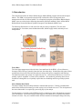
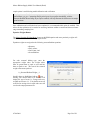
The following illustrates the overall work flow and processing components. The four main
components are: forest data, moose habitat data model, habitat supply model, and analysis and
interpretation.
Forest Data
The forest data component provides the basic forest attributes for the HSM. A Forest Resource
Inventory (FRI) GIS layer generally forms the base forest data layer. It should describe general forest
conditions such as non-forested and forested areas along with species composition and stand age.
The initial forest data may consist of a single time step (i.e., current forest land base) or a series of
spatially explicit ““snapshots”” of future forest conditions. One method of generating future forest
conditions is through the use of spatially explicit harvest scheduling and forest growth projection
tools.
Moose Habitat Data Model
The moose habitat data model helps maintain a standard data structure. Utilizing a standard data
model allows different forest data types with varying levels of detail to be used. The development of
the moose data model is a required pre-processing step by the analyst.
The data model is a spatially explicit ESRI shape file containing two basic field attribute categories:
static and dynamic. As the first category name suggests, static attributes are attributes that remain
constant over time. They are considered stable because natural non-catastrophic changes that may
07/06/2006
Page 3 of 28
Moose Habitat Supply Model User Manual (Draft)
occur are minimal over the short-term. Static attributes include water, wetlands, non-forested shrub
sites, non-forested unproductive sites and a forested sites moisture regime. The following table
provides a description of the required static attribute fields.
Attribute (site type)
Water
Wetland
Shrubs
Treed muskeg and
treed rock
Moisture regime
Unique polygon
Identifier
Name
Field Specifications
Type
Range
Field Description
NP_WATER
number
0 or 1
Identifies all rivers, small lakes (< 260 ha)
and small bays on large lakes. All water
polygons are assigned a code value of 1.
NP_WETLAND
number
0 or 1
Identifies all wetland types that represent
aquatic feeding sites*. All wetland sites are
assigned a code value of 1.
0 or 1
Identifies all non-forested sites that support
either willow (salix sp.) or redosier dogwood
(Cornus sericea) shrub types. All shrub sites
are assigned a code value of 1.
0 or 1
Identifies all treed muskeg and treed rock
sites. These areas are not considered to be
part of the productive forested land base.
Based on the Manitoba Conservation
productivity list, these sites fall within the
700 and 710 code series. All identified sites
are assigned a code value of 1.
NP_SHRUB
NP_UNPROD
MOISTURE
HSM_ID
number
number
character
number
DRY
FRESH
MOIST
WET
VERY WET
1,2,3……n
Identifies the moisture regime class for
forested stands. All forested stands must be
assigned a valid moisture regime class label
(see field range cell).
Forest data sets lacking a moisture regime
label can derive a moisture regime class from
species composition and site class which are
aided by available supplementary data
sources such as landform and\or indicator
plants
Unique numeric value assigned to all
polygons. For source data derived from
coverages, this field can be populated from
the coverages internal ID field. For source
data derived from a shape file, this field can
be populated from the shape files FID field.
* Aquatic feeding sites are locations where moose consume large quantities of emergent and submergent
aquatic vegetation (e.g. pondweed {Potamogeton spp.}and yellow pond lily {Nuphar microphyllum}) during
summer months.
Dynamic attributes refer to attributes that change over time due to forest succession, forest
management activities, or natural disturbances (if modelled). Dynamic attributes only apply to
forested stands. Attributes include stand strata, stand age, percentage of conifer species within the
stand and its seral stage class. The following table provides a description of all required dynamic
attribute fields.
07/06/2006
Page 4 of 28
Moose Habitat Supply Model User Manual (Draft)
Field Specifications
Attribute (site type)
Name*
Type
Field Description
Range
The stand strata label is user defined. The
strata label represents a classification
scheme based on species composition and
reflects stands with similar species types.
Strata
STRATA_0
character
User Defined
Stand Age (yrs)
AGE_0
number
0 to 999
Identifies the age of each stand.
0 to 100
Defines the total percentage of all conifer
species within the stand. A pure conifer
stand would be assigned a value of 100. A
pure hardwood stand would be assigned a
value of 0
Percentage of conifer (%)
SWD_0
number
The strata label is not directly used by the
HSM model. It is required for assigning the
seral stage label and\or crown closure
values. See Appendix 1 for an example of a
simple strata classification scheme.
Defines the stands crown closure. A mature
stand where tree crowns block nearly all
sunlight from hitting the forest stand floor
would be assigned a crown closure value of
100.
Crown closure (%)
CC_0
number
0 to 100
Forest datasets lacking crown closure
values can be derived from field data (e.g.
permanent sample plots) or through expert
option. See Appendix II for several crown
closure curve examples.
Seral Stage
SSTAGE_0
character
Grass
Seedling
Sapling
Immature
Mature
Overmature
Defines the stands seral stage class. Each
forested stand must have a valid seral stage
class label (see field range cell).
The seral stage class is derived by defining
an appropriate age break point for each
strata. See Appendix 1 for an example of
age class break points for several forest
strata.
* All dynamic field names must contain an integer value to identify its inventory period. An inventory period
of 0 (zero), for example, represents the first inventory period or today’’s forest conditions (e.g., AGE_0).
Future forest conditions are designated by the inventory period (e.g., AGE_1, AGE_2, and AGE_3). A user
defined HSM model parameter defines the time step for each inventory period (e.g., 5 years).
Habitat Supply Model (HSM)
The HSM generates potential habitat suitability indices for each inventory period along with simple
summary statistics and maps for various habitat quality indices and forest parameters. The models
graphical user interface (GUI) manages all model inputs within user defined scenario folders. All
required parameters are entered or modified through the model’’s GUI.
07/06/2006
Page 5 of 28
Moose Habitat Supply Model User Manual (Draft)
The two main model components are: the moose data model (discussed in the previous section) and
model input parameters. The moose data model describes the study area’’s current and future forest
conditions. The data model is spatially explicit which allows for an assessment of current and\or
future potential moose habitat under various land use planning scenarios. The model parameters for
example, relate important forest attributes (e.g., seral stage) to moose habitat suitability, defines the
spatial relationships between habitat and their proximity to specific land features (e.g., areas close to
water) and home range size (e.g., 2,500 ha). The analyst can modify all model parameters to suit a
specific region. The model’’s default parameter settings are regionally specific to the Mid Boreal
Uplands Ecoregion in western Manitoba.
The HSM is raster based and generates suitability index and forest parameter output files formatted as
ESRI grids.
Analysis and Interpretation
Most modelling exercises involve multiple simulation runs. Multiple runs result from the two
feedback loops shown above: model parameter refinement and forest planning refinement. The
model parameter refinement feedback loop occurs during the model validation and calibration stage.
It generally involves adjusting specific model parameters (e.g., shifting a crown closure suitability
index curve) and is usually linked to a sensitivity analysis. A sensitivity analysis is performed to
determine which model parameters are the least sensitive to adjustment. The forest planning
refinement loop is related to modifications to your forest management activities. This may involve,
for example, an adjustment to your harvest schedule to help maintain a specific level of potential
moose habitat in a particular area. Any modification to the forest data model requires the analyst to
rebuild the moose data model to rerun the HSM.
1.1 Program Requirements and Structure
The HSM package was designed to run within ArcInfo’’s workstation environment and is structured
around the Arc Macro Language (aml). Users interact with the program through a series of custom
menus. It requires Arc/Info Workstation and the associated Grid module to run.
1.2 Program File Structure
Due to the complex set of input and output files, the program maintains a rigid file structure for
storing both input and output files. A complete description of all input and output files and their
locations are described in later sections.
The HSM program maintains a rigid file program structure. The following table describes the core
program file folders:
Folder Name
Description
Program
Menu and start-up program file (i.e., hsmMoose.exe).
General
Workspace for all spatial input files.
Shared_Amls
Species
07/06/2006
Shared program (aml) files.
Species level program (aml) and input files. Input files are stored within individual
scenario folders (e.g., scen0) as sub-folders within the models folder. Once created, a
scenario folder stores all required input parameter files.
Page 6 of 28
Moose Habitat Supply Model User Manual (Draft)
2.0 Setup
The complete program package and sample dataset for the HSM is included within the main
Setup.exe install file. To install:
1) Double click the Setup.exe file.
2) Select all default values unless a different
program installation location is required.
The user should avoid placing the programs root
folder in a location that creates a long path string.
Long path strings can cause problems when
running the model due to limitations within
ArcInfo.
To uninstall, use the Add/Remove Programs
option on the Control Panel.
Arc 9.1 users will require a patch to fix an ARCPRESS related bug. The patch is included in
the programs root folder within the arc91_arcpress_patch sub folder or it can be downloaded
from the ESRI Support Center website: http://support.esri.com.
Sample Dataset
The sample data model is provided to help
users become familiar with the model’’s
standard data structure. It also facilitates the
ability to easily execute the model using
default model parameters and examine
model output and formats.
The sample data model is located within the
general workspace (i.e., C:\mmf_hsm\V1\
general\shape.shp).
The data model contains forest projection
snapshots every ten years for 150 years.
Each inventory period represents a five year
planning time step, therefore the planning
periods are in increments of two (i.e.,
planning period 0,2,4,6, etc.).
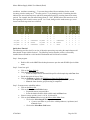
The following table is a subset of the sample.shp data model to help illustrate the required stand
attributes for 6 polygons. Dynamic stand attributes are shown for three of the six polygons for two of
the 15 inventory periods. Attributes containing ““_0”” represent the forests base (current) stand
07/06/2006
Page 7 of 28
Moose Habitat Supply Model User Manual (Draft)
SWD_2
NP_WATER
NP_SHRUB
NP_UNPROD
NP_OWATER
0
0
0
0
1
0
0
0
0
0
0
0
0
0
1
0
0
0
0
0
0
0
0
1
0
0
0
1
93
60
0
50
0
0
0
0
0
0
NAT_SWD4
91
50
100
NAT_HWD2
91
60
0
OVERMATURE
NAT_HWD1
103
MATURE
NAT_SWD4
101
50
100
OVERMATURE
LP_HWD2
0
10
0
OVERMATURE
NP_WETLAN
D
CC_2
0
0
SSTAGE_2
AGE_2
0
0
STRAT_2
SWD_0
0
SSTAGE_0
CC_0
NAT_HWD1
AGE_0
STRAT_0
conditions. Attributes containing ““_2”” represent the predicted forest conditions for the second
inventory period or tenth year (2nd inventory period * 5 yrs planning period). Examining the table
indicates the successional trajectory and forest management activities occurring between inventory
periods. For example, the sixth stand listing (Strata_0 = NAT_HWD2) shows this stand was cut at
the beginning of the second inventory period. As a result, changes to the stands strata, age, crown
closure and seral stage class have occurred.
MATURE
0
0
0
0
0
GRASS
0
0
0
0
0
Quick Start Tutorial
The following provides a brief overview of the major processing steps using the sample data model.
More details are provided in Section 3. The following section assumes you have successfully
installed the model and have valid ArcInfo Workstation and Grid licences available.
Step 1: Start program.
x
Double click on the MMF Hsm desktop shortcut to open the main Wildlife Species Main
menu.
Step 2: Create base grid.
x Click on the Base Grid tab.
x Click the Select Shape File button
o Select the sample moose data model shape file called sample.shp and Close form.
x Set the base grid cell size to 25m.
x Click on Continue to display the HSM Process Base Grid Window form
o Click on the Run button to begin the shape file to grid conversion process.
o Close the form when the grid processing is completed.
Step 3: Generate moose suitability indices
x Click on the Moose tab.
x Click on the Set Scenario Folder button.
o Expand the moose program folder.
o Select the default scenario folder called scen0 and Close form
x Select inventory periods (year) 0, 10, 20, 30, 40 and 50.
x Click on the Continue button to open the Moose Main Menu form
o Click on the Select Output Workspace button
x Create a new folder on your c drive called quicktour (c:\quicktour) and
Close the form.
o Click on the Select Base Grid button.
07/06/2006
Page 8 of 28
Moose Habitat Supply Model User Manual (Draft)
x
o
o
o
o
Select the sample_g grid you created in Step 2 and click on the Apply
button to close the form.
Click on the Proximity and Home Range button.
x Select the Home Range Zone Matrix tab
x Select the 4 by 4 (16 zonal layers) option in the Matrix Size pane.
x Click on the Save Parameters button to save your changes.
x Close the Moose Proximity and Home Range Menu form.
Click on the View Input Files button
x Click on the Home Range button to view the proximity and home range
parameters file contents. Check to ensure the
HOME_RANGE_MATRIX variable is equal to 4.
x Close the Moose File Viewer form.
Click on the Continue button to open the HSM Process Window form.
x Click on the Run button to begin processing. The processing time is
dependent on the size of your forest, the number of inventory steps, the
home range matrix size and your computers processing speed.
x Close the form when the model simulation has finished processing.
x Close the Moose Main Menu form.
Open ArcCatalog and navigate to the output folder (i.e., c:\quicktour).
x Expand the habitat_grids workspace list. This workspace should contain
a series of habitat suitability indices (grids) for years 0, 10,20,30,40, and
50.
x Highlight one of the suitability index grids for summer cover (i.e.,
cov_s_0). To view, select the Preview tab.
x Select the blue i icon on the top menu. Clicking in the preview pane
displays the suitability index value within the Identify Results window.
A zero value represents unsuitable summer cover habitat. A value of 100
represents suitable summer cover habitat.
x Close all forms and exit ArcCatalog.
Step 4: Generate moose suitability maps and summary statistics
x Click on the HSM Maps tab.
x Click on the Select Output Workspace button
o Select the output folder directory where you have saved your simulation
results (i.e., c:\quicktour). Select Ok to close form.
x Click on the Select Base Grid button.
o Select the sample_g grid from the Grid file list window and select Apply to
close the form.
x Click on the Continue button to open the HSM Map Window form.
o Click on the Run button to begin possessing.
o Close the form when the HSM map and summary statistics processing has
been completed.
x Exit the HSM program
o Clicking on the Close button to exit.
x With Windows Explorer, navigate to your output folder (i.e., c:\quicktour)
o Two new folders called maps and maps-hi-low have been added to your
output folder.
07/06/2006
Page 9 of 28
Moose Habitat Supply Model User Manual (Draft)
Double click on the maps folder to display its contents. Double click on a
jpg file to view. Scroll down and double click on the image file called
moose_poster.jpg to view a compiled poster of habitat suitability index maps.
Using Windows Explorer, navigate back to your output folder (i.e., c:\quicktour)
o Several new habitat suitability and forest parameters summary files
(moose_*.dbf) have been added to the output folder. Each file is a summary
of the critical habitat elements for the full simulation period.
o
x
07/06/2006
Page 10 of 28
Moose Habitat Supply Model User Manual (Draft)
3.0 Running the Moose Habitat Supply Model
The HSM menu system is initiated by double clicking on the MMF Hsm shortcut located on your
desktop. The shortcut is linked to the program file located within the \program\bin installation
directory.
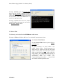
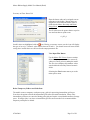
The program begins by displaying the main
Wildlife Species Main Menu form, which
appears in the upper left corner of your screen.
Each tab provides access to a specific
processing task.
The Base Grid tab generates the required base
input grid from a user-defined input shape file.
The base grid module only needs to be
performed once; however, if the input shape
file is modified, the base grid must be
recreated.
The Moose tab provides access to the setup
and execution forms for generating habitat
suitability indices.
The HSM Maps tab generates suitability
indices summary statistics and maps from
your model outputs.
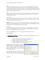
3.1 Base Grid Tab
The following section describes the Base Grid tab form.
Selecting the Base Grid tab displays the Base Grid tab
form. The Shape File Input Location pane identifies
the input folder location. The input shape file is
selected by clicking on the Select Shape File button.
Set the output grid cell size from the Base Grid Cell
Size track bar.
The Output Grid Name displays the grid file that will
be created. The grid file name is limited to 9
characters. If the input shape file contains more than
nine characters (e.g., longfilename.shp), the file name
is renamed using the first nine characters with an
additional ““_g”” appended to the file name (i.e.,
longfilen_g).
07/06/2006
Page 11 of 28
Moose Habitat Supply Model User Manual (Draft)
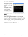
Selecting Continue opens the Process Form
menu with an ArcInfo command window
viewer. The Process Form contains a preview
of the input shape file, the output grid name
and its location. Click on the Run button to
start the base grid processing.
Selecting the Close button closes the ArcInfo
command window and returns the user back to
the Base Grid Attribute menu.
3.2 Moose Tab
The following section describes the HSM Moose module menus.
Selecting the Moose tab displays the first of several model input parameter forms.
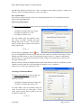
Set Scenario Folder Button
The Set Scenario Folder button opens the Browse
for Folder form.
All input parameters are stored within a user
defined scenario folder. Model parameters for
each species are written to text files and stored
within a scenario folder. The name of the scenario
folder is user-defined and must reside within the
moose folder. For example, a scenario consists of
a folder located within the moose folder with a
user-defined
label
of
scen0
(i.e.,
C:\mmf_hsmV1\species\models\
moose\scen0)
and contains all model parameter files.
07/06/2006
Page 12 of 28
Moose Habitat Supply Model User Manual (Draft)
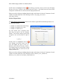
Selecting an existing scenario folder will load all model
parameters into memory. To create a new scenario
folder, highlight the moose folder and click on the Make
New Folder button. Right click on the newly created
folder and select the Rename option to assign a new
scenario name. Clicking the Ok button will populate the
scenario folder with all required input files. A Status
form is displayed listing the files created and their
location. Selecting the Close button returns you back to
the Wildlife Species Main Menu.
Scenario files can also be loaded from the File -> Load
Scenario menu. The Scenario Folder File Listing form
is displayed (not shown) with a summary of all
parameter files loaded into memory.
You can easily create multiple scenarios by first creating a base case scenario from the Set
Scenario Folder button. With Windows Explorer, copy and rename your base case scenario
folder and then reload the newly created scenario folder and modify as required.
The Make New Folder button on the Browse For Folder menu has a quirky behaviour of
sometimes not appearing on the form. Closing and reopening the form or restarting the program
will usually cause the button to reappear.
Clicking the Continue button on the Moose tab opens the Moose Main Menu form.
The output folder location is set with the Select
Output Workspace button. The selected folder
path is displayed within the Output Location
pane.
The base grid input raster file is set using the
Select Base Grid button. The Base Grid
Selection Menu (not shown) is displayed with a
listing of all inventory base grids found within
the GENERAL workspace. Readers are referred
to the Base Grid tab section, for more
information on creating your base grid. The
selected grid is displayed in the Base Grid pane.
The Model Configuration Pane holds model
configuration buttons for accessing the models
input parameters and file viewer forms.
07/06/2006
Page 13 of 28
Moose Habitat Supply Model User Manual (Draft)
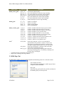
Global Variables Button
The Global Parameter Menu displays required fields for
the various model components. Except for the Inventory
Time Step and Age Class Period parameters, default
field names are displayed in brackets beside each field
label. It is recommended you build your initial input
layer using the default field names shown here.
Inventory Time Step (years):
The years between each harvest period.
Age Class Period (years):
The period in years that defines the age class.
The remaining parameters access the base grids value attribute table (vat).
Water (np_water):
The field name for identifying water polygons. This field should identify all rivers, small lakes (<
260 ha) and small bays on large lakes. In order to include smaller bays, it’’s recommended the larger
lake polygon be partitioned to allow for the smaller bays to be modelled as distinct zones. Stands
adjacent to these water bodies will be assigned a summer food and summer cover bonus suitability
value (see section Proximity to Water Bonus Tab below for more information).
Shrub (np_shrub):
The field name for identifying non-treed shrub sites that support willow or dogwood as their primary
shrub type.
Wetlands (np_wetlands):
The field name for identifying wetlands which support aquatic vegetation.
Treed Muskeg and Treed Rock (np_unprod):
The field name for identifying treed muskeg and rock outcrops. These areas represent treed areas not
included within the productive forest land base (i.e., Manitoba Conservation 700 and 710 productivity
code series).
Open Water (np_owater):
The field name for identifying all open water polygons. These areas are excluded from the home
range smoothing statistic.
Moisture Regime
The field name for identifying moisture regime classes for forested stands.
07/06/2006
Page 14 of 28
Moose Habitat Supply Model User Manual (Draft)
Strata
Select one of the fields that represent a stand’’s strata type. For example, strata by default, is the
prefix that represents fields that identify a stand’’s strata. Each field containing the prefix strata will
also have an associated inventory period (e.g., strata_0). The inventory value represents the inventory
period and not the inventory year. To determine the inventory year, multiply the inventory period by
the inventory time step (specified above).
Age
Select one of the fields that represent a stand’’s age. For example, age is the prefix that represents the
fields that identify a stand’’s age. Each field containing the prefix age will also have an associated
inventory period (e.g. age_0).
Crown Closure
Select one of the fields that represent the stand’’s crown closure. For example, cc is the prefix that
represents the fields that define a stand’’s crown closure. Each field containing the prefix cc will also
have an associated inventory period (e.g., cc_0).
Softwood
Select one of the fields that represent a stand’’s softwood percentage. For example, swd is the prefix
that represents the fields that identify a stand’’s softwood percentage. Each field containing the prefix
swd will also have an associated inventory period (e.g., swd_0).
Seral Stage
Select one of the fields that represent a stand’’s seral stage. For example, sstage is the prefix that
represents the fields that identify a stand’’s seral stage. Each field containing the prefix sstage will
also have an associated inventory period e.g., sstage_0).
Click the Save Settings button to save your changes to the global_parameters.txt file.
SI Curves Button
The Suitability Curves (SI) Menu form defines the reclassification or standardization curves for the
following variables:
x
x
x
x
x
Variable 1: Summer and winter forage by percent conifer cover,
Variable 3: Summer and winter forage by crown closure,
Variable 4: Summer cover by percent conifer,
Variable 6: Summer and winter cover by crown closure, and
Variable 7: Winter cover by percent conifer cover
Selecting an SI variable populates the SI curve
inflection point fields. Each curve is defined by a
series of x.y points. A maximum of six points are
allowed. The model performs a linear interpolation
between each point; therefore you only need to enter
the main inflection points.
Curve adjustments are made by editing the x and y
fields in the Chart Values pane. The curve displayed
in the Chart Area and Curve File Format panes is
07/06/2006
Page 15 of 28
Moose Habitat Supply Model User Manual (Draft)
automatically updated to reflect the new value. All numeric values must be greater or equal to zero
with no x-values exceeding 100 and no y-values exceeding 1.
Save All Edits Button
Saves all curve edits to the moose.rmp curve definition parameter file. To exit without saving your
edits click on the Close button.
Non-Forested Sites Button
The Moose Non-forested Menu form sets the non-forested HSI classification parameters for the
following variables:
x Variable 8: Summer and winter forage,
x Variable 9: Summer cover, and
x Variable 10: Winter cover
For each variable, enter the suitability index
(SI) values for shrub, wetlands and treed
muskeg and treed rock sites. The SI values
must be greater than or equal to zero and less
than or equal to one:
0 ” SI ” 1
Invalid values are highlighted with an
icon.
An error is highlighted in the above figure since the value entered is outside the valid range of values.
Placing your mouse cursor over the icon will display the type of error (i.e., Numeric value must be
between 0 and 1). You should correct all errors before saving since invalid values are still saved to
the output parameter file.
Edits are saved by clicking on the Save button located on the bottom of each tab. Parameters for each
variable are stored within one of the following files: nonprod_cover_ summer.txt,
nonprod_cover_winter.txt or nonprod_food.txt.
Seral Stage Classification Button
The Moose Seral Stage Menu form sets the seral
stage HSI classification parameters for the
following variables:
x Variable 2: Summer and winter forage, and
x Variable 5: Summer and winter cover,
For each variable, enter the suitability index (SI)
values for each of the six seral stages. The SI
values must be greater than or equal to zero and
less than or equal to one:
0 ” SI ” 1
07/06/2006
Page 16 of 28
Moose Habitat Supply Model User Manual (Draft)
icon. Placing your mouse cursor over the icon will display
Invalid values are highlighted with an
the type of error (i.e., Numeric value must be between 0 and 1). You should correct all errors before
saving since invalid values are still saved to the output parameter file.
Edits are saved by clicking on the Save button located on the bottom of each tab. Parameters for each
variable are stored within one of the following text files: seral_stage_cover.txt or
seral_stage_food.txt.
Moisture Regime Button
The Moose Moisture Regime Menu form sets the moisture regime HSI classification parameters for
the following variables:
x Variable 11: Summer and winter forage,
x Variable 12: Summer cover, and
x Variable 13: Winter cover
For each variable, enter a suitability index
(SI) value for each of the five moisture
regimes. The SI values must be greater than
or equal to zero and less than or equal to
one:
0 ” SI ” 1
Invalid values are highlighted with an
icon. Placing your mouse cursor over the
icon will display the type of error (i.e.,
Numeric value must be between 0 and 1).
You should correct all errors before saving
since invalid values are still saved to the
output parameter file.
Edits are saved by clicking on the Save button located on the bottom of each tab. Parameters for each
variable are stored within one of the following text files: moisture_cover_summer.txt,
moisture_cover_winter.txt or moisture_food_summer.txt.
07/06/2006
Page 17 of 28
Moose Habitat Supply Model User Manual (Draft)
Proximity and Home Range Button
The Moose Proximity and Home Range Menu form sets spatial parameters related to stand proximity
and home range zonal algorithms. All values are stored within the proximity_ distance.txt file.
Proximity Tab
Enter the distance (meters) for the adjustments of SI
values based on the proximity between foraging and
cover habitats in the Distance between foraging and
cover box.
This value defines the radius of a circular window
used to determine the windows maximum summer
food and summer cover SI value.
Enter the buffer distance (meters) to be used around all rivers, small lakes (< 260 ha) and small bays
in the Distance from a water body box. Both summer food and cover values falling within these
zones are assigned a bonus value due to there proximity to water.
For further information on these proximity values, readers should review the Adjustment of SIs
Based on Proximity between Foraging and Cover Habitats section of the Moose HSM document
(McNicol and Rudy, 2006).
Home Range Area Tab
Enter the area of the moose’’s home range.
The home range value is also expressed in
square kilometres (km2) along with its
equivalent radius (meters) distance.
This value defines the size of the home
range windows used in the home ranging
smoothing procedure.
07/06/2006
Page 18 of 28
Moose Habitat Supply Model User Manual (Draft)
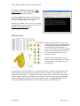
Home Range Zone Matrix Tab
Select if the home range smoothing summary statistics will utilize a 4 by 4 (16 zonal layers) or an 8
by 8 (64 zonal layers) matrix.
Home range values are computed from a
series of non-overlapping zonal grids.
An example of a single non-overlapping
zonal grid is illustrated in the Home Range
Parameters pane. Home range center points
are represented by black dots.
For example, by selecting a 4 by 4 matrix,
sixteen separate zonal layers will be used in
the home range smoothing process. Each
layer is slightly shifted resulting in each
zones centre points to be offset from center
points on the other zonal layers.
For each layer, the habitat values within each circular home range zone are averaged and assigned to
each zones centre point. The centroid values from each of the 16 layers are then combined to create a
single layer of the averaged SI values. Selecting an 8 by 8 matrix utilizes more zonal layers (64
layers), which in turn, results in a higher sampling intensity.
The home range smoothing approach selected here performs a systematic sample of locations across
the area of interest at the scale of an average moose home range as opposed to calculating an average
SI value for each cell.
This approach was selected because the computational time to calculate average SI values for each
cell was impractical and moose use their habitat at a much larger scale than that represented by a
single cell (i.e. 25m2).
Readers are referred to Plate 12 in Appendix 5 of the Moose HSM document for more information
regarding the home range smoothing approach used in this model.
Random Home Range Tab
By default, the first initial home range
zonal grid is anchored to the lower left
corner of the base grid. Each of the home
range zonal grids is then shifted from this
anchor point. As a result, the same sample
points (zone centre points) are used in the
home range summary statistics each time
the model is run.
The Generate Random Home Range
Layers option solves this problem by
randomly generating a new anchor point
each time the model is run. Using static
07/06/2006
Page 19 of 28
Moose Habitat Supply Model User Manual (Draft)
sample points is useful during model calibration and verification.
Sample points used in the home range process are stored within a point coverage called
\zones\home_rge_pts. Comparing sample point layers from separate simulations, with the
Generate Random Home Range layers option enabled, will help illustrate the differences in sample
point locations.
Once calibration and verification has been completed, it is recommended this option be enabled. This
allows for the replication of a scenario for assessing variations within a scenario and decreases home
range smoothing sampling bias.
Equation Weights Button
The Moose Equation Weights Menu form sets the HSM equation and water proximity weights. All
values are stored within the habitat_weights.txt file.
Equation weights are assigned to the following seasonal habitat equations:
x
x
x
x
Summer,
Early winter,
Late winter, and
Overall habitat
For each seasonal habitat type, enter the
appropriate weight value. The weight values
must be greater than or equal to zero and less
than or equal to one. The sum of the seasonal
weight value must equal one.
0 ” Seasonal Habitat Weight ” 1
Invalid values are highlighted with an
icon.
Placing your mouse cursor over the icon will
display the type of error (i.e., Forage and cover
weights must sum to 1!). You should correct all
errors before saving since invalid values are still
saved to the output parameter file.
07/06/2006
Page 20 of 28
Moose Habitat Supply Model User Manual (Draft)
Proximity to Water Bonus Tab
Enter the bonus values to be assigned to areas
adjacent to water bodies. Bonus values are
assigned to areas within the buffer zones as
defined in the Moose Proximity and Home
Range Menu.
The SI values must be greater than or equal to
zero and less than or equal to one:
0 ” SI ” 1
Invalid values are highlighted with an
icon. Placing your mouse cursor over the icon will display
the type of error (i.e., Numeric value must be between 0 and 1). You should correct all errors before
saving since invalid values are still saved to the output parameter file.
View Input Files Button
Use the Moose File Viewer form to examine
all model input parameters and to ensure all
values are correct prior to running the model.
The file viewer displays all parameter values
stored within the currently selected scenario
folder.
Selecting the Close button returns you to the
main species menu.
Delete Temporary Folders and Grids Pane
The model creates a temporary workspace (temp_grids) for processing intermediate grid layers.
Users have the option to delete the intermediate grids after each model simulation. Many of the
intermediate grid layers are stored as floating point grids and require a considerable amount of storage
space. If storage space is an issue or intermediate grid files are not needed it is recommended the
temporary workspace be deleted.
07/06/2006
Page 21 of 28
Moose Habitat Supply Model User Manual (Draft)
Once you have edited all required model
parameters click the Continue button to
open the HSM Process Window. The
Preview Pane lists the species name,
output path and the scenario’’s folder
location.
Selecting the Run button starts the
model process.
Model processing
results are displayed within the Arc\Info
Command Output viewer pane.
Selecting the Close button closes the
ArcInfo command window and returns
the user back to the Moose Main Menu.
Selecting the Close button on the Moose Main Menu form returns you back to the Wildlife Species
Main Menu form.
Moose Model Simulation Results
The model generates a suite of habitat suitability index (HSI) grids for each inventory period
modelled. The grid naming convention contains a prefix of the habitat type followed by the inventory
year (i.e., cov_s_10). An HSI traditionally consists of values ranging between zero and one with zero
suitability values indicating the potential for unsuitable habitat and suitability values of one indicating
the potential for suitable or optimum moose habitat. All HSI grids are rescaled to a range between 0
(unsuitable) and 100 (suitable). This rescaling process converts all output grids from a floating grid
format type to an integer grid type format which helps to substantially reduce storage space
requirements.
All output is stored within the user defined output folder. The following table lists the content of each
subfolder and illustrates all outputs for the tenth simulation year.
07/06/2006
Page 22 of 28
Moose Habitat Supply Model User Manual (Draft)
Folder Name
Grid Name
Description
habitat_season_grids
moose_10*
home_ear_10
home_late_10
home_sum_10
si_ear_10
si_lat_10
si_sum_10
Overall moose habitat quality
Early winter habitat layer after home range smoothing
Late winter habitat layer after home range smoothing
Summer habitat layer after home range smoothing
Early winter habitat prior to home range smoothing
Late winter habitat prior to home range smoothing
Summer habitat prior to home range smoothing
habitat_grids
cov_s_10
cov_w_10
food_s_10
food_w_10
Summer cover habitat
Winter cover habitat
Summer foraging habitat
Winter foraging habitat
habitat_variable_grids
v1_fd_10
v2_fd_10
v3_fd_10
v4_cov_10
v5_cov_10
v6_cov_10
v7_cov_10
v11_fd_10
v12_cov_10
v13_cov_10
Variable 1: Summer and winter forage by percent conifer
Variable 2: Summer and winter forage by seral stage
Variable 3: Summer and winter forage by crown closure
Variable 4: Summer cover by percent conifer
Variable 5: Summer and winter cover by seral stage
Variable 6: Summer and winter cover by crown closure
Variable 7: Summer cover by percent conifer
Variable 11: Summer and winter forage by moisture class
Variable 22: Summer cover by moisture class
Variable 13 Winter cover by moisture class
zones**
zone#_home
*
**
Home range zonal grid. A series of 16 zonal grids are
generated when a 4 by 4 matrix is selected. A series of 64
zonal grids are created if an 8 by 8 matrix is selected. Each
zonal grid is slightly shifted from the lower left anchor point.
cent#_home
Home range centroid grid. Centroids are derived from the
center point of each home range zone.
home_rge_pts Point coverage illustrating the sampling points used in the
home range smoothing process. Generated by combining all of
the home range centroid grids.
Calculated from the seasonal home range habitat layers.
Required for calculating home range statistics.
3.3 HSM Maps Tab
The HSM Maps module generates habitat snapshots and summary posters for a selected scenario.
Select Output Location:
Select the folder containing the model outputs from a
completed model simulation.
Base grid:
Select the base grid used for the specific run related to
the habitat grids you wish to process.
07/06/2006
Page 23 of 28
Moose Habitat Supply Model User Manual (Draft)
Selecting the Continue button opens the HSM
Map Window form. The Preview Pane lists the
folder source path and species name.
Selecting the Run button starts the model process.
Model processing results are displayed within the
Arc\Info Command Output viewer pane.
Selecting the Close button closes the ArcInfo
command window and returns the user back to the
Wildlife Species Main Menu form.
HSM Map Outputs
Summary outputs include a series of 8.5 x
11 image files displaying a suitability index
map and frequency histogram chart for the
various HSI and forest parameters. A
selected set of images are collected together
for the creation of a summary poster (24”” x
36””) for several habitat types or forest
parameter variables.
In addition to the map products, a set of
tabular summary tables (dBase file format)
are generated for each habitat type and
forest parameter.
All map images are stored within the user defined output folder. Both map frequency charts and
tabular statistics are generated using two different SI interval widths. The first SI interval type is
based on ten interval steps. The second interval type is based on three equal interval steps used for
defining a high-medium-low SI ranking system. The following table lists the content of the maps
subfolder and describes all outputs for the tenth simulation year. The maps-hi-low subfolder is
similar to the maps subfolder but is based on the high-medium-low SI ranking system.
07/06/2006
Page 24 of 28
Moose Habitat Supply Model User Manual (Draft)
Folder
maps
07/06/2006
Image file (*.jpg)
Description
moose_10
Overall moose habitat quality map
home_ear_10
Early winter habitat layer after home range smoothing map
home_late_10
Late winter habitat layer after home range smoothing map
home_sum_10
Summer habitat layer after home range smoothing map
moose_poster
Poster of seasonal habitat types for years 0,10,20,30 40,90,120,150
si_ear_10
Early winter habitat prior to home range smoothing map
si_lat_10
Late winter habitat prior to home range smoothing map
si_sum_10
Summer habitat prior to home range smoothing map
moose_si
Poster of seasonal habitat types for years 0,10,20,30 40,90,120,150
cov_s_10
Summer cover habitat map
cov_w_10
Winter cover habitat map
food_s_10
Summer foraging habitat map
food_w_10
Winter foraging habitat map
moose_forage_cover_poster
Poster of habitat types for years 0,10,20,30 40,90,120,150
v1_fd_10
Variable 1: Summer and winter forage by percent conifer
v2_fd_10
Variable 2: Summer and winter forage by seral stage
v3_fd_10
Variable 3: Summer and winter forage by crown closure
moose_var_set1_poster
Poster (set 1) of forest variable for years 0,10,20,30 40,90,120,150
v4_cov_10
Variable 4: Summer cover by percent conifer
v5_cov_10
Variable 5: Summer and winter cover by seral stage
v6_cov_10
Variable 6: Summer and winter cover by crown closure
v7_cov_10
Variable 7: Summer cover by percent conifer
moose_var_set2_poster
Poster (set 2) of forest variable for years 0,10,20,30 40,90,120,150
v11_fd_10
Variable 11: Summer and winter forage by moisture class
v12_cov_10
Variable 12: Summer cover by moisture class
v13_cov_10
Variable 13 Winter cover by moisture class
moose_var_set3_poster
Poster (set 3) of forest variable for years 0,10,20,30 40,90,120,150
Page 25 of 28
Moose Habitat Supply Model User Manual (Draft)
A set of three summary tables are generated for each interval type and stored with the user defined
output folder. The dBase formatted fields are described in the following table.
Files (*.dbf)
moose
moose_hab
moose_var
Moose_hilow
moose_hab_hilow
moose_var_hilow
Field
Description
SI
Suitability index label (e.g., summer, early, late)
SCENARIO
Name of the scenario. The base grid name is used as the scenario label.
YEAR
Simulation year (e.g., 0, 10, 20, 30…….).
MEAN_SI
The overall average SI value.
SI_0
Percentage of landscape with an SI value between 0 and 9*
SI_1
Percentage of landscape with an SI value between 10 and 19
SI_2
Percentage of landscape with an SI value between 20 and 29
SI_3
Percentage of landscape with an SI value between 30 and 39
SI_4
Percentage of landscape with an SI value between 40 and 49
SI_5
Percentage of landscape with an SI value between 50 and 59
SI_6
Percentage of landscape with an SI value between 60 and 69
SI_7
Percentage of landscape with an SI value between 70 and 79
SI_8
Percentage of landscape with an SI value between 80 and 89
SI_9
Percentage of landscape with an SI value between 90 and 99
SI_10
Percentage of landscape with an SI value equal to 100
SI
Suitability index label (e.g., summer, early, late)
SCENARIO
Name of the scenario. The base grid name is used as the scenario label.
YEAR
Simulation year (e.g., 0, 10, 20, 30…….).
MEAN_SI
The overall average SI value.
LOW
Percentage of landscape with an SI value between 0 and 33
MEDIUM
Percentage of landscape with an SI value between 34 to 66
HIGH
Percentage of landscape with an SI value between 67 to 100
* Interval ranges are based on an SI range of 0 - 100. All model output was re classed from the standard 0 –– 1 SI
range to a 0 –– 100 SI range to help minimize storage requirements.
07/06/2006
Page 26 of 28
Moose Habitat Supply Model User Manual (Draft)
Appendix 1: Sample Strata and Seral Stage Age Break Points
Strata
Composition
Seral Stage
Grass
Seedling
Sapling
Immature Mature Overmature
PTA
80-100% TA, 0-20%softwood
0-3
4-6
7 - 20
21 - 50
51 - 70
71+
MDE
80-100%TA,BP,WB, 0-20%
softwood
0-5
6 - 10
11 - 25
26 - 55
56 - 75
76+
0-5
6 - 10
11 - 25
26 - 55
56 - 75
76+
0-5
6 - 10
11 - 25
26 - 55
56 - 75
76+
0-5
6 - 15
16 - 35
36 - 70
71 - 100
101+
0-5
6 - 15
16 - 35
36 - 70
71 - 100
101+
51-79%hardwood,2149%softwood,Wsor BF or JP
l di
51-79%hardwood,21NBS 49%softwood,BS and TL
l di
51-79%softwood,21MWS 49%hardwood,WS or BF or JP
l di
51-79%softwood,21MBS 49%hardwood,BS and TL
l di
NWS
PJP
80-100% softwood, JP leading
0-5
6 - 15
16 - 30
31 - 65
66 - 80
81+
PWS
80-100%white spruce, WS or
BF leading
0-5
6 - 15
16 - 35
36 - 70
71 - 100
101+
UBS
80-100% softwood, BS and TL
leading moisture class D,F,M,V
0-5
6 - 15
16 - 35
36 - 70
71 - 100
101+
LBS
80-100% softwood BS and TL
leading , moisture class W
0-7
8 - 20
21 - 50
51-89
90 - 120
121+
07/06/2006
Page 27 of 28
Moose Habitat Supply Model User Manual (Draft)
Appendix 2: Sample Crown Closure Curves
The following illustrates several sample crown closure curves derived through empirical data
interpretation, allometric equations and expert opinion. Each curve represents the change in crown
closure over time for a specific stratum.
07/06/2006
Page 28 of 28