Download MPC in LabVIEW

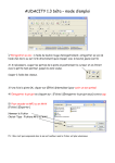
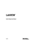
Creating and Implementing a
Model Predictive Controller
18
Traditional feedback controllers operate by adjusting control action in
response to a change in the output setpoint of a system, also called a plant.
Model predictive control (MPC) is a technique that focuses on constructing
controllers that can adjust the control action before a change in the output
setpoint actually occurs. This predictive ability, when combined with
traditional feedback operation, enables a controller to make adjustments
that are smoother and closer to the optimal control action values.
For example, consider a cruise control system in a car. This controller
adjusts the amount of gas sent to the engine. The amount of gas is based on
the following two values:
•
The velocity at which you set the cruise control system
•
The velocity of the car
The velocity of the car is based on the slope of the road along which the car
moves. Therefore, a change in slope, or disturbance, affects the velocity of
the car, which affects the amount of gas the controller sends to the engine.
Table 18-1 shows the terms this example uses, where k is discrete time.
Table 18-1. Example Terms and Definitions
Term
Physical Component
Variable
Cruise control system
—
Amount of gas sent to the engine
u(k)
Car
—
Plant output
Velocity of the car
y(k)
Plant output
setpoint
Velocity at which you set the
cruise control system
r(k)
Disturbance
Slope of the road
d(k)
Controller
Control action
Plant
© National Instruments Corporation
18-1
Control Design User Manual
Chapter 18
Creating and Implementing a Model Predictive Controller
Consider what happens when the slope of the road increases as the car
moves up a hill. This slope increase reduces the velocity of the car. This
decrease in velocity causes the controller to send more gas to the engine.
If the cruise control system is a traditional feedback controller, this
controller reacts to the disturbance only after the velocity of the car drops.
To match the output setpoint, this controller might increase the control
action sharply. This sharp increase can result in oscillation or even
instability.
If the cruise control system has predictive ability, this controller knows in
advance that the velocity of the car will drop soon. The controller might
obtain this information from sensors on the front of the car that measure the
slope of the road ahead. A feedback controller with this predictive ability is
called an MPC controller.
To match this predicted output setpoint, the MPC controller gradually
increases the control action as the car approaches the change in slope. This
increase can be smoother and more stable than the increase a traditional
feedback controller provides.
This chapter provides information about using the LabVIEW Control
Design and Simulation Module to design and implement a predictive
controller.
Note Refer to the labview\examples\Control and Simulation\Control
Design\MPC directory for examples that demonstrate the concepts explained in this
chapter. Refer to UKACC Control, 2006. Mini Symposia, as listed in the Related
Documentation section of this manual, for information about the algorithms these VIs use.
Control Design User Manual
18-2
ni.com
Chapter 18
Creating and Implementing a Model Predictive Controller
Creating the MPC Controller
You use the CD Create MPC Controller VI to create an MPC controller.
This VI bases the MPC controller on a state-space model of the plant that
you provide.
If you want to create an MPC controller for a transfer function model or a
zero-pole-gain model, you must first convert the model to a state-space model.
Note
Providing an accurate model improves the performance of the MPC
controller this VI creates. You can specify that the MPC controller
incorporates integral action to compensate for any differences between the
plant model and the actual plant.
You can use the State Estimator Parameters input of this VI to define a
state estimator that is internal to the MPC controller model. You also can
estimate model states by using the Discrete Observer function outside the
MPC controller. Refer to the Current Observer section of Chapter 15,
Estimating Model States, for more information about estimating model
states.
The following sections provide information about other parameters you use
to define the MPC controller.
Defining the Prediction and Control Horizons
When constructing an MPC controller, you must provide the following
information:
•
Prediction horizon (Np)—The number of samples in the future during
which the MPC controller predicts the plant output. This horizon is
fixed for the duration of the execution of the controller.
•
Control horizon (Nc)—The number of samples within the prediction
horizon during which the MPC controller can affect the control action.
This horizon is fixed for the duration of the execution of the controller.
The value you specify for the control horizon must be less than the value you specify
for the prediction horizon.
Note
© National Instruments Corporation
18-3
Control Design User Manual
Chapter 18
Creating and Implementing a Model Predictive Controller
Figure 18-1 shows these horizons.
Output Setpoint
Predicted Output
Past Output
Measurements
Control Action
Past Control
Action
k+Nc
k
k+Np
Time
Control Horizon
Prediction Horizon
Figure 18-1. Prediction and Control Horizons
In Figure 18-1, notice that at time k the MPC controller predicts the plant
output for time k + Np. Also notice that the control action does not change
after the control horizon ends.
At the next sample time k + 1, the prediction and control horizons move
forward in time, and the MPC controller predicts the plant output again.
Figure 18-2 shows how the prediction horizon moves at each sample time k.
Prediction
Horizon at Time k+1
Prediction
Horizon at Time k
k
k+1
k+Np k+Np+1
Time
Figure 18-2. Moving the Prediction Horizon Forward in Time
The control horizon moves forward along with the prediction horizon. Before
moving forward, the controller sends the control action u(k) to the plant.
Note
Because you cannot change the length of the prediction or control horizons
while the controller is executing, National Instruments recommends you set
the prediction horizon length according to the needs of the control problem.
In general, a short prediction horizon reduces the length of time during
Control Design User Manual
18-4
ni.com
Chapter 18
Creating and Implementing a Model Predictive Controller
which the MPC controller predicts the plant outputs. Therefore, a short
prediction horizon causes the MPC controller to operate more like a
traditional feedback controller.
For example, consider the cruise control system again. If the prediction
horizon is short, the controller receives only a small amount of information
about upcoming changes in the road slope and speed limit. This small
amount of information reduces the ability of the controller to provide the
correct amount of gas to the engine.
A long prediction horizon increases the predictive ability of the MPC
controller. However, a long prediction horizon decreases the performance
of the MPC controller by adding extra calculations to the control algorithm.
Because the control action cannot change after the control horizon ends,
a short control horizon results in a few careful changes in control action.
Consider the cruise control system again. After the control horizon ends,
the flow of gas to the engine remains constant, which means the velocity of
the car keeps changing until the velocity setpoint is reached.
If the control horizon is short, the controller attempts to meet the velocity
setpoint by changing the flow of gas only a few times and in small amounts.
A large control action in a short control horizon might overshoot the
velocity setpoint after the control horizon ends. However, as the controller
continues to execute, the velocity eventually settles around the setpoint.
Conversely, a long control horizon produces more aggressive changes in
control action. These aggressive changes can result in oscillation and/or
wasted energy. For example, if you set the control horizon of the cruise
control system too long, the cruise control system wastes gas due to
constant accelerating and decelerating.
You can reduce these aggressive changes by using weight matrices in the cost
function. Refer to the Specifying the Cost Function section of this chapter for information
about weight matrices.
Note
You provide horizon information by using the MPC Controller
Parameters parameter of the CD Create MPC Controller VI.
Specifying the Cost Function
The MPC controller calculates a sequence of future control action values
such that a cost function is minimized. You can specify weight matrices in
this cost function. These weight matrices adjust the priorities of the control
action, rate of change in control action, and plant outputs.
© National Instruments Corporation
18-5
Control Design User Manual
Chapter 18
Creating and Implementing a Model Predictive Controller
For specified prediction and control horizons Np and Nc, the MPC controller
attempts to minimize the following cost function J(k):
Np
J( k) =
Nc – 1
 [ ŷ ( k + i k ) – r ( k + i k ) ]
T
i = Nw
⋅ Q ⋅ [ ŷ ( k + i k ) – r ( k + i k ) ] +
Np
 [ Δu ( k + i k ) ⋅ R ⋅ Δu ( k + i k ) ] +  [ u ( k + i k ) – s ( k + i k ) ]
T
i=0
T
⋅
i = Nw
N ⋅ [u(k + i k) – s(k + i k)]
where
•
k is discrete time
•
i is the index along the prediction horizon
•
Np is the number of samples in the prediction horizon
•
Nw is the beginning of the prediction horizon
•
Nc is the control horizon
•
Q is the output error weight matrix
•
R is the rate of change in control action weight matrix
•
N is the control action error weight matrix
•
ŷ ( k + i k ) is the predicted plant output at time k + i, given all
measurements up to and including those at time k
•
r ( k + i k ) is the output setpoint profile at time k + i, given all
measurements up to and including those at time k
•
Δu ( k + i k ) is the predicted rate of change in control action at time
k + i, given all measurements up to and including those at time k
•
u ( k + i k ) is the predicted optimal control action at time k + i, given
all measurements up to and including those at time k
•
s ( k + i k ) is the input setpoint profile at time k + i, given all
measurements up to and including those at time k
You specify soft constraints Q, R, and N by using the MPC Cost Weights
parameter of the CD Create MPC Controller VI. Refer to the Implementing
the MPC Controller section of this chapter for information about
specifying r ( k + i k ) and s ( k + i k ) . The CD Implement MPC Controller
VI calculates the values of u ( k + i k ) , Δu ( k + i k ) , and ŷ ( k + i k ) .
Control Design User Manual
18-6
ni.com
Chapter 18
Creating and Implementing a Model Predictive Controller
Specifying Constraints
In addition to weight matrices in the cost function, you can specify
constraints on the parameters of an MPC controller. Remember that weight
matrices adjust the priorities of the control action, rate of change in control
action, and plant outputs. Constraints are limits on the values of each of
these parameters.
Use the CD Create MPC Controller VI to specify constraints for a
controller. You can specify constraints using either the dual optimization or
the barrier function method. The following sections describe each of these
two methods.
Note You also can update the constraints of a controller at run time. Refer to the Modifying
an MPC Controller at Run Time section of this manual for information about updating a
controller at run time.
Dual Optimization Method
Use the Dual instance of the CD Create MPC Controller VI to set
constraints using the dual optimization method. You can specify these
constraints in the MPC Constraints (Dual) parameter of the CD Create
MPC Controller VI.
The dual optimization method specifies initial and final minimum and
maximum value constraints for the control action, the rate of change in
control action, and the plant output. Use these constraints to represent
real-world limitations on the values of these parameters.
For example, consider the cruise control system again. In this example,
the control action, or the amount of gas provided to the engine, is
unconstrained. In reality, however, cars can send only a certain amount of
gas to the engine at once. You can design an MPC controller to take this
constraint into account, which is equivalent to placing a hard constraint on
the maximum value of the control action. Additionally, the road might have
speed limits at certain intervals. If you know these limits in advance, you
can specify that the car cannot exceed the speed limits. This specification
is equivalent to placing hard constraints on the maximum value of the plant
output.
When you use the dual optimization method, all constraints are weighted
equally and above any cost weightings you specify. For example, in the
cruise control system, the MPC algorithm places equal emphasis on trying
not to exceed the specified maximum amount of gas or the specified
maximum velocity. If you also specify an output error weighting, the
© National Instruments Corporation
18-7
Control Design User Manual
Chapter 18
Creating and Implementing a Model Predictive Controller
algorithm prioritizes the control action and plant output constraints over the
output error weighting. In other words, the algorithm tries not to exceed the
specified amount of gas or the specified maximum velocity, even if meeting
these constraints results in a large difference between the desired and actual
velocity of the car. When you use the dual optimization method, the MPC
algorithm adjusts the controller such that the specified constraints are never
exceeded.
Because all constraints are weighted equally when you use the dual
optimization method, you cannot reflect differences in cost or importance
for different parameters. For example, suppose you want to build a
controller that maintains the car at a specific velocity. You want to prioritize
minimizing the output error above meeting any other constraints. With the
dual optimization method, you cannot specify this priority. Similarly, if you
have two conflicting constraints, the controller cannot prioritize one over
the other. If you want to prioritize the constraints and cost weightings for a
controller, use the barrier function method instead of the dual optimization
method. Refer to the Barrier Function Method section of this chapter for
more information about the barrier function method.
Refer to the CDEx MPC with Dual Constraints VI, located in the
labview\examples\Control and Simulation\Control
Design\MPC directory, for an example of using the dual optimization
method to set constraints for a controller. Refer to the CDEx MPC Dual vs
Barrier Constraints VI in this same directory for a comparison of the dual
optimization and barrier function methods.
Refer to Nonlinear Programming, as listed in the Related Documentation
section of this manual, for more information about the dual optimization
method.
Barrier Function Method
Use the Barrier instance of the CD Create MPC Controller VI to set
constraints using the barrier function method. You can specify these
constraints in the MPC Constraints (Barrier) parameter of the CD Create
MPC Controller VI.
Like the dual optimization method, the barrier function method specifies
initial and final minimum and maximum value constraints for the control
action, the rate of change in control action, and the plant output. However,
the barrier function method also associates a penalty and a tolerance with
each of these constraints. The penalty on a constraint specifies how much
the MPC algorithm attempts to avoid reaching the constrained value. The
tolerance specifies the distance from the constrained value at which the
Control Design User Manual
18-8
ni.com
Chapter 18
Creating and Implementing a Model Predictive Controller
penalty becomes active. By specifying penalties on constraints, you can
prioritize the constraints and cost weightings of a controller.
Relationship Between Penalty, Tolerance, and Parameter
Values
If the distance between a parameter value z and its constrained value zj is
greater than or equal to the tolerance tolj, the penalty Pj is 0. The penalty
becomes active when z reaches zj – tolj, if zj is a maximum constraint,
or zj + tolj, if zj is a minimum constraint. The penalty then increases
quadratically as z approaches zj. When z equals zj, that is, when the
parameter value reaches the constrained value, Pj equals the specified
penalty constant pj. If z exceeds the constrained value, the penalty
continues to increase quadratically.
pmax
Penalty, Pmax
Figure 18-3 illustrates this behavior for a maximum constraint.
0
zmax
zmax–tolmax
Parameter Value, z
Figure 18-3. Penalty Profile for Parameter z with Maximum Constraint zmax
For example, consider a plant output y with a maximum constraint ymax,
tolerance ytol, and a penalty constant pmax of 5. Table 18-2 shows how the
penalty P increases as y approaches ymax.
Table 18-2. Increasing Penalty as a Function of Plant Output
Value of y
© National Instruments Corporation
Value of P for pmax = 5
y ≤ ( y max – y tol )
0
( y max – y tol ) < y < y max
0 < P < 5. The value of P increases
quadratically between 0 and 5.
18-9
Control Design User Manual
Chapter 18
Creating and Implementing a Model Predictive Controller
Table 18-2. Increasing Penalty as a Function of Plant Output (Continued)
Value of y
Value of P for pmax = 5
y = y max
5
y > y max
P continues increasing quadratically.
Consider again the cruise control system. Suppose the speed limit in an area
is 70 miles per hour. You therefore specify a maximum constraint of
71 miles per hour on the velocity of the car. Also suppose you impose a
penalty constant of five on this constraint. The penalty specifies the priority
the MPC algorithm places on keeping the velocity below 71 miles per hour.
If you specify a tolerance of five miles per hour on this constraint, the
tolerance range begins at 66 miles per hour. The penalty on the maximum
output constraint therefore becomes active when the velocity of the car
reaches 66 miles per hour. The penalty then increases from 0 to 5 over a
tolerance range of five miles per hour.
If you reduce the tolerance to two miles per hour, the penalty on the
maximum output constraint becomes active when the car reaches 69 miles
per hour. The penalty then increases from 0 to 5 in a shorter velocity
interval than before. In this case, the MPC algorithm responds to the
penalty and almost immediately tries to prevent the velocity from
increasing above 69 miles per hour. Because the penalty profile is steeper
than in the previous case when the tolerance was five, the MPC algorithm
has a shorter interval in which to prevent the velocity from exceeding the
constrained value.
Prioritizing Constraints and Cost Weightings
Remember that all constraints you specify using the dual optimization
method are weighted equally and above any cost weightings you specify.
With the barrier function method, you can prioritize the constraints against
each other and against any cost weightings you specify. When an MPC
algorithm recognizes that the penalty on a constraint is active, the algorithm
incorporates the penalty in the cost function and adjusts the control action
accordingly. For each constrained variable, the MPC algorithm must
balance the penalty with any cost weightings.
Control Design User Manual
18-10
ni.com
Chapter 18
Creating and Implementing a Model Predictive Controller
The following expression illustrates this behavior in the case of a maximum
constraint.
2
2
p zmax [ ( z max – tol max ) – z ] + ( z – z sp ) q ;z ≥ ( z max – tol max )
where
•
p zmax is the penalty constant for zmax
•
zmax is the maximum constraint on z
•
tolmax is the tolerance for zmax
•
z is the value of the control action or of the plant output
•
zsp is the setpoint value of z
•
q is the cost weighting on z
Note Refer to the Specifying Input Setpoint, Output Setpoint, and Disturbance Profiles
section of this chapter for information about providing setpoint information for a
controller.
When z is the control action, this expression becomes:
2
2
p Δumax [ ( Δu max – tol max ) – Δu ] + ( Δu ) r ; Δu ≥ ( Δu max – tol max )
where
•
p Δumax is the penalty constant for Δu max
•
Δu max is the maximum constraint on Δu
•
tolmax is the tolerance for Δu max
•
Δu is the value of the rate of change in control action
•
r is the cost weighting on Δu
The first term in the previous expression represents the cumulative effect of
the penalty. The second term represents the cumulative effect of the cost
weightings.
© National Instruments Corporation
18-11
Control Design User Manual
Chapter 18
Creating and Implementing a Model Predictive Controller
Consider again the cruise control system in which ymax is 71 miles per hour,
with a penalty constant of five and a tolerance of five miles per hour.
Suppose the desired plant output is 70 miles per hour, and the output error
weighting is one. If the velocity of the car is 60 miles per hour, the MPC
algorithm attempts to increase the velocity to 70 miles per hour, thereby
reducing the output error. When the velocity of the car reaches 66 miles per
hour, the penalty on ymax becomes active. Because the penalty constant is
significantly greater than the output error weighting, the MPC algorithm
prioritizes the output constraint above the output error. Therefore, the
controller attempts to reduce the velocity of the car to a level above but
close to 66 miles per hour. Suppose instead that the output error weighting
is 100. Because the output error weighting is significantly greater than the
penalty constant, the MPC algorithm prioritizes the output error above the
plant output. Therefore, the controller attempts to increase the velocity of
the car to a level closer to 70 miles per hour, despite the active penalty on
the plant output. Note that the velocity that best balances the penalty and
the output error might even be greater than the constrained maximum
velocity of 71 miles per hour.
The barrier function method also balances constraints against each other.
Consider a situation where you specify a maximum constraint on both the
plant output and the control action of a controller. The penalty you specify
for ymax is relative to the penalty you specify for umax. If you specify a larger
penalty for ymax than for umax, the MPC algorithm prioritizes the plant
output constraint above the control action constraint. Therefore, in a
situation where both penalties are active, the MPC algorithm attempts to
minimize the penalty on ymax before minimizing the penalty on umax. If you
also specify an output error weighting larger than either constraint penalty,
the MPC algorithm prioritizes minimizing the output error above
minimizing either constraint penalty.
The barrier function method is useful when you need to prioritize the
constraints on different parameters in order to reflect a more realistic
system. However, tuning all the necessary constraints, penalties, and
tolerances for the barrier function can become complicated. To reduce this
complexity, use the dual optimization method instead. Refer to the Dual
Optimization Method section of this chapter for more information about the
dual optimization method.
Refer to the CDEx MPC with Barrier Constraints VI, located in the
labview\examples\Control and Simulation\Control
Design\MPC directory, for an example of using the barrier function
method to set constraints for a controller. Refer to the CDEx MPC Dual vs
Control Design User Manual
18-12
ni.com
Chapter 18
Creating and Implementing a Model Predictive Controller
Barrier Constraints VI in this same directory for a comparison of the dual
optimization and barrier function methods.
Specifying Input Setpoint, Output Setpoint, and
Disturbance Profiles
MPC controllers operate by comparing plant input and plant output values
to setpoint profiles. These setpoint profiles contain predicted values of the
control action and plant output setpoints at certain points in time. You send
these profiles to the MPC controller, which calculates error by comparing
the predicted plant inputs and outputs to the setpoint profiles. The MPC
controller then attempts to reduce this error by minimizing a cost function
that takes this error into account. Refer to the Specifying the Cost Function
section of this chapter for information about the cost function the MPC
controller attempts to minimize. If you know how disturbances affect the
plant outputs and/or states, you also can provide future profiles of these
disturbances to the MPC controller.
The Control Design and Simulation Module supports creating and using an
MPC controller for multiple-input multiple-output (MIMO) plants.
However, the profiles are one-dimensional arrays, or vectors. If you are
providing profile information for a MIMO plant, the profile vectors are
interleaved.
For example, consider a plant with two inputs. The first element of the input
setpoint profile corresponds to the first input at the first sample time. The
second element of this profile corresponds to the second input at the first
sample time. The third element of this profile corresponds to the first input
at the second sample time. The fourth element of this profile corresponds
to the second input at the second sample time, and so on. The output
setpoint and disturbance profiles also are interleaved.
You can use the Interleave 1D Arrays function to interleave setpoint or
disturbance profiles for a MIMO plant. You can use the Decimate 1D Array
function to divide an interleaved array into the component profiles.
© National Instruments Corporation
18-13
Control Design User Manual
Chapter 18
Creating and Implementing a Model Predictive Controller
Implementing the MPC Controller
After you create the MPC controller, you then can implement this
controller either in a simulation or a real-world scenario. You implement
the controller by using the CD Implement MPC Controller VI with a Timed
Loop or Control & Simulation Loop. The examples in this chapter use a
Control & Simulation Loop.
Refer to Chapter 17, Deploying a Controller to a Real-Time Target, for more
information about implementing controllers in real-world scenarios.
Note
You provide the following information to this VI.
•
Profiles of the input setpoints, output setpoints, and/or disturbances.
Refer to the Defining the Prediction and Control Horizons section of
this chapter for information about these profiles.
•
The measured output of the plant.
The CD Implement MPC Controller VI then returns the following
information:
•
The control action necessary to react to the change in the output
setpoint profile.
•
The predicted output of the plant along the prediction horizon.
•
The rate of change in control action.
You can provide setpoint and disturbance profile information either in
advance of controller execution or dynamically as the controller executes.
The following sections describe each of these methods.
The examples in the following sections use the Control & Simulation Loop. Refer
to the labview\examples\Control and Simulation\Control Design\MPC
directory for examples that use the Timed Loop.
Note
Providing Setpoint and Disturbance Profiles to the MPC Controller
Providing information in advance is useful if you already know the
disturbances that affect the system or if you know certain setpoints for the
controller. You might have this information, for example, if you are
performing an offline simulation of the MPC controller. To provide these
values to the MPC controller, use the CD Update MPC Window VI. This
VI provides the appropriate portion, or window, of the setpoint or
disturbance profile of a signal from time k to time k + Prediction Horizon.
You then can wire the Predicted Profile Window output of this VI to the
Control Design User Manual
18-14
ni.com
Chapter 18
Creating and Implementing a Model Predictive Controller
CD Implement MPC Controller VI for the current sample time k. The size
of the window is based on the length of the prediction horizon.
At the next sample time k + 1, the prediction horizon moves forward one
value. The CD Update MPC Window VI then sends the next window to the
CD Implement MPC Controller VI.
Figure 18-4 shows how you use these VIs together.
Figure 18-4. Providing Profile Information in Advance
The example in Figure 18-4 executes the following steps:
1.
This example sends an Initial Profile Window and an array of
Predicted Values to the Single instance of the CD Update MPC
Window VI. The Initial Profile Window specifies the profile of the
signal for a time period equivalent to the Prediction Horizon prior to
the current time. The Predicted Values input specifies the interleaved
values of the setpoint profile from time k to time k + Prediction
Horizon.
2.
At each sample time k, the CD Update MPC Window VI parses the
Predicted Values and sends the Predicted Profile Window to the
Output Reference Window input of the CD Implement MPC
Controller VI.
The size of the window is based on the length of the prediction horizon.
You specify these lengths when you create the MPC controller.
This example provides a setpoint profile of plant output values to the MPC
controller. If you also want to provide a disturbance profile or a different setpoint profile to
the MPC controller, use a separate instance of the CD Update MPC Window VI for each
profile and wire the appropriate output of each instance to the corresponding input of the
CD Implement MPC Controller VI.
Note
© National Instruments Corporation
18-15
Control Design User Manual
Chapter 18
Creating and Implementing a Model Predictive Controller
3.
The CD Implement MPC Controller VI predicts the output of the plant
and sends the necessary control action u(k) to the input u(k) input of
the Discrete State-Space function, which represents the plant.
4.
The Discrete State-Space function returns the actual output y(k) of the
plant and sends these values to the Measured Output y(k) input of
the CD Implement MPC Controller VI. This VI uses y(k) to estimate
the model states and account for any integral action. Accounting for
integral action involves calculating the error, which is the difference
between y(k) and the output setpoint.
The CD Implement MPC Controller VI uses the estimated model
states, calculated error, and output of the internal controller model to
adjust the control action for the next time step.
5.
Because u(k) and y(k) consist of interleaved values, the Index Array
functions separate the interleaved arrays into their component profiles.
After the For Loop finishes executing, this example returns Control
Action Response and Closed Loop Response arrays so you can plot
the data on XY graphs.
At the next sample time k + 1, the CD Update MPC Window VI accepts a
new element corresponding to the setpoint at time k + Prediction
Horizon + 1 from the Predicted Values control. This example then
executes steps 2–5 again. The repetition occurs until the For Loop stops
executing.
Right-click the VI or function and select Help for detailed information about these
VIs and functions.
Note
Updating Setpoint and Disturbance Information Dynamically
When implementing an MPC controller on a real-time (RT) target, you
typically cannot provide setpoint and/or disturbance profile information in
advance. To address this issue, you can configure the MPC controller to
receive profile information dynamically.
Updating profile information dynamically also is useful when the MPC controller
might execute for such a long time that a computer cannot handle millions of output
setpoints at once.
Note
To accomplish this task, you use either a LabVIEW queue or a real-time RT
FIFO. The Control Design and Simulation Module provides four VIs for
this purpose: one VI each that creates, reads from, writes to, and deletes the
queue/FIFO. You write to the queue/FIFO in a While Loop that executes in
Control Design User Manual
18-16
ni.com
Chapter 18
Creating and Implementing a Model Predictive Controller
parallel with the loop in which the MPC controller reads from the
queue/FIFO. This parallelism enables the MPC controller to receive new
profile information at any time during execution.
This VI creates a queue when running on a Windows computer. This VI creates an
RT FIFO when running on a real-time (RT) target.
Note
Use the CD Write MPC FIFO to construct a profile dynamically. Use the
CD Read MPC FIFO to send portions, or windows, of the profile to the
CD Implement MPC Controller VI.
Figure 18-5 shows how you use these VIs together.
Figure 18-5. Updating Profile Information Dynamically
The example in Figure 18-5 is similar to the CDEx MPC with RT
FIFO VI, located in the labview\examples\Control and Simulation\Control
Design\MPC directory.
Note
The example in Figure 18-5 executes the following steps:
1.
The CD Create MPC FIFO VI creates a FIFO for the specified MPC
Controller. The Signal Type parameter specifies that this FIFO
contains information about the output setpoint profile. You also can
create a FIFO for input setpoint and disturbance profiles.
2.
The CD Write MPC FIFO VI writes values of the Interleaved Profile
to the FIFO. This profile contains output setpoint values you specify.
3.
The CD Read MPC FIFO VI reads values from the FIFO, removes
these values from the FIFO, and sends these values to the Output
Reference Window input of the CD Implement MPC Controller VI.
This step occurs in parallel with step 2.
© National Instruments Corporation
18-17
Control Design User Manual
Chapter 18
Creating and Implementing a Model Predictive Controller
4.
The CD Implement MPC Controller VI predicts the output of the plant
and sends the necessary control action u(k) to the input input of the
Discrete State-Space function, which represents the plant.
5.
The Discrete State-Space function returns the actual output y(k) of the
plant and sends these values to the Measured Output y(k) input of the
CD Implement MPC Controller VI. This function also sends the
measured plant states x(k) to this VI. This VI then uses the difference
between the plant output and the output setpoint to adjust the control
action for the next time step.
6.
The Collector function builds an array of control action and output
values during the entire simulation. After the Control & Simulation
Loop finishes executing, this function returns the array so you can plot
the data on an XY graph.
7.
The CD Delete MPC FIFO VI deletes the FIFO.
Modifying an MPC Controller at Run Time
During the implementation of an MPC controller, the model might become
out of date, or the objectives of the controller might change. For example,
some parameters might become more costly than others, and you therefore
must update the cost weightings of those parameters accordingly. You also
might receive data during implementation that can help you improve your
understanding of the plant model or of other parameters related to the
controller. If you do not want to stop execution to update the controller with
this data, you can modify the controller at run time instead.
Use the CD Set MPC Controller VI to update an MPC controller at run
time. You can update any aspect of the controller, such as the input model,
the prediction and control horizons, or the parameter constraints. When you
click the Reset? button, the controller updates with the changes that you
specify. You can use the Dual or Barrier instances of the CD Set MPC
Controller VI to update a controller whose constraints are determined using
the dual optimization method or the barrier function method, respectively.
Refer to the Specifying Constraints section of this chapter for information
about each of these methods.
Figure 18-6 illustrates how to use the CD Create MPC Controller VI and
the CD Set MPC Controller VI to create an MPC controller and allow for
controller updates at run time.
Control Design User Manual
18-18
ni.com
Chapter 18
Creating and Implementing a Model Predictive Controller
Figure 18-6. Modifying an MPC Controller at Run Time
In the previous figure, the CD Create MPC Controller VI creates an MPC
controller according to the specified MPC controller parameters, input
model, cost weightings, and parameter constraints. The CD Create MPC
Controller VI passes the created controller to a While Loop containing the
CD Set MPC Controller VI. If you do not click the Reset? button, the CD
Set MPC Controller VI does not modify the controller. If you specify
different parameters for the controller and then click the Reset? button, the
VI updates the controller accordingly and passes the updated information
to a shared variable. Another VI can read this shared variable and
implement the controller.
The VI in Figure 18-6 is similar to the CDEx MPC Basic AirHeater VI
located in the labview\examples\Control and Simulation\
Control Design\MPC directory.
© National Instruments Corporation
18-19
Control Design User Manual