Download LabVIEW Control Design User Manual

LabVIEW
TM
Control Design User Manual
Control Design User Manual
June 2009
371057G-01
Support
Worldwide Technical Support and Product Information
ni.com
National Instruments Corporate Headquarters
11500 North Mopac Expressway Austin, Texas 78759-3504 USA Tel: 512 683 0100
Worldwide Offices
Australia 1800 300 800, Austria 43 662 457990-0, Belgium 32 (0) 2 757 0020, Brazil 55 11 3262 3599,
Canada 800 433 3488, China 86 21 5050 9800, Czech Republic 420 224 235 774, Denmark 45 45 76 26 00,
Finland 358 (0) 9 725 72511, France 01 57 66 24 24, Germany 49 89 7413130, India 91 80 41190000,
Israel 972 3 6393737, Italy 39 02 41309277, Japan 0120-527196, Korea 82 02 3451 3400,
Lebanon 961 (0) 1 33 28 28, Malaysia 1800 887710, Mexico 01 800 010 0793, Netherlands 31 (0) 348 433 466,
New Zealand 0800 553 322, Norway 47 (0) 66 90 76 60, Poland 48 22 328 90 10, Portugal 351 210 311 210,
Russia 7 495 783 6851, Singapore 1800 226 5886, Slovenia 386 3 425 42 00, South Africa 27 0 11 805 8197,
Spain 34 91 640 0085, Sweden 46 (0) 8 587 895 00, Switzerland 41 56 2005151, Taiwan 886 02 2377 2222,
Thailand 662 278 6777, Turkey 90 212 279 3031, United Kingdom 44 (0) 1635 523545
For further support information, refer to the Technical Support and Professional Services appendix. To comment
on National Instruments documentation, refer to the National Instruments Web site at ni.com/info and enter
the info code feedback.
© 2004–2009 National Instruments Corporation. All rights reserved.
Important Information
Warranty
The media on which you receive National Instruments software are warranted not to fail to execute programming instructions, due to defects
in materials and workmanship, for a period of 90 days from date of shipment, as evidenced by receipts or other documentation. National
Instruments will, at its option, repair or replace software media that do not execute programming instructions if National Instruments receives
notice of such defects during the warranty period. National Instruments does not warrant that the operation of the software shall be
uninterrupted or error free.
A Return Material Authorization (RMA) number must be obtained from the factory and clearly marked on the outside of the package before any
equipment will be accepted for warranty work. National Instruments will pay the shipping costs of returning to the owner parts which are covered by
warranty.
National Instruments believes that the information in this document is accurate. The document has been carefully reviewed for technical accuracy. In
the event that technical or typographical errors exist, National Instruments reserves the right to make changes to subsequent editions of this document
without prior notice to holders of this edition. The reader should consult National Instruments if errors are suspected. In no event shall National
Instruments be liable for any damages arising out of or related to this document or the information contained in it.
EXCEPT AS SPECIFIED HEREIN, NATIONAL INSTRUMENTS MAKES NO WARRANTIES, EXPRESS OR IMPLIED, AND SPECIFICALLY DISCLAIMS ANY WARRANTY OF
MERCHANTABILITY OR FITNESS FOR A PARTICULAR PURPOSE. CUSTOMER’S RIGHT TO RECOVER DAMAGES CAUSED BY FAULT OR NEGLIGENCE ON THE PART OF NATIONAL
INSTRUMENTS SHALL BE LIMITED TO THE AMOUNT THERETOFORE PAID BY THE CUSTOMER. NATIONAL INSTRUMENTS WILL NOT BE LIABLE FOR DAMAGES RESULTING
FROM LOSS OF DATA, PROFITS, USE OF PRODUCTS, OR INCIDENTAL OR CONSEQUENTIAL DAMAGES, EVEN IF ADVISED OF THE POSSIBILITY THEREOF. This limitation of
the liability of National Instruments will apply regardless of the form of action, whether in contract or tort, including negligence. Any action against
National Instruments must be brought within one year after the cause of action accrues. National Instruments shall not be liable for any delay in
performance due to causes beyond its reasonable control. The warranty provided herein does not cover damages, defects, malfunctions, or service
failures caused by owner’s failure to follow the National Instruments installation, operation, or maintenance instructions; owner’s modification of the
product; owner’s abuse, misuse, or negligent acts; and power failure or surges, fire, flood, accident, actions of third parties, or other events outside
reasonable control.
Copyright
Under the copyright laws, this publication may not be reproduced or transmitted in any form, electronic or mechanical, including photocopying,
recording, storing in an information retrieval system, or translating, in whole or in part, without the prior written consent of National
Instruments Corporation.
National Instruments respects the intellectual property of others, and we ask our users to do the same. NI software is protected by copyright and other
intellectual property laws. Where NI software may be used to reproduce software or other materials belonging to others, you may use NI software only
to reproduce materials that you may reproduce in accordance with the terms of any applicable license or other legal restriction.
Trademarks
National Instruments, NI, ni.com, and LabVIEW are trademarks of National Instruments Corporation. Refer to the Terms of Use section
on ni.com/legal for more information about National Instruments trademarks.
MATLAB® is a registered trademark of The MathWorks, Inc. Other product and company names mentioned herein are trademarks or trade
names of their respective companies.
Members of the National Instruments Alliance Partner Program are business entities independent from National Instruments and have no agency,
partnership, or joint-venture relationship with National Instruments.
Patents
For patents covering National Instruments products/technology, refer to the appropriate location: Help»Patents in your software,
the patents.txt file on your media, or the National Instruments Patent Notice at ni.com/patents.
WARNING REGARDING USE OF NATIONAL INSTRUMENTS PRODUCTS
(1) NATIONAL INSTRUMENTS PRODUCTS ARE NOT DESIGNED WITH COMPONENTS AND TESTING FOR A LEVEL OF
RELIABILITY SUITABLE FOR USE IN OR IN CONNECTION WITH SURGICAL IMPLANTS OR AS CRITICAL COMPONENTS IN
ANY LIFE SUPPORT SYSTEMS WHOSE FAILURE TO PERFORM CAN REASONABLY BE EXPECTED TO CAUSE SIGNIFICANT
INJURY TO A HUMAN.
(2) IN ANY APPLICATION, INCLUDING THE ABOVE, RELIABILITY OF OPERATION OF THE SOFTWARE PRODUCTS CAN BE
IMPAIRED BY ADVERSE FACTORS, INCLUDING BUT NOT LIMITED TO FLUCTUATIONS IN ELECTRICAL POWER SUPPLY,
COMPUTER HARDWARE MALFUNCTIONS, COMPUTER OPERATING SYSTEM SOFTWARE FITNESS, FITNESS OF COMPILERS
AND DEVELOPMENT SOFTWARE USED TO DEVELOP AN APPLICATION, INSTALLATION ERRORS, SOFTWARE AND HARDWARE
COMPATIBILITY PROBLEMS, MALFUNCTIONS OR FAILURES OF ELECTRONIC MONITORING OR CONTROL DEVICES,
TRANSIENT FAILURES OF ELECTRONIC SYSTEMS (HARDWARE AND/OR SOFTWARE), UNANTICIPATED USES OR MISUSES, OR
ERRORS ON THE PART OF THE USER OR APPLICATIONS DESIGNER (ADVERSE FACTORS SUCH AS THESE ARE HEREAFTER
COLLECTIVELY TERMED “SYSTEM FAILURES”). ANY APPLICATION WHERE A SYSTEM FAILURE WOULD CREATE A RISK OF
HARM TO PROPERTY OR PERSONS (INCLUDING THE RISK OF BODILY INJURY AND DEATH) SHOULD NOT BE RELIANT SOLELY
UPON ONE FORM OF ELECTRONIC SYSTEM DUE TO THE RISK OF SYSTEM FAILURE. TO AVOID DAMAGE, INJURY, OR DEATH,
THE USER OR APPLICATION DESIGNER MUST TAKE REASONABLY PRUDENT STEPS TO PROTECT AGAINST SYSTEM FAILURES,
INCLUDING BUT NOT LIMITED TO BACK-UP OR SHUT DOWN MECHANISMS. BECAUSE EACH END-USER SYSTEM IS
CUSTOMIZED AND DIFFERS FROM NATIONAL INSTRUMENTS' TESTING PLATFORMS AND BECAUSE A USER OR APPLICATION
DESIGNER MAY USE NATIONAL INSTRUMENTS PRODUCTS IN COMBINATION WITH OTHER PRODUCTS IN A MANNER NOT
EVALUATED OR CONTEMPLATED BY NATIONAL INSTRUMENTS, THE USER OR APPLICATION DESIGNER IS ULTIMATELY
RESPONSIBLE FOR VERIFYING AND VALIDATING THE SUITABILITY OF NATIONAL INSTRUMENTS PRODUCTS WHENEVER
NATIONAL INSTRUMENTS PRODUCTS ARE INCORPORATED IN A SYSTEM OR APPLICATION, INCLUDING, WITHOUT
LIMITATION, THE APPROPRIATE DESIGN, PROCESS AND SAFETY LEVEL OF SUCH SYSTEM OR APPLICATION.
Contents
About This Manual
Conventions ...................................................................................................................xiii
Related Documentation..................................................................................................xiv
Chapter 1
Introduction to Control Design
Model-Based Control Design ........................................................................................1-2
Developing a Plant Model ...............................................................................1-3
Designing a Controller ....................................................................................1-3
Simulating the Dynamic System .....................................................................1-4
Deploying the Controller.................................................................................1-4
Overview of LabVIEW Control Design ........................................................................1-4
Control Design Assistant.................................................................................1-4
Control Design VIs..........................................................................................1-5
Control Design MathScript RT Module Functions .........................................1-6
Chapter 2
Constructing Dynamic System Models
Constructing Accurate Models ......................................................................................2-2
Model Representation ....................................................................................................2-3
Model Types....................................................................................................2-3
Linear versus Nonlinear Models .......................................................2-3
Time-Variant versus Time-Invariant Models ...................................2-4
Continuous versus Discrete Models..................................................2-4
Model Forms ...................................................................................................2-5
RLC Circuit Example ....................................................................................................2-6
Constructing Transfer Function Models ........................................................................2-6
SISO Transfer Function Models......................................................................2-7
SIMO, MISO, and MIMO Transfer Function Models ....................................2-9
Symbolic Transfer Function Models ...............................................................2-11
Constructing Zero-Pole-Gain Models............................................................................2-12
SISO Zero-Pole-Gain Models .........................................................................2-13
SIMO, MISO, and MIMO Zero-Pole-Gain Models........................................2-14
Symbolic Zero-Pole-Gain Models...................................................................2-14
© National Instruments Corporation
v
Control Design User Manual
Contents
Constructing State-Space Models.................................................................................. 2-14
SISO State-Space Models ............................................................................... 2-16
SIMO, MISO, and MIMO State-Space Models.............................................. 2-18
Symbolic State-Space Models ........................................................................ 2-18
Obtaining Model Information........................................................................................ 2-18
Chapter 3
Converting Models
Converting between Model Forms ................................................................................ 3-1
Converting Models to Transfer Function Models........................................... 3-2
Converting Models to Zero-Pole-Gain Models .............................................. 3-3
Converting Models to State-Space Models..................................................... 3-4
Converting between Continuous and Discrete Models ................................................. 3-5
Converting Continuous Models to Discrete Models....................................... 3-6
Forward Rectangular Method ........................................................... 3-8
Backward Rectangular Method ........................................................ 3-8
Tustin’s Method................................................................................ 3-9
Prewarp Method ............................................................................... 3-10
Zero-Order-Hold and First-Order-Hold Methods............................. 3-11
Z-Transform Method ........................................................................ 3-12
Matched Pole-Zero Method.............................................................. 3-13
Converting Discrete Models to Continuous Models....................................... 3-13
Resampling a Discrete Model ......................................................................... 3-14
Chapter 4
Connecting Models
Connecting Models in Series......................................................................................... 4-1
Connecting SISO Systems in Series ............................................................... 4-2
Creating a SIMO System in Series ................................................................. 4-3
Connecting MIMO Systems in Series............................................................. 4-5
Appending Models ........................................................................................................ 4-6
Connecting Models in Parallel ...................................................................................... 4-8
Placing Models in a Closed-Loop Configuration.......................................................... 4-12
Single Model in a Closed-Loop Configuration............................................... 4-13
Feedback Connections Undefined .................................................... 4-13
Feedback Connections Defined ........................................................ 4-14
Two Models in a Closed-Loop Configuration ................................................ 4-14
Feedback and Output Connections Undefined ................................. 4-15
Feedback Connections Undefined, Output Connections Defined .... 4-16
Feedback Connections Defined, Output Connections Undefined .... 4-17
Both Feedback and Output Connections Defined ............................ 4-18
Control Design User Manual
vi
ni.com
Contents
Chapter 5
Time Response Analysis
Calculating the Time-Domain Solution .........................................................................5-1
Spring-Mass Damper Example ......................................................................................5-2
Analyzing a Step Response............................................................................................5-4
Analyzing an Impulse Response....................................................................................5-7
Analyzing an Initial Response .......................................................................................5-8
Analyzing a General Time-Domain Simulation ............................................................5-10
Obtaining Time Response Data .....................................................................................5-12
Chapter 6
Working with Delay Information
Accounting for Delay Information ................................................................................6-2
Setting Delay Information ...............................................................................6-2
Incorporating Delay Information.....................................................................6-2
Delay Information in Continuous System Models............................6-3
Delay Information in Discrete System Models.................................6-7
Representing Delay Information....................................................................................6-8
Manipulating Delay Information ...................................................................................6-10
Accessing Total Delay Information.................................................................6-10
Distributing Delay Information .......................................................................6-12
Residual Delay Information ............................................................................6-13
Chapter 7
Frequency Response Analysis
Bode Frequency Analysis ..............................................................................................7-1
Gain Margin.....................................................................................................7-3
Phase Margin ...................................................................................................7-3
Nichols Frequency Analysis ..........................................................................................7-5
Nyquist Stability Analysis .............................................................................................7-5
Obtaining Frequency Response Data.............................................................................7-7
Chapter 8
Analyzing Dynamic Characteristics
Determining Stability.....................................................................................................8-1
Using the Root Locus Method .......................................................................................8-2
© National Instruments Corporation
vii
Control Design User Manual
Contents
Chapter 9
Analyzing State-Space Characteristics
Determining Stability .................................................................................................... 9-2
Determining Controllability and Stabilizability ............................................................ 9-2
Determining Observability and Detectability................................................................ 9-3
Analyzing Controllability and Observability Grammians............................................. 9-4
Balancing Systems......................................................................................................... 9-5
Chapter 10
Model Order Reduction
Obtaining the Minimal Realization of Models.............................................................. 10-1
Reducing the Order of Models ...................................................................................... 10-2
Selecting and Removing an Input, Output, or State ...................................................... 10-3
Chapter 11
Designing Classical Controllers
Root Locus Design Technique ...................................................................................... 11-1
Proportional-Integral-Derivative Controller Architecture............................................. 11-4
Designing PID Controllers Analytically ....................................................................... 11-6
Chapter 12
Designing State-Space Controllers
Calculating Estimator and Controller Gain Matrices .................................................... 12-1
Pole Placement Technique .............................................................................. 12-2
Linear Quadratic Regulator Technique........................................................... 12-4
Kalman Gain ................................................................................................... 12-5
Continuous Models........................................................................... 12-6
Discrete Models ................................................................................ 12-6
Updated State Estimate ...................................................... 12-6
Predicted State Estimate..................................................... 12-7
Discretized Kalman Gain.................................................................. 12-8
Defining Kalman Filters.................................................................................. 12-8
Linear Quadratic Gaussian Controller ............................................................ 12-9
Chapter 13
Defining State Estimator Structures
Measuring and Adjusting Inputs and Outputs ............................................................... 13-1
Adding a State Estimator to a General System Configuration ...................................... 13-2
Control Design User Manual
viii
ni.com
Contents
Configuring State Estimators.........................................................................................13-4
System Included Configuration.......................................................................13-4
System Included with Noise Configuration ....................................................13-5
Standalone Configuration................................................................................13-6
Example System Configurations ...................................................................................13-7
Example System Included State Estimator......................................................13-8
Example System Included with Noise State Estimator ...................................13-10
Example Standalone State Estimator...............................................................13-13
Chapter 14
Defining State-Space Controller Structures
Configuring State Controllers ........................................................................................14-1
State Compensator...........................................................................................14-3
System Included Configuration ........................................................14-4
System Included with Noise Configuration ......................................14-5
Standalone with Estimator Configuration.........................................14-6
Standalone without Estimator Configuration....................................14-7
State Regulator ................................................................................................14-8
System Included Configuration ........................................................14-9
System Included Configuration with Noise ......................................14-10
Standalone with Estimator Configuration.........................................14-11
Standalone without Estimator Configuration....................................14-12
State Regulator with Integral Action...............................................................14-13
System Included Configuration ........................................................14-14
System Included with Noise Configuration ......................................14-16
Standalone with Estimator Configuration.........................................14-17
Standalone without Estimator Configuration....................................14-19
Example System Configurations ...................................................................................14-20
Example System Included State Compensator................................................14-22
Example System Included with Noise State Compensator .............................14-24
Example Standalone with Estimator State Compensator ................................14-25
Example Standalone without Estimator State Compensator ...........................14-27
Chapter 15
Estimating Model States
Predictive Observer........................................................................................................15-2
Current Observer............................................................................................................15-7
Continuous Observer .....................................................................................................15-9
© National Instruments Corporation
ix
Control Design User Manual
Contents
Chapter 16
Using Stochastic System Models
Constructing Stochastic Models .................................................................................... 16-1
Constructing Noise Models ........................................................................................... 16-3
Converting Stochastic Models....................................................................................... 16-3
Converting between Continuous and Discrete Stochastic Models ................. 16-4
Converting between Stochastic and Deterministic Models ............................ 16-4
Simulating Stochastic Models ....................................................................................... 16-4
Using Kalman Filters to Estimate Model States............................................................ 16-5
Using an Extended Kalman Filter to Estimate Model States.......................... 16-6
Using the Continuous Extended Kalman Filter Function................. 16-8
Defining the Continuous Plant Model................................ 16-9
Adding Noise to the Continuous Plant Model ................... 16-11
Implementing the Continuous Extended
Kalman Filter Function ................................................... 16-12
Using the Discrete Extended
Kalman Filter Function.................................................................. 16-14
Defining the Discrete Plant Model..................................... 16-17
Adding Noise to the Discrete Plant Model......................... 16-19
Implementing the Discrete Extended
Kalman Filter Function ................................................... 16-20
Noisy RL Circuit Example ............................................................................................ 16-22
Constructing the System Model ...................................................................... 16-23
Constructing the Noise Model ........................................................................ 16-24
Converting the Model ..................................................................................... 16-26
Simulating The Model .................................................................................... 16-27
Implementing a Kalman Filter ........................................................................ 16-29
Chapter 17
Deploying a Controller to a Real-Time Target
Defining Controller Models .......................................................................................... 17-3
Defining a Controller Model Interactively...................................................... 17-3
Defining a Controller Model Programmatically ............................................. 17-4
Writing Controller Code................................................................................................ 17-4
Example Transfer Function Controller Code.................................................. 17-5
Example State Compensator Code.................................................................. 17-6
Example SISO Zero-Pole-Gain Controller with Saturation Code .................. 17-7
Example State-Space Controller with Predictive Observer Code................... 17-8
Example State-Space Controller with Current Observer Code....................... 17-9
Example State-Space Controller with Kalman Filter for
Stochastic System Code ............................................................................... 17-11
Example Continuous Controller Model with Kalman Filter Code ................. 17-12
Control Design User Manual
x
ni.com
Contents
Finding Example NI-DAQmx I/O Code........................................................................17-13
Chapter 18
Creating and Implementing a Model Predictive Controller
Creating the MPC Controller .........................................................................................18-3
Defining the Prediction and Control Horizons................................................18-3
Specifying the Cost Function ..........................................................................18-5
Specifying Constraints.....................................................................................18-7
Dual Optimization Method ...............................................................18-7
Barrier Function Method...................................................................18-8
Relationship Between Penalty, Tolerance,
and Parameter Values ......................................................18-9
Prioritizing Constraints and Cost Weightings ....................18-10
Specifying Input Setpoint, Output Setpoint, and Disturbance Profiles .........................18-13
Implementing the MPC Controller ................................................................................18-14
Providing Setpoint and Disturbance Profiles to the MPC Controller..............18-14
Updating Setpoint and Disturbance Information Dynamically .......................18-16
Modifying an MPC Controller at Run Time..................................................................18-18
Appendix A
Technical Support and Professional Services
© National Instruments Corporation
xi
Control Design User Manual
About This Manual
This manual contains information about the purpose of control design and
the control design process. This manual also describes how to develop a
control design system using the LabVIEW Control Design and Simulation
Module.
This manual requires that you have a basic understanding of the LabVIEW
environment. If you are unfamiliar with LabVIEW, refer to the Getting
Started with LabVIEW manual before reading this manual.
This manual refers to control design and deployment concepts only. For
information about using the Control Design and Simulation Module to
simulate the behavior of dynamic systems, refer to the LabVIEW Help,
available by selecting Help»Search the LabVIEW Help.
Conventions
The following conventions appear in this manual:
»
The » symbol leads you through nested menu items and dialog box options
to a final action. The sequence File»Page Setup»Options directs you to
pull down the File menu, select the Page Setup item, and select Options
from the last dialog box.
This icon denotes a note, which alerts you to important information.
bold
Bold text denotes items that you must select or click in the software, such
as menu items and dialog box options. Bold text also denotes parameter
names.
italic
Italic text denotes variables, emphasis, a cross-reference, or an introduction
to a key concept. Italic text also denotes text that is a placeholder for a word
or value that you must supply.
monospace
Text in this font denotes text or characters that you should enter from the
keyboard, sections of code, programming examples, and syntax examples.
This font is also used for the proper names of disk drives, paths, directories,
programs, subprograms, subroutines, device names, functions, operations,
variables, filenames, and extensions.
© National Instruments Corporation
xiii
Control Design User Manual
About This Manual
monospace bold
Bold text in this font denotes the messages and responses that the computer
automatically prints to the screen. This font also emphasizes lines of code
that are different from the other examples.
Related Documentation
The following documents contain information that you might find helpful
as you use the Control Design and Simulation Module.
•
LabVIEW Help, available by selecting Help»Search the LabVIEW
Help
•
LabVIEW Real-Time Module documentation
•
LabVIEW PID and Fuzzy Logic Toolkit User Manual, available by
navigating to the labview\manuals directory and opening
PID_User_Manual.pdf. You must have the LabVIEW PID and
Fuzzy Logic Toolkit installed to access this manual.
•
LabVIEW Control Design and Simulation Module Algorithm
Reference manual, available by navigating to the labview\manuals
directory and opening CDreference.pdf.
•
LabVIEW SignalExpress Help, available by selecting Help»
LabVIEW SignalExpress Help in LabVIEW SignalExpress.
•
Example VIs, located in the labview\examples\Control Design
and Simulation directory. You also can access these VIs by
selecting Help»Find Examples and selecting Toolkits and Modules»
Control and Simulation in the NI Example Finder window.
Note The following resources offer useful background information on the general
concepts discussed in this documentation. These resources are provided for general
informational purposes only and are not affiliated, sponsored, or endorsed by National
Instruments. The content of these resources is not a representation of, may not correspond
to, and does not imply current or future functionality in the Control Design and Simulation
Module or any other National Instruments product.
Control Design User Manual
•
Åström, K., and T. Hagglund. 1995. PID Controllers: Theory, Design,
and Tuning. 2d ed. ISA.
•
Balbis, Luisella. 2006. Predictive Control Tool Kit. UKACC Control,
2006. Mini Symposia. 87–96.
•
Bertsekas, Dimitri P. 1999. Nonlinear Programming. 2d ed. Belmont,
MA: Athena Scientific.
•
Dorf, R. C., and R. H. Bishop. 2007. Modern Control Systems. 11th ed.
Upper Saddle River, NJ: Prentice Hall.
xiv
ni.com
About This Manual
•
Franklin, G. F., J. D. Powell, and A. Emami-Naeini. 2005. Feedback
Control of Dynamic Systems. 5th ed. Upper Saddle River, NJ: Prentice
Hall.
•
Franklin, G. F., J. D. Powell, and M. Workman. 2006. Digital Control
of Dynamic Systems. 3d ed. Menlo Park, CA: Ellis-Kagle Press.
•
Kuo, Benjamin C. 1995. Digital Control Systems. 2d ed. Oxford
University Press.
•
Nise, Norman S. 2007. Control Systems Engineering. 5th ed. New
York: Wiley.
•
Ogata, Katsuhiko. 1995. Discrete-Time Control Systems. 2d ed.
Englewood Cliffs, N.J.: Prentice Hall.
•
Ogata, Katsuhiko. 2001. Modern Control Engineering. 4th ed. Upper
Saddle River, NJ: Prentice Hall.
•
Van Loan, C. 1978. Computing integrals involving the matrix
exponential. IEEE Transactions on Automatic Control
23 (3):395–404.
•
Zhou, K., and J. C. Doyle. 1997. Essentials of Robust Control. Upper
Saddle River, NJ: Prentice Hall.
The following books contain information about the ordinary differential
equation (ODE) solvers the Control Design and Simulation Module uses.
•
Ascher, U. M., and L. R. Petzold. 1998. Computer Methods for
Ordinary Differential Equations and Differential-Algebraic
Equations. Philadelphia: Society for Industrial and Applied
Mathematics.
•
Shampine, Lawrence F. 1994. Numerical Solution of Ordinary
Differential Equations. New York: Chapman & Hall, Inc.
© National Instruments Corporation
xv
Control Design User Manual
Introduction to Control Design
1
Control design is a process that involves developing mathematical models
that describe a physical system, analyzing the models to learn about their
dynamic characteristics, and creating a controller to achieve certain
dynamic characteristics. Control systems contain components that direct,
command, and regulate the physical system, also known as the plant. In this
manual, the control system refers to the sensors, the controller, and the
actuators. The reference input refers to a condition of the system that you
specify.
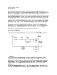
The dynamic system, shown in Figure 1-1, refers to the combination of the
control system and the plant.
Control System
Reference
Controller
Actuators
Physical System
(Plant)
Sensors
Figure 1-1. Dynamic System
The dynamic system in Figure 1-1 represents a closed-loop system, also
known as a feedback system. In closed-loop systems, the control system
monitors the outputs of the plant and adjusts the inputs to the plant to make
the actual response closer to the input that you designate.
One example of a closed-loop system is a system that regulates room
temperature. In this example, the reference input is the temperature at
which you want the room to stay. The thermometer senses the actual
temperature of the room. Based on the reference input, the thermostat
activates the heater or the air conditioner. In this example, the room is the
plant, the thermometer is the sensor, the thermostat is the controller, and the
heater or air conditioner is the actuator.
© National Instruments Corporation
1-1
Control Design User Manual
Chapter 1
Introduction to Control Design
Other common examples of control systems include the following
applications:
•
Automobile cruise control systems
•
Robots in manufacturing
•
Refrigerator temperature control systems
•
Hard drive head control systems
This chapter provides an overview of model-based control design and
describes how you can use the LabVIEW Control Design and Simulation
Module to design a controller.
Model-Based Control Design
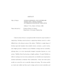
Model-based control design involves the following four phases:
developing and analyzing a model to describe a plant, designing and
analyzing a controller for the dynamic system, simulating the dynamic
system, and deploying the controller. Because model-based control design
involves many iterations, you might need to repeat one or more of these
phases before the design is complete. Figure 1-2 shows how National
Instruments provides solutions for each of these phases.
Plant Modeling
and Analysis
Control Design
and Simulation
Deployment
LabVIEW System
Identification
Toolkit
LabVIEW
Control Design and
Simulation Module
LabVIEW
Real-Time
Module
LabVIEW
Figure 1-2. Using LabVIEW in Model-Based Control Design
National Instruments also provides products for I/O and signal
conditioning that you can use to gather and process data. Using these tools,
which are built on the LabVIEW platform, you can experiment with
different approaches at each phase in model-based control design and
quickly identify the optimal design solution for a control system.
Control Design User Manual
1-2
ni.com
Chapter 1
Introduction to Control Design
Developing a Plant Model
The first phase of model-based control design involves developing and
analyzing a mathematical model of the plant you want to control. You can
use a process called system identification to obtain and analyze this model.
The system identification process involves acquiring data from a plant and
then numerically analyzing stimulus and response data to estimate the
parameters and order of the model.
The system identification process requires a combination of the following
components:
•
Signal generation and data acquisition—National Instruments
provides software and hardware that you can use to stimulate and
measure the response of the plant.
•
Mathematical tools to model a dynamic system—The LabVIEW
System Identification Toolkit contains VIs to help you estimate and
create accurate mathematical models of dynamic systems. You can use
this toolkit to create discrete linear models of systems based on
measured stimulus and response data.
This manual does not provide a comprehensive discussion of system identification.
Refer to the resources listed in the Related Documentation section of this manual for more
information about developing a plant model.
Note
Designing a Controller
The second phase of model-based control design involves two steps.
The first step is analyzing the plant model obtained during the system
identification process. The second step is designing a controller based on
that analysis. You can use the Control Design VIs and tools to complete
these steps. These VIs and tools use both classical and state-space
techniques.
Figure 1-3 shows the typical steps involved in designing a controller.
Determine
Specifications
Create
Mathematical
Model
Analyze
System
Synthesize
Controller
Figure 1-3. Control Design Process
© National Instruments Corporation
1-3
Control Design User Manual
Chapter 1
Introduction to Control Design
You often iterate these steps to achieve an acceptable design that is
physically realizable and meets specific performance criteria.
Simulating the Dynamic System
The third phase of model-based control design involves validating the
controller design obtained in the previous phase. You perform this
validation by simulating the dynamic system. For example, simulating a jet
engine saves time, labor, and money compared to building and testing an
actual jet engine.
You can use the Control Design and Simulation Module to simulate linear
time-invariant systems. This module also provides a variety of numerical
integration schemes for simulating more elaborate systems, such as
nonlinear systems. You also can use this module to determine how a system
responds to complex, time-varying inputs.
Deploying the Controller
The fourth phase of model-based control design involves deploying the
controller to a real-time (RT) target. LabVIEW and the LabVIEW
Real-Time Module provide a common platform that you can use to
implement the control system.
Refer to the National Instruments Web site at ni.com for information about
the National Instruments products mentioned in this section.
Overview of LabVIEW Control Design
The Control Design and Simulation Module provides an interactive
Control Design Assistant, a library of VIs, and a library of MathScript RT
Module functions for designing a controller based on a model of a plant.
You can use all these tools to complete the entire control design process
from creating a model of the controller to synthesizing the controller on an
RT target.
Control Design Assistant
You can use the Control Design Assistant to synthesize and analyze a
controller for a user-defined model without knowing how to program in
LabVIEW. You access the Control Design Assistant through the LabVIEW
SignalExpress environment. LabVIEW SignalExpress is a framework that
can host multiple interactive National Instruments tools and assistants.
Control Design User Manual
1-4
ni.com
Chapter 1
Introduction to Control Design
You also can use the Control Design Assistant to create a project. In one
project, you can load or create a model of a plant into the Control Design
Assistant, analyze the time or frequency response, and then calculate the
controller parameters. With the Control Design Assistant, you immediately
can see the mathematical equation and graphical representation that
describe the model. You also can view the response data and the
configuration of the controller.
Using the Control Design Assistant, you can convert a project to a
LabVIEW block diagram and customize that block diagram in LabVIEW.
You then can use LabVIEW to enhance and extend the capabilities of the
application. Refer to the LabVIEW SignalExpress Help for more
information about using the Control Design Assistant to analyze models
that describe a physical system and design controllers to achieve specified
dynamic characteristics.
Control Design VIs
The Control Design and Simulation Module also provides VIs that you can
use to create and develop control design applications in LabVIEW. You
can use these VIs to develop mathematical models of a dynamic system,
analyze the models to learn about their dynamic characteristics, and create
controllers to achieve specified dynamic characteristics. You use these VIs
to customize a LabVIEW block diagram to achieve specific goals. You also
can use other LabVIEW VIs and functions to enhance the functionality of
the application. Refer to the LabVIEW Help, available by selecting Help»
Search the LabVIEW Help, for information about the Control Design
VIs.
Unlike creating a project with the Control Design Assistant, creating a
LabVIEW application using the Control Design VIs requires basic
knowledge about programming in LabVIEW. Refer to the LabVIEW Help
for more information about the LabVIEW programming environment.
© National Instruments Corporation
1-5
Control Design User Manual
Chapter 1
Introduction to Control Design
Control Design MathScript RT Module Functions
The Control Design and Simulation Module also includes numerous
functions that extend the functionality of the LabVIEW MathScript
Window. Use these functions to design and analyze controller models in a
text-based environment. The LabVIEW MathScript Window is able to
process files you create using the current LabVIEW MathScript syntax and,
for backwards compatibility, files you created using legacy MathScript
syntaxes. The LabVIEW MathScript Window also can process certain of
your files that use other text-based syntaxes, such as files you created using
the MATLAB® software. Because the MathScript RT Module engine is
used to process scripts in the LabVIEW MathScript Window, and
because the MathScript RT Module engine does not support all syntaxes,
not all existing text-based scripts are supported.
Control Design User Manual
1-6
ni.com
Constructing Dynamic System
Models
2
Model-based control design relies upon the concept of a dynamic system
model. A dynamic system model is a mathematical representation of the
dynamics between the inputs and outputs of a dynamic system. You
generally represent dynamic system models with differential equations or
difference equations.
Obtaining a model of the dynamic system you want to control is the first
step in model-based control design. You analyze this model to anticipate
the outputs of the model when given a set of inputs. Using this analysis, you
then can design a controller that affects the outputs of the dynamic system
in a manner that you specify.
For example, consider the temperature-regulation example in the
introduction of Chapter 1, Introduction to Control Design. You can analyze
the open-loop dynamics of the plant to design an effective controller for this
closed-loop dynamic system. A model for this closed-loop dynamic system
describes the input to the plant as the air flow from the vent. The output of
the plant is the temperature of the room. By analyzing the relationship
between the inputs and output of the plant, you can predict how the plant
reacts when given certain inputs. Based on this analysis, you then can
design a controller for this dynamic system.
This chapter provides information about using the LabVIEW Control
Design and Simulation Module to create dynamic system models. This
chapter also describes the different forms that you can use to represent a
dynamic system model.
Note Refer to the labview\examples\Control and Simulation\Control
Design\Model Construction directory for example VIs that demonstrate the concepts
explained in this chapter.
© National Instruments Corporation
2-1
Control Design User Manual
Chapter 2
Constructing Dynamic System Models
Constructing Accurate Models
To create a model of a system, think of the system as a black box that
continuously accepts inputs and continuously generates outputs. Figure 2-1
shows the basic black-box model of a dynamic system.
Input
H(s)
Output
Figure 2-1. Black-Box Model of a Dynamic System
You refer to this model as a black-box model because you often do not
know the relationship between the inputs and outputs of a dynamic system.
The model you create, therefore, has errors that you must account for when
designing a controller.
An accurate model perfectly describes the dynamic system that it
represents. Real-world dynamic systems, however, are subject to a variety
of non-deterministic fluctuating conditions and interacting components
that prevent you from making a perfect model. You must consider many
external factors, such as random interactions and parameter variations. You
also must consider internal interacting structures and their fundamental
descriptions.
Because designing a perfectly accurate model is impossible, you must
design a controller that accounts for these inaccuracies. A robust controller
is one that functions as expected despite some differences between the
dynamic system and the model of the dynamic system. A controller that is
not robust might fail when such differences are present.
The more accurate a model is, the more complex the mathematical
relationship between inputs and outputs. At times, however, increasing the
complexity of the model does not provide any more benefits. For example,
if you want to control the interacting forces and friction of a mechanical
dynamic system, you might not need to include the thermodynamic effects
of the system. These effects are complicated features of the system that do
not affect the friction enough to impact the robustness of the controller.
A model that incorporates these effects can become unnecessarily
complicated.
Control Design User Manual
2-2
ni.com
Chapter 2
Constructing Dynamic System Models
Model Representation
You can represent a dynamic system using several types of dynamic system
models. You also can represent each type of dynamic system model using
three different forms. The following sections provide information about the
different types and forms of dynamic system models that you can construct
with the Control Design and Simulation Module.
Model Types
You base the type of dynamic system model on the properties of the
dynamic system that the model represents. The following sections provide
information about the different types of models you can create with the
Control Design and Simulation Module.
Linear versus Nonlinear Models
Dynamic system models are either linear or nonlinear. A linear model
obeys the principle of superposition. The following equations are true for
linear models.
y1 = ƒ(x1)
y2 = ƒ(x2)
Y = ƒ(x1 + x2) = y1 + y2
Conversely, nonlinear models do not obey the principle of superposition.
Nonlinear effects in real-world systems include saturation, dead-zone,
friction, backlash, and quantization effects; relays; switches; and rate
limiters. Many real-world systems are nonlinear, though you can linearize
the model to simplify a design or analysis procedure. You can use the
Trim & Linearize VIs to perform this linearization task.
The Control Design and Simulation Module supports both linear and
nonlinear models.
© National Instruments Corporation
2-3
Control Design User Manual
Chapter 2
Constructing Dynamic System Models
Time-Variant versus Time-Invariant Models
Dynamic system models are either time-variant or time-invariant. The
parameters of a time-variant model change with time. For example, you can
use a time-variant model to describe the mass of an automobile. As fuel
burns, the mass of the vehicle changes with time.
Conversely, the parameters of a time-invariant model do not change with
time. For an example of a time-invariant model, consider a simple robot.
Generally, the dynamic characteristics of robots do not change over short
periods of time.
The Control Design and Simulation Module supports time-invariant
models only.
Continuous versus Discrete Models
Dynamic system models are either continuous or discrete. Both continuous
and discrete system models can be linear or nonlinear and time-invariant or
time-variant. Continuous models describe how the behavior of a system
varies continuously with time, which means you can obtain the properties
of a system at any certain moment from the continuous model. Discrete
models describe the behavior of a system at separate time instants, which
means you cannot obtain the behavior of the system between any two
sampling points.
Continuous system models are analog. You derive continuous models of a
physical system from differential equations of the system. The coefficients
of continuous models have clear physical meanings. For example, you can
derive the continuous transfer function of a resistor-capacitor (RC) circuit
if you know the details of the circuit. The coefficients of the continuous
transfer function are the functions of R and C in the circuit. You use
continuous models if you need to match the coefficients of a model to some
physical components in the system.
Discrete system models are digital. You derive discrete models of a
physical system from difference equations or by converting continuous
models to discrete models. In computer-based applications, signals and
operations are digital. Therefore, you can use discrete models to implement
a digital controller or to simulate the behavior of a physical system at
discrete instants. You also can use discrete models in the accurate
model-based design of a discrete controller for a plant.
The Control Design and Simulation Module supports continuous and
discrete models.
Control Design User Manual
2-4
ni.com
Chapter 2
Constructing Dynamic System Models
Model Forms
You can use the Control Design and Simulation Module to represent
dynamic system models in the following three forms: transfer function,
zero-pole-gain, and state-space. Refer to the Constructing Transfer
Function Models section, the Constructing Zero-Pole-Gain Models
section, and the Constructing State-Space Models section of this chapter
for information about creating and manipulating these system models.
Table 2-1 shows the equations for the different forms of dynamic system
models.
Table 2-1. Definitions of Continuous and Discrete Systems
Model
Form
Continuous
Transfer
Function
Discrete
m–1
Zero-PoleGain
State-Space
m
m–1
m
b0 + b1 s + … + bm – 1 s
+ bm s
H ( s ) = --------------------------------------------------------------------------------------------n–1
n
a0 + a1 s + … + an – 1 s
+ an s
b0 + b1 z + … + bm – 1 z
+ bm z
H ( z ) = --------------------------------------------------------------------------------------------n–1
n
a0 + a1 z + … + an – 1 z
+ an z
H = Hi j
H = Hi j
k ( s – z1 ) ( s – z2 ) … ( s – zm )
H ( s ) = -----------------------------------------------------------------------------( s – p1 ) ( s – p2 ) … ( s – pn )
k ( z – z1 ) ( z – z2 ) … ( z – zm )
H ( z ) = -----------------------------------------------------------------------------( z – p1 ) ( z – p2 ) … ( z – pn )
H = Hi j
H = Hi j
x· = Ax + Bu
x ( k + 1 ) = Ax ( k ) + Bu ( k )
y = Cx + Du
y ( k ) = Cx ( k ) + Du ( k )
Continuous transfer function and zero-pole-gain models use the s variable to define
time, whereas discrete models in these forms use the z variable. Continuous state-space
models use the t variable to define time, whereas discrete state-space models use the
k variable.
Note
You can use these forms to describe single-input single-output (SISO),
single-input multiple-output (SIMO), multiple-input single-output
(MISO), and multiple-input multiple-output (MIMO) systems. The number
of sensors and actuators determines whether a dynamic system is a SISO,
SIMO, MISO, or MIMO system.
© National Instruments Corporation
2-5
Control Design User Manual
Chapter 2
Constructing Dynamic System Models
The following sections provide information about an example dynamic
system and how to represent this dynamic system using all three model
forms.
RLC Circuit Example
Figure 2-2 shows an example circuit consisting of a resistor R, an inductor
L, a current i(t), a capacitor C, a capacitor voltage vc(t), and an input
voltage vi(t).
L
vi (t )
i (t )
+
R
C
–
vc (t )
Figure 2-2. RLC Circuit
The following sections use this example to illustrate the creation of three
forms of dynamic system models.
Constructing Transfer Function Models
Transfer function models use polynomial functions to define the dynamic
relationship between inputs and outputs of a system. You analyze transfer
function models in the frequency domain. The following equations define
continuous and discrete transfer function models.
Continuous Transfer Function Model
m–1
m
m–1
m
b0 + b1 s + … + bm – 1 s
+ bm s
numerator ( s ) H ( s ) = ------------------------------------= --------------------------------------------------------------------------------n
–
1
n
denominator ( s )
+ an s
a0 + a1 s + … + an – 1 s
Discrete Transfer Function Model
b0 + b1 z + … + bm – 1 z
+ bm z
numerator ( z )
H ( z ) = -------------------------------------- = --------------------------------------------------------------------------------n
–
1
n
denominator ( z )
+ an z
a0 + a1 z + … + an – 1 z
Control Design User Manual
2-6
ni.com
Chapter 2
Constructing Dynamic System Models
Numerators of transfer function models describe the locations of the zeros
of the system. Denominators of transfer function models describe the
locations of the poles of the system.
Use the CD Construct Transfer Function Model VI to create continuous
SISO, SIMO, MISO, and MIMO system models in transfer function form.
This VI creates a data structure that defines the transfer function model and
contains additional information about the system, such as the sampling
time, input or output delays, and input and output names. Refer to the
Obtaining Model Information section of this chapter for information about
other properties of transfer function models.
SISO Transfer Function Models
Using the example in the RLC Circuit Example section of this chapter,
you can describe the voltage of the capacitor vc using the following
second order differential equation:
LCv··c + RCv· c + v c = v i
After taking the Laplace transform and rearranging terms, you then can
write the transfer function between the input voltage Vi and the capacitor
voltage Vc using the following equation.
1-----Vc ( s )
LC
------------- = ------------------------------- = H ( s )
2
1Vi ( s )
s + Rs
------ + -----L LC
You then can use H(s) to study the dynamic properties of the RLC circuit.
The following equation defines a continuous transfer function where
R = 20 Ω, L = 50 mH, and C = 10 μF.
6
2 × 10
H ( s ) = --------------------------------------------2
6
s + 400s + 2 × 10
© National Instruments Corporation
2-7
Control Design User Manual
Chapter 2
Constructing Dynamic System Models
Figure 2-3 shows how you use the CD Construct Transfer Function Model
VI to create this continuous transfer function model.
Figure 2-3. Creating a Continuous Transfer Function Model
The Numerator and Denominator inputs are arrays with zero-based
indexes. The ith element of the array corresponds to the ith order coefficient
of the polynomial. You define the coefficients in ascending order.
The CD Construct Transfer Function Model VI does not automatically cancel
polynomial roots appearing in both the numerator and the denominator of the transfer
function. Refer to Chapter 10, Model Order Reduction, for information about cancelling
pole-zero pairs.
Note
The CD Construct Transfer Function Model VI creates a continuous model.
You can create a discrete transfer function model in one of two ways. The
method you use depends on whether you know the coefficients of the
discrete transfer function model.
If you know the coefficients of the discrete transfer function model, you can
enter in the appropriate values for Numerator and Denominator and set
the Sampling Time (s) to a value greater than zero. Figure 2-4 shows this
process using a sampling time of 10 μs.
Figure 2-4. Using Coefficients to Create a Discrete Transfer Function Model
Control Design User Manual
2-8
ni.com
Chapter 2
Constructing Dynamic System Models
If you do not know the coefficients of the discrete transfer function model,
you must use the CD Convert Continuous to Discrete VI for the conversion.
Set the Sampling Time (s) parameter of this VI to a value greater than
zero. Figure 2-5 shows this process using a sampling time of 10 μs.
Figure 2-5. Using the CD Convert Continuous to Discrete VI to Create a Discrete
Transfer Function Model
Converting from a continuous model to a discrete model results in the
following equation:
–5
–5
9.9865 × 10 z + 9.9732 × 10
H ( z ) = --------------------------------------------------------------------------2
z – 1.9958z + 0.996
Refer to the Converting Continuous Models to Discrete Models section of
Chapter 3, Converting Models, for more information about converting
continuous models to discrete models.
SIMO, MISO, and MIMO Transfer Function Models
You can use the CD Construct Transfer Function Model VI to create
SIMO, MISO, and MIMO dynamic system models. This section uses a
MIMO dynamic system model as an example.
Consider the two-input two-output system shown in Figure 2-6.
© National Instruments Corporation
2-9
Control Design User Manual
Chapter 2
Constructing Dynamic System Models
MIMO System
U1
Y1
H11
H21
U2
H12
Y2
H22
Figure 2-6. MIMO System with Two Inputs and Two Outputs
You can define the transfer function of this MIMO system by using the
following transfer function matrix H, where each element represents a
SISO transfer function.
H =
H 11 H 12
H 21 H 22
Suppose the following equations define the SISO transfer functions
between each input-output pair.
1
H 11 = --s
2
H 12 = ----------s+1
s+3
H 21 = -------------------------2
s + 4s + 6
H 22 = 4
Select the MIMO instance of the CD Construct Transfer Function Model
VI to create a MIMO transfer function model. You then can specify each
transfer function between the j th input and the i th output as the ij th element
of the two-dimensional Transfer Function(s) input array. Figure 2-7
shows that the numerator-denominator pair of the first row and first column
corresponds to H11, the numerator-denominator pair of the first row and
second column corresponds to H12, and so on.
Control Design User Manual
2-10
ni.com
Chapter 2
Constructing Dynamic System Models
Figure 2-7. Creating a MIMO Transfer Function Model
The elements in the Numerator and Denominator arrays correspond to
the coefficients, in ascending order, of the numerator and denominator in
the Hij transfer function model. For example, the numerator of H11 is 1,
which corresponds to the zero-order coefficient. Therefore, the first
element in the Numerator array for H11 is 1. The denominator of H11 is s,
which means the value 0 corresponds to the zero-order coefficient and the
value 1 corresponds to the first-order coefficient. Therefore the first
element in the Denominator array for H11 is 0 and the second element is 1.
Symbolic Transfer Function Models
Symbolic models define the transfer function using variables rather than
numerical values. If you want to change the value of R, for example, you
only need to make the change in one location instead of several locations.
Select the SISO (Symbolic) or MIMO (Symbolic) instance of the
CD Construct Transfer Function Model VI to create a SISO or MIMO
symbolic transfer function model, respectively.
© National Instruments Corporation
2-11
Control Design User Manual
Chapter 2
Constructing Dynamic System Models
The following equation is a symbolic version of the transfer function
originally defined in the SISO Transfer Function Models section of this
chapter.
1
------LC
H ( s ) = ------------------------------2
Rs
1
s + ------ + ------L LC
Specify the Symbolic Numerator and Symbolic Denominator
coefficients using the variable names R, L, and C. You then specify values
of the numerator and denominator coefficients in the variables input,
as shown in Figure 2-8.
Figure 2-8. Creating a SISO Symbolic Transfer Function Model
Constructing Zero-Pole-Gain Models
Zero-pole-gain models are rewritten transfer function models. When you
factor the polynomial functions of a transfer function model, you get a
zero-pole-gain model. This factoring process shows the gain and the
locations of the poles and zeros of the system. The locations of these poles
determine the stability of the dynamic system.
You analyze zero-pole-gain models in the frequency domain. The
following equations define continuous and discrete zero-pole-gain models,
where the numerators and denominators are products of first-order
polynomials.
Control Design User Manual
2-12
ni.com
Chapter 2
Constructing Dynamic System Models
Continuous Zero-Pole-Gain Model
m
∏s + z
i
k ( s – z 1 ) ( s – z 2 )… ( s – z m )
i=0
- = --------------------------------------------------------------H i j ( s ) = k --------------------n
( s – p 1 ) ( s – p 2 )… ( s – p n )
s + pi
∏
i=0
Discrete Zero-Pole-Gain Model
m
∏z + z
i
k ( z – z 1 ) ( z – z 2 )… ( z – z m )
i=0
- = --------------------------------------------------------------H i j ( z ) = k --------------------n
( z – p 1 ) ( z – p 2 )… ( z – p n )
z + pi
∏
i=0
In these equations, k is a scalar quantity that represents the gain, zi
represents the locations of the zeros, and pi represents the locations of the
poles of the system model.
Numerators of zero-pole-gain models describe the location of the zeros of
the system. Denominators of zero-pole-gain models describe the location
of the poles of the system.
Use the CD Construct Zero-Pole-Gain Model VI to create SISO, SIMO,
MISO, and MIMO system models in zero-pole-gain form. This VI creates
a data structure that defines the zero-pole-gain model and contains
additional information about the system, such as the sampling time, input
or output delays, and input and output names. Refer to the Obtaining Model
Information section of this chapter for information about other properties
of zero-pole-gain models.
SISO Zero-Pole-Gain Models
Using the example in the RLC Circuit Example section of this chapter,
the following equation defines a continuous zero-pole-gain model where
R = 20 Ω, L = 50 mH, and C = 10 μF.
6
6
2 × 10
2 × 10
H ( s ) = ------------------------------------------------------------------------------------- = -----------------------------------------( s + 200 + 1400i ) ( s + 200 – 1400i )
( s + 200 ± 1400i )
© National Instruments Corporation
2-13
Control Design User Manual
Chapter 2
Constructing Dynamic System Models
This equation defines a model with one pair of complex conjugate poles at
–200 ± 1400i.
Figure 2-9 shows how you use the CD Construct Zero-Pole-Gain Model VI
to create this continuous zero-pole-gain model.
Figure 2-9. Creating a Continuous Zero-Pole-Gain Model
The CD Construct Zero-Pole-Gain Model VI creates a continuous model.
You create a discrete zero-pole-gain model in the same way you create a
discrete transfer function model. Refer to the SISO Transfer Function
Models section of this chapter for more information about creating a
discrete zero-pole-gain model.
SIMO, MISO, and MIMO Zero-Pole-Gain Models
You create SIMO, MISO, and MIMO zero-pole-gain models the same way
you create SIMO, MISO, and MIMO transfer function models. Refer to the
SIMO, MISO, and MIMO Transfer Function Models section of this chapter
for information about creating these forms of system models.
Symbolic Zero-Pole-Gain Models
You create symbolic zero-pole-gain models the same way you create
symbolic transfer function models. Refer to the Symbolic Transfer
Function Models section of this chapter for information about creating a
symbolic system model.
Constructing State-Space Models
Continuous state-space models use first-order differential equations to
describe the system. Discrete state-space models use difference equations
to describe the system. You analyze state-space models in the time domain.
Control Design User Manual
2-14
ni.com
Chapter 2
Constructing Dynamic System Models
Note State-space models can be either deterministic or stochastic. Deterministic models
do not account for noise, whereas stochastic models do. This chapter provides information
about deterministic state-space models. Refer to Chapter 16, Using Stochastic System
Models, for information about stochastic state-space models.
The following equations define a continuous and a discrete state-space
model.
Continuous State-Space Model
x· = Ax + Bu
y = Cx + Du
Discrete State-Space Model
x ( k + 1 ) = Ax ( k ) + Bu ( k )
y ( k ) = Cx ( k ) + Du ( k )
Table 2-2 describes the dimensions of the vectors and matrices of a
state-space model.
Table 2-2. Dimensions and Names of State-Space Model Variables
© National Instruments Corporation
Variable
Dimension
k
—
Discrete time
n
—
Number of states
m
—
Number of inputs
r
—
Number of outputs
A
n × n matrix
State matrix
B
n × m matrix
Input matrix
C
r × n matrix
Output matrix
D
r × m matrix
Direct transmission matrix
x
n-vector
State vector
u
m-vector
Input vector
y
r-vector
Output vector
2-15
Name
Control Design User Manual
Chapter 2
Constructing Dynamic System Models
Use the CD Construct State-Space Model VI to create SISO, SIMO, MISO,
and MIMO system models in state-space form. This VI creates a data
structure that uses matrices to define the state-space model. The matrices
are zero-based two-dimensional arrays of numbers where the ij th element of
the array corresponds to the ij th element of matrices in a state-space model.
You can assume that an nth order system with m inputs and r outputs has
state, input, and output vectors as defined in the following equations:
x0
x =
u0
x1
..
.
u1
..
u =
xn – 1
y0
y =
um – 1
y1
..
yr – 1
State-space models also contain additional information about the system,
such as the sampling time, input or output delays, and input and output
names. Refer to the Obtaining Model Information section of this chapter for
information about other properties that state-space models contain.
SISO State-Space Models
Using the example in the RLC Circuit Example section of this chapter,
the following equations define a continuous state-space model.
·
0 1 v
0
v
c
x· = c =
+
1- –R
1 - vi
··
– -------- v·
-----vc
c
LC L
LC
y = vc = 1 0
vc
+ 0 vi
·
vc
In these equations, y equals the voltage of the capacitor vc, and u equals the
input voltage vi.
vc
x equals the voltage of the capacitor and the derivative of that voltage
.
·
vc
Control Design User Manual
2-16
ni.com
Chapter 2
Constructing Dynamic System Models
The following matrices define a state-space model where R = 20 Ω,
L = 50 mH, and C = 10 μF.
A =
0
1
6
– 2 × 10 – 400
B =
0
2 × 10
6
C = 1 0 D = 0
When you plug these matrices into the equations for a continuous
state-space model defined in the Constructing State-Space Models section
of this chapter, you get the following equations:
x· =
vc
0
+
v
·
6 i
– 2 × 10 – 400 v c
2 × 10
0
1
6
y = 10
vc
+ 0 vi
·
vc
Figure 2-10 shows how you use the CD Construct State-Space Model VI to
create this continuous state-space model.
Figure 2-10. Creating a Continuous State-Space Model
Although B is a column vector, C is a row vector, and D is a scalar, you must use the
2D array data type when connecting these inputs to the VI.
Note
© National Instruments Corporation
2-17
Control Design User Manual
Chapter 2
Constructing Dynamic System Models
The CD Construct State-Space Model VI creates a continuous model. You
create a discrete state-space model in the same way you create a discrete
transfer function model. Refer to the SISO Transfer Function Models
section of this chapter for more information about creating a discrete
state-space model.
SIMO, MISO, and MIMO State-Space Models
You construct a SIMO, MISO, or MIMO state-space model by ensuring the
output matrix C and the input matrix B have the appropriate dimensions.
For a SIMO system, construct an output matrix C with more than one row.
For a MISO system, construct an input matrix B with more than one
column. For a MIMO system, construct matrices C and B with more than
one row and column, respectively.
When you create a SIMO, MISO, or MIMO system, ensure that the direct
transmission matrix D has the appropriate dimensions. If you leave D
empty or unwired, the Control Design and Simulation Module replaces the
missing values with zeros.
Symbolic State-Space Models
You create symbolic state-space models the same way you create a
symbolic transfer function model. Refer to the Symbolic Transfer Function
Models section of this chapter for more information about creating a
symbolic system model.
Obtaining Model Information
Each of the Model Construction VIs creates not only a data structure that
defines the model, but also a set of properties that provide information
about the system. These properties are common in all three model forms.
Table 2-3 lists the properties and their corresponding data types.
Table 2-3. Model Properties
Property
Data Type
Description
Model Name
String
Assigns a name to a specific model.
Input Names
1D array of strings
The i th element of the array defines the
name of the i th input to the model.
Output Names
1D array of strings
The i th element of the array defines the
name of the i th output of the model.
Control Design User Manual
2-18
ni.com
Chapter 2
Constructing Dynamic System Models
Table 2-3. Model Properties (Continued)
Property
Data Type
Description
Input Delays
1D array of double-precision,
floating-point numeric values
The i th element of the array defines the time
delay of the i th input of the model.
Output Delays
1D array of double-precision,
floating-point numeric values
The i th element of the array defines the time
delay of the i th output of the model.
Transport Delay
1D array of double-precision,
floating-point numeric values
The ij th element of the array defines the time
delay between the i th output and j th input of
the model.
Notes
String
A string for storing additional data. The
string can contain comments or other
information that you want to store with the
model.
Sampling Time
Double-precision,
floating-point numeric value
Represents the sampling time, in seconds,
of the system. If a model represents a
continuous system, the value of Sampling
Time is zero. For discrete system models,
the value must be greater than zero.
State Names
Array of strings
The i th element of the array defines the
name of the i th state of the model. This
property is available with state-space
models only.
You can use these data structures with every VI in the Control Design and
Simulation Module that accepts a system model as an input.
Delay information exists in the model properties and not in the mathematical model.
Any analysis, such as time- or frequency-domain analysis, you perform on the model does
not account for delay present in the model. If you want the analysis to account for delay
present in the model, you must incorporate the delay into the model itself. Refer to
Chapter 6, Working with Delay Information, for more information about accounting for
model delay.
Note
You can use the Model Information VIs to get and set various properties
of the model. Refer to the LabVIEW Help, available by selecting Help»
Search the LabVIEW Help, for more information about using the Model
Information VIs to view and change the properties of a system model.
© National Instruments Corporation
2-19
Control Design User Manual
3
Converting Models
Model conversion involves changing the representation of dynamic system
models. For example, you can convert a zero-pole-gain model to a
state-space model. You also can convert a model between continuous and
discrete types.
This chapter provides information about using the LabVIEW Control
Design and Simulation Module to convert between model forms and to
convert between continuous and discrete models.
Note Refer to the labview\examples\Control and Simulation\Control
Design\Model Conversion directory for example VIs that demonstrate the concepts
explained in this chapter.
Converting between Model Forms
You can use three different model forms—transfer function,
zero-pole-gain, and state-space—to describe the same dynamic system.
Refer to Chapter 2, Constructing Dynamic System Models, for more
information about these model forms. You can use the Control Design and
Simulation Module to convert from one form to another.
Converting between model forms is important because each form provides
different information about the system. For example, state-space models
use the states of a system to show physical information about the system.
Thus, observing physical information about a dynamic system is less
complicated when the model for that dynamic system is in state-space
form.
You also can use different analysis and synthesis techniques depending on
the form of the model. For example, if a model for a system is in transfer
function form, you can synthesize a controller for that system using
classical control design techniques such as the root locus technique. If the
model is in state-space form, you can design a controller using state-space
control design techniques such as the pole placement technique. Refer to
Chapter 11, Designing Classical Controllers, and Chapter 12, Designing
State-Space Controllers, for more information about classical and
state-space control design techniques.
© National Instruments Corporation
3-1
Control Design User Manual
Chapter 3
Converting Models
The following sections discuss the Model Conversion VIs you can use to
convert between model forms.
Converting Models to Transfer Function Models
Use the CD Convert to Transfer Function Model VI to convert a
zero-pole-gain or state-space model to a transfer function model. This
section uses a state-space model as an example.
Note Because transfer function models do not include state information, you lose the state
vector x when you convert a state-space model to a transfer function model. Additionally,
the Control Design and Simulation Module might not be able to recover the same states if
you convert the model back to state-space form.
Consider the continuous state-space model defined in the Constructing
State-Space Models section of Chapter 2, Constructing Dynamic System
Models.
x· = Ax + Bu
y = Cx + Du
For continuous systems, you can use the Laplace transform to convert from
the time domain to the Laplace domain model representation.
The equations in this section convert model forms within both the continuous and
discrete domains. Refer to the Converting between Continuous and Discrete Models
section of this chapter for information about converting between continuous and discrete
domains.
Note
Applying the Laplace transform to the state-space model results in the
following equation:
–1
Y ( s ) = [ C ( Is – A ) B + D ]U ( s )
In this equation, s is the Laplace variable, and I is the identity matrix with
the same dimensions as A.
Control Design User Manual
3-2
ni.com
Chapter 3
Converting Models
The ratio between the output Y(s) and input U(s) defines the following
matrix transfer function model H(s).
Y(s)
–1
H ( s ) ≡ ----------- = C ( Is – A ) B + D
U(s)
For example, consider the following second-order MISO state-space
system model.
x· = – 1 2 x + 1 0 u
0 –1
0 1
y = 1 0 x+ 0 0 u
Using the Laplace transform, you obtain the transfer function matrix H(s).
1
2
H ( s ) = ----------- ------------------------s + 1 s 2 + 2s + 1
Converting Models to Zero-Pole-Gain Models
Use the CD Convert to Zero-Pole-Gain Model VI to convert a transfer
function or state-space model to a zero-pole-gain model. This section uses
a transfer function model as an example.
When you convert a state-space model to a zero-pole-gain model, the CD Convert
to Zero-Pole-Gain Model VI converts the state-space model to a transfer function model
first.
Note
To convert the transfer function matrix H(s) to the zero-pole-gain form,
the Control Design and Simulation Module calculates the numerator and
denominator polynomial roots and the gain of each SISO transfer function
in H(s).
© National Instruments Corporation
3-3
Control Design User Manual
Chapter 3
Converting Models
When you convert the transfer function matrix from the Converting Models
to Transfer Function Models section of this chapter, you obtain the
following zero-pole-gain model:
1
2
H ( s ) = ----------- ------------------2
s + 1 (s + 1)
This zero-pole-gain model is numerically identical to the transfer function
model. The zero-pole-gain form, however, shows the locations of the zeros
and poles of a system.
Converting Models to State-Space Models
Use the CD Convert to State-Space Model VI to convert a zero-pole-gain
or transfer function model to a state-space model. This section uses a
zero-pole-gain model as an example.
When you convert a zero-pole-gain model to a state-space model, the CD Convert
to State-Space Model VI converts the zero-pole-gain model to a transfer function model
first.
Note
When converting a transfer function or zero-pole-gain model, you can
specify whether you want the resulting state-space model to be full or
minimal. A full state-space model does not reduce the number of states
determined by a least common denominator calculation. A minimal
state-space model reduces the number of states and produces a minimal
representation of the original model. Use the Realization Type parameter
of the CD Convert to State-Space Model VI to specify if you want the
resulting model to be full or minimal. Refer to the Obtaining the Minimal
Realization of Models section of Chapter 10, Model Order Reduction,
for more information about minimizing state-space realizations.
Using the example in the Converting Models to Transfer Function Models
section of this chapter, the following equation gives the minimal realization
when converting a zero-pole-gain model to a state-space model.
x· = – 0.33 0.94 x + – 0.41 0 u
– 0.47 – 1.67
0.29 – 0.87
y = – 2.45 0 x + 0 0 u
Control Design User Manual
3-4
ni.com
Chapter 3
Converting Models
This model numerically differs from the initial state-space model. From the
input-output model perspective, however, the state-space models are
identical.
Refer to the LabVIEW Help, available by selecting Help»Search the
LabVIEW Help, for more information about the Model Conversion VIs.
Converting between Continuous and Discrete Models
Continuous models are analog and operate using physical components.
Discrete models are digital and operate on a computer or real-time (RT)
target. To determine how an analog model performs on a digital target, you
can convert the continuous model to a discrete model. You also can convert
a discrete model to a continuous model.
Additionally, you can resample a discrete model. Resampling involves
converting a discrete model to a discrete model with a different sampling
time. Resampling is useful when the sampling time of a model does not
match the sampling time of the target on which that model operates. In this
situation, you resample the model to use the sampling time of the target.
The Model Conversion VIs provide a number of mathematical methods that
perform these conversions. Table 3-1 summarizes these methods, which are
substitutions between the continuous Laplace-transform operator and the
discrete z-transform operator.
Table 3-1. Mapping Methods for Converting between Continuous and Discrete
Method of Approximation
Continuous to Discrete
Discrete to Continuous
Forward Rectangular
Method
z–1
s → ----------T
z → 1 + sT
Backward Rectangular
Method
z–1
s → ----------zT
1
z → --------------1 – sT
© National Instruments Corporation
3-5
Control Design User Manual
Chapter 3
Converting Models
Table 3-1. Mapping Methods for Converting between Continuous and Discrete (Continued)
Method of Approximation
Continuous to Discrete
Discrete to Continuous
Tustin’s Method
2(z – 1)
s → -------------------T(z + 1)
sT
1 + -----2
z → --------------sT
1 – -----2
Prewarp Method
z(z – 1)
s → ----------------------T ∗(z + 1)
1 + sT ∗
z → ------------------1 – sT ∗
w×T
2 tan ------------- 
 2 
T ∗ = ------------------------------w
w×T
2 tan ------------- 
 2 
T ∗ = ------------------------------w
In these equations, T represents the sample time and w represents the
prewarp frequency. T* is a modified sample time that the Prewarp method
uses in converting between continuous and discrete models.
The following sections provide information about the methods that you can
use to perform continuous to discrete conversions, discrete to continuous
conversions, and discrete to discrete conversions.
Converting Continuous Models to Discrete Models
To convert a continuous model to a discrete one, first approximate the
value of the derivative in the continuous equation over each change in time.
Then find the area of the geometric region having width dt and height equal
to the derivative.
For example, consider the following first-order continuous differential
equation:
y· = f ( t )
Control Design User Manual
3-6
ni.com
Chapter 3
Converting Models
To convert this continuous model to a discrete model, evaluate the
derivative function ƒ(t) at different points to approximate y· at time t.
Figure 3-1 illustrates the function ƒ(t) between t and t + T, where T is the
sampling time.
f(t)
t
t+T
Figure 3-1. Discretizing a Differential Equation
Integrating between time t and t + T results in the following difference
equation:
t+T
t+T
 y· d τ = y ( t + T ) – y ( t ) =  f ( τ ) d τ
t
t
Integrating f(τ) for τ = t to t + T represents the area under the curve.
The CD Convert Continuous to Discrete VI provides the following
mathematical methods to approximate this area.
•
Forward Rectangular
•
Backward Rectangular
•
Tustin’s
•
Prewarp
•
Zero-Order-Hold
•
First-Order-Hold
•
Z-Transform
•
Matched Pole-Zero
The following sections provide information about each of these methods.
© National Instruments Corporation
3-7
Control Design User Manual
Chapter 3
Converting Models
Forward Rectangular Method
The Forward Rectangular method considers ƒ(τ) constant and equal to ƒ(t)
along the integration range. This consideration results in the following
equation:
y ( t + T ) = y ( t ) + f ( t )T
This method considers the incremental area term between sampling times t
and t + T as a rectangle of width T and height equal to ƒ(t), as shown in
Figure 3-2.
Forward
f(t + T)
f(t)
t
t+T
Figure 3-2. Forward Rectangular Method
Figure 3-2 shows that, for this example, the Forward Rectangular method
underestimates the area under the curve. To minimize this underestimation,
use a small sampling interval. Depending on the direction and size of the
curve you are measuring, this underestimation might not occur.
Backward Rectangular Method
The Backward Rectangular method considers ƒ(τ) constant and equal to
ƒ(t + T) along the integration range. This consideration results in the
following equation:
y ( t + T ) = y ( t ) + f ( t + T )T
Control Design User Manual
3-8
ni.com
Chapter 3
Converting Models
This method considers the incremental area term between sampling times t
and t + T as a rectangle of width T and height equal to ƒ(t + T ), as shown
in Figure 3-3.
Backward
f(t + T)
f(t)
t
t+T
Figure 3-3. Backward Rectangular Method
Figure 3-3 shows that, for this example, the Backward Rectangular method
overestimates the area under the curve. To minimize this overestimation,
use a small sampling interval. Depending on the direction and size of the
curve you are measuring, this overestimation might not occur.
Tustin’s Method
Tustin’s method, also known as the trapezoid method, uses trapezoids
to provide a balance between the Forward Rectangular and Backward
Rectangular methods. Tustin’s method takes the average of the rectangles
defined by the Forward and Backward Rectangular methods and uses the
average value as the incremental area to approximate the area under the
curve.
Tustin’s method considers ƒ(τ) constant and equal to the average between
ƒ(t) and ƒ(t + T) along the integration range, which results in the following
equation:
[ f (t) + f (t + T )]
y ( t + T ) = y ( t ) + ----------------------------------------- T
2
© National Instruments Corporation
3-9
Control Design User Manual
Chapter 3
Converting Models
The last term in this equation is identical to the area of a trapezoid of height
T and bases ƒ(t) and ƒ(t + T). Figure 3-4 shows the area under a curve using
Tustin’s method.
Tustin
t
t+T
Figure 3-4. Tustin’s Method
Figure 3-4 shows that, for this example, Tustin’s method provides a balance
between the underestimation of the Forward Rectangular and the
overestimation of the Backward Rectangular method.
Prewarp Method
The Prewarp method is a trapezoidal type of transformation that uses the
prewarp frequency ω to adjust the sampling time T. This adjustment results
in a separate sampling time T *. This adjustment also compensates for errors
introduced in the discretizing process.
This method also considers ƒ(τ) constant and equal to the average between
ƒ(t) and ƒ(t + T * ) along the integration range, which results in the
following equation:
[ f (t) + f (t + T *)]
y ( t + T ) = y ( t ) + ------------------------------------------- T
2
Control Design User Manual
3-10
ni.com
Chapter 3
Converting Models
The last term in this equation is identical to the area of a trapezoid of
height T and bases ƒ(t) and ƒ(t + T *). Figure 3-5 shows the area under a
curve using the Prewarp method.
Prewarp
t
t + T t + T*
Figure 3-5. Prewarp Method
Figure 3-5 shows that, for this example, the Prewarp method compensates
for the integration error by adjusting the sampling time to T*. The area
between t + T and t + T* is roughly equal to the integration error, which is
represented by the unshaded portion of the area under the curve.
Use a particular conversion method based on the model that you are
converting and the requirements of the application for which you are
designing a control system.
Zero-Order-Hold and First-Order-Hold Methods
The Zero-Order-Hold and First-Order-Hold methods assume properties of
the continuous differential equation y· = f ( t ) . The Zero-Order-Hold
method assumes that ƒ(t) consists of an input that you can hold constant
during the integration period between sampling times t and t + T. The
First-Order-Hold method assumes that you can increase this input over
time during this same period. These methods also integrate the remaining
terms of ƒ(t) not related to the input because these terms refer to the internal
state dynamics.
© National Instruments Corporation
3-11
Control Design User Manual
Chapter 3
Converting Models
You obtain the following equation after integrating a linear time-invariant
system between sampling times t and t + T.
t+T
x(t + T ) = e
AT
x(t) +
e
A(t + T + τ)
Bu ( τ )d τ
t
y ( t ) = Cx ( t ) + Du ( t )
In this equation, u(t) is the input to the system and is not necessarily
constant between sampling times t and t + T. The following equation shows
the Zero-Order-Hold method approximating the input to a constant value
u(t) during the integration time.
t+T
x(t + T ) = e
AT
x(t) +
e
A(t + T + τ)
Bd τ u ( t )
t
Conversely, the following equation shows the First-Order-Hold method
ramping the input values with a constant slope [u(t + T) – u(t)]/T during
integration time.
t+T
x(t + T ) = e
AT
x(t) +
e
A(t + T + τ)
t

(τ – t) 
B  u ( t ) + [ u ( t + T ) – u ( t ) ] --------------- d τ
T 

Refer to Digital Control of Dynamic Systems, as listed in the Related
Documentation section of this manual, for more information about the
Zero-Order-Hold and First-Order-Hold methods.
Z-Transform Method
The Z-Transform method is defined such that the continuous and discrete
impulse responses maintain major similarities. You calculate the impulse
response of the discrete transfer function by multiplying the inverse
Laplace transform of the continuous transfer function by the sampling
time T.
Refer to Discrete-Time Control Systems, as listed in the Related
Documentation section of this manual, for more information about the
Z-Transform method.
Control Design User Manual
3-12
ni.com
Chapter 3
Converting Models
Matched Pole-Zero Method
The Matched Pole-Zero method uses the following relationship between
the continuous s and discrete z frequency domains.
z = e
sT
In this equation, T is the sampling time used for the discrete system. The
Matched Pole-Zero method maps continuous-time poles and finite zeros to
the z-plane using this relation. This method also maps zeros at infinity to
z = 0, so these zeros do not affect the frequency response.
After the algorithm maps the poles and zeros, the algorithm then attempts
to make sure the system gains are equivalent at some critical frequency. If
the systems have no poles or zeros at s = 0 or z = 1, the Matched Pole-Zero
method selects a discrete-time gain such that the system gains match at
these locations.
Alternatively, if the systems have no poles or zeros at s = p(i/T) or z = –1,
where p is the location of a pole, this method equalizes the gains at that
frequency. If the Matched Pole-Zero method cannot match either of these
gains, the algorithm does not choose a gain.
Refer to Digital Control of Dynamic Systems, as listed in the Related
Documentation section of this manual, for more information about the
Matched Pole-Zero method.
Converting Discrete Models to Continuous Models
Use the CD Convert Discrete to Continuous VI to convert a discrete model
to a continuous model. This VI supports the following conversion methods:
Forward Rectangular, Backward Rectangular, Tustin’s, Prewarp,
Z-Transform, and Zero-Order-Hold. This VI does not support the
First-Order-Hold or Matched Pole-Zero methods. Refer to Table 3-1 for
the equations for each mapping method.
The Z-Transform method also is a reverse calculation to map a model in the
z-plane to the s-plane. You calculate the impulse response of the continuous
transfer function by dividing the inverse z-transform of the discrete transfer
function by the sampling time T.
© National Instruments Corporation
3-13
Control Design User Manual
Chapter 3
Converting Models
Resampling a Discrete Model
Use the CD Convert Discrete to Discrete VI to resample a discrete model.
This VI converts the discrete model to a continuous model and then
converts the continuous model back to a discrete model. The first
conversion uses the initial sampling time T1. The second conversion uses
the final sampling time T2.
The CD Convert Discrete to Discrete VI supports the following conversion
methods: Forward Rectangular, Backward Rectangular, Tustin’s, Prewarp,
Zero-Order-Hold, and Z-Transform. This VI does not support the
First-Order-Hold or Matched Pole-Zero methods.
Control Design User Manual
3-14
ni.com
4
Connecting Models
You typically create a dynamic system model by connecting many models,
or subsystems, together. Connecting many models together makes
developing a model of a complicated dynamic system less complicated
because you can describe the dynamics of individual pieces.
You can connect continuous models only to other continuous models. To
connect discrete models together, each model must have the same sampling
time. Connected models might, however, be of any form. For example,
you can connect a transfer function model to a state-space model or a
state-space model to a zero-pole-gain model.
Furthermore, you can make connections between single-input
single-output (SISO), single-input multiple-output (SIMO), multiple-input
single-output (MISO), and multiple-input multiple-output (MIMO)
systems.
This chapter provides information about using the LabVIEW Control
Design and Simulation Module to connect models in the following four
ways: in series, by appending, in parallel, and with feedback.
Note Refer to the labview\examples\Control and Simulation\Control
Design\Model Connection directory for example VIs that demonstrate the concepts
explained in this chapter.
Connecting Models in Series
A series connection joins the outputs of the first model to the inputs of a
second model. Use the CD Series VI to connect two models in series.
Note When connecting models of different forms, the Series Model output returns a
model based on the following hierarchy: state-space>transfer function>zero-pole-gain.
For example, if you connect a zero-pole-gain model to a state-space model, Series Model
returns a state-space model.
The following sections provide information about the kinds of connections
you can make with the CD Series VI.
© National Instruments Corporation
4-1
Control Design User Manual
Chapter 4
Connecting Models
Connecting SISO Systems in Series
Consider a valve that controls the flow rate of water into a tank. Figure 4-1
represents this system.
I(s): Input Signal
Q(s): Flow Rate
Hv(s)
Ht (s)
L
L(s): Level
Figure 4-1. Flow of Water into a Tank
If you assume that the incoming water pressure to the valve is constant,
only the valve input signal affects the level of the water in the tank. You can
model the flow rate of water into the tank using the following transfer
functions, where Hv(s) is a model of the valve and Ht(s) is a model of the
tank.
Kv
Q(s)
H v ( s ) ≡ ----------- = -----------------------------------2 2
I(s)
τ s + 2ζτs + 1
K
L(s)
H t ( s ) ≡ ----------- = -----t
Q(s)
s
I(s), Q(s), and L(s) represent the Laplace transform of the input signal, the
flow rate, and the level of water in the tank, respectively. The constants Kv,
τ, ζ, and Kt are parameters of the models that describe the valve and tank.
To obtain the effect of the input signal on the water level, place the two
systems in series and multiply their transfer functions.
K
Kv
L(s)
- ⋅ -----t
H ( s ) ≡ ---------- = H v ( s ) ⋅ H t ( s ) = -----------------------------------2 2
I(s)
τ s + 2ζτs + 1 s
Control Design User Manual
4-2
ni.com
Chapter 4
Connecting Models
This equation represents the output of Hv(s) connecting to the input of
Ht(s). Figure 4-2 illustrates this relationship.
I(s)
Hv(s) = Q(s)/I(s)
I(s)
Q(s)
Ht(s) = L(s)/Q(s)
H(s) = Hv(s)*Ht (s) = L(s)/I(s)
L(s)
L(s)
Figure 4-2. Valve Model and Tank Model in Series
The resulting SISO system H(s) now represents the relationship between
the input signal I(s) and the level of water L(s) in the tank.
Creating a SIMO System in Series
You can create a SIMO system by connecting two or more SISO systems
with a SIMO subsystem. For example, adding another valve and tank to the
example in the Connecting SISO Systems in Series section of this chapter
results in a SIMO system that divides the flow rate between two different
tanks. Figure 4-3 shows this system.
I(s): Input Signal
Q(s): Flow Rate
Hv 1(s)
Q1(s)
Q2(s)
Hv 2(s)
Ht 1(s)
L1(s): Level Tank 1
L1
Ht 2(s)
L2
L2(s): Level Tank 2
Figure 4-3. Dividing the Flow of Water between Two Tanks
© National Instruments Corporation
4-3
Control Design User Manual
Chapter 4
Connecting Models
Hv2(s) is a SIMO transfer function matrix that represents the relationship of
the flow rates. By connecting Hv2(s) to Hv1(s) and Q(s), the entire system
becomes SIMO. The total flow rate Q(s) is equal to the sum of the parts
Q1(s) and Q2(s).
Q ( s ) = Q 1 ( s ) + Q 2 ( s ) = λQ ( s ) + ( 1 – λ )Q ( s )
The constant λ represents the fraction of flow sent to the first tank, whereas
(1 – λ) is the remaining fraction of flow sent to the second tank.
H v2 ( s ) =
λ
1–λ
When you connect these models in series, the output of the first system
Hv1(s) connects to the input of the second system Hv2(s). Figure 4-4
illustrates this relationship.
Q1(s) = λQ (s)
I (s)
Hv1(s) = Q(s)/I(s)
Q(s)
Hv 2(s)
Q2(s) = (1 – λ)Q(s)
Ht 1(s) = L1(s)/Q1(s)
Ht 2(s) = L2(s)/Q2(s)
L1(s)
L2(s)
Figure 4-4. Two Valve Models and Two Tank Models in Series
This combined system, which now is a SIMO system, has one input I(s) and
two outputs L1(s) and L2(s). Figure 4-5 is a LabVIEW block diagram that
illustrates this system.
Figure 4-5. Block Diagram of the Two Valves and Tanks in Series
Control Design User Manual
4-4
ni.com
Chapter 4
Connecting Models
Connecting MIMO Systems in Series
When connecting MIMO systems, you can connect any output of the first
model to any input(s) of the second model. Figure 4-6 shows an example
of two MIMO system models connected in series.
u0
z0
u1
z1
u2
Model 1
uj
z1
z2
zl
zl
v0
y0
v1
y1
v2
vk
Model 2
y2
yi
Figure 4-6. MIMO System Models in Series
Figure 4-6 shows how the outputs of Model 1 that are connected to the
inputs of Model 2 do not appear as outputs of the resulting series model.
For example, because z0 connects to the Model 2 inputs v1 and v2, z0 is no
longer an output of the resulting series model. Similarly, because z2
connects to v0, z2 is no longer an output of the resulting series model.
© National Instruments Corporation
4-5
Control Design User Manual
Chapter 4
Connecting Models
This same principle applies to the inputs of Model 2. Inputs of Model 2 that
are connected to an output of Model 1 no longer appear as inputs of the
resulting series model. Because the input v0 of Model 2 is connected to the
output of z2 of Model 1, neither v0 nor z2 appear in the resulting series
model.
You define the connections between two models using the Connections
control of the CD Series VI. Figure 4-7 shows the settings this control used
to connect the models in Figure 4-6.
Figure 4-7. Connection Definitions for Models in Series
The control in Figure 4-7 indicates that the Model 1 output z0 connects to
the Model 2 inputs v1 and v2. You also can see how the Model 1 output z2
connects to the Model 2 input v0.
Appending Models
You can append models together to compare the time or frequency
response of two models in the same plot. Use the CD Append VI to produce
an augmented model from connections between two models. This
augmented model contains all inputs and outputs of both models. With
state-space models, states of the first model are combined with states of the
second model.
Control Design User Manual
4-6
ni.com
Chapter 4
Connecting Models
Figure 4-8 shows two appended system models.
u0
z0
u1
z1
u2
z2
Model 1
uj
zl
v0
y0
v1
y1
v2
y2
Model 2
vk
yi
Figure 4-8. Appended Models
For example, consider the two tanks from the Creating a SIMO System in
Series section of this chapter. The following equations define the transfer
functions of the tanks.
K
H t1(s) = -----1s
K
H t2(s) = -----2s
K1 and K2 are the gains of their respective transfer functions. Appending
Ht1(s) and Ht2(s) results in the following appended matrix transfer
function Ht.
Ht =
© National Instruments Corporation
4-7
H t1 ( s )
0
0
H t2 ( s )
Control Design User Manual
Chapter 4
Connecting Models
Figure 4-9 uses the block diagram from Figure 4-5 but replaces the Tanks
input with Ht. As in Figure 4-5, the two valves are connected in series with
each other. In Figure 4-9, however, the two tanks now are appended to each
other.
Figure 4-9. Appending the Two Tanks
Connecting Models in Parallel
A parallel connection creates a single model from two separate systems that
share common inputs. You also can use a parallel connection to add or
subtract outputs of two subsystems and represent them as a single output.
Use the CD Parallel VI to connect systems in parallel.
For example, consider the circuit system in Figure 4-10.
i
i1
R1
i2
R2
v
L1
L2
Figure 4-10. Circuit System
Control Design User Manual
4-8
ni.com
Chapter 4
Connecting Models
The input of this system is the voltage v. The output of this system is the
total current i, which is the sum of currents i1 and i2. R1 and R2 are resistors,
and L1 and L2 are inductors. The following equations describe the
individual currents for the circuit system in Figure 4-10.
di
L 1 ------1- + R 1 i 1 – v = 0
dt
di 2
L 2 ------- + R 2 i 2 – v = 0
dt
The following equations give the resulting transfer functions for each
circuit loop.
I1 ( s )
1
= -------------------H 1 ( s ) = ----------L1 s + R1
V(s)
I2 ( s )
1
H 2 ( s ) = ----------= -------------------V(s)
L2 s + R2
In Figure 4-11, H1(s) and H2(s) represent the transfer functions defined in
the previous equations, and I1(s) and I2(s) are the respective outputs of these
transfer functions. V(s) is the transfer function of the voltage input v that
both circuit loops share.
V(s)
H1(s)
I1(s)
V(s)
H2(s)
I2(s)
Figure 4-11. Each Circuit Loop in the Circuit System
© National Instruments Corporation
4-9
Control Design User Manual
Chapter 4
Connecting Models
Figure 4-12 illustrates the relationship between the voltage input v and total
current i by placing both models together in one larger system model. When
the two models are in parallel, both models share the same input V(s) and
provide a total output I(s), as shown in Figure 4-12.
H1(s)
V(s)
I(s)
H2(s)
Figure 4-12. Entire Circuit System as a Parallel Model
The following equations describe the resulting transfer function as a
second-order system.
I ( s ) = I1 ( s ) + I2 ( s ) = V ( s ) [ H1 ( s ) + H2 ( s ) ]
I ( s )- = H ( s ) + H ( s )
H ( s ) = ---------1
2
V( s)
Control Design User Manual
4-10
ni.com
Chapter 4
Connecting Models
Figure 4-13 illustrates how some inputs from Model 1 and Model 2 share
the same inputs. The outputs of Model 1 are added to or subtracted from the
outputs of Model 2 to provide one combined parallel model.
u0
z0
u1
z1
u2
Model 1
z2
uj
zl
v0
y0
+
+
w0
w1
v1
–
v2
Model 2
+
x0
x1
y1
y2
vk
yi
Figure 4-13. MIMO Models in Parallel
© National Instruments Corporation
4-11
Control Design User Manual
Chapter 4
Connecting Models
Use the CD Parallel VI to define the relationship between the inputs and
outputs of the models. Figure 4-14 displays the Input Connections and
Output Connections controls that define the parallel interconnections
shown in Figure 4-13.
Figure 4-14. Connection Definitions for Models in Parallel
These controls indicate that the input for u0 of Model 1 is the same as the
input for v1 of Model 2, the input for u1 of Model 1 is the same as the input
for v0 of Model 2, and so on. You can see how the y2 output of Model 2
is subtracted from the z0 output of Model 1. You also can see how the
z2 output of Model 1 is added to the y0 output of Model 2. You define
addition and subtraction by specifying the output as a Positive (+) or
Negative (–) connection.
In Figure 4-13, notice that any common inputs from the original models are
replaced by a new input wn in the resulting model. Likewise, any combined
outputs of the original models are replaced by a new output xn in the
resulting model.
Placing Models in a Closed-Loop Configuration
Use the CD Feedback VI to place one or two models in a closed-loop
configuration. The Feedback Connections and Output Connections
parameters define the connections between the outputs of a model to the
inputs of the same model or a second model. If the models have an unequal
number of inputs and outputs, the CD Feedback VI establishes a number
of connections equal to the smaller number of inputs or outputs. The
remaining inputs or outputs remain unmodified.
Control Design User Manual
4-12
ni.com
Chapter 4
Connecting Models
For example, a model with m inputs and r outputs, where m < r, has m
number of reference inputs. Similarly, a model with m inputs and r outputs,
where m > r, has r number of reference inputs. All original yr outputs
remain in the resulting model.
The following sections provide information about how the CD Feedback VI
configures the closed-loop feedback when you have one or two models in
the closed-loop configuration. The following sections also describe the
behavior of this VI when you leave connections undefined.
Single Model in a Closed-Loop Configuration
When you only have one model in a closed-loop configuration, the
CD Feedback VI connects the outputs to the inputs of the same model.
You define these connections using the Feedback Connections and the
Feedback Sign parameters.
The following sections provide information about the configuration of the
model when you define and do not define connections.
Feedback Connections Undefined
If you do not define Feedback Connections, all outputs from Model 1 are
fed back to the inputs of Model 1. Additionally, the Feedback Sign input
determines if these outputs are fed back negatively or positively. The
resulting model, shown in Figure 4-15, contains new reference inputs r0
and r1 for each feedback connection you specify.
Feedback
Connections
y0
u0
r0
–
r1
u1
+
+
y1
Model 1
–
u2
Figure 4-15. One Model with No Connections Defined
© National Instruments Corporation
4-13
Control Design User Manual
Chapter 4
Connecting Models
Feedback Connections Defined
If you define Feedback Connections, each specified output in Model 1 is
fed back to each specified input of Model 1. You also define whether the
connection is positive or negative. In this situation, the CD Feedback VI
ignores the Feedback Sign input. The resulting model, shown in
Figure 4-16, contains a new reference input r0 for each feedback
connection you specify.
u0
r0
y0
Feedback
Connections
+
u1
Model 1
y1
–
u2
Figure 4-16. One Model with Connections Defined
Two Models in a Closed-Loop Configuration
When you have two models in a closed-loop configuration, the first model
is always in the open-loop path, and the second model is always in the
feedback path. You have the option to define feedback connections, output
connections, both types of connections, or no types of connections.
Within the CD Feedback VI, Feedback Connections defines the
connection between the outputs of Model 2 and the inputs of Model 1.
Output Connections defines the connection between the outputs of
Model 1 and the inputs of Model 2. By default, the CD Feedback VI
connects the models with negative feedback.
The resulting model differs depending on the number of connections you
define. The following sections provide information about the configuration
of the models when you define or do not define connections.
Control Design User Manual
4-14
ni.com
Chapter 4
Connecting Models
Feedback and Output Connections Undefined
If you do not define Feedback Connections or Output Connections,
the CD Feedback VI tries to connect all the outputs of Model 1 to the
corresponding inputs of Model 2. The CD Feedback VI also tries to
connect all the outputs of Model 2 to the corresponding inputs of Model 1.
The Feedback Sign input determines if these outputs are fed back
negatively or positively. By default, the CD Feedback VI connects the
models with negative feedback.
The resulting model, shown in Figure 4-17, contains new reference inputs
r0 and r1 for each feedback connection.
Feedback
Connections
r0
–
r1
y0
u0
u1
+
+
y1
Model 1
–
u2
v0
Output
Connections
v1
z0
Model 2
z1
v2
Figure 4-17. Two Models with No Connections Defined
© National Instruments Corporation
4-15
Control Design User Manual
Chapter 4
Connecting Models
Feedback Connections Undefined, Output
Connections Defined
If you do not define Feedback Connections but define Output
Connections, the CD Feedback VI connects the specified outputs for
Model 1 to the specified inputs for Model 2. You define whether each
connection is positive or negative. Because you have not defined Feedback
Connections, the CD Feedback VI connects all outputs of Model 2 to the
corresponding inputs in Model 1 based on the Feedback Sign.
All outputs of Model 1, whether they are connected to Model 2 outputs or not,
remain as outputs in the resulting model. Conversely, Model 2 outputs do not remain in the
resulting model when fed back to Model 1 inputs.
Note
The resulting model, shown in Figure 4-18, contains new reference inputs
r0 and r1 for each feedback connection.
r0
Feedback
Connections
+
u0
–
r1
+
–
y0
u1
y1
Model 1
u2
z0
v0
Output +
Connections –
v1
Model 2
z1
v2
Figure 4-18. Two Models with Output Connections Defined
Control Design User Manual
4-16
ni.com
Chapter 4
Connecting Models
Feedback Connections Defined, Output Connections
Undefined
If you define Feedback Connections but not Output Connections,
the CD Feedback VI feeds the outputs specified for Model 2 back to
the specified inputs for Model 1. You define whether the feedback
connection is positive or negative. Because you have not defined Output
Connections, the CD Feedback VI tries to connect all outputs of Model 1
positively to the inputs in Model 2.
The resulting model, shown in Figure 4-19, contains a new reference input
r0 for each feedback connection you have defined.
y0
u0
+
r0
Feedback
Connections
–
u1
y1
Model 1
u2
v0
Output
Connections
v1
z0
Model 2
z1 z1
v2
Figure 4-19. Two Models with Feedback Connections Defined
© National Instruments Corporation
4-17
Control Design User Manual
Chapter 4
Connecting Models
Both Feedback and Output Connections Defined
If you specify connections in both Feedback Connections and in
Output Connections, you define all connections. Based on the
connections you specified in Output Connections, the outputs specified
for Model 1 are connected to the inputs specified for Model 2. You define
whether the connection is positive or negative.
Based on the connections you specified in Feedback Connections, the
outputs specified for Model 2 are fed back to the inputs specified for
Model 1. You also define whether the feedback connection is positive or
negative. Outputs of Model 2 not specified in Feedback Connections
are removed from the resulting model. Again, because you specified
connections using the Feedback Connections, the CD Feedback VI
ignores the Feedback Sign input.
In the resulting model, shown in Figure 4-20, you can see how the
CD Feedback VI creates a new reference input r0 for each feedback
connection you specified.
y0
u0
+
r0
Feedback –
Connections
u1
y1
Model 1
u2
v0
Output +
Connections –
v1
Model 2
z1 z1
v2
Figure 4-20. Two Models with Feedback and Output Connections Defined
Control Design User Manual
4-18
ni.com
5
Time Response Analysis
The time response of a dynamic system provides information about how
the system responds to certain inputs. You analyze the time response to
determine the stability of the system and the performance of the controller.
Obtaining the time response of a system involves numerically integrating
the system model in time. The LabVIEW Control Design and Simulation
Module provides VIs to help you find these time-domain solutions. You can
use these Time Response VIs to analyze the response of a system to step
and impulse inputs. You can apply initial conditions to both of these
responses. You also can use the Time Response VIs to simulate the
response of the system to an arbitrary input.
This chapter provides information about using the Control Design and
Simulation Module to measure and analyze the time response of a system.
This chapter also provides information about solving the time-domain
equations and simulating arbitrary inputs.
Note Refer to the labview\examples\Control and Simulation\Control
Design\Time Analysis directory for example VIs that demonstrate the concepts
explained in this chapter.
Calculating the Time-Domain Solution
The following equation represents the time-domain solution for a
continuous state-space model.
t
At

x ( t ) = e x0 + e
A(t – τ)
Bu ( τ )dτ
0
x0 represents any initial conditions of the states in the model. e Atx0
represents the solution of the model at the initial conditions. This solution
is known as the free response.
© National Instruments Corporation
5-1
Control Design User Manual
Chapter 5
Time Response Analysis
t
e
A(t – τ)
Bu ( τ )dτ represents the state response for stable systems over
0
time as the inputs u(τ) drive the dynamic system from time t = t0 to t. This
solution is the forced response.
The following equation represents the time-domain solution for a discrete
state-space model.
k
x(k) = A x(0) +
k–1
A
k–j–1
Bu ( j )
j=0
k
In this equation, A x ( 0 ) denotes the discrete free response.
k–1
A
k–j–1
Bu ( j ) denotes the discrete forced response.
j=0
The VIs discussed in this chapter automatically convert transfer function and
zero-pole-gain models to state-space form before calculating the time-domain solution.
Note
Spring-Mass Damper Example
To illustrate the different time responses you can obtain from a model,
consider the following example of a spring-mass damper, shown in
Figure 5-1.
Control Design User Manual
5-2
ni.com
Chapter 5
Time Response Analysis
k
u
m
x
b
Figure 5-1. Spring-Mass Damper System
In this example, k is the spring constant, u is a force, m is the mass, and b
is the damper coefficient. x is the displacement, which is the distance from
the normal state of the spring to the current position of the spring. You can
represent this spring-mass damper system with the following state-space
model:
x· = Ax + Bu =
0 1
k b x+
– ---- – ---m m
0
1 u
---m
y = Cx + Du = 1 0 x + 0 u = x
For this example, consider the following values:
kN
k = 50 ------cm
m = 100kg
kN ⋅ s
b = 10 ------------cm
The following equations define the state-space model.
x· =
0
1 x+ 0 u
– 0.5 – 0.1
0.01
y = 1 0 x+ 0 u = x
© National Instruments Corporation
5-3
Control Design User Manual
Chapter 5
Time Response Analysis
The following sections show how this system responds to different inputs.
Analyzing a Step Response
The step response of a dynamic system measures how the dynamic system
responds to a step input signal. The following equations define a unit step
input signal.
u ( t ) = 0 when t < 0
u ( t ) = 1 when t ≥ 0
The Control Design and Simulation Module contains two VIs to help you
measure the step response of a system and then analyze that response. The
CD Step Response VI returns a graph of the step response. The CD
Parametric Time Response VI returns the following response data that
helps you analyze the step response.
•
Rise time (tr)—The time required for the dynamic system response to
rise from a lower threshold to an upper threshold. The default values
are 10% for the lower threshold and 90% for the upper threshold.
•
Maximum overshoot (Mp)—The dynamic system response value that
most exceeds unity, expressed as a percent.
•
Peak time (tp)—The time required for the dynamic system response to
reach the peak value of the first overshoot.
•
Settling time (ts)—The time required for the dynamic system
response to reach and stay within a threshold of the final value. The
default threshold is 1%.
•
Steady state gain—The final value around which the dynamic system
response settles to a step input.
•
Peak value (yp)—The value at which the maximum absolute value of
the time response occurs.
You can modify the default values for the rise time thresholds and the settling time
threshold using the Rise Time Thresholds (%) and Settling Time Threshold (%)
parameters of the CD Parametric Time Response VI.
Note
Control Design User Manual
5-4
ni.com
Chapter 5
Time Response Analysis
Figure 5-2 shows a sample step response graph and the locations of the
parametric response data.
Yp
tp
Mp
1.0
0.9
1%
0.1
0
t
tr
ts
t=0
Figure 5-2. Step Response Graph and Associated Parametric Response Data
For example, consider the system described in the Spring-Mass Damper
Example section of this chapter. Figure 5-3 shows how you determine the
step response and associated parametric response data of this system.
Figure 5-3. Step Response Block Diagram of the Spring-Mass Damper System
© National Instruments Corporation
5-5
Control Design User Manual
Chapter 5
Time Response Analysis
Figure 5-4 shows the Step Response Graph resulting from this block
diagram.
Figure 5-4. Step Response Graph of the Spring-Mass Damper System
You can see that the step input causes this system to settle at a steady-state
value of 0.02 cm.
When you use the CD Parametric Time Response VI to analyze the step
response of this system, you obtain the following response data:
Control Design User Manual
•
Rise time (tr)—1.42 seconds
•
Maximum overshoot (Mp)—79.90%
•
Peak time (tp)—4.54 seconds
•
Settling time (ts)—89.89 seconds
•
Steady state gain—0.02 cm
•
Peak value (yp)—0.04 cm
5-6
ni.com
Chapter 5
Time Response Analysis
Figure 5-5 shows the output of the CD Parametric Time Response VI.
Figure 5-5. Parametric Data of the Spring-Mass Damper System
Analyzing an Impulse Response
The impulse response of a dynamic system measures how the system
responds to an impulse input signal. You define an impulse input signal in
the following manner:
•
Continuous systems—Also known as the Dirac delta function,
a continuous impulse input is a unit-area signal with an infinite
amplitude and infinitely small duration occurring at a specified time.
At all other times, the input signal value is zero.
•
Discrete systems—Also known as the Kronecker delta function,
a discrete impulse input is a physical pulse that has unit amplitude
at the first sample period and zero amplitude for all other times.
Use the CD Impulse Response VI to calculate the impulse response of a
dynamic system to a standard impulse input. Because the impulse signal
excites all frequencies and the duration of this signal is infinitely small,
the impulse response is the natural response of the system.
© National Instruments Corporation
5-7
Control Design User Manual
Chapter 5
Time Response Analysis
For example, consider the system described in the Spring-Mass Damper
Example section of this chapter. Figure 5-6 shows how you determine the
impulse response of this system.
Figure 5-6. Impulse Response Block Diagram of the Spring-Mass Damper System
Figure 5-7 shows the Impulse Response Graph resulting from this block
diagram.
Figure 5-7. Impulse Response Graph of the Spring-Mass Damper System
Analyzing an Initial Response
The initial response of a dynamic system measures how the system
responds to a set of non-zero initial conditions. Use the CD Initial
Response VI to determine the initial response of a dynamic system.
Control Design User Manual
5-8
ni.com
Chapter 5
Time Response Analysis
The CD Step Response VI and the CD Impulse Response VI support initial
conditions. Use the Initial Conditions parameter of these VIs to see how a set of initial
conditions affects the step and/or impulse responses.
Note
For example, consider the system described in the Spring-Mass Damper
Example section of this chapter. Figure 5-8 shows how you determine the
response of this system to an initial condition of 0.3 cm.
Figure 5-8. Initial Response Block Diagram of the Spring-Mass Damper System
Figure 5-9 shows the Initial Response Graph resulting from this block
diagram.
Figure 5-9. Initial Response Graph of the Spring-Mass Damper System
Notice that the displacement begins at the initial condition of 0.3 cm.
© National Instruments Corporation
5-9
Control Design User Manual
Chapter 5
Time Response Analysis
Analyzing a General Time-Domain Simulation
A general time-domain simulation of a system involves input signals that
are more general than step, impulse, or initial input signals. Refer to the
Calculating the Time-Domain Solution section of this chapter for equations
representing the time response of continuous and discrete systems. Use the
CD Linear Simulation VI to solve these equations in response to an
arbitrary input signal u into a system. This VI determines the response by
numerically integrating these equations at the specified time steps. You can
define the time steps with the Delta t input.
The system model can be continuous or discrete, but the CD Linear
Simulation VI converts continuous models to discrete models using either
the exponential Zero-Order-Hold or the First-Order-Hold method. Refer to
the Converting Continuous Models to Discrete Models section of
Chapter 3, Converting Models, for more information about these methods.
If this conversion is necessary, you must specify Delta t, which becomes
the sampling time. If no conversion is necessary, Delta t must be equal to
the sampling time of the output data u(t) .
Note For accurate results, use a sampling interval that is small enough to minimize the
effects of converting a continuous system to a discrete one. Select this sampling time based
on the location of the poles of the system. Refer to Chapter 8, Analyzing Dynamic
Characteristics, for more information about locating the poles of a system. Also, verify
that the sampling interval matches the sampling time of the output data u(t) .
For example, consider the system described in the Spring-Mass Damper
Example section of this chapter. Figure 5-10 shows how you simulate the
response of this system to a square wave input.
Control Design User Manual
5-10
ni.com
Chapter 5
Time Response Analysis
Figure 5-10. Linear Simulation Block Diagram of the Spring-Mass Damper
System Using a Square Wave Input
Notice that the CD Linear Simulation VI converts the continuous
state-space model to a discrete model using the Zero-Order-Hold method.
This conversion uses a Delta t input of approximately 0.3. This block
diagram bundles the state-space model and the square wave as the input to
the Linear Simulation Graph.
Figure 5-11 shows the Linear Simulation Graph resulting from this block
diagram.
Figure 5-11. Linear Simulation Graph of the Spring-Mass Damper System
Using a Square Wave Input
The scale for the square wave input is on the right-hand side of the graph,
whereas the scale for the linear simulation output is on the left-hand side of
the graph. You can specify any input and use the CD Linear Simulation VI
to observe how the system responds to that input.
© National Instruments Corporation
5-11
Control Design User Manual
Chapter 5
Time Response Analysis
Obtaining Time Response Data
The Time Response VIs return time response data that contains information
about the time response of all input-output pairs in the model. Use the
CD Get Time Response Data VI to access this information for a specified
input-output pair, a list of input-output pairs, or all input-output pairs of the
system.
Refer to the LabVIEW Help, available by selecting Help»Search the
LabVIEW Help, for more information about the CD Get Time Response
Data VI.
Control Design User Manual
5-12
ni.com
6
Working with Delay Information
Delays in a system model account for the fact that the inputs and outputs of
a system often do not respond immediately to excitation. For example,
chemical plants transfer fluid and materials between the process
equipment, the actuators, and the sensors. This transportation process can
cause long delays in the output response of the system. To fully represent
this system, a model must incorporate this delay. If a model of this system
does not incorporate delay, you cannot predict how well a controller based
on that model performs.
A system model can have the following three types of delay:
•
Input delay—The time a past input takes to affect the current output
•
Output delay—The time an output takes to respond to the current
system input
•
Transport delay—The time the dynamics of a system take to respond
to a particular excitation
The total delay of a system model is the sum of all delays between each
input-output pair. The total delay includes all input, output, and transport
delays in the system model. Another type of delay, residual delay, results
from certain operations. Refer to the Residual Delay Information section of
this chapter for more information about residual delay.
Constructing a model in the LabVIEW Control Design and Simulation
Module sets delay information but does not make that information part of
the mathematical model. The Control Design and Simulation Module
provides several VIs that you can use to transfer delay information from the
model properties into the mathematical model. After you incorporate delay
into a mathematical model, the model properties no longer contain delay
information, and the delay information appears in any analysis you perform
on the model.
This chapter provides information about using the Control Design and
Simulation Module to account for delay information in a model and to
manipulate delay information within a model.
© National Instruments Corporation
6-1
Control Design User Manual
Chapter 6
Working with Delay Information
Note Refer to the labview\examples\Control and Simulation\Control
Design\Model Delay directory for example VIs that demonstrate the concepts explained
in this chapter.
Accounting for Delay Information
Accounting for delay information in a model involves the following
two steps: setting delay in the properties of a model, and transferring that
delay from the model properties to the mathematical model. The following
sections provide information about the Control Design VIs that you can use
to accomplish these tasks.
Setting Delay Information
By default, when you construct a model in the Control Design and
Simulation Module, the properties of that model have a delay of zero. Use
the CD Set Delays to Model VI to define any non-zero delays in a model.
You can use the Input Delays, Output Delays, and Transport Delays
inputs of this VI to define the input, output, and transport delays in a model.
The properties of the resulting Model Out output contain the original
model with the delay information you defined.
You also can retrieve the delay information from the properties of a model
with the CD Get Delays from Model VI. This VI returns the input, output,
and transport delays of a model in the Input Delays, Output Delays, and
Transport Delays outputs, respectively.
Incorporating Delay Information
After you define any delay information in a model, you then can make that
delay a permanent part of the model. Incorporating delay information into
a model works differently for continuous system models and discrete
system models. In both cases, you represent a common delay factor and
multiply the system model by this factor. The process by which you
determine this factor, however, varies depending on the type of system
model. With continuous system models, you apply the Laplace
transformation to the system to represent the delay as an exponential factor.
With discrete system models, you apply the shift operator to the system to
represent the delay as a factor.
The delay factor for a continuous system is e – std . The delay factor for a
discrete system is z –n d . Refer to the Delay Information in Continuous
System Models section and the Delay Information in Discrete System
Control Design User Manual
6-2
ni.com
Chapter 6
Working with Delay Information
Models section of this chapter for information about these delay factors and
incorporating them into system models.
These delay factors do not always have the same value in systems with more than
one input-output pair. Single-input multiple-output (SIMO), multiple-input single-output
(MISO), and multiple-input multiple-output (MIMO) system models have more than one
input-output pair, and the delay might be different between each pair. Conversely, because
single-input single-output (SISO) systems only have one input-output pair, the delay factor
in a SISO system model always has the same value. Refer to the Residual Delay
Information section of this chapter for more information about systems that do not have a
common delay factor.
Note
Use the CD Convert Delay with Pade Approximation VI to incorporate
delay information into continuous models. Use the CD Convert Delay to
Poles at Origin VI to incorporate delay information into discrete models.
If you incorporate the delays in the model using one of these VIs, the
Dynamic Characteristics VIs and the State Feedback Design VIs account
for the delays in their results. Refer to the LabVIEW Help, available by
selecting Help»Search the LabVIEW Help, for more information about
which VIs account for delays.
The following sections provide information about using the Control Design
and Simulation Module to incorporate delay into continuous and discrete
system models.
Delay Information in Continuous System Models
Mathematically, incorporating delay into a continuous system model
involves evaluating that model at td units in the past, where t is the current
time. For example, consider the continuous SISO system model h(t). To
represent this model at td units in the past, subtract td from t in the evaluation
of the system model h(t). The expression h(t – td) represents this operation.
The first step in incorporating delay into a continuous system model is
factoring a common delay out of the system model. Applying the Laplace
transformation to the system model accomplishes this step. The following
equation gives the Laplace transformation of h(t – td).
∞
L[h(t

– t d ) ] ≡ h ( t – t d )e
–s t
∞
dt =
0
© National Instruments Corporation
 h ( t – t )e
d
–s ( t – td )
d( t – t d )e – std = H ( s )e –std
0
6-3
Control Design User Manual
Chapter 6
Working with Delay Information
This equation shows that the Laplace transform of a function delayed td
units of time in the past is identical to the product of the Laplace transform
of the original function and the factor e – std , where s is the Laplace variable.
Thus, you can incorporate delay into h(t) by multiplying H(s) by the delay
factor e – std .
For example, consider the continuous SISO transfer function H(s) with
output Y(s) and input U(s). Because e –std represents the delay factor,
H ( s )e – std defines a system that has a transport delay.
Y(s)
H ( s )e – std = ----------U(s)
You also can represent the delay as an input delay or output delay. Applying
the delay factor e – std to the input U(s) results in an input delay as shown in
the following equation:
Y(s)
H ( s ) = --------------------– st d
e U(s)
Conversely, applying the delay factor to the output Y(s) results in an output
delay shown in the following equation:
e std Y ( s )
H ( s ) = -----------------U(s)
Figure 6-1 shows the mathematical representation of transport, input, and
output delay factors for a continuous system.
H(s)e–std
[u(t)] = U(s)
[u(t – td)] = U(s)e–std
H(s)
U(s)
H(s)
[y(t)] = Y(s)
Y(s)
[y(t + td)] = Y(s)estd
: Laplace Transform
Figure 6-1. Mathematical Representation of Transport, Input, and
Output Delay for a Continuous System
Control Design User Manual
6-4
ni.com
Chapter 6
Working with Delay Information
To accommodate the delay factor, you can convert e –std from exponential
form to a rational polynomial function. You can perform this conversion
using the Padé approximation method. Use the CD Convert Delay with
Pade Approximation VI to calculate a Padé approximation. This VI
incorporates the delay information of the input model into the
Converted Model output model. The delay becomes a part of the output
model and thus is not in the model properties. In the case of SIMO,
MISO, and MIMO system models, the CD Convert Delay with Pade
Approximation VI calculates the total delay in all the input-output pairs
before incorporating the delay into the model.
This conversion process has several benefits. First, connecting models
that contain all rational polynomial functions is less complicated than
connecting models that contain a mixture of exponential factors and
rational polynomial functions. Second, when you incorporate the delay into
the polynomial function, the controller structure, analysis operations, and
synthesis operations account for the delay.
Note The CD Convert Delay with Pade Approximation VI converts a state-space model
to a transfer function model before incorporating the delay information. This VI then
converts the resulting model back to a state-space model. As a result, the final states of the
model might not directly correspond to the original states. Refer to Chapter 3, Converting
Models, for more information about converting between model forms.
For example, consider a continuous SISO system with an input delay of
25 seconds. The delay factor in this system is e–25s, so the following
equation represents the system:
Y(s)
H ( s ) = ---------------------–
25s
e
U(s)
© National Instruments Corporation
6-5
Control Design User Manual
Chapter 6
Working with Delay Information
Figure 6-2 shows the step response of this system.
Figure 6-2. Step Response with a 25-Second Delay
You can see that incorporating e–25s into the input of H(s) delays the step
response of H(s) by 25 seconds. Refer to the Analyzing a Step Response
section of Chapter 5, Time Response Analysis, for information about a step
response.
You can use the Polynomial Order input of the CD Convert Delay with
Pade Approximation VI to affect the accuracy of the approximation. A
larger Polynomial Order means a more accurate approximation but results
in a higher-order system model. A large Polynomial Order can have the
unintended side effect of making a model too complex to be useful.
Figure 6-3 shows the effects of polynomial orders on the accuracy of a Padé
approximation of H(s).
Figure 6-3. Effect of Polynomial Orders for a Padé Approximation
Control Design User Manual
6-6
ni.com
Chapter 6
Working with Delay Information
Delay Information in Discrete System Models
Mathematically, incorporating delay into a discrete system model involves
evaluating that model at nd units in the past. nd equals the delay divided by
the sampling time T of the system. For example, consider the discrete SISO
system model y(k). The equation y(kT – ndT ) provides the output of y(k) at
nd units in the past, where k represents the current sample. Removing the
sampling time T from this equation provides the simplified equation
y(k – nd). This simplified equation produces the same result as y(kT – ndT ).
This equation shows the delay factor z – nd for a discrete system model,
where z represents time in the discrete domain. You use z –n d to evaluate
y(k) at nd samples in the past. The following equation shows this process,
which also is known as applying the shift operator.
y ( k – nd ) = y ( k ) ⋅ z
–nd
In transfer function models and zero-pole-gain models, incorporating delay
–n
information means adding poles at the origin. By applying z d to a transfer
function or zero-pole-gain model, you increase the order of the
denominator polynomial by adding nd poles at the origin. In state-space
models, incorporating delay information means creating nd additional
states.
Use the CD Convert Delay to Poles at Origin VI to incorporate delays into
discrete models. This VI incorporates the delay information of the input
model into the Converted Model output model. The delay becomes a part
of the output model and thus is not in the model properties. In the case of
SIMO, MISO, and MIMO system models, the CD Convert Delay to Poles
at Origin VI totals the delay in all the input-output pairs before
incorporating the delay into the model.
Figure 6-4 shows how you can create a transfer function model, define an
input delay for the model properties, and then incorporate that delay
directly into the model.
Figure 6-4. Adding Delay Information to a Discrete Transfer Function Model
© National Instruments Corporation
6-7
Control Design User Manual
Chapter 6
Working with Delay Information
Figure 6-5 shows the resulting transfer function model. The CD Convert
Delay to Poles at Origin VI accounted for the input delay by increasing the
number of poles at the origin in the model. Accordingly, the Transfer
Function Converted Model has a larger order denominator than the
Transfer Function Model In.
Figure 6-5. Additional Poles Accounting for the Input Delay
The Transfer Function Converted Model expresses the additional poles
at the origin with two additional zeros in the denominator.
Representing Delay Information
To illustrate how the Control Design and Simulation Module represents
delay in a system model, consider the following MIMO transfer function
equation, where U is the input transfer function matrix and Y is the output
transfer function matrix.
Y
H = ---U
Control Design User Manual
6-8
ni.com
Chapter 6
Working with Delay Information
The following equations define this MIMO transfer function:
H =
H 11 H 12
H 21 H 22
U =
U1
Y =
U2
Y1
Y2
The following equations define the transport delay matrix Td, the input
delay vector Id, and the output delay vector Od. Refer to the Delay
Information in Continuous System Models section of this chapter for the
definition of the continuous delay factor e – std.
– st
– st
11
e 12
Td = e
– st
– st
e 21 e 22
– st 1
Id = e
e – st2
st a
Od = e
e stb
To incorporate this delay information into H, compute the product of the
transfer function, input, and output matrices with their respective delay
matrices or vectors. Hd, shown in the following equation, represents H with
delay information included.
Y
H d = -----dUd
The following equations show the computation of these transfer functions
to incorporate delay.
Hd =
H 11 e
H 21 e
– st 11
– st 21
H 12 e
H 22 e
– st 22
U 1 e – st1
Ud ≡
U 2 e – st2
Yd ≡
© National Instruments Corporation
– st 12
Y 1 e sta
Y 2 e stb
6-9
= H ⋅ Td =
= U ⋅ Id =
= Y ⋅ Od =
H 11 H 12
H 21 H 22
U1
U2
– st
– st
11
e 12
⋅ e
– st
– st
e 21 e 22
– st 1
⋅ e
e –st2
Y1
st a
⋅ e
Y2
e stb
Control Design User Manual
Chapter 6
Working with Delay Information
To represent the delay of each element, you can use the following matrices:
Td =
t 11 t 12
t 21 t 22
Id =
t1
t2
Od =
ta
tb
Because the number of rows and columns of Td are the same as the
dimension of vectors Id and Od, you can represent all the delay information
of a model using the following structure:
t1 t2
t 11 t 12 t a
t 21 t 22 t b
In this delay matrix, the input delay vector Id is on top. Each input uses
one column. The output delay vector Od is on the right-hand side. Each
output uses one row.
Manipulating Delay Information
The Control Design and Simulation Module provides two VIs to help you
manipulate the delay information of a system model. Use the CD Distribute
Delay VI to minimize the transport delay of a system model by distributing
the transport delay information to the inputs and outputs of a system model.
Use the CD Total Delay VI to distribute the input and output delay of a
model to the transport delay. The following sections provide information
about using these VIs to manipulate delay information.
Accessing Total Delay Information
The CD Total Delay VI transfers delay information from the inputs and
outputs of a system model to the transport delay of a system model by
adding the input and output delays to the delay in the transport delay
matrix. When you use the CD Total Delay VI, other Control Design VIs can
access the total delay information of a system.
Control Design User Manual
6-10
ni.com
Chapter 6
Working with Delay Information
For example, consider a model with the following delay information. Refer
to the Representing Delay Information section of this chapter for the
derivation of this matrix and these vectors.
t1 t2
1 2
t 11 t 12 t a
t 21 t 22 t b
= 2 1 1
1 0 2
The CD Total Delay VI first transfers the input delay information to the
transport delay matrix. The following equations show this process:
1–1 2–2
0 0
2+1 1+2 1 ≈ 3 3 1
1+1 0+2 2
2 2 2
The CD Total Delay VI then transfers the output delay information to the
transport delay matrix. The following equations show this process:
0
3+1
2+2
0
0 0
3+1 1–1 ≈ 4 4 0
2+2 2–2
4 4 0
Figure 6-6 shows the output of the CD Total Delay VI.
Figure 6-6. Resulting Total Delay
The input and output delay vectors are now 0 0 and 0 , respectively.
0
© National Instruments Corporation
6-11
Control Design User Manual
Chapter 6
Working with Delay Information
Distributing Delay Information
The CD Distribute Delay VI calculates the total delay of a system model,
then uses a common delay factor to distribute the total delay between the
inputs and outputs. This operation minimizes the non-zero elements of
the transport delay matrix. The CD Distribute Delay VI transfers delay
information to the input delays before transferring delay information to the
output delays.
Some Control Design VIs internally distribute the delay to preserve as much delay
information as possible in the resulting model. Refer to the LabVIEW Help to determine
which VIs manipulate the transport delay matrix to preserve delay information.
Note
For example, consider the system model described in the Accessing Total
Delay Information section of this chapter. If you apply the CD Distribute
Delay VI to this system model, you get the following equation:
00
4 4
44 0 ≈ 0 0 0
44 0
0 0 0
Because 4 is the common factor among the transport delay matrix, the CD
Distribute Delay VI transferred a delay of 4 to the input delays.
Figure 6-7 shows the output of the CD Distribute Delay VI.
Figure 6-7. Resulting Delay Distribution
The input and output delay vectors are now 4 4 and 0 , respectively.
0
Control Design User Manual
6-12
ni.com
Chapter 6
Working with Delay Information
Figure 6-8 shows how you implement this example using the Control
Design and Simulation Module.
Figure 6-8. Totaling and Distributing the Delay Information in a Model
Residual Delay Information
Residual delay information is transport delay information that remains
when the CD Distribute Delay VI cannot distribute all of the transport delay
to the inputs or outputs. This situation most often occurs in SIMO, MISO,
and MIMO system models because each input-output pair can have
different delay information.
For example, consider a system model with the following delay
information:
00
53 0
44 0
35 0
© National Instruments Corporation
6-13
Control Design User Manual
Chapter 6
Working with Delay Information
The CD Distribute Delay VI first distributes the delay in the transport delay
matrix to the input delay vector by subtracting the minimum value from
each column in the transport delay matrix. In this case, the minimum value
in both columns is 3. This VI then distributes the delay to the output delay
vector by subtracting the minimum value from each row in the resulting
transport delay matrix. In this case, only the second row has a minimum
value other than 0.
0 0
3 3
3 3
5 3 0
2 0 0
2 0 0
≈
≈
4 4 0
1 1 0
0 0 1
3 5 0
0 2 0
0 2 0
Because the CD Distribute Delay VI cannot fully distribute all the delays,
the transport delay matrix contains the residual delay information.
Control Design User Manual
6-14
ni.com
Frequency Response Analysis
7
The frequency response of a dynamic system is the output of a system given
unit-amplitude, zero-phase, sinusoidal inputs at varying frequencies. You
can use the frequency response of a system to locate poles and zeros of a
system. Using this information, you then can design a controller to improve
unwanted parts of the frequency response.
When applied to the system, a sinusoidal input with unit amplitude, zero
phase, and frequency ω produces the following sinusoidal output.
H ( iω ) = A ( ω )e
iφ ( w )
A is the magnitude of the response as a function of ω, and φ is the phase.
The magnitude and phase of the system output vary depending on the
values of the system poles, zeros, and gain.
This chapter provides information about using the LabVIEW Control
Design and Simulation Module to perform Bode frequency analysis,
Nichols frequency analysis, and Nyquist stability analysis.
Note Refer to the labview\examples\Control and Simulation\Control
Design\Frequency Analysis directory for example VIs that demonstrate the concepts
explained in this chapter.
Bode Frequency Analysis
Use Bode plots of system frequency responses to assess the relative
stability of a closed-loop system given the frequency response of the
open-loop system. By analyzing the frequency response, you can determine
what the open- and closed-loop frequency responses of a system imply
about the system behavior. Use the CD Bode VI to create a Bode plot.
Note
Use the CD Evaluate at Frequency VI to determine the frequency at specified values.
© National Instruments Corporation
7-1
Control Design User Manual
Chapter 7
Frequency Response Analysis
For example, consider the following transfer function that represents a
linear time-invariant system.
Y(s)
H ( s ) = ----------U(s)
Applying the sinusoidal input x(t) = sin (ωt) to this previous system
produces the following equation:
y ( t ) = Y sin ( ωt + φ )
Using this equation, the following equation represents the complex
frequency response.
H ( iω ) = A ( ω )e
iφ ( w )
You can separate the complex frequency response equation into
two parts—the magnitude A(ω) and the phase φ(ω). You obtain the
magnitude from the absolute value of the response. You obtain the phase
value from the four-quadrant arctangent of the response. The following
equations illustrate these operations:
A ( ω ) = H ( iω )
Imaginary H ( iω )
φ ( ω ) = ∠H ( iω ) = atan ---------------------------------------------Real H ( iω )
These two equations represent the magnitude and the phase of the
frequency response, respectively. Plotting these equations results in
two subplots—the Bode magnitude plot and the Bode phase plot. The Bode
magnitude plot shows the gain plotted against the frequency. The Bode
phase plot shows the phase, in degrees, as a function of the frequency.
Use a linear scale when dealing with phase information. When using a
linear scale, you can add the individual phase elements together to
determine the phase angle.
Because you can add the magnitude and phase plots for systems in series,
you can add Bode plots of an open-loop plant and potential compensators
to determine the frequency response characteristics of the dynamic system.
Bode plots also illustrate the system bandwidth as the frequency at which
the output magnitude is reduced by three decibels or attenuated to
approximately 70.7% of its original value. You also can use the
CD Bandwidth VI to determine the system bandwidth.
Control Design User Manual
7-2
ni.com
Chapter 7
Frequency Response Analysis
You can measure how close a system is to instability by examining the
value of the magnitude and phase at critical values. These values, gain
margin and phase margins, are important because real-life models and
controllers are prone to uncertainties. Low gain or phase margins indicate
potential instability.
The following sections provide information about gain and phase margins.
Gain Margin
The gain margin indicates how much you can increase the gain before the
closed-loop system becomes unstable. This critical gain value, which
causes instability, indicates the location of the closed-loop poles of the
system on the imaginary axis.
You often use this analysis on systems where G(s) consists of a gain K and
a dynamic model H(s) in series. For cases where increasing the gain leads
to system instability, the system is stable for a given value of K only if the
magnitude of KH(s) is less than 0 dB at any frequency where the phase of
KH(s) is –180°.
The Bode magnitude plot displays the gain margin as the number of
decibels by which the gain exceeds zero when the phase equals –180°,
as shown in Figure 7-1.
Phase Margin
The phase margin represents the amount of delay that you can add to a
system before the system becomes unstable. Mathematically, the phase
margin is the amount by which the phase exceeds –180° when the gain is
equal to 0 dB. The phase margin also indicates how close a closed-loop
system is to instability. A stable system must have a positive phase margin.
© National Instruments Corporation
7-3
Control Design User Manual
Chapter 7
Frequency Response Analysis
Figure 7-1 shows Bode plots with corresponding gain and phase margins.
Figure 7-1. Gain and Phase Margins
Depending on the complexity of the system, a Bode plot might return
multiple gain and/or phase margins.
Control Design User Manual
7-4
ni.com
Chapter 7
Frequency Response Analysis
Nichols Frequency Analysis
Use Nichols frequency analysis to obtain the closed-loop frequency
response of a system from the open-loop response. Open-loop response
curves, or loci, of constant magnitude and phase often provide reference
points that help you analyze a Nichols plot. Each point on the open-loop
response curve corresponds to the response of the system at a given
frequency. You then can read the closed-loop magnitude response at that
frequency from the Nichols plot by identifying the value of the magnitude
locus at which the point on the curve intersects. Similarly, you can
determine the closed-loop phase by identifying the phase locus at which the
open-loop curve crosses.
Use the CD Nichols VI to create a Nichols plot and examine system
performance in dynamic systems. The CD Nichols VI calculates and plots
the open-loop frequency response against the gain and phase on the Nichols
plot. Different points on the plot correspond to different values of the
frequency ω. Examine the Nichols plot to determine the gain and phase
margins, bandwidth, and the effect of gain variations on the closed-loop
system behavior.
Nyquist Stability Analysis
Use Nyquist stability analysis to examine the system performance of
dynamic systems. Nyquist plots consist of the real part of the frequency
response plotted against the imaginary part of the response. Nyquist plots
indicate the stability of a closed-loop system, given an open-loop system,
which includes a gain of K. Use the CD Nyquist VI to create a Nyquist plot.
The Nyquist stability criterion relates the number of closed-loop poles of
the system to the open-loop frequency response. On the Nyquist plot, the
number of encirclements around (–1, 0) is equal to the number of unstable
closed-loop poles minus the number of unstable open-loop poles.
© National Instruments Corporation
7-5
Control Design User Manual
Chapter 7
Frequency Response Analysis
You can use this criterion to determine how many encirclements the plant
requires for closed-loop stability. For example, if the plant has all
open-loop stable poles, there are no encirclements. If the plant has
one open-loop unstable pole, there is one negative, counter-clockwise
encirclement. Figure 7-2 shows a system with one unstable pole.
Figure 7-2. Nyquist Plot of One Unstable Pole
Often you want to determine a range of gain values for which the system is
stable, rather than testing the stability of the system at a specific value of K.
To determine the stability of a closed-loop system, you must determine how
a range of gain values affects the stability of the system.
Consider the following closed-loop transfer function equation with output
Y(s) and input U(s), where K is the gain.
Y(s)
KH ( s )
----------- = ------------------------U(s)
1 + KH ( s )
The closed-loop poles are the roots of the equation 1 + KH(s) = 0. The
complex frequency response of KH(s), evaluated for s = iω in continuous
systems and e iωT for discrete systems, encircles (–1, 0) in the complex
plane if 1 + KH(s) encircles (0, 0). If you examine the Nyquist plot of H(s),
you can see that an encirclement of (–1/K, 0) by H(s) is the same as an
encirclement of (–1, 0) by KH(s). Thus, you can use one Nyquist plot to
determine the stability of a system for any and all values of K.
Control Design User Manual
7-6
ni.com
Chapter 7
Frequency Response Analysis
Obtaining Frequency Response Data
The Frequency Response VIs discussed in this chapter return frequency
response data that contains information about the frequency response of all
input-output pairs in the model. The frequency response information for the
CD Bode VI returns information about the Bode magnitude and Bode
phase. The frequency response information for the CD Nichols VI returns
information about the real and imaginary parts of the frequency response.
The frequency response information for the CD Nyquist VI returns
information about the open-loop gain and open-loop phase. Use the CD Get
Frequency Response Data VI to access this information for a specified
input-output pair, a list of input-output pairs, or all input-output pairs of the
system.
The CD Get Frequency Response Data VI uses the Frequency Response
Data input, which contains the frequency response information for all the
input-output pairs of a system model. For state-space models, the CD Get
Frequency Response Data VI returns the frequency response of the
input-state pair(s). Because transfer function and zero-pole-gain models do
not have states, the frequency response data for an input-state pair of these
forms is an empty array.
Refer to the LabVIEW Help, available by selecting Help»Search the
LabVIEW Help, for more information about using the CD Get Frequency
Response Data VI.
© National Instruments Corporation
7-7
Control Design User Manual
8
Analyzing Dynamic
Characteristics
Any given dynamic system has numerous dynamic characteristics such as
stability, DC gain, damping ratio, natural frequency, and norm. You can
use the LabVIEW Control Design and Simulation Module to analyze a
system in terms of these characteristics.
This chapter provides information about using the Control Design and
Simulation Module to analyze the stability of a dynamic system. This
chapter also describes how to use the root locus method to analyze the
stability of a system.
Note Refer to the labview\examples\Control and Simulation\Control
Design\Dynamic Characteristic Analysis directory for example VIs that
demonstrate the concepts explained in this chapter.
Determining Stability
The stability of a system depends on the locations of the poles and zeros
within the system. To design an effective controller, you must take these
locations into account.
A continuous system is stable if all poles are on the left half of the complex
plane. A discrete system is stable if all poles are within a unit circle
centered at the origin of the complex plane. Additionally, both types of
systems are stable if they do not contain any poles.
A continuous system is unstable if it contains at least one pole in the right
half of the complex plane. A discrete system is unstable if at least one pole
is outside of the unit circle in the complex plane. Additionally, both types
of systems are unstable if they contain more than one pole at the origin.
In terms of the dynamic response associated with the poles and zeros of a
system, a pole is stable if the response of the pole decays over time. If the
response becomes larger over time, the pole is unstable. If the response
remains unchanged over time, the pole is marginally stable. To describe a
system as stable, all the closed-loop poles of a system must be stable.
© National Instruments Corporation
8-1
Control Design User Manual
Chapter 8
Analyzing Dynamic Characteristics
Continuous and discrete systems are marginally stable if they contain only
one pole at the origin and no positive poles.
Use the CD Pole-Zero Map VI to obtain all the poles and zeros of a system
and plot their corresponding locations in the complex plane. Use the CD
Stability VI to determine if a system is stable, unstable, or marginally
stable.
Using the Root Locus Method
The root locus method provides the closed-loop pole positions for all
possible changes in the loop gain K. Root locus plots provide an important
indication of what gain ranges you can use to keep the closed-loop system
stable. The root locus is a plot on the real-imaginary axis showing the
values of s that correspond to pole locations for all gains, starting at the
open-loop poles, K = 0 and ending at K = ∞.
You can rewrite the characteristic equation of a closed-loop system using
the following equation, where N(s) is the numerator and D(s) is the
denominator.
1 + KH ( s ) = D ( s ) + KN ( s ) = 0
This equation restates the fact that the open-loop system poles, which
correspond to K = 0, are the roots of the transfer function denominator,
D(s). As K becomes larger, the roots of the previous characteristic equation
approach either the roots of N(s), the zeros of the open-loop system, or
infinity. For a closed-loop system with a non-zero, finite gain K, the
solutions to the preceding equation are given by the values of s that satisfy
both of the following conditions:
KH ( s ) = 1
∠H ( s ) = ± ( 2k + 1 )π
( k = 0, 1, … )
Use the CD Root Locus VI to compute and draw root locus plots for
continuous and discrete SISO models of any form. You also can use this VI
to synthesize a controller. Refer to the Root Locus Design Technique
section of Chapter 11, Designing Classical Controllers, for information
about using the CD Root Locus VI to design a controller.
Control Design User Manual
8-2
ni.com
Analyzing State-Space
Characteristics
9
State-space analysis involves analyzing the state variables of a system.
State variables describe the relationship between the inputs and outputs of
a system. These variables often have physical meaning and represent some
internal state of the system under analysis. For example, consider a motor
that has power as its input and speed as its output. If you represent this
system as a state-space model, the state variables are speed and rotation
angle.
To design an effective controller, you must perform a state-space analysis
on the controller model. State-space analysis determines whether a system
is stable, controllable, observable, stabilizable, or detectable. You can use
state-space analysis to balance a system model. Balancing a system model
is useful in both analyzing and synthesizing a controller. You also can use
state-space analysis to define different representations of the same system.
Because you can choose a variety of state variables to represent a single
system, the state-space form for a given linear time-invariant multiple-input
multiple-output (MIMO) system is not unique. You must determine which
state variables are best for the analysis and design of a state-space
controller.
This chapter provides information about using the LabVIEW Control
Design and Simulation Module to perform state-space analysis.
Note Refer to the labview\examples\Control and Simulation\Control
Design\State-Space Analysis directory for example VIs that demonstrate the
concepts explained in this chapter.
© National Instruments Corporation
9-1
Control Design User Manual
Chapter 9
Analyzing State-Space Characteristics
Determining Stability
In state-space form, the time evolution of the states determines the stability
of the system. If you have initial conditions and you eliminate all inputs to
the system, only the state matrix A governs the response of the system. You
then apply control theory to find the counterparts of poles, which you can
use in transfer function and pole-zero analysis.
The counterparts of poles are the eigenvalues of the state matrix A.
The location of these eigenvalues determines the stability of the system.
A continuous system is stable if all eigenvalues of A have negative real
parts. A discrete system is stable if these eigenvalues fall within the unit
circle.
Determining Controllability and Stabilizability
A system is controllable if all the states that describe the system respond to
an input of the system, that is, you can influence the states of the system
independently by adjusting the inputs. A system is not controllable if the
system contains states that remain unaffected by any input.
If a system is controllable, there is an input that forces the system states, or
linear combination of states, to go from any initial condition at t = 0 to zero
at any time t > 0. If a system is open-loop unstable, you can adjust the input
to affect the response of the states.
You can confirm the controllability of a system by verifying that the
controllability matrix Q, shown in the following equation, has full row rank
or is nonsingular.
The state matrix A and the input matrix B determine the controllability
properties of a state-space model. You use these matrices to calculate Q,
as shown in the following equation:
Q = [ B AB … A
n–1
B]
A system is controllable if Q has full row rank or is nonsingular.
For example, if B is an n-dimensional column vector that is colinear to an
eigenvector of null eigenvalues of A, you obtain the following matrix:
Q = [B 0 0 … 0]
Control Design User Manual
9-2
ni.com
Chapter 9
Analyzing State-Space Characteristics
This matrix is row rank deficient for n > 1. The null eigenvalue represents
an uncontrollable mode of the system.
From the definition of a controllable system you can conclude that to place
the system states at zero at any time t > 0 indicates that you can place all
system poles anywhere to make the closed-loop response reach zero at time
t as quickly as possible.
When you can adjust all system poles locations to a point you want, you can
calculate a full state-feedback controller gain K to arbitrarily place the
eigenvalues of the closed-loop system, A' = A – BK. Conversely, the
eigenvalues associated with modes that are not controllable cannot be
adjusted, regardless of the value you choose for K.
Stabilizability is related to controllability. A system is stabilizable if all the
unstable eigenvalues are controllable. Controllability implies
stabilizability, but stabilizability does not imply controllability.
Use the CD Controllability Matrix VI to calculate the controllability matrix
of the model and determine if the system is controllable and/or stabilizable.
Use the CD Controllability Staircase VI to transform a state-space model
into a model that you can use to identify controllable states in the system.
You also can use the CD Controllability Staircase VI to inspect the A and
B matrices of the transformed model to determine the controllable states.
Determining Observability and Detectability
A system is observable if you can estimate each state of the system by
looking only at the output response. If you can determine the states at
time t0 by observing the output from time t0 to t1, the system is observable.
Observability depends on the output matrix C and the state matrix A of the
system. You can check observability by verifying that the observability
matrix O, defined in the following equation, is full column rank or is
nonsingular for a SISO system.
O =
C
CA
·
:
CA
© National Instruments Corporation
9-3
n–1
Control Design User Manual
Chapter 9
Analyzing State-Space Characteristics
Use a state estimator to calculate the states of any observable system with
a column-deficient matrix C. Refer to Chapter 13, Defining State Estimator
Structures, for information about state estimators.
Detectability is related to observability. A system is detectable if all the
unstable eigenvalues are observable. Observability implies detectability,
but detectability does not imply observability.
Use the CD Observability Matrix VI to calculate the observability matrix
of a model and determine if the system is observable and/or detectable. Use
the CD Observability Staircase VI to transform a state-space model into a
model that you can use to identify observable states in the system. Use the
CD Observability Staircase VI to calculate the observability matrix of the
transformed model. You also can use the CD Observability Staircase VI to
inspect the A and C matrices of the transformed model to determine the
observable states.
Analyzing Controllability and Observability Grammians
An alternative and numerically more stable approach to assessing
controllability and observability is to compute the Grammians of the
state-space matrices. The controllability Grammian is an n × n matrix that
determines how dependent the state responses are on the different inputs of
the system. Independent state responses indicate that there always is a set
of inputs that can drive the states to zero at a certain time. In this case, the
system is controllable.
Calculate the eigenvalues of the controllability Grammian to check the
dependency of the state responses. If the controllability Grammian is
positive-definite, meaning all eigenvalues are real and greater than zero,
the chosen state-space form is controllable.
Similarly, the observability Grammian is an n × n matrix that determines
how dependent the state effects are on the different outputs of the system.
Independent state effects indicate that there always is a set of outputs that
you can use to estimate the states at time t = 0. In this case, the system is
observable.
Calculate the eigenvalues of the observability Grammian to check the
dependency of the responses of the states. If the observability Grammian is
positive-definite, meaning all eigenvalues are real and greater than zero, the
chosen state-space form is observable.
Control Design User Manual
9-4
ni.com
Chapter 9
Analyzing State-Space Characteristics
Use the CD Grammians VI to calculate the controllability and observability
Grammians of a state-space model for a stable system.
Balancing Systems
A system is balanced if the controllability and observability diagonal
Grammians of that system are identical. A balanced model simplifies the
analysis and use of model order reduction. Refer to Chapter 10, Model
Order Reduction, for more information about model order reduction.
In model order reduction, balancing highlights the relative importance of
the state to the input/output performance of the system. Balancing consists
of finding a similarity transformation from the original model to generate a
state-space representation. Use the CD Balance State-Space Model
(Diagonal) VI and the CD Balance State-Space Model (Grammians) VI to
balance a state-space system.
If you use the CD Balance State-Space Model (Grammians) VI, the
Balanced Model output of this VI has equal and diagonal controllability
and observability Grammians. To use this VI, the system must be stable,
controllable, and observable.
If you use the CD Balance State-Space Model (Diagonal) VI, the balanced
state-space model has an even eigenvalue spread for the state matrix A or
the composite matrix, which contains the natural composition of A, B,
and C.
© National Instruments Corporation
9-5
Control Design User Manual
Model Order Reduction
10
In most cases, different models of a dynamic system can represent the
same input-output behavior of that system. For example, you can have
two state-space models with different numbers of states that represent the
same input-output behavior at varying degrees of accuracy. Often you can
simplify, or reduce, these models to obtain a less complicated
representation of the system.
How you reduce a model depends on the representation of the model. If the
model is a state-space model, reducing the number of states reduces the
order of the model. If the model is a transfer function or zero-pole-gain
model, cancelling matching poles and zeros reduces the order of the model.
Use the Model Reduction VIs to reduce the order of a model.
This chapter provides information about the minimal realization and model
order reduction techniques you can use to simplify a model.
Note Refer to the labview\examples\Control and Simulation\Control
Design\Model Reduction directory for example VIs that demonstrate the concepts
explained in this chapter.
Obtaining the Minimal Realization of Models
The minimal realization of a system model involves cancelling all pairs of
poles and zeros at the same location. You refer to these pairs as pole-zero
pairs. Use the CD Minimal Realization VI to calculate the minimal
realization of a model.
For example, consider the following transfer function model H(s).
2
s + 6s + 8
( s + 2 ) ( s + 4 ) - = ------------------------------(s + 2) - 
H ( s ) = ----------------------------------------------- = ----------------------------------------------- Minimal Realization
3
2
(
s
+
4
)
(
s
–
3
)
(
s
–
9
)
(
s
–
3)(s – 9) 
s – 8s – 21s + 108
This model has a pole and zero in the same location, –4. Wire this model
into the CD Minimal Realization VI to cancel this pole-zero pair. This VI
returns the minimal realization of the model in the Reduced Model output.
© National Instruments Corporation
10-1
Control Design User Manual
Chapter 10
Model Order Reduction
This VI also returns the number of pole-zero locations removed. For
state-space models, this VI returns the number of states removed.
Minimal realizations are minimal because the only modes represented in
the model are those modes that you can infer by observing the inputs and
outputs of the system. The modes that you eliminate to obtain a minimal
transfer function or zero-pole-gain model still exist in the system, but you
cannot infer their existence by simply observing the input and outputs of
the model. For this reason, you do not want to cancel unstable pole-zero
pairs.
For example, consider the following transfer function model G(s).
2
s – 2s – 8
( s + 2 ) ( s – 4 ) - = ------------------------------(s + 2) - 
G ( s ) = -------------------------------------------------- = ----------------------------------------------- Minimal Realization
3
2
(
s
–
4
)
(
s
–
3
)
(
s
–
9
)
(
s
–
3)(s – 9) 
s – 16s + 75s – 108
G(s) has the same minimal realization as H(s), but G(s) contains an unstable
pole-zero pair at 4. If you cancel this pole-zero pair, you no longer can
observe any effects the pair has on the stability of the system.
A minimal realization for a state-space model is a state-space
representation in which you remove all states that are not observable
or controllable. Use the CD Minimal State Realization VI to determine the
minimal realization for a state-space model. Refer to Chapter 9, Analyzing
State-Space Characteristics, for information about controllability and
observability.
Reducing the Order of Models
In certain situations, you might want to work with a lower-order model of
the system. The goal of model order reduction is to remove stable states that
have the smallest impact on the input-output model representation. You
might want to reduce a model order when the real part of stable system
poles differ significantly. From an input-output standpoint, you usually
ignore fast dynamic modes, which are modes that correspond to stable
eigenvalues far from the imaginary axis, because you only see the effects
of these modes over a short initial period of time. Use the CD Model Order
Reduction VI to reduce high-order models.
Note
Model order reduction applies only to a state-space model of a system.
Control Design User Manual
10-2
ni.com
Chapter 10
Model Order Reduction
You can reduce the order of the model by decreasing the order of the stable
modes. Reducing stable modes of the model does not affect the unstable
modes of the model.
You have several options for reducing the order of a model. You can match
the DC gain between the reduced order model and the original model. You
also can delete the states directly.
Balancing the original state-space model can make the model order
reduction process easier. When you balance the state-space model, the
Grammian matrices are diagonal and you avoid computing the eigenvalues.
Given a state-space model, complete the following steps to reduce the
model order:
1.
Balance the state-space model.
2.
Compute the Grammians.
3.
Remove stable states corresponding to small eigenvalues, in
proportion to the other eigenvalues, of the Grammian matrix.
4.
Repeat steps 1 through 3 until the model is of the order you want.
Refer to the CDEx Model Reduction with Grammians VI, located in the
labview\examples\Control and Simulation\Control Design\
Model Reduction directory, for an example of this procedure.
Refer to the Analyzing Controllability and Observability Grammians
section and the Balancing Systems section of Chapter 9, Analyzing
State-Space Characteristics, for more information about computing
controllability and observability Grammians and balancing a model.
Selecting and Removing an Input, Output, or State
Manipulating the system representation involves ignoring certain inputs
and outputs of a model, such as those connected by a unit gain. In a
state-space model, manipulating the system representation involves
removing unwanted states from the description. Use the CD Select IO from
Model VI and the CD Remove IO from Model VI to reduce a model by
directly removing inputs, outputs, or states.
Manipulating a model is useful for building new models from old ones
and for quickly removing zero states from a large state-space model
representation. Zero states are states for which the state matrix A has zeros
in an input row and the corresponding output column. Use the CD Minimal
© National Instruments Corporation
10-3
Control Design User Manual
Chapter 10
Model Order Reduction
State Realization VI to perform this operation. Figure 10-1 shows an
example of a zero-state.
x1
0
0
0
0
0
x2
0
0
=A
Figure 10-1. A Zero-State in A
If the matrix has no zero rows or columns, consider using another method
to reduce the model order.
When you work with transfer function and zero-pole-gain models, you generally do
not select and remove specific inputs and outputs to reduce the model order. You mainly
use this method with state-space models.
Note
Control Design User Manual
10-4
ni.com
Designing Classical Controllers
11
Classical control design involves creating controllers based on the
input-output behavior of a system. In classical control design, you select
one or more specific gain values to achieve one or more control objectives.
The first step in designing a controller is identifying a control objective. For
example, you might focus on the rise time, overshoot, and damping ratio of
a controller model. Based on this objective, you specify the location of the
poles of the system. You then select an appropriate set of parameters, such
as the gain, to satisfy the stated objectives. You use these parameters to
design a controller.
This chapter provides information about using the LabVIEW Control
Design and Simulation Module to implement the root locus design
technique. This chapter also describes the proportional-integral-derivative
(PID) controller and how to design a PID controller analytically.
Note Refer to the labview\examples\Control and Simulation\Control
Design\Classical Control Design directory for example VIs that demonstrate the
concepts explained in this chapter.
Root Locus Design Technique
Root locus is a technique that shows how the roots of a system vary with
respect to the gain K. Taking into account a control objective, you decide
on the locations of the roots of the system. From the locations of these
roots, you infer the optimal value of K. You then can use the gain K to
design a controller for a single-input single-output (SISO) system. Use the
CD Root Locus VI to apply the root locus technique to a system.
You can use the root locus technique to design SISO systems by analyzing
the variation of closed-loop pole positions for all possible changes in a
controller variable. The closed-loop zeros of a system, between any two
points in the control system, are a subset of the open-loop zeros and poles
of the feedback element. The root locus plot depicts the path that the roots
follow as you vary the gain. You use this relationship to analyze the
closed-loop behavior in terms of the value of a variable in the feedback
transfer function.
© National Instruments Corporation
11-1
Control Design User Manual
Chapter 11
Designing Classical Controllers
For example, consider a system with the following open-loop transfer
function:
1
H ( s ) = -------------------------------------------------(s + 1)(s + 2)(s + 3)
If a simple proportional feedback controller controls this system, the
following equation describes the characteristic equation.
K
1 + H ( s )K = 1 + -------------------------------------------------- = 0
(s + 1)(s + 2)(s + 3)
Figure 11-1 illustrates the root locus plot of this system.
Figure 11-1. Root Locus
This graph shows the locations of the closed-loop poles. The pole locations
are –1, –2, and –3.
You can use root locus design to synthesize a variety of different controller
configurations, including the following types:
Control Design User Manual
•
Lead compensator—Lowers the rise time and decreases the transient
overshoot.
•
Lag compensator—Improves the steady-state accuracy of the system.
•
Notch compensator—Achieves stability in the system with lightly
damped flexible modes. This compensator adds a zero near the
resonance point of the flexible mode.
11-2
ni.com
Chapter 11
•
Designing Classical Controllers
proportional-integral-derivative (PID) controller—Forms a
controller using the most common architecture. Refer to the
Proportional-Integral-Derivative Controller Architecture section
of this chapter for more information about PID controllers.
The difference in these controller configurations is the form of the transfer
function equations you use to synthesize the controller. Different transfer
function models result in different dynamic characteristics of the controlled
system.
For example, consider a controller transfer function model D(s) defined by
the form of the following equation:
s+z
D ( s ) = K ----------s+p
If z < p, this transfer function results in a lead compensator. You typically
place this lead compensator in series with the plant H(s) in the feed-forward
path. If z > p, this transfer function results in a lag compensator.
Refer to the CDEx Interactive Root Locus VI, located in the labview\
examples\Control and Simulation\Control Design\Dynamic
Characteristic Analysis directory, for an example that demonstrates
root locus analysis.
You also can use other frequency domain tools, such as Bode, Nyquist, and
Nichols plots, to design a system. These plots show the specific locations
and shape of key points. You examine these locations to modify the
controller parameters iteratively to meet these specifications. The number
and nature of the controller parameters depends on the topology of the
controller.
Refer to Feedback Control of Dynamic Systems and Modern Control
Engineering, as listed in the Related Documentation section of this manual,
for more information about using the root locus technique to design
controllers.
© National Instruments Corporation
11-3
Control Design User Manual
Chapter 11
Designing Classical Controllers
Proportional-Integral-Derivative Controller Architecture
The PID controller, also known as the three-term controller, is the most
widely-used controller architecture. PID controllers compare the output
against the reference input and initiate the appropriate corrective action.
PID controllers combine proportional P, integral I, and derivative D
compensation. Use the CD Construct PID Model VI to construct a PID
controller.
The following equation defines control action for a general PID controller.
t
de ( t )
1
u ( t ) = K c e ( t ) + ---- e ( t * ) dt * + τ d -----------dt
τI

0
In this equation, Kc is the gain, τd is the derivative time constant, and τI is
the integral time constant. The following equation defines the error.
e(t) = R(t) – B(t)
In this equation, R(t) is the reference input and B(t) is the output.
Because the control action is a function of the error, the following equation
defines the transfer function for the PID controller.
U(s)
1
----------- = K c  1 + ------ + τ d s


E( s)
τI s
This transfer function is improper, which means the transfer function has
more zeros than poles. You cannot physically realize an improper transfer
function. You can place a pole at –1/ατd to make the transfer function
proper. α is a small number, typically between 0.05 and 0.2, such that the
pole has a negligible effect on the system dynamics.
Control Design User Manual
11-4
ni.com
Chapter 11
Designing Classical Controllers
The Control Design and Simulation Module supports the PID controller in
the following four forms: PID Academic, PID Parallel, PID Parallel
Discrete, and PID Serial. Table 11-1 shows the equations for each of these
forms.
Table 11-1. PID Controller Forms in the Control Design and Simulation Module
PID Controller Form
Equation
PID Academic
Td s 
U(s)
1
----------- = K c  1 + ------- + --------------------
E(s)
T i s αT d s + 1
PID Parallel
Kd s
U
(s) = K + K
-----i + ------------------------------c
s αK d s + 1
E(s)
PID Parallel Discrete
2
2
2
( 2K p T + K i T + 2K d )z + ( K i T – 2K p T – 4K d )z + 2K d
D ( z ) = -----------------------------------------------------------------------------------------------------------------------------------2Tz ( z – 1 )
PID Series
Td s + 1 
U(s)
1
----------- = K c  1 + -------   --------------------
E( s)
T i s   αT d s + 1
Each PID form produces the same result but incorporates information in a
different manner. For example, you can adjust each term independently
using the PID Parallel form. The PID form you use depends on the design
decisions you make, such as how you need to manipulate the output of the
controller. Use the polymorphic VI selector of the CD Construct PID
Model VI to implement a PID controller using one of these four PID forms.
In some applications, you specify the gain in the PID Academic transfer function in
terms of a proportional band (PB).
Note
1
PB = ------ × 100%
Kc
A proportional band, defined by the previous equation, is the percentage of the input range
of the controller that causes a change equal to the maximum range of the output.
© National Instruments Corporation
11-5
Control Design User Manual
Chapter 11
Designing Classical Controllers
You can use the root locus and Bode design methods to determine
appropriate gain values for the PID controller. Refer to PID Controllers:
Theory, Design, and Tuning, as listed in the Related Documentation section
of this manual, for more information about these techniques. Refer to
the LabVIEW PID and Fuzzy Logic Toolkit User Manual for information
about determining controller gain parameters experimentally.
You also can determine appropriate PID gain values analytically by using
the CD Design PID for Discrete Systems VI. The following section
describes how to use this VI.
Designing PID Controllers Analytically
Finding the proper values for the PID gains is a process known as tuning
the PID controller. PID tuning typically is an ad-hoc process that involves
trial and error. However, the Control Design and Simulation Module
provides the CD Design PID for Discrete Systems VI. You can use this VI
to find tuples of stable PID gain values automatically for a given model or
family of models.
The input to this VI is one or more discrete system models in transfer
function, zero-pole-gain, or state-space form. These models must be
single-input single-output (SISO) and discrete. This VI returns the
following information:
•
The boundary between the set of stable PID gain values and all
unstable gain values.
•
Tuples of PID gain values within this boundary. Each tuple guarantees
closed-loop stability.
•
The centroid, or average, of these tuples.
You can specify options relating to how this VI searches for tuples of stable values.
You also can specify performance criteria, in the form of minimum gain and phase margins,
that these stable values must satisfy.
Note
Control Design User Manual
11-6
ni.com
Chapter 11
Designing Classical Controllers
For example, consider the following discrete transfer function models H(z),
I(z), and J(z).
1
H ( z ) = --------------------2
z – 0.25
1
I ( z ) = ----------------2
z – 0.5
1
J ( z ) = -------------------2
z – 0.75
Whereas traditional tuning provides one tuple of PID gains for one model,
the CD Design PID for Discrete Systems VI provides the set of all stable
PID gains for all three models. This set is the Stable Set Interior Points
parameter of the VI.
Figure 11-2 shows an example Stable Set Interior Points output that
corresponds to these models.
Figure 11-2. Set of Stable PID Gain Values for the Three Specified Models
In Figure 11-2, each point on the graph represents a stable tuple of
proportional, integral, and derivative gain values. These points also satisfy
any performance criteria you specify.
© National Instruments Corporation
11-7
Control Design User Manual
Chapter 11
Designing Classical Controllers
This VI also finds the centroid of these points and returns the point closest
to this centroid. This point is the Design PID Gains parameter. Figure 11-3
shows the Design PID Gains output that corresponds to the set of points in
Figure 11-2.
Figure 11-3. Most Stable Tuple of PID Gain Values
Therefore, the design PID gains are 0.224462, 0.460137, and
0.108035, respectively. These values guarantee simultaneous closed-loop
stability of H(z), I(z), and J(z).
You can use these design PID gains with the PID VI, included with the
LabVIEW PID and Fuzzy Logic Toolkit, to implement a PID controller on
a real-time (RT) target.
Refer to the LabVIEW Help, available by selecting Help»Search the LabVIEW
Help, for more information about the algorithms the CD Design PID for Discrete Systems
VI uses. Refer to the labview\examples\Control and Simulation\Control
Design\Analytical PID Design directory for examples that demonstrate the concepts
explained in this section.
Note
Control Design User Manual
11-8
ni.com
Designing State-Space
Controllers
12
State-space control design uses state-space models to synthesize and
analyze controllers based on the relationship between the inputs, states, and
outputs of a system. Because all states are not directly measurable, you
sometimes need to use an estimator. An estimator infers the states with
which you are working, based on measurements of the outputs and known
states.
Similar to classical control design, the process of designing a controller
begins with one or more control objectives. Typical objectives include
minimizing a cost function and placing the poles and zeros of a system in
specific locations. You use this process to achieve a specific dynamic
response. You then select the architecture of the controller, such as whether
the feedback is based only on outputs or on all the states of the system. With
this information, you can synthesize a controller by selecting an
appropriate set of parameters to satisfy the stated objectives.
This chapter provides information about using the LabVIEW Control
Design and Simulation Module to determine estimator and controller gain
matrix values. This chapter also describes the difference between measured
outputs, known inputs, and adjustable inputs.
Note Refer to the labview\examples\Control and Simulation\Control
Design\State-Space Synthesis directory for example VIs that demonstrate the
concepts explained in this chapter.
Calculating Estimator and Controller Gain Matrices
Before you can implement an estimator or a controller, you need to
calculate their respective gain matrices. These gain matrices define the
structure of the estimator or the controller. The Control Design VIs help
you calculate the gain matrix for an estimator or controller.
© National Instruments Corporation
12-1
Control Design User Manual
Chapter 12
Designing State-Space Controllers
The following sections provide information about using the Control Design
and Simulation Module to perform the pole placement technique and
design a linear quadratic regulator. The following sections also describe
how to use the Kalman gain function and how to construct a linear quadratic
Gaussian controller.
Pole Placement Technique
Pole placement is a technique in which you specify the locations of the
closed-loop poles of a system and calculate the gain matrix based on these
locations. You can use the pole placement technique to calculate either the
observer gain matrix L or the controller gain matrix K.
Use the CD Ackermann VI to apply this technique in the following
situations:
•
A single-input single-output (SISO) system
•
A single-input multiple-output (SIMO) system if you are defining the
controller gain matrix K
•
A multiple-input single-output (MISO) system if you are defining the
observer gain matrix L
Use the CD Pole Placement VI in all other situations, for example, a
multiple-input multiple-output (MIMO) system. The computation of the
gain for these systems is more complex and based on a Sylvester matrix
equation. Refer to the LabVIEW Control Design and Simulation Module
Algorithm Reference manual for information about the Sylvester matrix
equation.
Use the Gain Type parameter of the CD Ackermann VI and the CD Pole
Placement VI to determine which kind of gain matrix these VIs return. This
section uses the controller gain matrix K as an example.
The Control Design and Simulation Module refers to the pole placement technique
as an observer, because this technique does not estimate measurements given random
noise. This distinction does not affect the interaction between the CD Ackermann VI or the
CD Pole Placement VI and other VIs.
Note
Consider the following SISO state-space system with u = –Kx as the
control action.
x· = Ax + Bu
y = Cx + Du
Control Design User Manual
12-2
ni.com
Chapter 12
Designing State-Space Controllers
Figure 12-1 shows how you apply the gain matrix K to a controller.
x = Ax + Bu
u
+
–
y
y = Cx + Du
x
K
Figure 12-1. Using K to Regulate the Input of a State-Feedback System
Given a specification of the closed-loop pole locations, λ1, λ2, … λn, you
can calculate the controller gain matrix K that achieves this goal. The
system in question must be controllable.
For example, consider a closed-loop continuous system that has the
following form:
x· = Ãx
à = A – BK
Because à satisfies the characteristic polynomial equation that the
specified closed-loop pole locations λ1, λ2, … λn define, you can state the
following relationships:
n
s + α1 s
n–1
+ … + αn – 1 s + αn I ≡ ( s – λ1 ) ( s – λ2 ) … ( s – λn )
n
φ ( Ã ) = Ã + α 1 Ã
n–1
+ … + α n – 1 Ã + α n I = 0
The locations of αn are based on the locations of λn. s is the Laplace
variable. You can use these equations to calculate Ackermann’s formula,
defined by the following equation:
K = 0 0 … 1 B AB … A n – 1 B
–1
φ ( Ã )
Combine the controller gain matrix K with the CD State-Space Controller
VI to define a controller structure for the system. Refer to Chapter 14,
Defining State-Space Controller Structures, for more information about
defining a controller structure. If you use the pole placement technique to
calculate the estimator gain matrix L, combine L with the CD State
© National Instruments Corporation
12-3
Control Design User Manual
Chapter 12
Designing State-Space Controllers
Estimator VI to define an estimator structure for the system. Refer to
Chapter 13, Defining State Estimator Structures, for more information
about defining an estimator structure.
Linear Quadratic Regulator Technique
The linear quadratic regulator (LQR) technique calculates the controller
gain matrix K that minimizes a quadratic cost function. Unlike the pole
placement technique, you cannot use the LQR technique to calculate a
estimator gain matrix L.
The design process for LQR requires specifying matrices Q and R, which
specify weights on the states and inputs, respectively. You also can specify
a matrix N that penalizes the cross product between the inputs and states.
Typically, the selection of these gain matrices is an iterative process.
Use the CD Linear Quadratic Regulator VI to apply the LQR technique to
a model with any number of inputs and outputs. Use the Weighting Type
parameter to choose the cost function you want to minimize. You can
choose from the following cost functions:
•
State Weighting—This cost function weights the model states.
•
Output Weighting, Dim[Q] = Ny—This cost function weights the
model outputs y when Q is in terms of y. If you choose this cost
function, the dimensions of Q must equal the number of model outputs.
•
Output Weighting, Dim[Q] = Nx—This cost function weights the
model outputs when Q is in terms of the model states x. If you choose
this cost function, the dimensions of Q must equal the number of
model states.
Refer to the LabVIEW Help, available by selecting Help»Search the
LabVIEW Help, for more information about the cost functions this VI
minimizes and for the equations of each of these cost functions.
This VI returns the value of K that minimizes the cost functions you choose.
Because calculating K involves solving the continuous or discrete algebraic
Riccati equation, this VI also returns the solution to the appropriate Riccati
equation.
You can use the CD Linear Quadratic Regulator VI with continuous and
discrete models. If you wire a continuous model to the State-Space Model
input of this VI, this VI returns a continuous version of K. If you wire a
discrete model to this input, this VI returns a discrete version of K. You also
can configure the this VI to return a discretized version of K for a
continuous model.
Control Design User Manual
12-4
ni.com
Chapter 12
Designing State-Space Controllers
To calculate this discretized gain matrix, select the Discretized Linear
Quadratic Regulator instance of the CD Linear Quadratic Regulator VI.
This instance automatically converts a continuous model to a discrete
model before calculating K that minimizes the discrete version of the cost
function you specified. This VI first discretizes the A, B, C, and D matrices
using the Zero-Order-Hold method. This VI then calculates the discrete
equivalents of the Q, R, and N matrices using the numerical integration
method proposed by Van Loan. You specify the Sampling Time (s) this VI
uses for both conversions.
Refer to the Zero-Order-Hold and First-Order-Hold Methods section of
Chapter 3, Converting Models, for information about the Zero-Order-Hold
conversion method. Refer to IEEE Transactions on Automatic Control, as
listed in the Related Documentation section of this manual, for information
about the numerical integration method proposed by Van Loan.
Q is a symmetric, positive, semi-definite matrix that penalizes the state
vector x in the control objective. R is a positive definite matrix, usually
symmetric, that penalizes the input vector u in the control objective. N is a
matrix that penalizes the cross product between input and state vectors.
Combine the controller gain matrix K with the CD State-Space Controller
VI to define a controller structure for the system. Refer to Chapter 14,
Defining State-Space Controller Structures, for more information about
defining a controller structure.
Kalman Gain
The Kalman gain is the value of L that minimizes the covariance of
estimation error for a given continuous or discrete state-space model
affected by noise. An estimator that uses the Kalman gain is called a
Kalman filter. Kalman filters estimate model states despite the presence of
noise. Use the CD Kalman Gain VI to calculate the optimal steady-state
value of L.
The following sections provide information about calculating the Kalman
gain matrices to apply to continuous and discrete Kalman filters.
© National Instruments Corporation
12-5
Control Design User Manual
Chapter 12
Designing State-Space Controllers
Continuous Models
For continuous models, the Kalman filter estimates the model states at
time t. The following equation defines the estimated state vector x̂ ( t ) the
Kalman filter calculates.
ˆ ( t ) = Ax̂ ( t ) + Bu ( t ) + L [ y ( t ) – ŷ ( t ) ]
x'
ŷ ( t ) = Cx̂ ( t ) – Du ( t )
In these equations, L is the gain matrix of the Kalman filter. The Kalman
filter estimates the accuracy of the estimated states by calculating the
steady-state covariance of the estimation error. The following equations
define this covariance matrix P and the estimation error e(t).
T
P = lim E { e ( t ) ⋅ e ( t ) }
t→∞
e ( t ) = x ( t ) – x̂ ( t )
where E{} denotes the expected mean of the enclosed terms.
You calculate the Kalman gain L that minimizes P. Use the CD Kalman
Gain VI to calculate the value of L for a given model affected by noise. If
the noise affecting the model is Gaussian, then L is the optimal gain. If the
noise affecting the model is not Gaussian, L results in the optimal
linear least-square estimates.
Discrete Models
For discrete models, the Kalman filter not only estimates the current state
vector at time k, but also predicts the state vector at time k + 1. The
following sections describe the gain matrices you calculate in these
situations.
Updated State Estimate
The updated state estimate, which is the current state estimate, is given by
x̂ ( k k ) . This notation translates as the estimated state vector at time k
given all measurements up to and including k. The following equation
defines the updated state estimate for a discrete Kalman filter.
x̂ ( k k ) = x̂ ( k k – 1 ) + M [ y ( k ) – ŷ ( k ) ]
ŷ ( k ) = Cx̂ ( k k – 1 ) – Du ( k )
Control Design User Manual
12-6
ni.com
Chapter 12
Designing State-Space Controllers
In these equations, M is the innovation gain matrix of the Kalman filter. The
Kalman filter estimates the accuracy of the updated states by calculating
the steady-state covariance of the updated estimation error. The following
equations define this covariance matrix Z and the updated estimation error
e(k|k).
T
Z = lim E { e ( k k ) ⋅ e ( k k ) }
k→∞
e ( k k ) = x ( k ) – x̂ ( k k )
You calculate the innovation gain matrix M that minimizes Z. Use the CD
Kalman Gain VI to calculate the value of M for a given model affected by
noise.
Predicted State Estimate
The discrete Kalman filter also predicts states at time k + 1 given all
measurements up to and including time k. The following equation defines
defines the predicted state estimate.
x̂ ( k + 1 k ) = Ax̂ ( k k – 1 ) + Bx̂ ( k k – 1 ) + L [ y ( k ) – ŷ ( k ) ]
ŷ ( k ) = Cx̂ ( k k – 1 ) – Du ( k )
In these equations, L is the Kalman prediction gain matrix of the Kalman
filter. The Kalman filter estimates the accuracy of the updated states by
calculating the steady-state covariance of the predicted estimation error.
The following equations define this covariance matrix P and the predicted
estimation error e(k + 1|k).
T
P = lim E { e ( k + 1 k ) ⋅ e ( k + 1 k ) }
k→∞
e ( k + 1 k ) = x ( k ) – x̂ ( k + 1 k )
You calculate the Kalman prediction gain L that minimizes P. Use the CD
Kalman Gain VI to calculate the value of L for a given model affected by
noise.
Refer to the LabVIEW Help for more information about the equations this
VI uses to calculate M, Z, L, and P for continuous and discrete models.
© National Instruments Corporation
12-7
Control Design User Manual
Chapter 12
Designing State-Space Controllers
Discretized Kalman Gain
If you wire a continuous model to the CD Kalman Gain VI, the VI returns
a continuous version of L. If you wire a discrete model to the CD Kalman
Gain VI, the VI returns discrete versions of L and M. You also can
configure this VI to calculate discrete versions of L and M for a continuous
model.
To calculate these discretized gain matrices, select one of the
Discretized Kalman Gain instances of the CD Kalman Gain VI. These
instances automatically convert a continuous model to a discrete model
before calculating L and M. This VI first discretizes the A, B, C, and D
matrices using the Zero-Order-Hold method. This VI then calculates the
discrete equivalents of the Q, R, and N matrices using the numerical
integration method proposed by Van Loan. You specify the
Sampling Time (s) this VI uses for both conversions.
Refer to the Zero-Order-Hold and First-Order-Hold Methods section of
Chapter 3, Converting Models, for information about the Zero-Order-Hold
conversion method. Refer to IEEE Transactions on Automatic Control, as
listed in the Related Documentation section of this manual, for information
about the numerical integration method proposed by Van Loan.
Defining Kalman Filters
After you use the CD Kalman Gain VI to calculate L and/or M, you can use
those values with the CD State Estimator VI to define a Kalman filter.
Refer to Chapter 13, Defining State Estimator Structures, for more
information about the different estimator configurations.
The Control Design and Simulation Module also includes the Discrete
Kalman Filter function and the Continuous Kalman Filter function. These
functions implement Kalman filters for discrete and continuous models,
respectively. These functions also calculate the appropriate gain matrices
internally. However, you can use these functions only with stochastic
state-space models. Refer to the Using Kalman Filters to Estimate Model
States section of Chapter 16, Using Stochastic System Models, for more
information about using a Kalman filter with stochastic state-space models.
Control Design User Manual
12-8
ni.com
Chapter 12
Designing State-Space Controllers
Linear Quadratic Gaussian Controller
A linear quadratic Gaussian (LQG) controller utilizes the LQR technique
to build the controller and the Kalman gain technique to filter out any
system noise. Use the CD Linear Quadratic Regulator VI and the
CD Kalman Gain VI together with the CD State-Space Controller VI
to synthesize a LQG controller.
Using an arbitrary estimator with a design such as LQR might not result in
the most optimal design of the controller. If the estimator starts with the
same initial condition as the unmeasured states, x̂ ( 0 ) ≡ x ( 0 ) , and if the
system satisfies a number of controllability and observability conditions,
the closed-loop system with the observer-based controller has the same
response as the LQR design. This form of state feedback controller, when
combined with a estimator defined with the Kalman gain function, is called
the LQG controller.
Certainty equivalence is the property that enables this combined usage of
optimal estimator and controller. Certainty equivalence is important
because you can synthesize a controller gain matrix K and estimator gain
matrix L independently. You can build a controller assuming all states are
measurable and then estimate unmeasured states using an optimal
estimator. The resulting design is optimal for the specified problem.
Note Because an LQG controller uses an estimator, the robustness properties of an LQG
controller are not the same as that of an LQR controller. You have no guarantee that
robustness properties can be established for an estimated state feedback controller. You
only can guarantee robustness by changing the way you measure the states of the system
to remove the need for an estimator.
© National Instruments Corporation
12-9
Control Design User Manual
Defining State Estimator
Structures
13
State estimators reconstruct unmeasurable state information. To define
the structure of a state estimator, you need a model of the system and
an estimator gain matrix L. You can calculate L using the CD Pole
Placement VI, the CD Ackermann VI, or the CD Kalman Gain VI. Refer
to Chapter 12, Designing State-Space Controllers, for more information
about these VIs.
You use L to define the structure of an estimator. You can design an
estimator structure to take various factors, such as input noise or input
disturbances, into consideration.
This chapter provides information about using the LabVIEW Control
Design and Simulation Module to define the structure of a state estimator.
This chapter also discusses known inputs and measurable outputs.
Note Refer to the labview\examples\Control and Simulation\Control
Design\State-Space Synthesis directory for example VIs that demonstrate the
concepts explained in this chapter.
Measuring and Adjusting Inputs and Outputs
The estimator gain L considers all inputs u and outputs y, which are known
and measured. Also, some inputs and outputs might be unavailable. You
therefore can divide the system into adjustable inputs, measured outputs,
unknown inputs, and unmeasured outputs. You base this division on
diagonal matrices, such as Λu and Λy.
Diagonal matrices incorporate the effect of known, unknown, measured,
and unmeasured inputs and outputs into the equation. A diagonal element
in these matrices equals unity for the known and measured inputs and
outputs, and zero for the unknown and unmeasured inputs and outputs or
© National Instruments Corporation
13-1
Control Design User Manual
Chapter 13
Defining State Estimator Structures
states. The following equation describes how you incorporate the diagonal
elements for the inputs and outputs in the controller model.
·
x̂ = Ax̂ + B * u + L * ( y – ŷ )
ŷ = Cx̂ + D * u
In this equation, B* = BΛu, D* = DΛu, and L* = LΛy. These substitutions
apply to both estimators and controllers. Controllers have an additional
substitution when inputs are not adjustable. For a controller, the controller
gain K* is given by K* = KΛz, where Λz is a diagonal matrix with the same
characteristics as Λu and Λy. Therefore, a diagonal element in Λz equals
unity for the adjustable input and zero for the nonadjustable or system
disturbances.
By default, matrices Λu and Λz are identity matrices whose size equals the
number of inputs. Λy is an identity matrix whose size equals the number of
outputs.
Adding a State Estimator to a General System
Configuration
Use the CD State Estimator VI to define an estimator structure. This VI
integrates L into a dynamic system so you can analyze and simulate the
estimator performance.
To simplify the equations in the rest of this chapter, assume that all inputs are known
and all outputs are measurable. This assumption means B* = B, L* = L, and D* = D.
Note
Consider the following equations that represent a continuous state-space
system.
x· = Ax + Bu
y = Cx + Du + r y
Assume that L is based on this system, some estimator performance
specifications, and the output noise ry covariance. You then can calculate
the estimated states x̂ using the following equations for dynamic models:
·
x̂ = Ax̂ + Bu + L ( y – ŷ )
ŷ = Cx̂ + Du
Control Design User Manual
13-2
ni.com
Chapter 13
Defining State Estimator Structures
The state-space system and dynamic model equations share the same
system matrices and input u. The states x and x̂ are different because the
initial conditions of the system might differ from the model and because
of the noise input ry. Without a noise input, however, the model states track
the system states, making the difference x – x̂ converge asymptotically to
zero. The following equation shows how the estimator gain L enhances the
convergence of the error e· to zero.
·
e· x ≡ x̂ – x· = A ( x̂ – x ) + L ( y – ŷ ) = ( A – LC )e x + Lr y
Without the noise input, the following equation defines the error
convergence.
e· x = ( A – LC )e x
L is designed to place the poles of the matrix A – LC in the specified
complex-plane location.
To include the estimator in the composed system model, you append the
original model states x to the estimated model states x̂ . The following
equations show this process:
·
x̂
x·
= A 0 x̂ + B L
0 A x
B 0
ŷ = C 0 x̂ + D 0
0 C x
D 0
y
u
y – ŷ
u + 0
ry
y – ŷ
Given this general system configuration, the following sections provide
information about deriving the possible configurations of a state estimator.
© National Instruments Corporation
13-3
Control Design User Manual
Chapter 13
Defining State Estimator Structures
Configuring State Estimators
Use the Configuration parameter of the CD State Estimator VI to define
the structure of an estimator using one of the following three
configurations:
•
System Included—Appends the actual states of the system to the
estimated states.
•
System Included with Noise—Incorporates noise ry into the system
included configuration.
•
Standalone—Defines a structure of the estimator that analyzes a
system-model mismatch.
Table 13-1 summarizes the different state estimator configurations and
their corresponding states, inputs, and outputs.
Table 13-1. State Estimator Configurations
Configuration Type
States
Inputs
Outputs
System Included
x̂
x
u
ŷ
y
System Included with Noise
x̂
x
u
ry
ŷ
y
Standalone
x̂
u
y
ŷ
The following sections discuss each of these configuration types in detail.
System Included Configuration
You can use the system included configuration to analyze and simulate the
estimated states and the original states at the same time. For example, the
following equation defines the output estimator error in a system included
configuration.
y – ŷ = C ( x – x̂ )
Control Design User Manual
13-4
ni.com
Chapter 13
Defining State Estimator Structures
By substituting the output estimator error in the general system
configuration and removing the sensor noise ry, you obtain the following
equations that describe the system included configuration.
·
x̂
x·
= A – LC LC x̂ + B u
B
0
A x
ŷ = C 0 x̂ + D u
0 C x
D
y
Figure 13-1 represents the dynamic system that these equations describe.
u
y
System
x
Estimator
x
y
Figure 13-1. System Included State Estimator
The states, inputs, and outputs of the estimator are x̂ , u, and ŷ ,
x
y
respectively.
System Included with Noise Configuration
The system included with noise configuration incorporates noise ry into the
system included configuration. The following equation defines the output
estimator error.
y – ŷ = C ( x – x̂ ) + r y
© National Instruments Corporation
13-5
Control Design User Manual
Chapter 13
Defining State Estimator Structures
By substituting the output estimator error in the general system
configuration, you obtain the following equations that describe the system
included with noise configuration.
·
x̂
x·
u
= A – LC LC x̂ + B L
r
B 0 y
0
A x
ŷ = C 0 x̂ + D 0 u
D I ry
y
0 C x
Figure 13-2 represents the dynamic system that these equations describe.
ry
u
System
x
Estimator
x
+ + y
y
Figure 13-2. System Included with Noise State Estimator
u
The states, inputs, and outputs of the estimator are x̂ ,
, and ŷ ,
r
x
y
y
respectively.
Standalone Configuration
In the standalone configuration, the system model detaches from the
estimator. The system outputs y become inputs to the estimator. Unlike the
system included and system included with noise configurations, the
standalone configuration does not account for output noise ry.
The primary purpose of the standalone configuration is to implement the
estimator on a real-time (RT) target. A secondary purpose of the standalone
configuration is to perform offline simulation and analysis of the estimator.
Offline simulation and analysis are useful for testing the estimator with
mismatched models and systems. Mismatched models and systems have
a calculated estimator gain that applies to a model with uncertainties.
Control Design User Manual
13-6
ni.com
Chapter 13
Defining State Estimator Structures
The following equations describe the standalone configuration.
·
x̂ = ( A – LC )x̂ + B – LD L
ŷ = Cx̂ + D 0
u
y
u
y
This configuration does not include the original system. This configuration
does not generate the system output internally but considers the output as
another input to the estimator. Figure 13-3 represents the dynamic system
that these equations describe.
y
Estimator
x
u
y
Figure 13-3. Standalone State Estimator
The states, inputs, and outputs of the estimator are x̂ , u , and ŷ ,
y
respectively.
Example System Configurations
The following equations define an example second-order SISO state-space
model with poles at –0.2 and –0.1.
x· = – 0.2 0.5 x + 0 u
0 – 0.1
1
y = 1 0 x+ 0 u
You can implement a full state estimator for this system because this system
is observable. To implement a state estimator for this system, you must
calculate the estimator gain matrix L for the model of the system. Use the
CD Ackermann VI to calculate L by placing the poles of the matrix A – LC
at [–1, –1]. This location is to the left of the original pole location in the
complex plane. You can use this estimator gain matrix L, along with the
CD State Estimator VI, to study the performance of the estimator.
© National Instruments Corporation
13-7
Control Design User Manual
Chapter 13
Defining State Estimator Structures
Use the CD Observability Matrix VI to verify that this system is observable. Use the
CD Pole-Zero Map VI to determine the initial location of the system poles.
Note
The following sections use this example system model to illustrate the
different state estimator configurations. The examples in these sections use
the CD Ackermann VI to calculate the estimator gain matrix L. You also
can calculate L using the CD Pole Placement VI or the CD Kalman
Gain VI.
Example System Included State Estimator
Figure 13-4, shown below, uses the CD Ackermann VI to determine the
estimator gain matrix L of the second-order SISO State-Space Model.
You then use L with the CD State Estimator VI to create the state estimator,
represented by the Estimator Model, for the system.
Figure 13-4. System Included State Estimator
Note You can study the performance of the state estimator with the CD Initial
Response VI.
Control Design User Manual
13-8
ni.com
Chapter 13
Defining State Estimator Structures
This configuration creates an Estimator Model that represents the
original, or actual, states of the system and the estimated states in the same
model. The Estimator Model consists of four states because this
configuration appends the original second-order SISO state-space model to
the state estimator, as shown in the following expression:
·
x̂
x·
= A – LC LC x̂ + B u
B
0
A x
ŷ = C 0 x̂
y
0 C x
Note The direct transmission matrix D is not part of the expression because it is null in
this example.
The system included configuration monitors the response of the actual
states of the system to a set of initial conditions. The CD Initial
Response VI uses [0, 0, 2, 1] as the initial conditions. These initial
conditions mean that the initial conditions of the actual states are [2, 1],
whereas the initial conditions of the estimated states are [0, 0]. Therefore,
the Initial Conditions vector of the Estimator Model is [0, 0, 2, 1].
The State Trajectory Graph, as shown in Figure 13-5, displays the
response of the system and state estimator to the initial conditions
[0, 0, 2, 1].
Figure 13-5. State Trajectory of System Included State Estimator
© National Instruments Corporation
13-9
Control Design User Manual
Chapter 13
Defining State Estimator Structures
The initial conditions of the actual states are [2, 1]. The response of the
actual states, therefore, starts at 2 and 1. The initial conditions of the
estimated states are [0, 0]. The response of the estimated states, therefore,
starts at the origin. The estimated states promptly begin to track the actual
states as the response of the actual system settles to steady state. This state
estimator takes approximately six seconds to track the response of the
system.
Example System Included with Noise State Estimator
In theory, you can place the poles of the state estimator as far left of the
complex plane as necessary. This placement leads to very aggressive state
estimators. Noise and system uncertainties, however, prevent you from
configuring such aggressive estimators. To account for noise and system
uncertainties, you can implement a state estimator using the system
included with noise configuration. Consider the following system included
with noise configuration.
·
x̂
x·
= A – LC LC x̂ + B u
B
0
A x
ŷ = C 0 x̂ + 0 r
y
I
y
0 C x
The configuration of this system is essentially the same as the system in the
Example System Configurations section of this chapter. The only addition
is the measurement noise ry. Assume that the measurement noise in this
example is a Gaussian noise in the system. The output noise influences the
estimated model dynamics through the estimator gain matrix L.
Control Design User Manual
13-10
ni.com
Chapter 13
Defining State Estimator Structures
Figure 13-6 shows how to account for a Gaussian noise of 0.1 standard
deviation in the Estimator Model.
Figure 13-6. System Included with Noise State Estimator
The example in Figure 13-6 uses the state-space model and the
CD Ackermann VI to determine the estimator gain matrix L. The CD State
Estimator VI then uses the system included with noise configuration to
implement the state estimator, represented by the Estimator Model. Use
the Gaussian White Noise VI to view the effects of Gaussian noise on the
system and the state estimator.
The CD Linear Simulation VI provides the response to a Gaussian noise with the
same initial conditions as in Figure 13-4.
Note
© National Instruments Corporation
13-11
Control Design User Manual
Chapter 13
Defining State Estimator Structures
The State Trajectory Graph, as shown in Figure 13-7, displays the
response of the system and state estimator to the same initial conditions
[0, 0, 2, 1] used in the Example System Included State Estimator section of
this chapter.
Figure 13-7. State Trajectory of System Included with Noise State Estimator
Similar to the graph in the Example System Included State Estimator
section of this chapter, this State Trajectory Graph shows the response of
the actual states starting at 2 and 1. The graph also shows the response of
the estimated states starting at the origin. Notice the effect of the output
noise ry on the state estimation. Without noise, the state estimator took
approximately six seconds to begin tracking the actual system. With noise,
the state estimator takes much longer to track the actual system and the state
estimator cannot track the actual system perfectly.
You can place the estimator poles closer to the origin to reduce the effect of
the noise. However, when you move the estimator poles closer to the origin
on the left side of the complex plane, you diminish the performance of the
estimator in tracking the actual states.
One solution is to use the Kalman gain function to obtain an estimator gain
matrix that effectively tracks the system states with an acceptable level of
noise rejection. Refer to the Kalman Gain section of Chapter 12, Designing
State-Space Controllers, for information about using the Kalman gain
function to find an optimal solution to this state estimator problem.
Control Design User Manual
13-12
ni.com
Chapter 13
Defining State Estimator Structures
Example Standalone State Estimator
Most systems are complex and have many parameters and uncertainties.
You often do not know all the parameters of a system when you create a
model of that system, or you cannot create a model that encompasses all the
uncertainties of the system. Thus, the actual system and the model of the
system do not match.
When you build a state estimator based on a model that does not match the
actual system, the result is a system-model mismatch. In this situation, you
need to use the standalone configuration. This configuration detaches the
system from the model so you can determine the effect of the system-model
mismatch. Consider the following state-space model:
x· = – 0.1 0.5 x + 0 u
0 – 0.1
1
y = 1 0 x+ 0 u
This model is similar to the model in the Example System Configurations
section of this chapter. For this example, however, assume that the actual
system contains uncertainties that cause this state-space model to be an
inaccurate representation of the system. The difference is in the first entry
of the system matrix A, –0.1.
Figure 13-8 shows how the CD State Estimator VI uses the mismatched
model, State-Space Model, to create the standalone estimator. This
configuration connects the actual system, System, and the mismatched
model, State-Space Model, in series so the actual system can provide the
output y to the standalone state estimator.
Figure 13-8. Standalone State Estimator
© National Instruments Corporation
13-13
Control Design User Manual
Chapter 13
Defining State Estimator Structures
The example uses the CD Initial Response VI to evaluate the effectiveness
of the state estimator. The State Trajectory Graph in Figure 13-9 shows
the response of the actual and estimated states to the same set of initial
conditions as in the Example System Included State Estimator section of
this chapter.
Figure 13-9. State Trajectory of Standalone State Estimator
Notice that a mismatch in the actual system and the model of the system
greatly impacts the estimation of the second state. After 20 seconds, the
state estimator still cannot track the actual state. Therefore, you must study
the system and model mismatch to determine the effect of the mismatch on
the state estimation.
Control Design User Manual
13-14
ni.com
Defining State-Space Controller
Structures
14
State controllers use state information to calculate the control action.
To define the structure of a state controller, you need a model of the system
and a controller gain matrix K. You can calculate K using the CD Pole
Placement VI, the CD Ackermann VI, or the CD Linear Quadratic
Regulator VI. Refer to Chapter 12, Designing State-Space Controllers,
for information about these VIs.
You use K to define the structure of a controller. You can design a controller
structure to take various factors, such as input noise or input disturbances,
into consideration.
The following sections provide information about using the LabVIEW
Control Design and Simulation Module to incorporate the gain matrix K
into the control system. The controllers in the following sections assume
that all inputs are known and all outputs are measurable. Refer to the
Measuring and Adjusting Inputs and Outputs section of Chapter 13,
Defining State Estimator Structures, for information about measuring
inputs and outputs.
Note Refer to the labview\examples\Control and Simulation\Control
Design\State-Space Synthesis directory for example VIs that demonstrate the
concepts explained in this chapter.
Configuring State Controllers
Use the CD State-Space Controller VI to define a controller structure. This
VI integrates K into a dynamic system for analyzing and simulating the
controller performance. Use the polymorphic VI selector to define one of
the following three controller types:
•
© National Instruments Corporation
Compensator—Places a reference on the state. Defines the control
action using u = K(rx – x), where rx is a state reference. If you estimate
any states, u = K(rx – x̂ ) defines the state compensator control action.
14-1
Control Design User Manual
Chapter 14
Defining State-Space Controller Structures
•
Regulator—Places a reference on the input. Defines the control action
using u = ru – Kx, where ru is an input reference. If you estimate any
states, u = ru – K x̂ defines the state regulator control action.
•
Regulator with Integral—Uses the following equation to define the
control action.
u = – K KI
x
( y
ref
– y)
In this equation, yref is the output reference, or setpoint.
The difference in these controllers is in how you calculate the control
action u.
You can implement any of these controller types using one of four different
configurations. Use the Configuration parameter of the CD State-Space
Controller VI to define a controller structure using one of the following
four configurations:
Control Design User Manual
•
System Included—Appends the actual states of the system to the
estimated states. This configuration is useful for analyzing and
simulating the original and estimated states at the same time.
•
System Included with Noise—Incorporates noise ry into the system
included configuration.
•
Standalone with Estimator—Defines an estimator structure with the
controller target. This configuration is useful for performing offline
simulations and analyses of the controller. You can use offline
simulations and analyses to test the controller with mismatched models
and systems. Mismatched models and systems have a calculated
estimator and controller gain that applies to the mismatched model, or
to the model with uncertainties. To select this configuration, choose a
standalone configuration and then wire an estimator with output L to
the Estimator Gain (L) input of the CD State-Space Controller VI.
•
Standalone without Estimator—Bases the control action u on the
actual states x instead of using an estimator to reconstruct the states.
This configuration is useful for analyzing a closed-loop system. To
select this configuration, choose a standalone configuration, but do not
wire anything to the Estimator Gain (L) input of the CD State-Space
Controller VI.
14-2
ni.com
Chapter 14
Defining State-Space Controller Structures
Both the system included and system included with noise configurations
automatically include an estimator.
Note
The following sections show the implementation of all four configurations
for all three controller types.
State Compensator
A general system configuration appends the original model states x to the
estimation model states x̂ to represent the compensator with an estimator.
The following equations show this process:
·
x̂
x·
= A – BK 0 x̂ + BK L
– BK A x
BK 0
u
–K 0
K 0
x̂ +
DK 0
ŷ = C – DK 0
x
DK 0
– DK * C
y
rx
y – ŷ
0
+ 0
y – ŷ
ry
rx
Table 14-1 summarizes the different state compensator configurations and
their corresponding states, inputs, and outputs.
Table 14-1. State Compensator Configurations
Configuration Type
States
Inputs
Outputs
System Included
x̂
x
rx
u
ŷ
y
System Included with Noise
x̂
x
rx
Standalone with Estimator
x̂
rx
Standalone without Estimator
x
rx
ry
y
u
ŷ
y
u
ŷ
u
y
The following sections show how to define each configuration of a state
compensator.
© National Instruments Corporation
14-3
Control Design User Manual
Chapter 14
Defining State-Space Controller Structures
System Included Configuration
In the system included configuration, the following equation defines the
output error.
y – ŷ = C ( x – x̂ )
By substituting the output error in the general system configuration and
removing the sensor noise ry from the system, you obtain the following
equations that describe the system included configuration.
·
x̂
x·
= A – BK – LC LC x̂ + BK r x
BK
– BK
A x
u
–K 0
K
x̂ +
=
C – DK 0
DK r x
ŷ
x
– DK C
DK
y
The reference vector rx has as many elements as the number of states. Also,
this configuration calculates the control action u internally and then gives
u as an output of the state compensator.
Figure 14-1 represents the dynamic system that these equations describe.
u
rx
+
–
Controller
y
System
x
Estimator
y
x
Figure 14-1. System Included State Compensator
u
The states, inputs, and outputs of the state compensator are x̂ , rx, and ŷ ,
x
respectively.
y
Control Design User Manual
14-4
ni.com
Chapter 14
Defining State-Space Controller Structures
System Included with Noise Configuration
The system included configuration with noise incorporates noise ry into the
system included configuration. The following equation defines the output
error.
y – ŷ = C ( x – x̂ ) + r y
By substituting the output error in the general system configuration, you
obtain the following equations that describe the system included with noise
configuration.
·
x̂
x·
r
= A – BK – LC LC x̂ + BK L x
BK 0 r y
– BK
A x
u
–K 0
K 0
rx
x̂ +
DK 0
ŷ = C – DK 0
r
x
– DK C
DK I y
y
The reference vector rx has as many elements as the number of states. Also,
this configuration calculates the control action u internally and then gives
u as an output of the compensator.
Figure 14-2 represents the dynamic system that these equations describe.
ry
u
rx
+
+
–
Controller
System
x
Estimator
+ y
y
x
Figure 14-2. System Included with Noise State Compensator
© National Instruments Corporation
14-5
Control Design User Manual
Chapter 14
Defining State-Space Controller Structures
r
The states, inputs, and outputs of the state compensator are x̂ , x , and
x ry
u
ŷ , respectively.
y
Standalone with Estimator Configuration
In the standalone with estimator configuration, the system model detaches
from the controller. The system outputs y become inputs to the estimator.
Unlike the system included and system included with noise configurations,
the standalone with estimator configuration does not account for output
error. You must wire a value to the Estimator Gain (L) input of the CD
State-Space Controller VI to include the estimator in the standalone state
compensator.
The following equations describe the standalone configuration.
x· = [ A – BK – L ( C – DK ) ]x̂ + BK – LDK L
rx
y
rx
u
– K x̂ + K 0
=
C – DK
DK 0
ŷ
y
This configuration does not include the original system. This configuration
considers the system output y as another input to the estimator.
Figure 14-3 represents the dynamic system that these equations describe.
rx
+
Controller
u
–
y
y
Estimator
x
Figure 14-3. Standalone with Estimator State Compensator
r
u
The states, inputs, and outputs of state compensator are x̂ , x , and
,
ŷ
y
respectively.
Control Design User Manual
14-6
ni.com
Chapter 14
Defining State-Space Controller Structures
Standalone without Estimator Configuration
In the standalone without estimator configuration, you calculate the control
action u using the states. As such, you do not need an estimator. In the
CD State-Space Controller VI, do not wire a value to the Estimator
Gain (L) input to exclude the estimator in the standalone state
compensator.
The following equations describe the standalone configuration.
x· = ( A – BK )x + BKr x
u =
–K x + K r
x
y
C – DK
DK
The states and outputs of the standalone without estimator compensator
correspond to the states and outputs of the actual system.
Figure 14-4 represents the dynamic system that these equations describe.
u
rx +
Controller
–
System
y
x
Figure 14-4. Standalone without Estimator State Compensator
The states, inputs, and outputs of the state compensator are x, rx, and u ,
y
respectively.
© National Instruments Corporation
14-7
Control Design User Manual
Chapter 14
Defining State-Space Controller Structures
State Regulator
A general system configuration appends the original model states x to the
estimation model states x̂ to represent the state regulator with an estimator.
The following equations show this process:
·
x̂
x·
= A – BK 0 x̂ + B L
– BK A x
B 0
u
–K 0
I 0
x̂ +
D 0
ŷ = C – DK 0
x
– DK C
D 0
y
ru
y – ŷ
0
+ 0
y – ŷ
ry
ru
Table 14-2 summarizes the different state regulator configurations and their
corresponding states, inputs, and outputs.
Table 14-2. State Regulator Configuration Types
Configuration Type
States
Inputs
Outputs
System Included
x̂
x
ru
u
ŷ
y
System Included with Noise
x̂
x
ru
Standalone with Estimator
x̂
ru
Standalone without Estimator
x
[ ru ]
ry
y
u
ŷ
y
u
ŷ
u
y
The following sections show how to define each configuration.
Control Design User Manual
14-8
ni.com
Chapter 14
Defining State-Space Controller Structures
System Included Configuration
In the system included configuration, the following equation defines the
output error.
y – ŷ = C ( x – x̂ )
By substituting the output error in the general system configuration and
removing the sensor noise ry from the system, you obtain the following
equations that describe the system included configuration.
·
x̂
x·
= A – BK – LC LC x̂ + B r u
B
– BK
A x
u
–K 0
I
x̂ +
=
ru
C
–
DK
0
D
ŷ
x
– DK C
D
y
The reference vector, or actuator noise, ru has as many elements as the
number of inputs. Also, this configuration calculates the control action u
internally and then gives u as an output of the state regulator.
Figure 14-5 represents the dynamic system that these equations describe.
ru
u
–
Controller
+
y
System
x
Estimator
y
x
Figure 14-5. System Included State Regulator
The states, inputs, and outputs of the state regulator are x̂ , ru, and
x
respectively.
© National Instruments Corporation
14-9
u
ŷ ,
y
Control Design User Manual
Chapter 14
Defining State-Space Controller Structures
System Included Configuration with Noise
The system included with noise configuration incorporates noise ry into the
system included configuration. The following equation defines the output
error.
y – ŷ = C ( x – x̂ ) + r y
By substituting the output error in the general system configuration, you
obtain the following equations that describe the system included with noise
configuration.
·
x̂
x·
r
= A – BK – LC LC x̂ + B L u
B 0 ry
– BK
A x
u
–K 0
I 0
ru
x̂ +
D 0
ŷ = C – DK 0
r
x
– DK C
D I y
y
The reference vector, or actuator noise, ru has as many elements as the
number of inputs. Also, this configuration calculates the control action u
internally and then gives u as an output of the state regulator.
Figure 14-6 represents the dynamic system that these equations describe.
ru
–
Controller
ry
u
+
+
+
System
x
Estimator
y
y
x
Figure 14-6. System Included with Noise State Regulator
r
The states, inputs, and outputs of the state regulator are x̂ , u , and
x ry
respectively.
Control Design User Manual
14-10
u
ŷ ,
y
ni.com
Chapter 14
Defining State-Space Controller Structures
Standalone with Estimator Configuration
In the standalone with estimator configuration, the system model detaches
from the controller. The system outputs y become inputs to the estimator.
Unlike the system included and system included with noise configurations,
the standalone with estimator configuration does not account for output
error. You must wire a value to the Estimator Gain (L) input of the
CD State-Space Controller VI to include the estimator in the standalone
state compensator.
The following equations describe the standalone with estimator
configuration.
·
x̂ = [ A – BK – Lˆ( C – DK ) ]x̂ + B – LD L
u
ŷ
=
– K x̂ + I 0
C – DK
D 0
ru
y
ru
y
This configuration does not include the original system. This configuration
considers the system output y as another input to the estimator.
Figure 14-7 represents the dynamic system that these equations describe.
ru
–
+
Controller
u
y
y
Estimator
x
Figure 14-7. Standalone with Estimator State Regulator
r
The states, inputs, and outputs of the state regulator are x̂, u , and u ,
ŷ
y
respectively.
© National Instruments Corporation
14-11
Control Design User Manual
Chapter 14
Defining State-Space Controller Structures
Standalone without Estimator Configuration
The standalone without estimator configuration uses states to calculate
the control action u. As such, you do not need an estimator. In the
CD State-Space Controller VI, do not wire a value to the Estimator
Gain (L) input to exclude the estimator in the standalone state regulator.
The following equations describe the standalone configuration.
·
x̂ = ( A – BK )x + Br u
y = ( C – DK )x + Dr u
The states and outputs of the standalone without estimator state regulator
correspond to the states and outputs of the actual system.
Figure 14-8 represents the dynamic system that these equations describe.
ru
u
y
–
Controller
+
System
x
Figure 14-8. Standalone without Estimator State Regulator
The states, inputs, and outputs of the state regulator are x, ru, and u ,
y
respectively.
Control Design User Manual
14-12
ni.com
Chapter 14
Defining State-Space Controller Structures
State Regulator with Integral Action
A general system configuration appends the output error integrator z to the
estimation model states x̂. A general system configuration also augments
the resulting vector ( x̂, z) with the original model states x to represent the
state regulator with integral action and an estimator. The following
equations show this process:
·
x̂
z·
x·
=
u
A 0 0 x̂
B0 L
0 Γ 0 z + 0 I 0 y ref – y
0 0 A x
B0 0
y – ŷ
0
– K x – K i 0 x̂
u
u
0 0 0
=
+
+
0
D 0 0 y ref – y
ŷ
C 0 0 z
r
x
D
0
0
y
y – ŷ
0 0 C
y
In these equations, Kx is the gain, Ki is the integral action, yref is the
reference variable that you are tracking, and y is the output variable that you
use to track yref . In these equations, Γ varies depending on whether the
model describes a continuous or discrete system. If the system is
continuous, Γ = 0. If the system is discrete, Γ = I.
When you define the control action for a state regulator with integral action
using the output error integrator z, you obtain the following control action
equation.
u = – K KI x
z
Substituting the control action into state dynamics of the general system
configuration defined in the previous equation, you obtain the following
equation that also defines the general system configuration.
·
x̂
z·
x·
A – BK x 0 – BK i 0 x̂
0 L
y ref – y
=
0
0
0 z + I 0
y – ŷ
–B Kx –B Ki A x
0 0
–K x
– K i 0 x̂
0
u
0 0
y ref – y
=
+
+
C
DK
–
–
DK
0
0
z
0
0
ŷ
x
i
y – ŷ
ry
0 0
y
– DK x – DK i C x
© National Instruments Corporation
14-13
Control Design User Manual
Chapter 14
Defining State-Space Controller Structures
Table 14-3 summarizes the different state regulator with integral action
configurations and their corresponding states, inputs, and outputs.
Table 14-3. State Regulator with Integral Action Configuration Types
Configuration Type
States
Inputs
Outputs
System Included
x̂
x
y ref
u
ŷ
y
System Included with Noise
x̂
z
x
Standalone with Estimator
x̂
y ref
Standalone without Estimator
x
y ref
y ref
ry
y
u
ŷ
y
u
ŷ
u
y
The following sections show how to derive each configuration.
System Included Configuration
In the system included configuration, the following equations define the
output error and system output.
y – ŷ = C ( x – x̂ )
y = – D ( K x x̂ + K i z ) + Cx
By substituting the output error and system output in the general system
configuration and removing the sensor noise ry from the system, you obtain
the following equations that describe the system included configuration.
Control Design User Manual
14-14
ni.com
Chapter 14
·
x̂
z·
x·
Defining State-Space Controller Structures
A – BK x – LC – BK i LC x̂
0
=
DK x
Γ + DK i – C z + I y ref
0
–B Kx
–B Ki A x
–Kx
– K i 0 x̂
u
0
ŷ = C – DK x – DK i 0 z + 0 y ref
0
y
– DK x – DK i C x
The reference vector yref has as many elements as the number of outputs.
Also, this configuration calculates the control action u internally and then
gives u as an output of the state regulator with integral action.
Figure 14-9 represents the dynamic system that these equations describe.
u
yref
Controller
z
y
System
x
Estimator
y
x
Figure 14-9. System Included Regulator with Integral Action
The states, inputs, and outputs of the state regulator with integral action are
u
x̂
,
y
,
and
z ref
ŷ , respectively.
x
y
© National Instruments Corporation
14-15
Control Design User Manual
Chapter 14
Defining State-Space Controller Structures
System Included with Noise Configuration
The system included with noise configuration incorporates noise ry into the
system included configuration. The following equations define the output
error and system output.
y – ŷ = – C x̂ + Cx + r y
y = – D ( K x x̂ + K i z ) + Cz + r y
By substituting the output error and system output in the general system
configuration, you obtain the following equations that describe the system
included with noise configuration.
·
x̂
z·
x·
=
A – BK x – LC – BK i LC x̂
0 L
y ref
+
DK x
Γ + DK i – C z
I 0
ry
0 0
–B Kx
–B Ki A x
–Kx
– K i 0 x̂
u
0 0
y ref
=
C – DK x – DK i 0 z + 0 0
ŷ
ry
0 I
y
– DK x – DK i C x
The reference vector yref has as many elements as the number of outputs.
Also, this configuration calculates the control action u internally and then
gives u as an output of the state regulator with integral action.
Control Design User Manual
14-16
ni.com
Chapter 14
Defining State-Space Controller Structures
Figure 14-10 represents the dynamic system described by these equations.
ry
u
yref
+
Controller
z
System
x
Estimator
+ y
y
x
Figure 14-10. System Included with Noise State Regulator with Integral Action
The states, inputs, and outputs of the state regulator with integral action are
u
x̂
y ref
,
,
and
z
ŷ , respectively.
ry
x
y
Standalone with Estimator Configuration
In the standalone with estimator configuration, the system model detaches
from the controller. The system outputs y become inputs to the estimator.
Unlike the system included and system included with noise configurations,
the standalone configuration with estimator does not account for output
error. You must wire a value to the Estimator Gain (L) input of the
CD State-Space Controller VI to include the estimator in the standalone
state regulator with integral action.
© National Instruments Corporation
14-17
Control Design User Manual
Chapter 14
Defining State-Space Controller Structures
The following equations describe the standalone configuration.
·
x̂
z·
y – y
A – ( B – LD )K x – LC ( D – B )K i x̂
+ 0 L ref
z
I
0
y
0
Γ
=
u
–K x
=
ŷ
–Ki
C – DK x – DK i
x̂ + 0 0
z
0 0
y ref – y
y
Use the following substitution to make the input independent.
Ly
0 L y ref – y =
= 0 L
–
y
y
I 0
I –I
y
ref
y ref
y
This process results in the following equations that describe the standalone
configuration.
·
x̂
z·
y ref
A – ( B – LD ) K x – LC ( D – B )K i x̂
+ 0 L
z
I –I y
0
Γ
=
–Kx
– K i x̂
y
u
=
+ 0 0 ref
C – DK x – DK i z
0 0 y
ŷ
This configuration does not include the original system. This configuration
considers the system output y as another input to the estimator.
Figure 14-11 represents the dynamic system that these equations describe.
yref
Controller
u
y
Estimator
y
x
Figure 14-11. Standalone with Estimator State Regulator with Integral Action
Control Design User Manual
14-18
ni.com
Chapter 14
Defining State-Space Controller Structures
The states, inputs, and outputs of the state regulator with integral action are
x̂ ,
y ref
y
, and
u
ŷ
, respectively.
Standalone without Estimator Configuration
The standalone without estimator configuration uses states to calculate of
the control action u. As such, you do not need an estimator. In the
CD State-Space Controller VI, do not wire a value to the
Estimator Gain (L) input to exclude the estimator in the standalone state
regulator with integral action.
The following equations describe the standalone configuration.
x· = A – BK x – B K i x + 0 ( y – y )
ref
z
I
z·
0
Γ
u
ŷ
=
–Kx
–Ki
C – DK x – DK i
x + 0 ( y – y)
ref
z
0
Use the following substitution to make the inputs independent.
0
y ref
0 ( y – y) =
= 0 0
ref
y ref – y
I
I –I y
This process results in the following equations that describe the standalone
without estimator configuration.
x· = A – BK x – B K i x + 0 0 y ref
z
I –I y
0
Γ
z·
–Kx
–Ki x
y
u =
+ 0 0 ref
C – DK x – DK i z
0 0 y
y
Using this configuration, the states and outputs of the standalone state
regulator with integral action correspond to the states and outputs of the
actual system.
© National Instruments Corporation
14-19
Control Design User Manual
Chapter 14
Defining State-Space Controller Structures
Figure 14-12 represents the system that these equations describe.
u
yref
y
Controller
z
System
x
Figure 14-12. Standalone without Estimator State Regulator with Integral Action
The states, inputs, and outputs of the state regulator with integral action are
x , y ref , and u , respectively.
z
y
y
Example System Configurations
The following equations define an example second-order SISO state-space
model with poles at –0.2 and –0.1.
x· = – 0.2 0.5 x + 0 u
0.1 – 0.1
1
y = 1 0 x+ 0 u
You can implement a full state controller for this system because this
system is controllable. To implement a state controller for this system, you
must calculate the controller gain matrix K for the model of the system. Use
the CD Ackermann VI to calculate K by placing the poles of the matrix
A – BK at [–1, –1]. This location is to the left of the original pole location
in the complex plane. You can use this controller gain matrix K, along with
the CD State-Space Controller VI, to study the performance of the
compensator.
Use the CD Controllability Matrix VI to verify that this system is observable.
Use the CD Pole-Zero Map VI to determine the initial location of the system poles.
Note
Control Design User Manual
14-20
ni.com
Chapter 14
Defining State-Space Controller Structures
Figure 14-13 shows the response of the example system to initial
conditions of [2, 1]. This system is unstable because the response increases
exponentially and does not settle at a steady-state value.
Figure 14-13. Unstable Open-Loop System
Even though this system is unstable, the system is still controllable.
Because the system is controllable, you can use a state compensator to
place the closed-loop poles in the left-hand side of the complex plane to
make the response stable. You can calculate the controller gain matrix K by
using the CD Ackermann VI to place the poles of the matrix A – BK at
[–1, –1]. You can use K to study the performance of the compensator by
selecting the Compensator instance of the CD State-Space Controller VI.
The following sections use this example system model to illustrate the
different state controller configurations. These examples are state
compensators. You can define a state regulator or state regulator with
integral action by selecting the Regulator or Regulator with Integral
instance of the CD State-Space Controller VI, respectively.
The examples in these sections use the CD Ackermann VI to calculate the
controller gain matrix K. You also can calculate K using the CD Pole
Placement VI or the CD Linear Quadratic Regulator VI.
© National Instruments Corporation
14-21
Control Design User Manual
Chapter 14
Defining State-Space Controller Structures
Example System Included State Compensator
In theory, you cannot always measure the system states directly for control
purposes. Therefore, you must synthesize a controller using the system
outputs. To calculate the control action based on the estimated states, the
estimator needs to approach the actual states faster than the controller.
Therefore, you can calculate an estimator gain matrix such that A – LC has
eigenvalues at [–5, –5], which is farther to the left of the origin than the
poles of the controller located at [–1, –1].
The system included configuration takes both the estimator gain matrix L
and the controller gain matrix K and uses them to synthesize a state
compensator. Figure 14-14 shows the implementation of a state
compensator using the system included configuration.
Figure 14-14. System Included State Compensator
Control Design User Manual
14-22
ni.com
Chapter 14
Defining State-Space Controller Structures
The CD Initial Response VI uses [0, 0, 2, 1] as the initial conditions. As in
the Example System Included State Estimator section of Chapter 13,
Defining State Estimator Structures, these initial conditions mean that the
initial conditions of the actual states are [2, 1], whereas the initial
conditions of the estimated states are [0, 0]. Figure 14-15 shows the
response of the system to those initial conditions.
Figure 14-15. State Trajectory of a System Included State Compensator
Notice that the time the estimator takes to track the actual states is much
shorter than the time the actual states take to reach a steady state. The
estimator takes between 1 and 1.5 seconds to track the actual states,
whereas the actual states take approximately six seconds to reach a steady
state. The estimator tracks the actual states faster than the controller
stabilizes the system because the estimator poles are at [–5, –5] and the
controller poles are at [–1, –1]. Placing the poles of the estimator farther to
the left than the controller poles makes the performance of the estimator
faster than the controller.
© National Instruments Corporation
14-23
Control Design User Manual
Chapter 14
Defining State-Space Controller Structures
Example System Included with Noise State Compensator
In general, the compensator accepts two inputs, rx and ry. The input rx
represents state references. The input ry represents measurement noise and
is available only in the system included with noise configuration.
Figure 14-16 shows the use of both types of inputs for the compensator.
Figure 14-16. System Included with Noise State Compensator
The system included with noise configuration analyzes the effect of output
noise on the system. This example has a total of three inputs to the
compensator structure. The first two inputs are setpoints to the controller,
given by rx = [1, 0]. The last input represents the output noise ry, which has
a standard deviation of 0.01. Figure 14-17 shows the response to these
inputs.
Figure 14-17. State Trajectory of System Included State Compensator with Noise
Control Design User Manual
14-24
ni.com
Chapter 14
Defining State-Space Controller Structures
Notice that the state compensator lacks integral action, which originates the
offsets on the state responses with respect to their respective setpoints.
Therefore, the states do not reach the specified setpoints rx = [1, 0].
Example Standalone with Estimator State Compensator
Most systems are complex and have many parameters and uncertainties.
You often do not know all the parameters of a system when you create a
model of that system, or you cannot create a model that encompasses all the
uncertainties of the system. Thus, the actual system and the model of the
system do not match.
When you build a state compensator based on a model that does not match
the actual system, the result is a system-model mismatch. In this situation,
you need to use the standalone with estimator configuration. This
configuration detaches the system from the model so you can determine the
effect of the system-model mismatch. Consider the following state-space
model:
x· = – 0.2 0.5 x + 0 u
0.1 – 0.2
1
y = 1 0 x+ 0 u
This model is similar to the model in the Example System Configurations
section of this chapter. For this example, however, assume that the actual
system contains uncertainties that cause this state-space model to be an
inaccurate representation of the system. The difference is in the last entry
of the system matrix A, –0.2.
Figure 14-18 shows how this configuration uses the mismatched model,
State-Space Model, to create the standalone with estimator state
compensator. Note that the CD State-Space Controller VI uses the
Compensator instance. This configuration connects the actual system,
System, and the mismatched model, State-Space Model, in series. System
uses this connection to provide the output y to the state compensator.
© National Instruments Corporation
14-25
Control Design User Manual
Chapter 14
Defining State-Space Controller Structures
Figure 14-18. Standalone with Estimator State Compensator
This example sends the input u, which the compensator calculates, to the
actual system using the CD Feedback VI. The CD Initial Response VI uses
the same initial conditions to test the effectiveness of the controller and
estimator. Figure 14-19 shows the effect of a using a model that does not
match the actual system.
Figure 14-19. State Trajectory of Standalone with Estimator State Compensator
Notice how Figure 14-15 and Figure 14-19 respond differently even though
both figures represent responses to the same system with the same initial
conditions. The example in Figure 14-15 takes 1 to 1.5 seconds to track the
actual states. The example in Figure 14-19, however, takes approximately
four seconds to track the actual states. The system-model mismatch in the
latter example accounts for this difference.
Control Design User Manual
14-26
ni.com
Chapter 14
Defining State-Space Controller Structures
This example is similar to real-world applications where you do not know
what the actual system is. Therefore, these tests are important in
determining how sensitive the controller is to the system-model
mismatches. You perform these tests before deploying the controller to a
real-time (RT) target. Using a design method called robust control design,
you can create model-based controllers that take into account possible
modeling errors. Refer to Essentials of Robust Control, as listed in the
Related Documentation section of this manual, for information about
robust control design.
Example Standalone without Estimator State Compensator
This state compensator uses the standalone without estimator
configuration, which indicates that you do not need a state estimator
because the states are directly available for control. The following
equations describe the compensator model.
x· = ( A – BK )x + BKr x
y = Cx
The direct transmission matrix D is not part of this expression because D is null in
this example.
Note
The poles, or the eigenvalues of A – BK, of the closed-loop system are in
the left side of the complex plane. If you set the output noise rx to zero, the
controller gain matrix K immediately drives the states to zero.
Figure 14-20 shows how you use the CD Ackermann VI to calculate the
controller gain matrix K, which you then use to study the performance of
the state compensator.
© National Instruments Corporation
14-27
Control Design User Manual
Chapter 14
Defining State-Space Controller Structures
Figure 14-20. Standalone without Estimator Compensator
Note To view both the original response of the actual system and the response of the
system controlled by the state compensator, you must append the model of the actual
system, State-Space Model, to the model of the state compensator. Therefore, in the
State Trajectory Graph, shown in Figure 14-21, you can see the difference in the system
response due to the effect of the compensator gain K.
By adding a state compensator to the actual system, you create a
closed-loop model of the resulting system. The actual system, without a
state compensator, is an open-loop system. Figure 14-21 shows the
response of the open-loop and closed-loop systems to initial conditions
of [2, 1].
Figure 14-21. State Trajectory for Standalone without Estimator Compensator
Control Design User Manual
14-28
ni.com
Chapter 14
Defining State-Space Controller Structures
Notice that despite the instability of the actual system, the state
compensator is able to drive the closed-loop states toward zero. Thus the
addition of a state compensator to the actual system stabilizes the resulting
system.
Because the standalone state compensator stabilizes the actual system,
you must use a state compensator with this system.
© National Instruments Corporation
14-29
Control Design User Manual
Estimating Model States
15
Observers estimate the states of state-space system models by using the
model information, any known inputs, and measured outputs. Use an
observer when you cannot measure one or more model states directly. You
can use observers only with state-space models because transfer function
and zero-pole-gain models do not specify state information.
Observers do not take noise into account when estimating system states. If there is
noise present in the system, that is, if the system is stochastic, you use an estimator instead
of an observer. A Kalman filter is one type of estimator. Refer to Chapter 16, Using
Stochastic System Models, for more information about stochastic systems and Kalman
filters.
Note
The LabVIEW Control Design and Simulation Module includes two types
of observers for discrete models. Predictive observers use only information
from the previous time step to estimate state information. Current observers
use not only information from the previous time step, but also information
from the current time step. This additional information improves the
accuracy of current observers. Use a current observer only when the extra
computation time does not interfere with the next sampling time.
The Control Design and Simulation Module also includes an observer for
continuous models. However, estimating state information of continuous
models requires solving a differential equation over time. Therefore, you
can use a continuous observer only with a Control & Simulation Loop.
The examples in this chapter compare actual model states with the estimated states.
These comparisons are for example purposes only because in real-world control systems
you rarely have all state information. However, if you are able to measure all state
information, you do not need an observer.
Note
This chapter provides information about using predictive, current, and
continuous observers.
Note Refer to the labview\examples\Control and Simulation\Control
Design\Implementation directory for example VIs that demonstrate the concepts
explained in this chapter.
© National Instruments Corporation
15-1
Control Design User Manual
Chapter 15
Estimating Model States
Predictive Observer
At each time step k, a predictive observer estimates the state information
for the next time step, or k + 1| k. This notation translates as the estimated
states at time step k + 1 given all measurements up to and including time
step k.
Consider an example at time step k = 5. At this time step, the predictive
observer estimates x̂ ( k + 1 k ) , or x̂ ( 6 5 ) . Estimating this information
requires x̂ ( k k – 1 ) , or the current state estimate given all measurements
up to and including time step k – 1, which is x̂ ( 5 4 ) . The predictive
observer also uses measured output y(5), estimated output ŷ ( 5 ) , and
known input u(5).
The following equations show this estimation:
x̂ ( k + 1 k ) = x̂ ( 6 5 ) = Ax̂ ( 5 4 ) + Bx̂ ( 5 4 ) + L p [ y ( 5 ) – ŷ ( 5 ) ]
ŷ ( 5 ) = Cx̂ ( 5 4 ) – Du ( 5 )
In these equations, the predictive observer applies the observer gain Lp to
the difference between the measured output y(k) and the estimated output
ŷ ( k ) . You can use the CD Ackermann VI or the CD Pole Placement VI
to calculate Lp. Refer to the Pole Placement Technique section of
Chapter 12, Designing State-Space Controllers, for more information
about using these VIs.
At the next time step k = 6, the state estimate x̂ ( 6 5 ) becomes the
predicted state estimate x̂ ( k k – 1 ) , The predictive observer uses this
information to estimate the model states at time k = 7, or x̂ ( 7 6 ) .
Use the Discrete Observer function to implement a predictive observer.
For example, consider the following discrete state-space model:
x(k + 1) = 1 T x(k)
0 1
y(k) = 1 0 x(k)
where T is a sampling time of 0.1 seconds.
Control Design User Manual
15-2
ni.com
Chapter 15
Estimating Model States
Figure 15-1 shows the front panel controls that define this state-space
model.
Figure 15-1. Defining the Discrete State-Space Model
This model has two states x1 and x2. Figure 15-2 shows a block diagram
that implements a predictive observer for this model.
Figure 15-2. Implementing a Predictive Observer for the State-Space Model
© National Instruments Corporation
15-3
Control Design User Manual
Chapter 15
Estimating Model States
The example in Figure 15-2 uses the Discrete State-Space function to
calculate the actual states of this model. At each time step, this example
compares the actual State x(k) to the Predicted State Estimate
xhat(k|k-1), which is the state this function estimated at the previous time
step. The difference between these two values is the Error e(k). This
example also uses the CD Pole Placement VI to calculate the observer gain
Lp such that the Poles of the predictive observer are in a location you define.
In this example, the predictive observer poles are located at 0.4 ± 0.4i.
Because this example has an Initial State x(0) value of [0, 0]T, both
model states return a constant value of zero. The Wait Until Next ms
Multiple function determines the speed at which the While Loop executes.
This model is adapted from pp. 292–93 of Digital Control of Dynamic Systems,
as listed in the Related Documentation section of this manual.
Note
Control Design User Manual
15-4
ni.com
Chapter 15
Estimating Model States
If you execute this example with an Initial State Estimate xhat(0|–1) of
[0, –1]T, this example returns the graphs shown in Figure 15-3.
Figure 15-3. Actual Model States vs. Estimated Model States
© National Instruments Corporation
15-5
Control Design User Manual
Chapter 15
Estimating Model States
In Figure 15-3, notice the predictive observer starts estimating both
model states correctly after about one second. To confirm this analysis, you
can look at the Error e(k) graph, defined as x(k) – xhat(k|k–1) for each
model state. Figure 15-4 shows the error graph of this example.
Figure 15-4. Estimation Error of a Predictive Observer
Figure 15-4 confirms the estimation error of this predictive observer
becomes zero after about one second.
Refer to the LabVIEW Help, available by selecting Help»Search the
LabVIEW Help, for information about the general forms of the equations
the Discrete Observer function uses to calculate the outputs.
Control Design User Manual
15-6
ni.com
Chapter 15
Estimating Model States
Current Observer
The difference between a predictive and current observer is that a
predictive observer uses measured output y(k) to estimate the predicted
state x̂ ( k + 1 k ) . However, a current observer uses y(k) to estimate the
current state x̂ ( k k ) and uses that information to estimate x̂ ( k + 1 k ) .
This extra calculation means that a current observer is more accurate than
a predictive observer.
Consider an example at time step k = 5. At this time step, the Discrete
Observer function estimates x̂ ( 5 5 ) using x̂ ( 5 4 ) , measured output y(5),
estimated output ŷ ( 5 ) , and known input u(5). The following equations
show this estimation:
x̂ ( k k ) = x̂ ( 5 5 ) = x̂ ( 5 4 ) + L c [ y ( 5 ) – ŷ ( 5 ) ]
ŷ ( 5 ) = Cx̂ ( 5 ) – Du ( 5 )
In these equations, the current observer applies the observer gain Lc to the
difference between the measured output y(k) and the estimated output
ŷ ( k ) . You can use the CD Ackermann VI or the CD Pole Placement VI to
calculate Lc.
After estimating x̂ ( 5 5 ) , the Discrete Observer function uses u(5) to
estimate the model states for the next time step x̂ ( k + 1 k ) , or x̂ ( 6 5 ) .
The following equation shows this estimation:
x̂ ( 6 5 ) = Ax̂ ( 5 5 ) + Bu ( 5 )
At the next time step k = 6, the state estimate x̂ ( 6 5 ) becomes x̂ ( k k – 1 ) .
The Discrete Observer function corrects x̂ ( 6 5 ) to become x̂ ( 6 6 ) . The
Discrete Observer function then uses x̂ ( 6 6 ) information to estimate
x̂ ( 7 6 ) .
© National Instruments Corporation
15-7
Control Design User Manual
Chapter 15
Estimating Model States
Figure 15-5 shows a block diagram that implements a current observer for
this model.
Figure 15-5. Implementing a Current Observer for the State-Space Model
Control Design User Manual
15-8
ni.com
Chapter 15
Estimating Model States
Figure 15-6 shows the error graph of a current observer for the same model
described in the Predictive Observer section of this chapter.
Figure 15-6. Estimation Error of a Current Observer
In Figure 15-6, notice the error oscillates less than the error of the
predictive observer shown in Figure 15-4. Also, the current observer error
generally is less than the predictive observer error at a given time step. This
decrease in error occurs because the current observer uses the current
output y(k) to estimate the current states xhat(k|k), whereas the predictive
observer uses the current output y(k) to predict the next state estimate
xhat(k+1|k).
Refer to the LabVIEW Help for the general forms of the equations the
Discrete Observer function uses to calculate the outputs.
Continuous Observer
Estimating the states of a continuous state-space model requires solving the
following ordinary differential equation:
·
x̂ ( t ) = Ax̂ ( t ) + Bu ( t ) + L [ y ( t ) – ŷ ( t ) ]
ŷ ( t ) = Cx̂ ( t ) + Du ( t )
© National Instruments Corporation
15-9
Control Design User Manual
Chapter 15
Estimating Model States
To estimate the states, you must integrate this equation over time. To
perform this integration, you must use the Continuous Observer function
with an ordinary differential equation (ODE) solver. You specify the ODE
solver to use and parameters of the ODE solver by placing the Continuous
Observer function inside a Control & Simulation Loop.
For example, consider the following continuous state-space model:
x· ( t ) =
0 1 x(t) + 0 u(t)
–1 0
1
y(t) = 1 0 x(t)
This model has two states x1 and x2. Figure 15-7 shows a LabVIEW block
diagram that implements a continuous observer for this model.
Figure 15-7. Implementing a Continuous Observer for a State-Space Model
The example in Figure 15-7 uses the State-Space function to calculate the
actual states of this model. At each time step, this example compares the
Actual state x(t) to the Estimated state xhat(t). The difference between
these two values is the Error e(t). This example also uses the CD Pole
Placement VI to calculate the observer gain L such that the Poles of the
continuous observer are in a location you define. In this example, the
observer poles are located at –10 ± 0i.
Control Design User Manual
15-10
ni.com
Chapter 15
Estimating Model States
Note This model is adapted from Feedback Control of Dynamic Systems, as listed in the
Related Documentation section of this manual.
If you execute this example using an Initial State Estimate xhat(0) of
[0 –1]T and an input of 0, this function returns the graphs shown in
Figure 15-8.
Figure 15-8. Actual Model States vs. Estimated Model States
© National Instruments Corporation
15-11
Control Design User Manual
Chapter 15
Estimating Model States
In Figure 15-8, notice the continuous observer starts estimating both model
states correctly after about one second. To confirm this fact, you can look
at the Error e(t) graph, defined as x(t) – xhat(t) for each model state.
Figure 15-9 shows the error graph of this example.
Figure 15-9. Estimation Error of a Continuous Observer
Figure 15-9 confirms that the observation error for both states converges to
zero after about one second.
This example uses the Runge-Kutta 23 ODE solver with an initial time
step of 0.01 seconds. Refer to the LabVIEW Help for information about
this and other ODE solvers.
Control Design User Manual
15-12
ni.com
Using Stochastic System
Models
16
The model forms in Chapter 2, Constructing Dynamic System Models,
are deterministic. Deterministic models do not account for random
disturbances, or noise, present in the system. Because noise affects most
real-world systems, deterministic models might not represent these systems
sufficiently.
Stochastic system models are models that represent the effects of noise on
the plant, actuators, and/or sensors. Each stochastic system model has an
associated noise model that characterizes the first- and second-order
statistical behavior of the noise affecting the system. You use stochastic
system models and noise model to test that a controller performs
adequately in the presence of noise.
This chapter provides information about constructing and converting
stochastic state-space models and noise models. This chapter also describes
simulating stochastic models and implementing a Kalman filter to estimate
model states in the presence of noise.
Note Refer to the labview\examples\Control and Simulation\Control
Design\Implementation directory for example VIs that demonstrate the concepts
explained in this chapter.
Constructing Stochastic Models
In addition to the state-space matrices A, B, C, and D, stochastic models
contain the following variables:
•
Vectors w and v represent process noise and measurement noise,
respectively. Process noise reflects errors introduced by the model
you defined, disturbances in the system states, and actuator errors.
Measurement noise reflects sensor reading errors and disturbances
directly affecting the sensor readings.
•
Matrices G and H relate w to the states and outputs, respectively.
© National Instruments Corporation
16-1
Control Design User Manual
Chapter 16
Using Stochastic System Models
The following equations define continuous and discrete stochastic
state-space models.
Continuous Stochastic State-Space Model
x· ( t ) = Ax ( t ) + Bu ( t ) + Gw ( t )
y ( t ) = Cx ( t ) + Du ( t ) + Hw ( t ) + v ( t )
Discrete Stochastic State-Space Model
x ( k + 1 ) = Ax ( k ) + Bu ( k ) + Gw ( k )
y ( k ) = Cx ( k ) + Du ( k ) + Hw ( k ) + v ( k )
Table 16-1 describes these variables.
Table 16-1. Dimensions and Names of Stochastic State-Space Model Variables
Variable
Dimension
Name
q
—
Length of process noise vector w.
r
—
Number of outputs.
n
—
Number of states.
w
q × 1 vector
Process noise vector.
v
r × 1 vector
Measurement noise vector.
G
n × q matrix
Weighting matrix relating the
process noise vector w to the
system states.
H
r × q matrix
Weighting matrix relating the
process noise vector w to the
system outputs.
Refer to the Constructing State-Space Models section of Chapter 2,
Constructing Dynamic System Models, for information about the A, B, C,
D, x, u, and y variables.
Use the CD Construct Stochastic Model VI to construct a stochastic
state-space model. Refer to the LabVIEW Help, available by selecting
Help»Search the LabVIEW Help, for information about this VI.
Control Design User Manual
16-2
ni.com
Chapter 16
Using Stochastic System Models
Constructing Noise Models
A noise model characterizes the first- and second-order statistical behavior
of the noise vectors w and v. You construct a noise model by specifying the
expected mean and auto-covariance of each noise vector. You also can
specify any cross-covariance between the two vectors.
A noise model is of the following form:
T
T
Q = E{w ⋅ w } – E{w} ⋅ E {w}
T
T
R = E{v ⋅ v } – E{v} ⋅ E {v}
T
T
N = E{w ⋅ v } – E{w} ⋅ E {v}
Table 16-2 describes these variables.
Table 16-2. Dimensions and Names of Noise Model Variables
Variable
Dimension
Name
Q
q × q matrix
Auto-covariance matrix of w.
R
r × r matrix
Auto-covariance matrix of v.
N
q × r matrix
Cross-covariance between w and v.
E{w}
q × 1 vector
Mean vector of w.
E{v}
r × 1 vector
Mean vector of v.
Use the CD Construct Noise Model VI to construct a noise model for a
given stochastic state-space model. Refer to the LabVIEW Help for
information about this VI.
Converting Stochastic Models
A noise model is associated with a particular stochastic model. If the
stochastic model is continuous, the noise model is continuous, whereas if
the stochastic model is discrete, the noise model is discrete.
You can convert continuous stochastic models to discrete models, and
vice-versa. You also can convert stochastic models to deterministic models,
and vice-versa. The following sections provide information about these
conversions.
© National Instruments Corporation
16-3
Control Design User Manual
Chapter 16
Using Stochastic System Models
Converting between Continuous and Discrete Stochastic Models
Use the CD Convert Continuous Stochastic to Discrete VI to discretize a
continuous stochastic model and the associated noise model. This VI
first converts the deterministic matrices A, B, C, and D using the
Zero-Order-Hold method. Refer to Chapter 3, Converting Models,
for information about this method.
This VI then converts the G, H, Q, R, and N matrices according to the
Method you specify. You can choose either the Numerical Integration
method as proposed by Van Loan or the Truncation of Taylor Series
Expansion (TSE) method. Refer to the LabVIEW Help and to IEEE
Transactions on Automatic Control, as listed in the Related Documentation
section of this manual, for information about the equations these methods
use.
Converting between Stochastic and Deterministic Models
Use the CD Convert Stochastic to Deterministic Model VI to convert a
stochastic state-space model to a deterministic state-space model. This VI
removes G and H from the stochastic model equations.
Use the CD Convert Deterministic to Stochastic Model VI to convert a
deterministic state-space model to a stochastic state-space model. When
you execute this VI, you specify matrices G and H. This VI then
incorporates G and H into the deterministic model equations.
Note When using either of these VIs, if the model you are converting is discrete, the
resulting model has the same sampling time.
Simulating Stochastic Models
Before you deploy a controller to an RT target, you can test that the
controller performs as expected in the presence of noise. To perform this
test, you can simulate the behavior of a stochastic system model.
Use the Internal Noise instance of the Discrete Stochastic State-Space
function to simulate the behavior of a discrete stochastic state-space model.
This function uses the Second-Order Statistics Noise Model to generate
values of w(k) and v(k).
You also can use the External Noise instance of the Discrete Stochastic
State-Space function and wire values of w(k) and v(k) to the Process Noise
w(k) and Measurement Noise v(k) inputs, respectively. In this situation,
Control Design User Manual
16-4
ni.com
Chapter 16
Using Stochastic System Models
you can use the CD Correlated Gaussian Random Noise VI to generate
Gaussian-distributed values of w(k) and v(k) that fit a statistical profile you
specify.
In either instance, you test a controller model by wiring the output of the
controller model to the Input u(k) input of the Discrete Stochastic
State-Space function. You also can provide initial state information by
wiring values to the Initial State x(0) input.
This function accepts changes to the stochastic model and the noise model
as long as the dimensions of the A, B, C, D, G, H, Q, R, and N matrices
remain the same. Because of this functionality, you can use the Discrete
Stochastic State-Space function to simulate the behavior of linear
time-variant (LTV) models.
Refer to the LabVIEW Help for more information about these functions.
Using Kalman Filters to Estimate Model States
In the real world, controllers typically receive measurements that are
corrupted by noise. Also, you typically do not or cannot measure all state
values. If you want to calculate state values, the only information you have
is these noisy measurements and the known inputs. In this situation, you
can use a Kalman filter to estimate the state values given noisy sensor
measurements.
Use the Discrete Kalman Filter function to implement a Kalman filter for a
discrete stochastic state-space model. This function calculates the filtered
state estimate using only known inputs and noisy measurements of the
plant. The Discrete Kalman Filter function returns the filtered state
estimate, which is defined as x̂ ( k k ) . This notation translates as the
estimated state vector at time k given all measurements up to and
including k.
Calculating the filtered state estimate involves applying a gain matrix M(k)
to the difference between the measured output and the estimated output.
The Discrete Kalman Filter function calculates and returns the value of
M(k) that minimizes the covariance of the estimation error. This covariance
is a matrix P(k|k).
The Discrete Kalman Filter function also calculates the predicted state
estimate x̂ ( k + 1 k ). Calculating the predicted state estimate involves
applying a gain matrix L(k) to the difference between the measured output
and the estimated output. This function calculates and returns the value of
© National Instruments Corporation
16-5
Control Design User Manual
Chapter 16
Using Stochastic System Models
L(k) that minimizes the covariance of the prediction estimation error. This
covariance is a matrix P(k+1|k).
You can assist the Kalman filter by specifying the Initial State Estimate
xhat(0|–1). This parameter specifies the state values you think the
stochastic model returns at the first time step k = 0. Providing this function
with initial state estimates helps this function converge on the true state
values quicker than if you do not provide an initial estimate. If you do not
wire a value to this parameter, this function sets all initial state values to
zero.
You also can specify the Initial Estimation Error Covariance P(0|–1).
This parameter defines the covariance of the estimation error at the first
time step. A low value of this parameter indicates you have a high degree
of confidence in any Initial State Estimate xhat(0|–1) you provide,
and vice versa. If you do specify the Initial Estimation Error
Covariance P(0|–1) parameter, this function sets this parameter as the
identity matrix.
Refer to the Discrete Models section of Chapter 12, Designing State-Space
Controllers, for more information about how a Kalman filter uses the gain
and estimation error covariance matrices. Refer to LabVIEW Help for the
equations the Discrete Kalman Filter function uses to calculate the outputs.
The LabVIEW Control Design and Simulation Module also includes the
Continuous Kalman Filter function. Use this function to implement a
Kalman filter for a continuous stochastic model. Because continuous
Kalman filters must solve differential equations over time, you only can
place the Continuous Kalman Filter function inside a Control & Simulation
Loop.
Using an Extended Kalman Filter to Estimate Model States
Kalman filters estimate model states based on noisy sensor measurements.
Regular Kalman filters estimate model states of linear systems. If you need
to estimate model states for a nonlinear system, you must use an extended
Kalman filter.
An extended Kalman filter filters and estimates the model states of a
partially observable plant based on noisy measurements. The following
diagram depicts the process of using an extended Kalman filter in a control
system.
Control Design User Manual
16-6
ni.com
Chapter 16
Using Stochastic System Models
Figure 16-1. The Process of Using an Extended Kalman Filter
In the previous illustration, u is the control input vector and y is the
measurement vector of the model states. The extended Kalman filter
receives a plant model of the system dynamics and measurements. The
extended Kalman filter then estimates the internal states of the system
based on the plant model, the control input u, and the measurement y. The
internal states are represented by x̂ . In feedback control applications, the
state estimates are used to design the control input u.
Extended Kalman filters linearize the nonlinear system by computing a
matrix of partial derivatives called a Jacobian matrix. The Extended
Kalman filter evaluates the Jacobian matrix with the current estimated
states at each time step.
In the LabVIEW Control Design and Simulation Module, use the
Continuous Extended Kalman Filter and the Discrete Extended Kalman
Filter functions to implement an extended Kalman filter. First, use the SIM
Discrete Nonlinear Plant Model template VI or the SIM Continuous
Nonlinear Plant Model template VI, located in the
labview\templates\Control and Simulation directory, to define
the system model. Then use the Discrete Nonlinear Noisy Plant function or
the Continuous Nonlinear Noisy Plant function to simulate the discrete or
continuous nonlinear model, respectively, with the addition of noise.
Finally, use the Continuous Extended Kalman Filter function or the
Discrete Extended Kalman Filter function to estimate the states of the
model.
© National Instruments Corporation
16-7
Control Design User Manual
Chapter 16
Using Stochastic System Models
Using the Continuous Extended Kalman Filter
Function
The Continuous Extended Kalman Filter function calculates the estimated
states and estimated outputs of a continuous nonlinear stochastic
state-space model. You can use the Continuous Extended Kalman Filter
function only with continuous stochastic state-space models.
The Continuous Extended Kalman Filter receives a model of the plant
represented by the Continuous Nonlinear Noisy Plant function and uses the
measurement made on the plant to estimate the internal states of the plant.
You can place the continuous Kalman filter functions, including the
Continuous Extended Kalman Filter function, only inside a simulation
diagram.
The Continuous Nonlinear Extended Kalman Filter function estimates the
states of a continuous nonlinear plant model defined by the following
equations:
x· ( t ) = f ( x, u, t ) + w ( t )
y ( t ) = h ( x, u , t ) + v ( t )
where x is the state vector, u is the control input vector, t is the time vector,
y is the measurement vector, w is the process noise vector, and v is the
measurement noise vector. The noise vectors are zero-mean, temporally
uncorrelated, and uncorrelated with the system initial condition, x(0). The
auto-covariance matrices of w and v defined within the Continuous
Nonlinear Noisy Plant function are called Q and R, respectively. The
cross-covariance matrix between w and v is N, a third matrix representing
cross-covariance in the noise model.
The following equations illustrate the computations that the Continuous
Extended Kalman Filter function performs to produce the estimated states
x̂ ( t ) of the plant.
x̂ ( t ) = f ( x̂, u, t ) + L ( t ) [ y ( t ) – y ( t ) ]
ŷ ( t ) = h ( x̂, u, t )
P· ( t ) = F x ( x̂, u, t )P ( t ) + P ( t )F XT ( x̂, u, t ) + Q ( t )
–1
L ( t ) = [ P ( t )H XT ( x̂, u, t ) + N ( t ) ]R ( t )
Control Design User Manual
16-8
ni.com
Chapter 16
Using Stochastic System Models
–1
[ P ( t )H XT ( x̂, u, t ) + N ( t ) ]R ( t ) [ P ( t )H XT ( x̂, u, t ) + N ( t ) ]
∂f ( x, u, t )
F X ( x̂, u, t ) = ----------------------∂x ( t )
x ( t ) = x̂ ( t )
∂f ( x, u, t )
H X ( x̂, u, t ) = ----------------------∂x ( t )
x ( t ) = x̂ ( t )
T
where
•
x̂ ( t ) is the estimated state
•
ŷ ( t ) is the estimated output
•
P ( t ) is the estimated error covariance
•
L ( t ) is the Kalman filter gain
•
F x ( x̂, u, t ) is the Jacobian matrix of f(x,u,t) with respect to x
evaluated at x̂ ( t )
•
H x ( x̂, u, t ) is the Jacobian matrix of h(x,u,t) with respect to x
evaluated at x̂ ( t )
If you choose the Internal Jacobian instance of the Continuous Extended
Kalman Filter function, the Continuous Extended Kalman Filter function
internally computes a Jacobian matrix to estimate the states of the nonlinear
system. If you choose the External Jacobian instance of this function, you
must define the Jacobian matrix manually. Use the SIM Continuous
Jacobians template VI, located in the labview\templates\Control
and Simulation directory, to define the Jacobian matrix. Then wire a
reference to the SIM Continuous Jacobians template VI to the Jacobians
input of the Continuous Extended Kalman Filter function.
Defining the Continuous Plant Model
To use the Continuous Extended Kalman Filter function, first define the
plant model whose states you want to estimate. Use the SIM Continuous
Nonlinear Plant Model template VI, located in the labview\templates\
Control and Simulation directory, to define the plant model.
For instance, consider a plant model of a vehicle moving with constant
velocity and whose acceleration is slightly perturbed. Also, assume a radar
measures the range r and the bearing angle θ of the vehicle, both corrupted
by additive noise. The following equations describe this plant model.
© National Instruments Corporation
16-9
Control Design User Manual
Chapter 16
Using Stochastic System Models
x· 1
x·
0
= 0
0
0
2
x· 3
x·
4
0
0
0
0
1
0
0
0
x1
0
0
+
w3
x3
w4
x4
0
1
0
0
2
x2
2
x1 + x2
y1
=
y2
tan
–1
v1
+
x2
---x1
v2
where x 1 and x 2 are the x and y position in the Cartesian frame system, x 3
and x 4 are the x and y velocities, and y 1 and y 2 are the range r and bearing
angle θ , respectively.
You define the system model by calculating the vector-valued functions
f ( x, u, t ) and h ( x, u, t ) for the continuous plant model, where:
0
f ( x, u, t ) = 0
0
0
0
0
0
0
1
0
0
0
0
1
0
0
2
x1
x2
x3
x4
2
x1 + x2
h ( x, u, t ) =
tan
–1
x2
---x1
On the block diagram of the SIM Continuous Nonlinear Plant Model
template VI, you can use either VIs and functions or text-based scripts in
the MathScript Node to define this model. The following figure defines this
continuous model using the SIM Continuous Nonlinear Plant Model
template VI.
Control Design User Manual
16-10
ni.com
Chapter 16
Using Stochastic System Models
Figure 16-2. SIM Continuous Nonlinear Plant Model Template VI Modified With
Example LabVIEW Code
Adding Noise to the Continuous Plant Model
After you define the plant model, use the Continuous Nonlinear Noisy
Plant function to add noise to the model. Wire a reference to the SIM
Continuous Nonlinear Plant Model template VI to the Plant Model input
of the Continuous Nonlinear Noisy Plant function to simulate the plant
model corrupted by additive noise.
Figure 16-3. Adding Noise to the Continuous Plant Model
© National Instruments Corporation
16-11
Control Design User Manual
Chapter 16
Using Stochastic System Models
The Continuous Nonlinear Noisy Plant function simulates the plant
dynamics according to the following equations:
x· ( t ) = f ( x, u, t ) + w ( t )
y ( t ) = h ( x , u, t ) + v ( t )
where w is the process noise vector and v is the measurement noise vector
of the model.
You can use the Internal Noise instance of the Continuous Nonlinear Noisy
Plant function to generate uncorrelated samples of the Gaussian noise
vectors w and v automatically. You must specify the mean vectors E{w} and
E{v}, the auto-covariance matrices Q = Cov{w,w} and R = Cov{v,v}, and
the cross-variance matrix N = Cov{w,v}.
If you choose the External Noise instance of the Continuous Nonlinear
Noisy Plant function, you must generate the samples of the noise vectors w
and v and wire them to the Process noise w(t) input and the Measurement
noise v(t) input of the Continuous Nonlinear Noisy Plant function,
respectively.
Refer to the Constructing Noise Models section of this chapter for more
information about constructing noise models in the Control Design and
Simulation Module.
Implementing the Continuous Extended Kalman Filter
Function
After you define the plant model and add noise to the model, you can use
the Continuous Extended Kalman Filter function to estimate the states of
the nonlinear stochastic state-space model.
The following figure illustrates how to use the Continuous Extended
Kalman Filter function with the Nonlinear Continuous Noisy Plant
function. The following figure uses the Internal Jacobian instance of the
Continuous Extended Kalman Filter function. Note that the Continuous
Extended Kalman Filter function utilizes the plant model along with the
measurements made on the plant to produce state estimates x̂ ( t ) .
Control Design User Manual
16-12
ni.com
Chapter 16
Using Stochastic System Models
Figure 16-4. Implementing the Continuous Extended Kalman Filter Function
The Continuous Extended Kalman Filter function calculates the estimated
states and estimated outputs of the plant model. The following figure
illustrates the resulting graph of the estimated states and estimated outputs.
© National Instruments Corporation
16-13
Control Design User Manual
Chapter 16
Using Stochastic System Models
Figure 16-5. Estimated States and Outputs Calculated by the Continuous Extended
Kalman Filter Function
In the previous figure, note that the state dynamics are linear but the
measurements are nonlinear. The x and y positions of the estimated states
closely match the true system states.
Using the Discrete Extended Kalman Filter Function
The Discrete Extended Kalman Filter function calculates the estimated
states, predicted states, and estimated outputs of a discrete nonlinear
stochastic state-space model. The Discrete Extended Kalman Filter
function estimates the states for a discrete nonlinear plant model defined by
the following equations:
x ( k + 1 ) = f ( x, u , k ) + w ( k )
y ( k ) = h ( x , u, k ) + v ( k )
where x is the state vector, u is the control input vector, k is the time index,
y is the measurement vector, w is the process noise vector, and v is the
measurement noise vector. The noise vectors are zero-mean, temporally
Control Design User Manual
16-14
ni.com
Chapter 16
Using Stochastic System Models
uncorrelated, and uncorrelated with the system initial condition, x(0). The
auto-covariance matrices of w and v are called Q and R, respectively. The
cross-covariance matrix between w and v is N, a third matrix representing
cross-covariance in the noise model.
The following set of equations illustrates the computations that the Discrete
Extended Kalman Filter function performs to produce the predicted states
and the estimated states.
x̂ k k = x̂ k k – 1 + M k [ y k – ŷ k ]
ŷ k = h ( x̂ k k – 1, u k, k )
x̂ k + 1
k
= f ( x̂ k k, u k, k )
T
T
M k = P k k – 1 H x ( x̂ k k – 1, u k, k ) [ H x ( x̂ k k – 1, u k, k )P k k – 1 H x ( x̂ k k – 1, u k, k ) + R k ]
Pk + 1
–1
T
k
= F x ( x̂ k k – 1, u k, k )P k k – 1 F x ( x̂ k k – 1, u k, k ) + Q k
T
T
– [ F x ( x̂ k k – 1, u k, k )P k k – 1 H x ( x̂ k k – 1, u k, k ) + N ( t ) ] [ H x ( x̂ k k – 1, u k, k )P k k – 1 H x ( x̂ k k – 1, u k, k ) + R k ]
·· T
T
[ F x ( x̂ k k – 1, u k, k )P k k – 1 H x ( x̂ k k – 1, u k, k ) + N ( t ) ]
∂f ( x k, u k, k )
F x ( x̂ k k – 1, u k, k ) = --------------------------∂x k
∂h ( x k, u k, k )
H x ( x̂ k k – 1, u k, k ) = ----------------------------∂x k
x k = x̂ k
k–1
x k = x̂ k
k–1
where
•
x̂ k k is the current estimated state at time k given all the measurements
and inputs up to and including time k
•
ŷ k is the estimated output at time k
© National Instruments Corporation
16-15
Control Design User Manual
–1
Chapter 16
Using Stochastic System Models
•
x̂ k + 1 k is the predicted state estimate calculated at time k for the next
time step k+1 given all the measurements and inputs up to and
including time k
•
M k is the Kalman predictor gain
•
P k + 1 k is the prediction error covariance matrix calculated at time step
k+1
•
F x ( x̂ k k – 1, u k, k ) is the Jacobian matrix of f(x,u,k) with respect to x
evaluated at x̂ k k – 1
•
H x ( x̂ k k – 1, u k, k ) is the Jacobian matrix of h(x,u,k) with respect to x
evaluated at x̂ k k – 1
If you choose the Internal Jacobian instance of the Discrete Extended
Kalman Filter function, the Discrete Extended Kalman Filter function
internally computes a Jacobian matrix to estimate the states of the nonlinear
system. If you choose the External Jacobian instance of this function, you
must define the Jacobian matrix manually. Use the SIM Discrete Jacobians
template VI, located in the labview\templates\Control and
Simulation directory, to define the Jacobian matrix. Then wire a
reference to the SIM Discrete Jacobians template VI to the Jacobians input
of the Discrete Extended Kalman Filter function.
On the block diagram of the SIM Discrete Jacobians template VI, you can
use either VIs and functions or text-based scripts in the MathScript Node to
define the external Jacobian matrix. The following figure defines a
Jacobian matrix using the SIM Discrete Jacobians template VI.
Control Design User Manual
16-16
ni.com
Chapter 16
Using Stochastic System Models
Figure 16-6. SIM Discrete Jacobian Template VI Modified with Example LabVIEW Code
Defining the Discrete Plant Model
To use the Discrete Extended Kalman Filter function, first define the plant
model whose states you want to estimate. Use the SIM Discrete Nonlinear
Plant Model template VI, located in the labview\templates\Control
and Simulation directory, to define the plant model.
The following equations define a discrete version of the plant model
described in the Defining the Continuous Plant Model section of this
chapter:
x1 ( k + 1 )
1
x2 ( k + 1 )
= 0
x3 ( k + 1 )
0
0
x4 ( k + 1 )
0
1
0
0
1
0
1
0
x1 ( k )
0
0
x
(
k
)
0
1 + 2
+
w1 ( k )
x3 ( k )
0
w2 ( k )
1
x4 ( k )
2
y1 ( k )
y2 ( k )
© National Instruments Corporation
16-17
2
x1 ( k ) + x2 ( k )
=
tan
–1
x2 ( k )
-----------x1 ( k )
Control Design User Manual
Chapter 16
Using Stochastic System Models
where x 1 and x 2 are the x and y position in the Cartesian frame system, x 3
and x 4 are the x and y velocities, and y 1 and y 2 are the range r of bearing
angle θ , respectively.
You define the system model by specifying the vector-valued functions
f(x,u,k) and h(x,u,k) for the discrete plant model, where:
1
f ( x, u, k ) = 0
0
0
0
1
0
0
1
0
1
0
0
1
0
1
2
x1 ( k )
x2 ( k )
x3 ( k )
x4 ( k )
2
x1 ( k ) + x2 ( k )
h ( x , u, k ) =
tan
–1
x2 ( k )
-----------x1 ( k )
On the block diagram of the SIM Discrete Nonlinear Plant Model template
VI, you can use either VIs and functions or text-based scripts in the
MathScript Node to define this model. The following figure defines this
discrete model using the SIM Discrete Nonlinear Plant Model template VI.
Figure 16-7. SIM Discrete Nonlinear Plant Model Template VI Modified with Example
LabVIEW Code
Control Design User Manual
16-18
ni.com
Chapter 16
Using Stochastic System Models
Adding Noise to the Discrete Plant Model
After you define the plant model, use the Discrete Nonlinear Noisy Plant
function to add noise to the model. Wire a reference to the SIM Discrete
Nonlinear Plant Model template VI to the Plant Model input of the
Discrete Nonlinear Noisy Plant function to simulate the plant model
corrupted by additive noise.
Figure 16-8. The SIM Discrete Nonlinear Plant Model template VI modified with
LabVIEW code and wired to the Discrete Nonlinear Noisy Plant function
The Discrete Nonlinear Noisy Plant function simulates the plant dynamics
according to the following equations:
x· ( t ) = f ( x, u, t ) + w ( t )
y ( t ) = h ( x, u, t ) + v ( t )
x ( k + 1 ) = f ( x, u, k ) + w ( k )
y ( k ) = h ( x , u, k ) + v ( k )
where w is the process noise vector and v is the measurement noise vector.
You can use the Internal Noise instance of the Discrete Nonlinear Noisy
Plant function to generate uncorrelated samples of the Gaussian noise
vectors w and v. You must specify the mean vectors E{w} and E{v}, the
auto-covariance matrices Q = Cov{w,w} and R = Cov{v,v}, and the
cross-variance matrix N = Cov{w,v}.
If you choose the External Noise instance of this function, you must
generate the samples of the noise vectors w and v and wire them to the
Process noise w(k) input and the Measurement noise v(k) input of the
Discrete Nonlinear Noisy Plant function, respectively.
© National Instruments Corporation
16-19
Control Design User Manual
Chapter 16
Using Stochastic System Models
Refer to the Constructing Noise Models section of this chapter for more
information about constructing noise models in the Control Design and
Simulation Module.
Implementing the Discrete Extended Kalman Filter Function
After you define the plant model and add noise to the model, you can use
the Discrete Extended Kalman Filter function to estimate the states of the
model.
The following figure illustrates the implementation of the Discrete
Extended Kalman Filter function using the External Jacobian instance of
the function. The Discrete Extended Kalman Filter function takes
measurements made on the plant that the Discrete Nonlinear Noisy Plant
function represents.
Figure 16-9. Implementing the Discrete Extended Kalman Filter function
In the previous figure, the Discrete Extended Kalman Filter function
calculates the filtered state estimates using only known inputs and noisy
measurements of the plant. The following figure illustrates the resulting
graph of the filtered state estimates.
Control Design User Manual
16-20
ni.com
Chapter 16
Using Stochastic System Models
Figure 16-10. Estimated States and Outputs Calculated by the Discrete Extended
Kalman Filter Function
In the previous figure, note that the state dynamics are linear but the
measurements are nonlinear. The x and y positions of the estimated states
closely match the true system states.
© National Instruments Corporation
16-21
Control Design User Manual
Chapter 16
Using Stochastic System Models
Noisy RL Circuit Example
This example in this section modifies the RLC circuit from the RLC Circuit
Example section of Chapter 2, Constructing Dynamic System Models, by
removing the capacitor, adding process noise n(t), and adding measurement
noise e(t). Figure 16-11 shows this noisy RL circuit.
L
i (t )
+
+
R
+
–
vi (t )
+
–
vo (t )
n (t )
vo, n (t )
–
+
–
e (t )
–
Figure 16-11. Noisy RL Circuit
In this example, L is the inductor, i(t) is the current, vi(t) is the input voltage,
vo(t) is the output voltage, and R is the resistor. n(t) is process noise that
affects the resistor R, and e(t) is measurement noise that affects the sensor
that measures vo(t). The result of this noise is a corrupted measurement
vo,n(t).
The process noise n(t) is modeled as a white, Gaussian, stochastic process
with spectral density Sn(ω) = 2kTR, where k is the Boltzmann constant1,
T is the absolute temperature of the resistor, and R is the nominal resistance
of the noiseless resistor.
The measurement noise e(t) is modeled as a white, Gaussian, stochastic
process with spectral density Se(ω) = s2, where s is the standard deviation
of the measurement noise. In this example, e(t) is uncorrelated with n(t).
The following sections construct a stochastic state-space model and noise
model for this example, simulate the model output, and implement a
Kalman filter to estimate the model states.
1
In this example, the Boltzmann constant equals 1.38 × 10–23 Joules per Kelvin.
Control Design User Manual
16-22
ni.com
Chapter 16
Using Stochastic System Models
Constructing the System Model
Constructing a model for this system involves defining the values of the A,
B, C, D, G, and H matrices. To define these matrices, you can write
equations that describe the system behavior and transform those equations
into stochastic state-space form. After the equations are in this form, you
can derive the values of the necessary matrices.
Applying Kirchoff’s Voltage Law to the example in Figure 16-11 yields the
following equations that represent the system input and output.
di ( t )
v i ( t ) = Ri ( t ) + L ----------- + n ( t )
dt
v o, n ( t ) = Ri ( t ) + n ( t ) + e ( t )
To obtain the values of the state-space matrices, transform these equations
into the stochastic state-space equations, defined as the following:
x· ( t ) = Ax ( t ) + Bu ( t ) + Gw ( t )
y ( t ) = Cx ( t ) + Du ( t ) + Hw ( t ) + v ( t )
You can transform these equations by substituting equivalent terms and
then rearranging those terms. Table 16-3 shows the equivalent terms in both
sets of equations.
Table 16-3. Equivalent Terms
Variable
Represents
Equivalent Term
i(t)
State vector
x(t)
vi(t)
Input vector
u(t)
vo,n(t)
Output vector
y(t)
n(t)
Process noise vector
w(t)
e(t)
Measurement noise vector
v(t)
Substituting variables with equivalent terms yields the following equations:
u ( t ) = Rx ( t ) + Lx· ( t ) + w ( t )
y ( t ) = Rx ( t ) + w ( t ) + v ( t )
© National Instruments Corporation
16-23
Control Design User Manual
Chapter 16
Using Stochastic System Models
Rearranging the terms in the first equation yields the following equations:
1
1
R
x· ( t ) = – --- x ( t ) + --- u ( t ) – --- w ( t )
L
L
L
y ( t ) = Rx ( t ) + w ( t ) + v ( t )
From these equations you can obtain the following values of the state-space
matrices:
1
B ≡ --L
R
A ≡ – --L
C≡R
D≡0
1
G ≡ – --L
H≡1
The next step is constructing the noise model associated with this stochastic
model.
Constructing the Noise Model
Because w(t) and v(t) are white, these variables have a mean of zero and are
temporally uncorrelated. Therefore, the auto-covariance matrices Q(t) and
R(t) are equivalent to the inverse Fourier transform of the respective
spectral densities Sw(ω) and Sv(ω). Additionally, E{w(t)} = 0 and
E{v(t)} = 0. The following equations show the definition of the noise
model.
E{w(t) } = 0
E{v(t)} = 0
–1
Q ( t ) = F { S w ( ω ) } = 2kTRδ ( t )
–1
2
R ( t ) = F { Sv ( ω ) } = s δ ( t )
N(t) = 0
where δ(t) is the Dirac delta function. N(t) is 0 because w(t) and v(t) are
uncorrelated with each other.
Control Design User Manual
16-24
ni.com
Chapter 16
Using Stochastic System Models
Figure 16-12 shows a block diagram that constructs this noise model and
the stochastic system model when R = 1 kΩ, L = 500 μH, s = 0.000001,
and T = 290 K.
Figure 16-12. Constructing the Stochastic State-Space Model and a Noise Model for
the Noisy RL Circuit Example
© National Instruments Corporation
16-25
Control Design User Manual
Chapter 16
Using Stochastic System Models
Converting the Model
Before you can simulate this stochastic model using the Control Design
and Simulation Module, you must discretize the stochastic model and the
associated noise model. Use the CD Convert Continuous Stochastic to
Discrete to discretize these models.
Figure 16-13 shows a block diagram that discretizes both models using a
Sampling Time (s) of 0.000001.
Figure 16-13. Discretizing the Stochastic State-Space Model and the Noise Model
The example in Figure 16-13 uses the conversion Method of Numerical
Integration to discretize the models.
Control Design User Manual
16-26
ni.com
Chapter 16
Using Stochastic System Models
Simulating The Model
Figure 16-14 shows a block diagram that simulates the discrete Stochastic
State-Space Model defined in the Converting the Model section of this
chapter. The Input u(k) to this model is a sine wave with an
Amplitude of 0.01 volts and a Frequency of 1 KHz.
Figure 16-14. Simulating the Discrete Stochastic State-Space Model
In Figure 16-14, the Construct and Discretize Models subVI contains the
block diagram code shown in Figure 16-13. The Wait Until Next ms
Multiple function adjusts the speed of the simulation. Also, this example
uses Property Nodes to adjust the scale of the resulting graphs based on the
Frequency of the sine wave.
© National Instruments Corporation
16-27
Control Design User Manual
Chapter 16
Using Stochastic System Models
Figure 16-15 shows the Output y(k) and the State x(k) of the model when
you run this example.
Figure 16-15. Output and State Trajectories of the Discrete Stochastic
State-Space Model
In Figure 16-15, notice the noise present in the graph of Output y(k).
Control Design User Manual
16-28
ni.com
Chapter 16
Using Stochastic System Models
Implementing a Kalman Filter
As defined in Table 16-3, the state in this example represents the current
flowing through the RL circuit. If this example were a real-world circuit,
you could use an ammeter to measure the current flowing through the
circuit. However, for the purposes of this example, assume you do not have
an ammeter or cannot connect an ammeter to the circuit. In this situation,
you can use a Kalman filter to estimate the current given only the noisy
voltage measurements Output y(k) that Figure 16-15 shows.
Figure 16-16 shows a block diagram that demonstrates a Kalman filter for
this discrete stochastic state-space model.
Figure 16-16. Implementing a Kalman Filter
© National Instruments Corporation
16-29
Control Design User Manual
Chapter 16
Using Stochastic System Models
Figure 16-17 compares the actual model State x(k) with the Corrected
State Estimate xhat(k|k) the Discrete Kalman Filter function calculates.
Figure 16-17. Actual Model States vs. Corrected State Estimates
Control Design User Manual
16-30
ni.com
Chapter 16
Using Stochastic System Models
In Figure 16-17, notice the actual state appears to equal the corrected state
at every time step. To confirm this analysis, you can look at the graph of the
estimation error e(k), defined as x(k) – xhat(k|k). Figure 16-18 shows the
graph of e(k) for this example.
Figure 16-18. Estimation Error of Kalman Filter
In Figure 16-18, notice the estimation error is extremely small. This small
error confirms the ability of the Kalman filter to estimate model states
despite the presence of noise.
Refer to the Example State-Space Controller with Kalman Filter for
Stochastic System Code section of Chapter 17, Deploying a Controller to a
Real-Time Target, for example block diagram code that implements a
Kalman filter on a real-time (RT) target.
© National Instruments Corporation
16-31
Control Design User Manual
Deploying a Controller to a
Real-Time Target
17
After you design a controller using the techniques this manual describes,
you then can deploy the block diagram code for that controller to a
real-time (RT) target. The RT target acquires sensor measurements,
executes the controller code, and sends the appropriate output to the
actuators.
The LabVIEW Control Design and Simulation Module includes functions
that you use to deploy discrete linear time-invariant (LTI) system models to
National Instruments RT Series hardware. You can use these functions to
define discrete controller models in transfer function, zero-pole-gain, or
state-space form. To deploy continuous controller models to an RT target,
you must use a Control & Simulation Loop. Refer to the Example
Continuous Controller Model with Kalman Filter Code section of this
chapter for more information about deploying continuous models to an RT
target.
Deploying controller code to an RT target involves the LabVIEW Real-Time
Module. This chapter is not intended to provide a a comprehensive discussion of using the
Real-Time Module. If you installed the Real-Time Module, refer to the LabVIEW Help,
available by selecting Help»Search the LabVIEW Help, for information about deploying
a VI to an RT target, using the Timed Loop, and creating I/O code to and from
RT hardware.
Note
© National Instruments Corporation
17-1
Control Design User Manual
Chapter 17
Deploying a Controller to a Real-Time Target
Figure 17-1 shows where you place a controller in a closed-loop dynamic
system.
Control System
Reference
+
Controller
Digital to Analog
Converter (DAC)
Actuators
Physical System
(Plant)
–
Analog to Digital
Converter (ADC)
Sensors
Figure 17-1. Closed-Loop Dynamic System
In Figure 17-1, the controller represents an RT target running a VI that
contains the controller code you designed. Because the RT target is digital,
you need a digital-to-analog converter (DAC) to convert the digital
controller output into an analog signal the actuator recognizes. If the sensor
is analog, you also need an analog-to-digital converter (ADC) to convert the
analog sensor measurement into a digital signal the controller hardware
recognizes. You can eliminate the need for a separate ADC by using a
digital sensor, such as a digital multimeter (DMM).
The wire leading to the controller in Figure 17-1 represents block diagram
code that acquires a sensor measurement. The wire leading away from the
controller represents block diagram code that sends the controller output to
the actuator. Depending on the hardware installed in the RT target, these
wires represent different code. For example, if the RT target is using
National Instruments DAQ devices, these wires represent NI-DAQmx
code.
National Instruments provides hardware and software to test and implement
controllers, actuators, analog sensors, DMMs, DACs, and ADCs. Refer to the National
Instruments Web site at ni.com for information about these products.
Note
To deploy a controller on an RT target, you must define the controller
model and then write the block diagram code that implements that
controller model on an RT target. This chapter provides information about
both of these steps.
Control Design User Manual
17-2
ni.com
Chapter 17
Deploying a Controller to a Real-Time Target
Note Refer to the labview\examples\Control and Simulation\Control
Design\Implementation directory for example VIs that demonstrate the concepts
explained in this chapter.
Defining Controller Models
The Control Design and Simulation Module includes the following three
functions you use to define a controller model.
•
Discrete Transfer Function
•
Discrete State-Space
•
Discrete Zero-Pole-Gain
You use these functions to deploy a controller model on an RT target. You
also can use these functions to perform an offline simulation that does not
involve an RT target. Refer to the LabVIEW Help for information about
these functions.
You can define a controller model interactively or programmatically. The
following sections use the Discrete Transfer Function function to provide
information about each of these methods.
Defining a Controller Model Interactively
Place the Discrete Transfer Function function on the block diagram and
double-click the function icon to launch the Discrete Transfer Function
Configuration dialog box. After you launch this dialog box, complete the
following steps to define the controller model.
1.
Specify whether the model is single-input single-output (SISO) or
multiple-input multiple-output (MIMO) by selecting the appropriate
option from the Polymorphic instance pull-down menu.
2.
Select the Transfer Function parameter from the Parameters listbox.
The Parameter Information section updates to show the
configuration options for the model.
3.
Select Configuration Dialog Box from the Parameter source
pull-down menu.
4.
If the model is MIMO, define the dimensions of the model using the
Inputs and Outputs text boxes in the Model Dimensions section.
This section is dimmed if you configure a SISO model because SISO
models have only one input and one output.
© National Instruments Corporation
17-3
Control Design User Manual
Chapter 17
Deploying a Controller to a Real-Time Target
5.
Enter numerator and denominator coefficients in the Numerator and
Denominator text boxes. Notice the Preview window updates to
display the model equation. For MIMO models, use the Input-Output
Model control to select different input/output pairs. You can enter
unique Numerator and Denominator coefficients for each
input/output pair.
6.
Click the OK button to save the model definition and return to the
block diagram. If you defined a SISO model, the function icon updates
to show the model equation. You also can resize the function icon.
Defining a Controller Model Programmatically
Launch the Discrete Transfer Function Configuration dialog box, select
Transfer Function from the Parameters listbox, and select Terminal
from the Parameter source pull-down menu. After you click the OK
button, the Transfer Function input appears on the function icon. You
then can use the CD Construct Transfer Function VI, or a block diagram
constant, to define a transfer function model. Wire this model definition to
the Transfer Function input of the Discrete Transfer Function function.
Writing Controller Code
The examples in this section use a Timed Loop to implement the feedback
configuration Figure 17-1 shows. This structure also ensures the controller
code you write executes in real time. Refer to the LabVIEW Help for
information about configuring and executing a Timed Loop.
If you designed a continuous controller model, you must convert that model to a
discrete one before deploying that model to an RT target. The sampling time you use in this
conversion must equal the Period of the Timed Loop. Refer to Chapter 3, Converting
Models, for more information about converting models.
Note
The following sections show example transfer function, state-space, and
zero-pole-gain controller code. These examples also define and convert
models in different ways. The following sections also describe how to
implement observers and Kalman filters on an RT target.
Control Design User Manual
17-4
ni.com
Chapter 17
Deploying a Controller to a Real-Time Target
Example Transfer Function Controller Code
The example in Figure 17-2 constructs a continuous transfer function
model in the form of a phase-lead controller. This example then converts
the model to a discrete one using the Zero-Order-Hold Method and
implements that discrete controller model on an RT target. Refer to
Chapter 3, Converting Models, for more information about the
Zero-Order-Hold method.
Figure 17-2. Implementing a Discrete Transfer Function Controller on an RT Target
In Figure 17-2, and throughout the following sections, the Sensor Measurement
subVI represents block diagram code that acquires a measurement from a hardware sensor.
The Controller Output subVI represents block diagram code that sends the controller
output to the actuator.
Note
When you click the Run button in this example, LabVIEW downloads the
VI to the RT target and executes the following steps:
1.
Acquires a Sensor Measurement from a hardware sensor that
measures the plant output.
2.
Subtracts the Sensor Measurement from a Reference Input you
define.
3.
Applies the result of step 2 to the controller the Discrete Transfer
Function function defines. This example uses the CD Construct
Lead-Lag Controller VI to define the controller model
programmatically. The Discrete Transfer Function function returns
the Controller Output.
4.
Sends the Controller Output to the hardware actuator.
Steps 1 through 4 repeat until you stop the VI.
© National Instruments Corporation
17-5
Control Design User Manual
Chapter 17
Deploying a Controller to a Real-Time Target
Example State Compensator Code
Figure 17-3 shows a block diagram that implements a state compensator.
Figure 17-3. Implementing a State Compensator on an RT Target
The example in Figure 17-3 uses the CD Construct State-Space Model VI
to construct a model of the system to be controlled. The controller consists
of the block diagram code inside the Timed Loop. The control action is
defined as u = K(xRef – x), where xRef is the reference state you specify,
x is the measured state information, and K is the controller gain matrix.
This example assumes you can measure all state information. If you cannot
measure all state information, you can use a predictive or current observer
to estimate state information. Refer to the Example State-Space Controller
with Predictive Observer Code and Example State-Space Controller with
Current Observer Code sections of this chapter for information on
implementing predictive and current observers.
Control Design User Manual
17-6
ni.com
Chapter 17
Deploying a Controller to a Real-Time Target
Example SISO Zero-Pole-Gain Controller with Saturation Code
Figure 17-4 shows a block diagram that implements a SISO zero-pole-gain
controller and takes saturation into account.
Figure 17-4. Implementing a Discrete Zero-Pole-Gain Controller on an RT Target
The example in Figure 17-4 defines a SISO controller model interactively.
Notice that the model equation appears on the Discrete Zero-Pole-Gain
function icon. Also notice the In Range and Coerce function. You can use
this function to account for saturation effects in the dynamic system.
© National Instruments Corporation
17-7
Control Design User Manual
Chapter 17
Deploying a Controller to a Real-Time Target
Example State-Space Controller with Predictive Observer Code
Figure 17-5 shows a LabVIEW block diagram that implements a
state-space controller that depends on estimated state information.
Figure 17-5. Implementing a Predictive Observer on an RT Target
The example in Figure 17-5 uses the Discrete Observer function to estimate
state information x̂ ( k + 1 k ) during execution. This example also uses the
CD Pole Placement VI to calculate the predictive observer gain Lp such
that the current Observer Poles are in the location you specify. Another
CD Pole Placement VI calculates the controller gain K based on the
Controller Poles you specify.
This example calculates the control action to apply at the next time step, or
u(k + 1), which is defined as – Kx̂ ( k + 1 k ) . At the next iteration of the
Timed Loop, u(k + 1) becomes u(k), which the Discrete Observer function
uses to estimate state information for the next time step. The feedback node
transfers this value from one iteration to the next.
Refer to Chapter 15, Estimating Model States, for more information about
observers.
Control Design User Manual
17-8
ni.com
Chapter 17
Deploying a Controller to a Real-Time Target
Example State-Space Controller with Current Observer Code
The example in Figure 17-6 shows a block diagram that implements a
state-space controller that depends on estimated state information.
Figure 17-6. Implementing a Current Observer with Feedthrough on an RT Target
The example in Figure 17-6 implements a current observer with
feedthrough, that is, when D ≠ 0 . Because this example has feedthrough,
you cannot use the current state estimate, x̂ ( k k ) , to calculate the control
action at the current time step, u(k). Instead, you must use the predicted
state estimate, x̂ ( k + 1 k ) , to calculate the control action at the next time
step, u(k+1). The Discrete Observer function calculates u(k+1) at the
current time step, k, but applies this control action at the next time step, k+1.
Because this example has feedthrough, you can initialize u(k+1) and ensure
a bumpless start by wiring an initial value to the initializer terminal of the
Feedback Node.
© National Instruments Corporation
17-9
Control Design User Manual
Chapter 17
Deploying a Controller to a Real-Time Target
The example in Figure 17-7 implements a current observer without
feedthrough, that is, when D = 0.
Figure 17-7. Implementing a Current Observer without Feedthrough on an RT Target
Because the example in Figure 17-7 does not have feedthrough, you must
select the Indirect option in the Feedthrough pull-down menu in the
configuration dialog box of the Discrete Observer function. You then can
use the current state estimate, x̂ ( k k ) , to calculate the control action at the
current time step, u(k). The Discrete Observer function calculates u(k) at
the current time step, k, and applies this control action at the current time
step, k.
Refer to Chapter 15, Estimating Model States, for more information about
observers.
Control Design User Manual
17-10
ni.com
Chapter 17
Deploying a Controller to a Real-Time Target
Example State-Space Controller with Kalman Filter for Stochastic
System Code
The example in Figure 17-8 shows a block diagram that implements a
state-space controller that depends on estimated state information. Because
the controller must take noise into account, this example uses a Kalman
filter instead of a predictive or current observer.
Figure 17-8. Implementing a Kalman Filter with Feedthrough on an RT Target
The example in Figure 17-8 implements a Kalman filter with feedthrough,
that is, when D ≠ 0 . Because this example has feedthrough, you cannot use
the current state estimate, x̂ ( k k ) , to calculate the control action at the
current time step, u(k). Instead, you must use the predicted state estimate,
x̂ ( k + 1 k ) , to calculate the control action at the next time step, u(k+1).
The Discrete Kalman Filter function calculates u(k+1) at the current time
step, k, but applies this control action at the next time step, k+1. Because
this example has feedthrough, you can initialize u(k+1) and ensure a
bumpless start by wiring an initial value to the initializer terminal of the
Feedback Node.
© National Instruments Corporation
17-11
Control Design User Manual
Chapter 17
Deploying a Controller to a Real-Time Target
The example in Figure 17-9 implements a Kalman filter without
feedthrough, that is, when D = 0.
Figure 17-9. Implementing a Kalman Filter without Feedthrough on an RT Target
Because the example in Figure 17-9 does not have feedthrough, you must
select the Indirect option in the Feedthrough pull-down menu in the
configuration dialog box of the Discrete Kalman Filter function. You then
can use the current state estimate, x̂ ( k k ) , to calculate the control action at
the current time step, u(k). The Discrete Kalman Filter function calculates
u(k) at the current time step, k, and applies this control action at the current
time step, k.
Refer to the Implementing a Kalman Filter section of Chapter 16, Using
Stochastic System Models, for more information about the Discrete Kalman
Filter function.
Example Continuous Controller Model with Kalman Filter Code
You must use a Control & Simulation Loop to deploy a continuous
controller model to an RT target. The Control & Simulation Loop uses
ordinary differential equation (ODE) solvers to integrate continuous
differential equations over time. You use the Control & Simulation Loop to
configure the ODE solver and time step settings to use.
Control Design User Manual
17-12
ni.com
Chapter 17
Deploying a Controller to a Real-Time Target
Figure 17-10 shows a LabVIEW simulation diagram that uses the Control
& Simulation Loop to deploy a continuous controller model and Kalman
filter to an RT target.
Figure 17-10. Implementing a Continuous Controller Model and
a Continuous Kalman Filter on an RT Target
In Figure 17-10, the blue D on the Sensor Measurement and Controller
Output subVI icons indicate these subVIs execute as discrete functions.
You can configure the sample period and sample skew, or offset, of these
functions individually. The black C on the A x B VI icon indicates this VI
executes continuously. Also, notice this example does not need feedback
nodes or shift registers to feed the output of the A x B VI back to the
Input u(t) input of the Continuous Kalman Filter function.
Finding Example NI-DAQmx I/O Code
If you installed NI-DAQmx, refer to the labview\examples\DAQmx\
Control\Control.llb for examples of writing I/O block diagram code
for National Instruments DAQ devices.
© National Instruments Corporation
17-13
Control Design User Manual
Creating and Implementing a
Model Predictive Controller
18
Traditional feedback controllers operate by adjusting control action in
response to a change in the output setpoint of a system, also called a plant.
Model predictive control (MPC) is a technique that focuses on constructing
controllers that can adjust the control action before a change in the output
setpoint actually occurs. This predictive ability, when combined with
traditional feedback operation, enables a controller to make adjustments
that are smoother and closer to the optimal control action values.
For example, consider a cruise control system in a car. This controller
adjusts the amount of gas sent to the engine. The amount of gas is based on
the following two values:
•
The velocity at which you set the cruise control system
•
The velocity of the car
The velocity of the car is based on the slope of the road along which the car
moves. Therefore, a change in slope, or disturbance, affects the velocity of
the car, which affects the amount of gas the controller sends to the engine.
Table 18-1 shows the terms this example uses, where k is discrete time.
Table 18-1. Example Terms and Definitions
Term
Physical Component
Variable
Cruise control system
—
Amount of gas sent to the engine
u(k)
Car
—
Plant output
Velocity of the car
y(k)
Plant output
setpoint
Velocity at which you set the
cruise control system
r(k)
Disturbance
Slope of the road
d(k)
Controller
Control action
Plant
© National Instruments Corporation
18-1
Control Design User Manual
Chapter 18
Creating and Implementing a Model Predictive Controller
Consider what happens when the slope of the road increases as the car
moves up a hill. This slope increase reduces the velocity of the car. This
decrease in velocity causes the controller to send more gas to the engine.
If the cruise control system is a traditional feedback controller, this
controller reacts to the disturbance only after the velocity of the car drops.
To match the output setpoint, this controller might increase the control
action sharply. This sharp increase can result in oscillation or even
instability.
If the cruise control system has predictive ability, this controller knows in
advance that the velocity of the car will drop soon. The controller might
obtain this information from sensors on the front of the car that measure the
slope of the road ahead. A feedback controller with this predictive ability is
called an MPC controller.
To match this predicted output setpoint, the MPC controller gradually
increases the control action as the car approaches the change in slope. This
increase can be smoother and more stable than the increase a traditional
feedback controller provides.
This chapter provides information about using the LabVIEW Control
Design and Simulation Module to design and implement a predictive
controller.
Note Refer to the labview\examples\Control and Simulation\Control
Design\MPC directory for examples that demonstrate the concepts explained in this
chapter. Refer to UKACC Control, 2006. Mini Symposia, as listed in the Related
Documentation section of this manual, for information about the algorithms these VIs use.
Control Design User Manual
18-2
ni.com
Chapter 18
Creating and Implementing a Model Predictive Controller
Creating the MPC Controller
You use the CD Create MPC Controller VI to create an MPC controller.
This VI bases the MPC controller on a state-space model of the plant that
you provide.
If you want to create an MPC controller for a transfer function model or a
zero-pole-gain model, you must first convert the model to a state-space model.
Note
Providing an accurate model improves the performance of the MPC
controller this VI creates. You can specify that the MPC controller
incorporates integral action to compensate for any differences between the
plant model and the actual plant.
You can use the State Estimator Parameters input of this VI to define a
state estimator that is internal to the MPC controller model. You also can
estimate model states by using the Discrete Observer function outside the
MPC controller. Refer to the Current Observer section of Chapter 15,
Estimating Model States, for more information about estimating model
states.
The following sections provide information about other parameters you use
to define the MPC controller.
Defining the Prediction and Control Horizons
When constructing an MPC controller, you must provide the following
information:
•
Prediction horizon (Np)—The number of samples in the future during
which the MPC controller predicts the plant output. This horizon is
fixed for the duration of the execution of the controller.
•
Control horizon (Nc)—The number of samples within the prediction
horizon during which the MPC controller can affect the control action.
This horizon is fixed for the duration of the execution of the controller.
The value you specify for the control horizon must be less than the value you specify
for the prediction horizon.
Note
© National Instruments Corporation
18-3
Control Design User Manual
Chapter 18
Creating and Implementing a Model Predictive Controller
Figure 18-1 shows these horizons.
Output Setpoint
Predicted Output
Past Output
Measurements
Control Action
Past Control
Action
k+Nc
k
k+Np
Time
Control Horizon
Prediction Horizon
Figure 18-1. Prediction and Control Horizons
In Figure 18-1, notice that at time k the MPC controller predicts the plant
output for time k + Np. Also notice that the control action does not change
after the control horizon ends.
At the next sample time k + 1, the prediction and control horizons move
forward in time, and the MPC controller predicts the plant output again.
Figure 18-2 shows how the prediction horizon moves at each sample time k.
Prediction
Horizon at Time k+1
Prediction
Horizon at Time k
k
k+1
k+Np k+Np+1
Time
Figure 18-2. Moving the Prediction Horizon Forward in Time
The control horizon moves forward along with the prediction horizon. Before
moving forward, the controller sends the control action u(k) to the plant.
Note
Because you cannot change the length of the prediction or control horizons
while the controller is executing, National Instruments recommends you set
the prediction horizon length according to the needs of the control problem.
In general, a short prediction horizon reduces the length of time during
Control Design User Manual
18-4
ni.com
Chapter 18
Creating and Implementing a Model Predictive Controller
which the MPC controller predicts the plant outputs. Therefore, a short
prediction horizon causes the MPC controller to operate more like a
traditional feedback controller.
For example, consider the cruise control system again. If the prediction
horizon is short, the controller receives only a small amount of information
about upcoming changes in the road slope and speed limit. This small
amount of information reduces the ability of the controller to provide the
correct amount of gas to the engine.
A long prediction horizon increases the predictive ability of the MPC
controller. However, a long prediction horizon decreases the performance
of the MPC controller by adding extra calculations to the control algorithm.
Because the control action cannot change after the control horizon ends,
a short control horizon results in a few careful changes in control action.
Consider the cruise control system again. After the control horizon ends,
the flow of gas to the engine remains constant, which means the velocity of
the car keeps changing until the velocity setpoint is reached.
If the control horizon is short, the controller attempts to meet the velocity
setpoint by changing the flow of gas only a few times and in small amounts.
A large control action in a short control horizon might overshoot the
velocity setpoint after the control horizon ends. However, as the controller
continues to execute, the velocity eventually settles around the setpoint.
Conversely, a long control horizon produces more aggressive changes in
control action. These aggressive changes can result in oscillation and/or
wasted energy. For example, if you set the control horizon of the cruise
control system too long, the cruise control system wastes gas due to
constant accelerating and decelerating.
You can reduce these aggressive changes by using weight matrices in the cost
function. Refer to the Specifying the Cost Function section of this chapter for information
about weight matrices.
Note
You provide horizon information by using the MPC Controller
Parameters parameter of the CD Create MPC Controller VI.
Specifying the Cost Function
The MPC controller calculates a sequence of future control action values
such that a cost function is minimized. You can specify weight matrices in
this cost function. These weight matrices adjust the priorities of the control
action, rate of change in control action, and plant outputs.
© National Instruments Corporation
18-5
Control Design User Manual
Chapter 18
Creating and Implementing a Model Predictive Controller
For specified prediction and control horizons Np and Nc, the MPC controller
attempts to minimize the following cost function J(k):
Np
J( k) =
Nc – 1
 [ ŷ ( k + i k ) – r ( k + i k ) ]
T
i = Nw
⋅ Q ⋅ [ ŷ ( k + i k ) – r ( k + i k ) ] +
Np
 [ Δu ( k + i k ) ⋅ R ⋅ Δu ( k + i k ) ] +  [ u ( k + i k ) – s ( k + i k ) ]
T
i=0
T
⋅
i = Nw
N ⋅ [u(k + i k) – s(k + i k)]
where
•
k is discrete time
•
i is the index along the prediction horizon
•
Np is the number of samples in the prediction horizon
•
Nw is the beginning of the prediction horizon
•
Nc is the control horizon
•
Q is the output error weight matrix
•
R is the rate of change in control action weight matrix
•
N is the control action error weight matrix
•
ŷ ( k + i k ) is the predicted plant output at time k + i, given all
measurements up to and including those at time k
•
r ( k + i k ) is the output setpoint profile at time k + i, given all
measurements up to and including those at time k
•
Δu ( k + i k ) is the predicted rate of change in control action at time
k + i, given all measurements up to and including those at time k
•
u ( k + i k ) is the predicted optimal control action at time k + i, given
all measurements up to and including those at time k
•
s ( k + i k ) is the input setpoint profile at time k + i, given all
measurements up to and including those at time k
You specify soft constraints Q, R, and N by using the MPC Cost Weights
parameter of the CD Create MPC Controller VI. Refer to the Implementing
the MPC Controller section of this chapter for information about
specifying r ( k + i k ) and s ( k + i k ) . The CD Implement MPC Controller
VI calculates the values of u ( k + i k ) , Δu ( k + i k ) , and ŷ ( k + i k ) .
Control Design User Manual
18-6
ni.com
Chapter 18
Creating and Implementing a Model Predictive Controller
Specifying Constraints
In addition to weight matrices in the cost function, you can specify
constraints on the parameters of an MPC controller. Remember that weight
matrices adjust the priorities of the control action, rate of change in control
action, and plant outputs. Constraints are limits on the values of each of
these parameters.
Use the CD Create MPC Controller VI to specify constraints for a
controller. You can specify constraints using either the dual optimization or
the barrier function method. The following sections describe each of these
two methods.
Note You also can update the constraints of a controller at run time. Refer to the Modifying
an MPC Controller at Run Time section of this manual for information about updating a
controller at run time.
Dual Optimization Method
Use the Dual instance of the CD Create MPC Controller VI to set
constraints using the dual optimization method. You can specify these
constraints in the MPC Constraints (Dual) parameter of the CD Create
MPC Controller VI.
The dual optimization method specifies initial and final minimum and
maximum value constraints for the control action, the rate of change in
control action, and the plant output. Use these constraints to represent
real-world limitations on the values of these parameters.
For example, consider the cruise control system again. In this example,
the control action, or the amount of gas provided to the engine, is
unconstrained. In reality, however, cars can send only a certain amount of
gas to the engine at once. You can design an MPC controller to take this
constraint into account, which is equivalent to placing a hard constraint on
the maximum value of the control action. Additionally, the road might have
speed limits at certain intervals. If you know these limits in advance, you
can specify that the car cannot exceed the speed limits. This specification
is equivalent to placing hard constraints on the maximum value of the plant
output.
When you use the dual optimization method, all constraints are weighted
equally and above any cost weightings you specify. For example, in the
cruise control system, the MPC algorithm places equal emphasis on trying
not to exceed the specified maximum amount of gas or the specified
maximum velocity. If you also specify an output error weighting, the
© National Instruments Corporation
18-7
Control Design User Manual
Chapter 18
Creating and Implementing a Model Predictive Controller
algorithm prioritizes the control action and plant output constraints over the
output error weighting. In other words, the algorithm tries not to exceed the
specified amount of gas or the specified maximum velocity, even if meeting
these constraints results in a large difference between the desired and actual
velocity of the car. When you use the dual optimization method, the MPC
algorithm adjusts the controller such that the specified constraints are never
exceeded.
Because all constraints are weighted equally when you use the dual
optimization method, you cannot reflect differences in cost or importance
for different parameters. For example, suppose you want to build a
controller that maintains the car at a specific velocity. You want to prioritize
minimizing the output error above meeting any other constraints. With the
dual optimization method, you cannot specify this priority. Similarly, if you
have two conflicting constraints, the controller cannot prioritize one over
the other. If you want to prioritize the constraints and cost weightings for a
controller, use the barrier function method instead of the dual optimization
method. Refer to the Barrier Function Method section of this chapter for
more information about the barrier function method.
Refer to the CDEx MPC with Dual Constraints VI, located in the
labview\examples\Control and Simulation\Control
Design\MPC directory, for an example of using the dual optimization
method to set constraints for a controller. Refer to the CDEx MPC Dual vs
Barrier Constraints VI in this same directory for a comparison of the dual
optimization and barrier function methods.
Refer to Nonlinear Programming, as listed in the Related Documentation
section of this manual, for more information about the dual optimization
method.
Barrier Function Method
Use the Barrier instance of the CD Create MPC Controller VI to set
constraints using the barrier function method. You can specify these
constraints in the MPC Constraints (Barrier) parameter of the CD Create
MPC Controller VI.
Like the dual optimization method, the barrier function method specifies
initial and final minimum and maximum value constraints for the control
action, the rate of change in control action, and the plant output. However,
the barrier function method also associates a penalty and a tolerance with
each of these constraints. The penalty on a constraint specifies how much
the MPC algorithm attempts to avoid reaching the constrained value. The
tolerance specifies the distance from the constrained value at which the
Control Design User Manual
18-8
ni.com
Chapter 18
Creating and Implementing a Model Predictive Controller
penalty becomes active. By specifying penalties on constraints, you can
prioritize the constraints and cost weightings of a controller.
Relationship Between Penalty, Tolerance, and Parameter
Values
If the distance between a parameter value z and its constrained value zj is
greater than or equal to the tolerance tolj, the penalty Pj is 0. The penalty
becomes active when z reaches zj – tolj, if zj is a maximum constraint,
or zj + tolj, if zj is a minimum constraint. The penalty then increases
quadratically as z approaches zj. When z equals zj, that is, when the
parameter value reaches the constrained value, Pj equals the specified
penalty constant pj. If z exceeds the constrained value, the penalty
continues to increase quadratically.
pmax
Penalty, Pmax
Figure 18-3 illustrates this behavior for a maximum constraint.
0
zmax
zmax–tolmax
Parameter Value, z
Figure 18-3. Penalty Profile for Parameter z with Maximum Constraint zmax
For example, consider a plant output y with a maximum constraint ymax,
tolerance ytol, and a penalty constant pmax of 5. Table 18-2 shows how the
penalty P increases as y approaches ymax.
Table 18-2. Increasing Penalty as a Function of Plant Output
Value of y
© National Instruments Corporation
Value of P for pmax = 5
y ≤ ( y max – y tol )
0
( y max – y tol ) < y < y max
0 < P < 5. The value of P increases
quadratically between 0 and 5.
18-9
Control Design User Manual
Chapter 18
Creating and Implementing a Model Predictive Controller
Table 18-2. Increasing Penalty as a Function of Plant Output (Continued)
Value of y
Value of P for pmax = 5
y = y max
5
y > y max
P continues increasing quadratically.
Consider again the cruise control system. Suppose the speed limit in an area
is 70 miles per hour. You therefore specify a maximum constraint of
71 miles per hour on the velocity of the car. Also suppose you impose a
penalty constant of five on this constraint. The penalty specifies the priority
the MPC algorithm places on keeping the velocity below 71 miles per hour.
If you specify a tolerance of five miles per hour on this constraint, the
tolerance range begins at 66 miles per hour. The penalty on the maximum
output constraint therefore becomes active when the velocity of the car
reaches 66 miles per hour. The penalty then increases from 0 to 5 over a
tolerance range of five miles per hour.
If you reduce the tolerance to two miles per hour, the penalty on the
maximum output constraint becomes active when the car reaches 69 miles
per hour. The penalty then increases from 0 to 5 in a shorter velocity
interval than before. In this case, the MPC algorithm responds to the
penalty and almost immediately tries to prevent the velocity from
increasing above 69 miles per hour. Because the penalty profile is steeper
than in the previous case when the tolerance was five, the MPC algorithm
has a shorter interval in which to prevent the velocity from exceeding the
constrained value.
Prioritizing Constraints and Cost Weightings
Remember that all constraints you specify using the dual optimization
method are weighted equally and above any cost weightings you specify.
With the barrier function method, you can prioritize the constraints against
each other and against any cost weightings you specify. When an MPC
algorithm recognizes that the penalty on a constraint is active, the algorithm
incorporates the penalty in the cost function and adjusts the control action
accordingly. For each constrained variable, the MPC algorithm must
balance the penalty with any cost weightings.
Control Design User Manual
18-10
ni.com
Chapter 18
Creating and Implementing a Model Predictive Controller
The following expression illustrates this behavior in the case of a maximum
constraint.
2
2
p zmax [ ( z max – tol max ) – z ] + ( z – z sp ) q ;z ≥ ( z max – tol max )
where
•
p zmax is the penalty constant for zmax
•
zmax is the maximum constraint on z
•
tolmax is the tolerance for zmax
•
z is the value of the control action or of the plant output
•
zsp is the setpoint value of z
•
q is the cost weighting on z
Note Refer to the Specifying Input Setpoint, Output Setpoint, and Disturbance Profiles
section of this chapter for information about providing setpoint information for a
controller.
When z is the control action, this expression becomes:
2
2
p Δumax [ ( Δu max – tol max ) – Δu ] + ( Δu ) r ; Δu ≥ ( Δu max – tol max )
where
•
p Δumax is the penalty constant for Δu max
•
Δu max is the maximum constraint on Δu
•
tolmax is the tolerance for Δu max
•
Δu is the value of the rate of change in control action
•
r is the cost weighting on Δu
The first term in the previous expression represents the cumulative effect of
the penalty. The second term represents the cumulative effect of the cost
weightings.
© National Instruments Corporation
18-11
Control Design User Manual
Chapter 18
Creating and Implementing a Model Predictive Controller
Consider again the cruise control system in which ymax is 71 miles per hour,
with a penalty constant of five and a tolerance of five miles per hour.
Suppose the desired plant output is 70 miles per hour, and the output error
weighting is one. If the velocity of the car is 60 miles per hour, the MPC
algorithm attempts to increase the velocity to 70 miles per hour, thereby
reducing the output error. When the velocity of the car reaches 66 miles per
hour, the penalty on ymax becomes active. Because the penalty constant is
significantly greater than the output error weighting, the MPC algorithm
prioritizes the output constraint above the output error. Therefore, the
controller attempts to reduce the velocity of the car to a level above but
close to 66 miles per hour. Suppose instead that the output error weighting
is 100. Because the output error weighting is significantly greater than the
penalty constant, the MPC algorithm prioritizes the output error above the
plant output. Therefore, the controller attempts to increase the velocity of
the car to a level closer to 70 miles per hour, despite the active penalty on
the plant output. Note that the velocity that best balances the penalty and
the output error might even be greater than the constrained maximum
velocity of 71 miles per hour.
The barrier function method also balances constraints against each other.
Consider a situation where you specify a maximum constraint on both the
plant output and the control action of a controller. The penalty you specify
for ymax is relative to the penalty you specify for umax. If you specify a larger
penalty for ymax than for umax, the MPC algorithm prioritizes the plant
output constraint above the control action constraint. Therefore, in a
situation where both penalties are active, the MPC algorithm attempts to
minimize the penalty on ymax before minimizing the penalty on umax. If you
also specify an output error weighting larger than either constraint penalty,
the MPC algorithm prioritizes minimizing the output error above
minimizing either constraint penalty.
The barrier function method is useful when you need to prioritize the
constraints on different parameters in order to reflect a more realistic
system. However, tuning all the necessary constraints, penalties, and
tolerances for the barrier function can become complicated. To reduce this
complexity, use the dual optimization method instead. Refer to the Dual
Optimization Method section of this chapter for more information about the
dual optimization method.
Refer to the CDEx MPC with Barrier Constraints VI, located in the
labview\examples\Control and Simulation\Control
Design\MPC directory, for an example of using the barrier function
method to set constraints for a controller. Refer to the CDEx MPC Dual vs
Control Design User Manual
18-12
ni.com
Chapter 18
Creating and Implementing a Model Predictive Controller
Barrier Constraints VI in this same directory for a comparison of the dual
optimization and barrier function methods.
Specifying Input Setpoint, Output Setpoint, and
Disturbance Profiles
MPC controllers operate by comparing plant input and plant output values
to setpoint profiles. These setpoint profiles contain predicted values of the
control action and plant output setpoints at certain points in time. You send
these profiles to the MPC controller, which calculates error by comparing
the predicted plant inputs and outputs to the setpoint profiles. The MPC
controller then attempts to reduce this error by minimizing a cost function
that takes this error into account. Refer to the Specifying the Cost Function
section of this chapter for information about the cost function the MPC
controller attempts to minimize. If you know how disturbances affect the
plant outputs and/or states, you also can provide future profiles of these
disturbances to the MPC controller.
The Control Design and Simulation Module supports creating and using an
MPC controller for multiple-input multiple-output (MIMO) plants.
However, the profiles are one-dimensional arrays, or vectors. If you are
providing profile information for a MIMO plant, the profile vectors are
interleaved.
For example, consider a plant with two inputs. The first element of the input
setpoint profile corresponds to the first input at the first sample time. The
second element of this profile corresponds to the second input at the first
sample time. The third element of this profile corresponds to the first input
at the second sample time. The fourth element of this profile corresponds
to the second input at the second sample time, and so on. The output
setpoint and disturbance profiles also are interleaved.
You can use the Interleave 1D Arrays function to interleave setpoint or
disturbance profiles for a MIMO plant. You can use the Decimate 1D Array
function to divide an interleaved array into the component profiles.
© National Instruments Corporation
18-13
Control Design User Manual
Chapter 18
Creating and Implementing a Model Predictive Controller
Implementing the MPC Controller
After you create the MPC controller, you then can implement this
controller either in a simulation or a real-world scenario. You implement
the controller by using the CD Implement MPC Controller VI with a Timed
Loop or Control & Simulation Loop. The examples in this chapter use a
Control & Simulation Loop.
Refer to Chapter 17, Deploying a Controller to a Real-Time Target, for more
information about implementing controllers in real-world scenarios.
Note
You provide the following information to this VI.
•
Profiles of the input setpoints, output setpoints, and/or disturbances.
Refer to the Defining the Prediction and Control Horizons section of
this chapter for information about these profiles.
•
The measured output of the plant.
The CD Implement MPC Controller VI then returns the following
information:
•
The control action necessary to react to the change in the output
setpoint profile.
•
The predicted output of the plant along the prediction horizon.
•
The rate of change in control action.
You can provide setpoint and disturbance profile information either in
advance of controller execution or dynamically as the controller executes.
The following sections describe each of these methods.
The examples in the following sections use the Control & Simulation Loop. Refer
to the labview\examples\Control and Simulation\Control Design\MPC
directory for examples that use the Timed Loop.
Note
Providing Setpoint and Disturbance Profiles to the MPC Controller
Providing information in advance is useful if you already know the
disturbances that affect the system or if you know certain setpoints for the
controller. You might have this information, for example, if you are
performing an offline simulation of the MPC controller. To provide these
values to the MPC controller, use the CD Update MPC Window VI. This
VI provides the appropriate portion, or window, of the setpoint or
disturbance profile of a signal from time k to time k + Prediction Horizon.
You then can wire the Predicted Profile Window output of this VI to the
Control Design User Manual
18-14
ni.com
Chapter 18
Creating and Implementing a Model Predictive Controller
CD Implement MPC Controller VI for the current sample time k. The size
of the window is based on the length of the prediction horizon.
At the next sample time k + 1, the prediction horizon moves forward one
value. The CD Update MPC Window VI then sends the next window to the
CD Implement MPC Controller VI.
Figure 18-4 shows how you use these VIs together.
Figure 18-4. Providing Profile Information in Advance
The example in Figure 18-4 executes the following steps:
1.
This example sends an Initial Profile Window and an array of
Predicted Values to the Single instance of the CD Update MPC
Window VI. The Initial Profile Window specifies the profile of the
signal for a time period equivalent to the Prediction Horizon prior to
the current time. The Predicted Values input specifies the interleaved
values of the setpoint profile from time k to time k + Prediction
Horizon.
2.
At each sample time k, the CD Update MPC Window VI parses the
Predicted Values and sends the Predicted Profile Window to the
Output Reference Window input of the CD Implement MPC
Controller VI.
The size of the window is based on the length of the prediction horizon.
You specify these lengths when you create the MPC controller.
This example provides a setpoint profile of plant output values to the MPC
controller. If you also want to provide a disturbance profile or a different setpoint profile to
the MPC controller, use a separate instance of the CD Update MPC Window VI for each
profile and wire the appropriate output of each instance to the corresponding input of the
CD Implement MPC Controller VI.
Note
© National Instruments Corporation
18-15
Control Design User Manual
Chapter 18
Creating and Implementing a Model Predictive Controller
3.
The CD Implement MPC Controller VI predicts the output of the plant
and sends the necessary control action u(k) to the input u(k) input of
the Discrete State-Space function, which represents the plant.
4.
The Discrete State-Space function returns the actual output y(k) of the
plant and sends these values to the Measured Output y(k) input of
the CD Implement MPC Controller VI. This VI uses y(k) to estimate
the model states and account for any integral action. Accounting for
integral action involves calculating the error, which is the difference
between y(k) and the output setpoint.
The CD Implement MPC Controller VI uses the estimated model
states, calculated error, and output of the internal controller model to
adjust the control action for the next time step.
5.
Because u(k) and y(k) consist of interleaved values, the Index Array
functions separate the interleaved arrays into their component profiles.
After the For Loop finishes executing, this example returns Control
Action Response and Closed Loop Response arrays so you can plot
the data on XY graphs.
At the next sample time k + 1, the CD Update MPC Window VI accepts a
new element corresponding to the setpoint at time k + Prediction
Horizon + 1 from the Predicted Values control. This example then
executes steps 2–5 again. The repetition occurs until the For Loop stops
executing.
Right-click the VI or function and select Help for detailed information about these
VIs and functions.
Note
Updating Setpoint and Disturbance Information Dynamically
When implementing an MPC controller on a real-time (RT) target, you
typically cannot provide setpoint and/or disturbance profile information in
advance. To address this issue, you can configure the MPC controller to
receive profile information dynamically.
Updating profile information dynamically also is useful when the MPC controller
might execute for such a long time that a computer cannot handle millions of output
setpoints at once.
Note
To accomplish this task, you use either a LabVIEW queue or a real-time RT
FIFO. The Control Design and Simulation Module provides four VIs for
this purpose: one VI each that creates, reads from, writes to, and deletes the
queue/FIFO. You write to the queue/FIFO in a While Loop that executes in
Control Design User Manual
18-16
ni.com
Chapter 18
Creating and Implementing a Model Predictive Controller
parallel with the loop in which the MPC controller reads from the
queue/FIFO. This parallelism enables the MPC controller to receive new
profile information at any time during execution.
This VI creates a queue when running on a Windows computer. This VI creates an
RT FIFO when running on a real-time (RT) target.
Note
Use the CD Write MPC FIFO to construct a profile dynamically. Use the
CD Read MPC FIFO to send portions, or windows, of the profile to the
CD Implement MPC Controller VI.
Figure 18-5 shows how you use these VIs together.
Figure 18-5. Updating Profile Information Dynamically
The example in Figure 18-5 is similar to the CDEx MPC with RT
FIFO VI, located in the labview\examples\Control and Simulation\Control
Design\MPC directory.
Note
The example in Figure 18-5 executes the following steps:
1.
The CD Create MPC FIFO VI creates a FIFO for the specified MPC
Controller. The Signal Type parameter specifies that this FIFO
contains information about the output setpoint profile. You also can
create a FIFO for input setpoint and disturbance profiles.
2.
The CD Write MPC FIFO VI writes values of the Interleaved Profile
to the FIFO. This profile contains output setpoint values you specify.
3.
The CD Read MPC FIFO VI reads values from the FIFO, removes
these values from the FIFO, and sends these values to the Output
Reference Window input of the CD Implement MPC Controller VI.
This step occurs in parallel with step 2.
© National Instruments Corporation
18-17
Control Design User Manual
Chapter 18
Creating and Implementing a Model Predictive Controller
4.
The CD Implement MPC Controller VI predicts the output of the plant
and sends the necessary control action u(k) to the input input of the
Discrete State-Space function, which represents the plant.
5.
The Discrete State-Space function returns the actual output y(k) of the
plant and sends these values to the Measured Output y(k) input of the
CD Implement MPC Controller VI. This function also sends the
measured plant states x(k) to this VI. This VI then uses the difference
between the plant output and the output setpoint to adjust the control
action for the next time step.
6.
The Collector function builds an array of control action and output
values during the entire simulation. After the Control & Simulation
Loop finishes executing, this function returns the array so you can plot
the data on an XY graph.
7.
The CD Delete MPC FIFO VI deletes the FIFO.
Modifying an MPC Controller at Run Time
During the implementation of an MPC controller, the model might become
out of date, or the objectives of the controller might change. For example,
some parameters might become more costly than others, and you therefore
must update the cost weightings of those parameters accordingly. You also
might receive data during implementation that can help you improve your
understanding of the plant model or of other parameters related to the
controller. If you do not want to stop execution to update the controller with
this data, you can modify the controller at run time instead.
Use the CD Set MPC Controller VI to update an MPC controller at run
time. You can update any aspect of the controller, such as the input model,
the prediction and control horizons, or the parameter constraints. When you
click the Reset? button, the controller updates with the changes that you
specify. You can use the Dual or Barrier instances of the CD Set MPC
Controller VI to update a controller whose constraints are determined using
the dual optimization method or the barrier function method, respectively.
Refer to the Specifying Constraints section of this chapter for information
about each of these methods.
Figure 18-6 illustrates how to use the CD Create MPC Controller VI and
the CD Set MPC Controller VI to create an MPC controller and allow for
controller updates at run time.
Control Design User Manual
18-18
ni.com
Chapter 18
Creating and Implementing a Model Predictive Controller
Figure 18-6. Modifying an MPC Controller at Run Time
In the previous figure, the CD Create MPC Controller VI creates an MPC
controller according to the specified MPC controller parameters, input
model, cost weightings, and parameter constraints. The CD Create MPC
Controller VI passes the created controller to a While Loop containing the
CD Set MPC Controller VI. If you do not click the Reset? button, the CD
Set MPC Controller VI does not modify the controller. If you specify
different parameters for the controller and then click the Reset? button, the
VI updates the controller accordingly and passes the updated information
to a shared variable. Another VI can read this shared variable and
implement the controller.
The VI in Figure 18-6 is similar to the CDEx MPC Basic AirHeater VI
located in the labview\examples\Control and Simulation\
Control Design\MPC directory.
© National Instruments Corporation
18-19
Control Design User Manual
Technical Support and
Professional Services
A
Visit the following sections of the award-winning National Instruments
Web site at ni.com for technical support and professional services:
•
Support—Technical support at ni.com/support includes the
following resources:
–
Self-Help Technical Resources—For answers and solutions,
visit ni.com/support for software drivers and updates,
a searchable KnowledgeBase, product manuals, step-by-step
troubleshooting wizards, thousands of example programs,
tutorials, application notes, instrument drivers, and so on.
Registered users also receive access to the NI Discussion Forums
at ni.com/forums. NI Applications Engineers make sure every
question submitted online receives an answer.
–
Standard Service Program Membership—This program
entitles members to direct access to NI Applications Engineers
via phone and email for one-to-one technical support as well as
exclusive access to on demand training modules via the Services
Resource Center. NI offers complementary membership for a full
year after purchase, after which you may renew to continue your
benefits.
For information about other technical support options in your
area, visit ni.com/services, or contact your local office at
ni.com/contact.
•
Training and Certification—Visit ni.com/training for
self-paced training, eLearning virtual classrooms, interactive CDs,
and Certification program information. You also can register for
instructor-led, hands-on courses at locations around the world.
•
System Integration—If you have time constraints, limited in-house
technical resources, or other project challenges, National Instruments
Alliance Partner members can help. To learn more, call your local
NI office or visit ni.com/alliance.
© National Instruments Corporation
A-1
Control Design User Manual
Appendix A
Technical Support and Professional Services
If you searched ni.com and could not find the answers you need, contact
your local office or NI corporate headquarters. Phone numbers for our
worldwide offices are listed at the front of this manual. You also can visit
the Worldwide Offices section of ni.com/niglobal to access the branch
office Web sites, which provide up-to-date contact information, support
phone numbers, email addresses, and current events.
Control Design User Manual
A-2
ni.com