Download elsA Design and Implementation Tutorial

elsA
DSNA
Design and Implementation Tutorial
Ref.: /ELSA/MDEV-06001
Version.Edition : 1.0
Date : Jan 10, 2006
Page :
1 / 75
Design and Implementation Tutorial
Quality
For the authors
For the reviewers
Function Integration manager, Head of design method Quality manager
Name
M. Gazaix, A. Gazaix-Jollès
A.M. Vuillot
Visa
Software management : ELSA SCM
Applicability date
: immediate
Diffusion
: see last page
Approver
Project head
L. Cambier
Ref.: /ELSA/MDEV-06001
Version.Edition : 1.0
Date : Jan 10, 2006
Page :
2 / 75
elsA
Design and Implementation Tutorial
HISTORY
version
edition
1.0
DATE
Jan 10, 2006
CAUSE and/or NATURE of EVOLUTION
Creation from MDEV-03036
DSNA
elsA
DSNA
Design and Implementation Tutorial
Ref.: /ELSA/MDEV-06001
Version.Edition : 1.0
Date : Jan 10, 2006
Page :
3 / 75
CONTENTS
Contents
3
1
8
2
Introduction
Document’s purpose . . . . . . . . . . . . . . . . . . . . . . . . . . . . . .
8
1.0.2
Content . . . . . . . . . . . . . . . . . . . . . . . . . . . . . . . . . . . . .
8
Theoretical background
9
2.1
Overview . . . . . . . . . . . . . . . . . . . . . . . . . . . . . . . . . . . . . . . .
9
2.1.1
Numerical formulation . . . . . . . . . . . . . . . . . . . . . . . . . . . . .
9
2.1.2
Discretization . . . . . . . . . . . . . . . . . . . . . . . . . . . . . . . . . .
9
2.1.3
Mesh and Grids . . . . . . . . . . . . . . . . . . . . . . . . . . . . . . . . .
10
Description of the main features available . . . . . . . . . . . . . . . . . . . . . . .
10
2.2.1
Space discretization schemes . . . . . . . . . . . . . . . . . . . . . . . . . .
10
2.2.2
Time integration . . . . . . . . . . . . . . . . . . . . . . . . . . . . . . . .
11
2.2.3
Calculation strategy . . . . . . . . . . . . . . . . . . . . . . . . . . . . . .
11
2.2.4
Turbulence modeling . . . . . . . . . . . . . . . . . . . . . . . . . . . . . .
12
2.2.5
Transition . . . . . . . . . . . . . . . . . . . . . . . . . . . . . . . . . . . .
13
2.2.6
Techniques of convergence acceleration . . . . . . . . . . . . . . . . . . . .
13
2.2.7
Rotation frame and ALE technique . . . . . . . . . . . . . . . . . . . . . .
13
2.2.8
Types of join boundary . . . . . . . . . . . . . . . . . . . . . . . . . . . . .
13
Not discussed in this document . . . . . . . . . . . . . . . . . . . . . . . . . . . . .
14
2.3.1
Chimera technique . . . . . . . . . . . . . . . . . . . . . . . . . . . . . . .
14
2.3.2
Hierarchical Mesh Refinement (HMR) . . . . . . . . . . . . . . . . . . . . .
14
2.2
2.3
3
1.0.1
What is Object-Oriented software?
15
3.1
Object-Oriented Programming Concepts . . . . . . . . . . . . . . . . . . . . . . . .
15
3.2
Object, interface, encapsulation . . . . . . . . . . . . . . . . . . . . . . . . . . . . .
15
3.3
Collaboration between objects . . . . . . . . . . . . . . . . . . . . . . . . . . . . .
15
3.3.1
Messages and methods . . . . . . . . . . . . . . . . . . . . . . . . . . . . .
16
3.4
Class . . . . . . . . . . . . . . . . . . . . . . . . . . . . . . . . . . . . . . . . . . .
16
3.5
Inheritance . . . . . . . . . . . . . . . . . . . . . . . . . . . . . . . . . . . . . . .
16
Ref.: /ELSA/MDEV-06001
Version.Edition : 1.0
Date : Jan 10, 2006
Page :
4 / 75
3.6
4
DSNA
And see other examples: . . . . . . . . . . . . . . . . . . . . . . . . . . . . . . . .
17
18
elsA library and applications . . . . . . . . . . . . . . . . . . . . . . . . . . . . . .
18
4.1.1
Object-Oriented architecture . . . . . . . . . . . . . . . . . . . . . . . . . .
18
4.1.2
elsA input data . . . . . . . . . . . . . . . . . . . . . . . . . . . . . . . . .
18
4.1.3
Simulation control . . . . . . . . . . . . . . . . . . . . . . . . . . . . . . .
19
4.1.4
Parallel mode . . . . . . . . . . . . . . . . . . . . . . . . . . . . . . . . . .
20
4.1.5
Multidisciplinary Coupling . . . . . . . . . . . . . . . . . . . . . . . . . . .
20
4.1.6
Optimization module Opt . . . . . . . . . . . . . . . . . . . . . . . . . . .
21
4.1.7
Access to CFD databases (CGNS, DAMAS) . . . . . . . . . . . . . . . . .
21
4.1.8
Log file . . . . . . . . . . . . . . . . . . . . . . . . . . . . . . . . . . . . .
21
4.1.9
Post-processing . . . . . . . . . . . . . . . . . . . . . . . . . . . . . . . . .
21
Kernel design
22
5.1
Classification and Design organization . . . . . . . . . . . . . . . . . . . . . . . . .
22
5.1.1
Naming convention . . . . . . . . . . . . . . . . . . . . . . . . . . . . . . .
22
Overview of the layers . . . . . . . . . . . . . . . . . . . . . . . . . . . . . . . . .
22
5.2.1
Base layer . . . . . . . . . . . . . . . . . . . . . . . . . . . . . . . . . . . .
24
5.2.2
Geometry layer . . . . . . . . . . . . . . . . . . . . . . . . . . . . . . . . .
24
5.2.3
Physical model layer . . . . . . . . . . . . . . . . . . . . . . . . . . . . . .
24
5.2.4
Space Discretization layer . . . . . . . . . . . . . . . . . . . . . . . . . . .
24
5.2.5
Solver layer . . . . . . . . . . . . . . . . . . . . . . . . . . . . . . . . . . .
25
5.2.6
Factory layer (elsA top layer) . . . . . . . . . . . . . . . . . . . . . . . . .
25
5.2
6
Design and Implementation Tutorial
General architecture
4.1
5
elsA
Fld component
26
6.1
Basic numerical containers . . . . . . . . . . . . . . . . . . . . . . . . . . . . . . .
26
6.2
Public interface . . . . . . . . . . . . . . . . . . . . . . . . . . . . . . . . . . . . .
26
6.2.1
Examples of Fld client code . . . . . . . . . . . . . . . . . . . . . . . . . .
27
6.2.2
Check of memory access, control of memory initialiazation . . . . . . . . .
28
Passing field data to Fortran . . . . . . . . . . . . . . . . . . . . . . . . . . . . . . .
28
6.3.1
FldArray internal structure . . . . . . . . . . . . . . . . . . . . . . . . . . .
28
6.3.2
Examples . . . . . . . . . . . . . . . . . . . . . . . . . . . . . . . . . . . .
29
6.3.3
Remark on Fortran convention . . . . . . . . . . . . . . . . . . . . . . . . .
30
6.3
elsA
DSNA
7
Geo component
31
7.1
Ghost geometric entities . . . . . . . . . . . . . . . . . . . . . . . . . . . . . . . .
31
7.1.1
Ghost cell numbering . . . . . . . . . . . . . . . . . . . . . . . . . . . . . .
31
7.1.2
Ghost interface numbering . . . . . . . . . . . . . . . . . . . . . . . . . . .
31
7.1.3
Ghost node (mesh points) numbering . . . . . . . . . . . . . . . . . . . . .
31
7.1.4
Simplified example . . . . . . . . . . . . . . . . . . . . . . . . . . . . . . .
32
7.1.5
Identical numbering of cell / interface / node . . . . . . . . . . . . . . . . .
32
Address and increment methods . . . . . . . . . . . . . . . . . . . . . . . . . . . .
33
7.2.1
Example: Centered convective fluxes . . . . . . . . . . . . . . . . . . . . .
35
7.2.2
Example: Flux balance . . . . . . . . . . . . . . . . . . . . . . . . . . . . .
36
7.2
8
9
Design and Implementation Tutorial
Ref.: /ELSA/MDEV-06001
Version.Edition : 1.0
Date : Jan 10, 2006
Page :
5 / 75
Tur component
37
8.1
Definition of the public interface . . . . . . . . . . . . . . . . . . . . . . . . . . . .
37
8.2
Class model . . . . . . . . . . . . . . . . . . . . . . . . . . . . . . . . . . . . . . .
37
8.3
Polymorphism in turbulence modeling . . . . . . . . . . . . . . . . . . . . . . . . .
41
8.4
How to introduce a new turbulent model? . . . . . . . . . . . . . . . . . . . . . . .
42
8.4.1
42
Use of inheritance . . . . . . . . . . . . . . . . . . . . . . . . . . . . . . .
Oper component
44
9.1
Oper Module . . . . . . . . . . . . . . . . . . . . . . . . . . . . . . . . . . . . . .
44
9.1.1
OperBase abstract class . . . . . . . . . . . . . . . . . . . . . . . . . . . . .
44
9.1.2
OperGrad class . . . . . . . . . . . . . . . . . . . . . . . . . . . . . . . . .
45
9.1.3
OperTerm abstract class . . . . . . . . . . . . . . . . . . . . . . . . . . . .
45
9.1.4
OperFlux abstract class . . . . . . . . . . . . . . . . . . . . . . . . . . . . .
46
9.1.5
OperSou abstract class . . . . . . . . . . . . . . . . . . . . . . . . . . . . .
46
Fxc Module . . . . . . . . . . . . . . . . . . . . . . . . . . . . . . . . . . . . . . .
46
9.2.1
Centered convective operators . . . . . . . . . . . . . . . . . . . . . . . . .
47
9.2.2
Dissipative operators . . . . . . . . . . . . . . . . . . . . . . . . . . . . . .
47
9.2.3
Upwind convective operators . . . . . . . . . . . . . . . . . . . . . . . . . .
47
Fxd Module . . . . . . . . . . . . . . . . . . . . . . . . . . . . . . . . . . . . . . .
47
9.3.1
Diffusive flux operators for mean flow or turbulent system . . . . . . . . . .
48
9.3.2
Diffusive flux operators with different kind of gradients . . . . . . . . . . . .
48
Sou Module . . . . . . . . . . . . . . . . . . . . . . . . . . . . . . . . . . . . . . .
48
9.2
9.3
9.4
Ref.: /ELSA/MDEV-06001
Version.Edition : 1.0
Date : Jan 10, 2006
Page :
6 / 75
9.5
elsA
Design and Implementation Tutorial
DSNA
How to introduce a new operator? . . . . . . . . . . . . . . . . . . . . . . . . . . .
10 Bnd component
48
50
10.1 Boundary treatments . . . . . . . . . . . . . . . . . . . . . . . . . . . . . . . . . .
50
10.1.1 Introduction . . . . . . . . . . . . . . . . . . . . . . . . . . . . . . . . . . .
50
10.1.2 Discussion . . . . . . . . . . . . . . . . . . . . . . . . . . . . . . . . . . .
50
10.1.3 Additional details . . . . . . . . . . . . . . . . . . . . . . . . . . . . . . . .
51
10.2 Public interface, class model and polymorphism . . . . . . . . . . . . . . . . . . . .
52
10.3 How to introduce a new boundary condition? . . . . . . . . . . . . . . . . . . . . .
55
10.3.1 Use of inheritance . . . . . . . . . . . . . . . . . . . . . . . . . . . . . . .
55
11 Join component
57
11.1 Definitions . . . . . . . . . . . . . . . . . . . . . . . . . . . . . . . . . . . . . . . .
57
11.2 Class diagram . . . . . . . . . . . . . . . . . . . . . . . . . . . . . . . . . . . . . .
57
11.2.1 Bridge design pattern . . . . . . . . . . . . . . . . . . . . . . . . . . . . . .
57
11.2.2 JoinBase . . . . . . . . . . . . . . . . . . . . . . . . . . . . . . . . . . . .
57
11.2.3 JoinAdjacent . . . . . . . . . . . . . . . . . . . . . . . . . . . . . . . . . .
58
11.3 Characteristics . . . . . . . . . . . . . . . . . . . . . . . . . . . . . . . . . . . . . .
58
11.4 Interface . . . . . . . . . . . . . . . . . . . . . . . . . . . . . . . . . . . . . . . . .
58
11.4.1 Main methods
. . . . . . . . . . . . . . . . . . . . . . . . . . . . . . . . .
58
11.5 Preparation of join for parallelism (JoinParBuffer) . . . . . . . . . . . . . . . . . . .
59
11.5.1 singleton design pattern . . . . . . . . . . . . . . . . . . . . . . . . . . . .
59
11.5.2 Main methods
. . . . . . . . . . . . . . . . . . . . . . . . . . . . . . . . .
59
11.6 Time progress . . . . . . . . . . . . . . . . . . . . . . . . . . . . . . . . . . . . . .
59
11.7 Agt component (Affine Geometry Transformation) . . . . . . . . . . . . . . . . . .
59
11.7.1 Change of reference frame . . . . . . . . . . . . . . . . . . . . . . . . . . .
59
11.7.2 Example . . . . . . . . . . . . . . . . . . . . . . . . . . . . . . . . . . . .
60
11.7.3 Geometric transformations . . . . . . . . . . . . . . . . . . . . . . . . . . .
60
11.7.4 Example . . . . . . . . . . . . . . . . . . . . . . . . . . . . . . . . . . . .
60
12 Factory component
61
12.1 Fact component : encapsulating object creation details . . . . . . . . . . . . . . . .
61
12.1.1 Factory concept . . . . . . . . . . . . . . . . . . . . . . . . . . . . . . . . .
61
12.1.2 Factory design . . . . . . . . . . . . . . . . . . . . . . . . . . . . . . . . .
63
elsA
DSNA
Design and Implementation Tutorial
Ref.: /ELSA/MDEV-06001
Version.Edition : 1.0
Date : Jan 10, 2006
Page :
7 / 75
13 Descp Package
68
13.1 Building Python interface with SWIG . . . . . . . . . . . . . . . . . . . . . . . . .
68
13.1.1 What is SWIG? . . . . . . . . . . . . . . . . . . . . . . . . . . . . . . . . .
68
13.1.2 cpp-like syntax . . . . . . . . . . . . . . . . . . . . . . . . . . . . . . . . .
68
13.2 elsA interface building strategy . . . . . . . . . . . . . . . . . . . . . . . . . . . . .
69
13.2.1 Technical details . . . . . . . . . . . . . . . . . . . . . . . . . . . . . . . .
70
Index
72
Ref.: /ELSA/MDEV-06001
Version.Edition : 1.0
Date : Jan 10, 2006
Page :
8 / 75
1.
1.0.1
elsA
Design and Implementation Tutorial
DSNA
INTRODUCTION
Document’s purpose
The intent of this document is to provide developers with design information necessary to contribute to elsA software development. A companion document, "Development Process Tutorial"
(/ELSA/MDEV-03036), provides additional information.
1.0.2
Content
The document starts with a brief summary of CFD basic concepts (chapter 2), and of Object-Oriented
design (chapter 3).
An overview of elsA general architecture is given in chapter 4; then the elsA kernel design is presented in chapter 5.
Individual modules are described in chapter 6 to 13, with an emphasis over design and implementation
technical choices.
elsA
DSNA
Design and Implementation Tutorial
Ref.: /ELSA/MDEV-06001
Version.Edition : 1.0
Date : Jan 10, 2006
Page :
9 / 75
THEORETICAL BACKGROUND
2.
elsA is dedicated to numerical simulation of single-species laminar or turbulent (including transition) compressible flows, on 3D (or 2D, or axisymmetric) block-structured grids.
The equations to be solved are the Navier-Stokes (NS) equations, in which turbulence is modelled
via a statistical approach (turbulent fields are decomposed into a sum of mean and fluctuating fields).
By carrying out the averaging operation upon the NS equations, one obtain the Reynolds Average
Navier-Stokes (RANS) equations. Finally, these equations are expressed in the general Arbitrary
Lagrangian-Eulerian (ALE) formulation, so that arbitrary grid motions (rigid system of body, deformation) can be taken into account.
A thorough description of the modeling and numerical methods implemented in elsA can be found in
the Theoretical Manual [/ELSA/STB-97020].
The next section presents briefly the key concepts involved when performing CFD computations with
elsA.
2.1
Overview
2.1.1
Numerical formulation
elsA solves the compressible Navier-Stokes (viscous) and Euler (viscous effects neglected) equations in a cell-centered finite-volume formulation, using space and time discretization. In the cellcentered approach, unknowns are interpreted as mean cell values. The central assumption in the
numerical formulation used in elsA is the so-called "Principle of Conservation" . This principle
requires that the equations must be written in conservative form.
2.1.2
Discretization
The spatial discretization algorithm governs the computation of flux and source terms:
• Fluxes must be computed on each cell interface;
• Source terms, if any, are computed inside each computational cell.
After space discretization, these equations are translated in simple local balances. One can argue that
the accurate and efficient computation of fluxes and source terms is the most important part of the
elsA kernel. In elsA, the basic unit where these balances are done is the cell which must be hexaedric
(in 3D).
The spatial discretization leads to an Ordinary Differential Equation (ODE) system which is solved
using a (pseudo)-unsteady time integration solver. This translates into a (pseudo)-time loop. Inside
this loop:
Ref.: /ELSA/MDEV-06001
Version.Edition : 1.0
Date : Jan 10, 2006
Page :
10 / 75
elsA
Design and Implementation Tutorial
DSNA
• fluxes and source terms are computed;
• boundary conditions are taken into account;
• auxiliary quantities (such as pressure, viscosity, ...) are computed if required;
• timestep can be computed and convergence acceleration techniques may be applied.
In steady simulations, the loop is iterated until convergence (or maximum number of iterations) is
reached. In unsteady simulations, the computation stops when the specified final time is reached.
2.1.3
Mesh and Grids
Mesh generation is essentially outside the area of elsA: meshes, created by an external mesh generator, are given as input. elsA uses direct oriented structured meshes. Meshes must be 3D, structured,
hexaedric; they can be multi-zone. In that case, communication between them is done through "join"
boundaries.
Mesh objects are not essential inside elsA; instead, from the mesh point coordinates, elsA is able to
build grid objects.
The conservative relationships are applied to grid cells. Grid objects are very important, and must be
fully mastered by every application developer. Grids have two essential roles:
1. a grid object provides with the connectivity information (topological relations between geometrical entities: cells, interfaces, nodes and edges);
2. a grid object can provide the metrics: volume of the cells, surface of the cell interfaces.
2.2
Description of the main features available
2.2.1
Space discretization schemes
2.2.1.1 Convective fluxes
The convective fluxes can be discretized either by a centered scheme with artificial viscosity, or by
an upwind scheme:
• Jameson’s centered scheme with a choice of several artificial dissipation formulations;
• upwind schemes: van Leer, Roe, Coquel-Liou fluxes are available. First order and second
order are available when combined with MUSCL extrapolation.
The additional equations arising from turbulence transport equations are, most of the time, solved in
a decoupled way: the convective fluxes of the turbulent system are then discreatized with the Roe
scheme in association with the Harten entropic correction.
elsA
DSNA
2.2.1.2
Design and Implementation Tutorial
Ref.: /ELSA/MDEV-06001
Version.Edition : 1.0
Date : Jan 10, 2006
Page :
11 / 75
Diffusive fluxes
The discretization of the diffusive fluxes requires the evaluation of the flux densities, whose expression uses the gradients of velocity, temperature and possibly turbulent quantities.
Gradients can be evaluated either in cell centers, or in interface centers.
2.2.2
2.2.2.1
Time integration
Explicit stage
In the explicit stage, the time integration is based either on a 4-step Runge-Kutta algorithm, or on a
backward-Euler algorithm.
In the case of steady flows, time can be considered as an iterative parameter allowing to converge
towards steady solution. If the Runge-Kutta time integration scheme is used, the convective flux is
recomputed for each Runge-Kutta step, whereas the diffusive fluxes, numerical dissipation (if any)
and source terms, are computed only at the first step, in order to save computation time. To accelerate
convergence, the timestep can be a local timestep (different from one cell to another). The CFL
number, introduced to ensure the stability of the numerical scheme, has to be defined by the user.
For unsteady applications, time accuracy must be preserved: a global timestep has to be chosen. If
the Runge-Kutta time integration scheme is used, the calculation of the diffusive fluxes, numerical
dissipation and source terms are done at the first and fourth Runge-Kutta steps.
2.2.2.2
Implicit stage
Implicit time integration methods can strongly reduce the total computational time, increasing the
numerical stability of the schemes and thus allowing the use of larger timesteps.
The available implicit methods are:
• Implicit Residual Smoothing (IRS) is used in association with centered Jameson’s scheme,
with Runge-Kutta 4-step algorithm;
• LU or LUSSOR are used with both centered and upwind schemes, with backward-Euler time
integration.
2.2.3
Calculation strategy
The system of mean NS equations (mean flow) and the system of transport equations (turbulent
quantities) are solved using a decoupled algorithm. One carries out the following stages:
Before entering time loop:
1. initialize the turbulent eddy viscosity;
Ref.: /ELSA/MDEV-06001
Version.Edition : 1.0
Date : Jan 10, 2006
Page :
12 / 75
elsA
Design and Implementation Tutorial
DSNA
then at each iteration:
1. integrate (with turbulent eddy viscosity frozen) the mean field system using either Jameson’s
centered scheme with artificial viscosity or an upwind scheme, associated with a Runge-Kutta
algorithm (or backward-Euler);
2. integrate (with mean field frozen) the turbulent system using the upstream space approximation according to Roe with Harten entropic correction, associated with Runge-Kutta (or
backward-Euler) algorithm;
3. update the turbulent eddy viscosity.
2.2.4
Turbulence modeling
2.2.4.1 Modeling assumptions
In elsA, most turbulent models rely on the Boussinesq hypothesis; their common feature is the
use of the eddy viscosity, which can be calculated either by algebraic turbulence models, or using
transport equations.
EARSM models are also available; this class of transport equation models assumes a non-linear
relation between the Reynolds stress tensor and the velocity gradients, in order to provide a better
description of the turbulence anisotropy. They are characterized by an ASM closure instead of the
Boussinesq closure. This closure relation is used to express the Reynolds stress tensor.
Large-eddy simulation (LES), with Smagorinski model, has also been introduced in elsA. LES
allows the use of coarser meshes, by resolving directly only the largest scales of the flow, while small
scales, referred to as subgrid scales, are represented through a statistical model.
2.2.4.2 Algebraic models
Among the turbulent models based on the Boussinesq hypothesis, the algebraic models are based on
an algebraically defined turbulent viscosity according to a mixing length hypothesis. Their predictive value is limited, but their advantage is robustness and economy. Michel-Quemard-Durant and
Baldwin-Lomax models are available.
2.2.4.3 Transport equation models
Many turbulence models with transport equations are available in elsA. Among them:
• one transport quation : Spalart-Allmaras model, with DES correction option;
• two transport equations:
– k-l Smith model;
– k-omega model with different options:
elsA
DSNA
Design and Implementation Tutorial
Ref.: /ELSA/MDEV-06001
Version.Edition : 1.0
Date : Jan 10, 2006
Page :
13 / 75
Zheng limitor;
cross diffusion term in the omega equation;
SST correction;
different treatments of the wall boundary condition: wall roughness or 1/y∗∗2 extrapolation.
– BSL k-omega Menter model with SST correction option;
– low Reynolds k-epsilon Jones and Laudner model, high Reynolds k-epsilon model with
SST correction option;
*
*
*
*
• four transport equations: multi scale energy / spectral flux model.
2.2.5
Transition
For all the available turbulence models, transition effects can be included. Transition can be imposed
or calculated; in the latter case, the transition criterion which can be local or non local.
2.2.6
Techniques of convergence acceleration
• Multigrid technique (V-cycle or W-cycle, cell to cell and node to cell prolongation); presently,
multigrid technique can only be used for the resolution of the mean flow;
• Dual Time Stepping (DTS);
• Low speed preconditionning.
2.2.7
Rotation frame and ALE technique
In some problems, a formulation of the conservative laws in the entrained reference frame can be judicious (existence of a permanent flow in this reference frame). In elsA, helicopter and turbomachinery
applications are treated in the relative entrained frame:
• in an absolute velocity formulation for the helicopter applications;
• in a relative velocity formulation for the turbomachinery applications.
2.2.8
Types of join boundary
In elsA, the available types of "join" boundaries are:
• coincident adjacent and partially coincident adjacent boundaries;
• adjacent boundary non coincident line;
• no match boundary;
• multistage boundary.
Ref.: /ELSA/MDEV-06001
Version.Edition : 1.0
Date : Jan 10, 2006
Page :
14 / 75
2.3
elsA
Design and Implementation Tutorial
Not discussed in this document
2.3.1
Chimera technique
2.3.2
Hierarchical Mesh Refinement (HMR)
DSNA
elsA
DSNA
Design and Implementation Tutorial
3.
WHAT IS OBJECT-ORIENTED SOFTWARE?
3.1
Object-Oriented Programming Concepts
Ref.: /ELSA/MDEV-06001
Version.Edition : 1.0
Date : Jan 10, 2006
Page :
15 / 75
If you’ve never used an object-oriented language before, you need to understand the underlying concepts before you begin writing code. You need to understand what an object is, what a class is, how
objects and classes are related, and how objects communicate by using messages. The next sections
sum up the concepts behind object-oriented programming.
3.2
Object, interface, encapsulation
An object is a software "bundle" of methods (behaviour) and attributes (data). At a given time, the
set of all the attribute values is called the object state.
Everything an object can do is expressed through its interface. The interface can be seen as a protocal.
Providing access to an object only through its interface, while keeping the implementation details
private (implementation masked), is called information hiding, or encapsulation. The benefit is
that the private part of an object (both private data and private methods) can be changed at any time
without affecting the other objects that depend on it.
Encapsulation means any kind of hiding:
1. Data hiding: data members (attributes) are kept private.
2. Class hiding: the actual class is hidden behind an abstract class or interface. In fact, polymorphism, which allows clients to ignore the true object type, can be viewed as an encapsulation
mechanism.
3. Implementation hiding: clients are only aware of an opaque pointer, or handle (see Do not
systematically provide accessor methods).
Encapsulation improves maintenance, facilitates extensibility. Obviously, many examples of encapsulation can be found in elsA; see for example section 6.2, p. 26.
3.3
Collaboration between objects
A single object, working isolated from any other objects, is usually not very useful. Instead, an object
usually appears as a component of a larger program that contains many other objects. Through the
collaboration of a large number of (relatively) simple objects, complex behaviour can be achieved.
This collaborative technique greatly facilitate flexibility and interoperability.
Ref.: /ELSA/MDEV-06001
Version.Edition : 1.0
Date : Jan 10, 2006
Page :
16 / 75
3.3.1
elsA
Design and Implementation Tutorial
DSNA
Messages and methods
It is sometimes said in the OO community that objects interact and communicate by sending/receiving
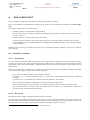
messages. In C++, messages correspond closely to (public) methods:
• as seen from the client side, the client sends a message: this means asking to another object to
execute one of its methods;
• as seen from the receiver side, the receiver object executes the corresponding (public) method.
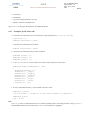
3.3.1.1
Example of collaborative work
A diffusive flux object (the sender) asks a k-l turbulent model object (the receiver) to perform its
method TurKL::compMut(). Here, the message corresponds to the method:
FxdFlux::message()
{
turObject -> compMut();
}
3.4
Class
A class is a prototype that defines the attributes and the methods common to all the instances of the class. The individual
instances are called objects. In practice, in C++, a new class is equivalent to a new type. A factory is used to manifacture
object instances from the class definition.
Note:
The factory itself may be an instance, (usually a unique one: a singleton) of a specialized class.
3.5
Inheritance
Object-Oriented programming allows classes to be defined in terms of other classes. For instance, class TurKL inherits
from class TurBase. TurKL is a subclass of the base class TurBase. Similarly, TurBase is the superclass (base
class) of all the classes in charge of turbulence modeling.
Inside inheritance tree, methods and data are inherited down through the levels:
• In abstract classes, methods are declared, but partially (or not) implemented. Abstract classes define the polymorphic behaviour: all the derived classes will provide this behaviour.
• Each subclass inherits attributes (state) and methods (behaviour) from the superclass.
– Subclasses can add their own data and methods to data and methods inherited from the superclass.
– Subclasses can override (that is, specialize) virtual inherited methods by providing specialized implementations for those methods.
elsA
DSNA
Design and Implementation Tutorial
Ref.: /ELSA/MDEV-06001
Version.Edition : 1.0
Date : Jan 10, 2006
Page :
17 / 75
– When implementing a new specialized subclass, developers can reuse the code (the implementation) defined
in superclasses. However, inheritance is really much more powerful than code factoring, which is of course
available in any decent language (C and Fortran, for exemple). With the help of inheritance, developers can
reuse the interface.
Inheritance greatly simplifies the software extensibility and maintenance tasks. The most important polymorphic hierarchies in elsA are:
• Implicit algorithms (LhsBase and derived classes).
• Boundary conditions (BndBase and derived classes; see Bnd component).
• Turbulence models (TurBase and derived classes; see Tur component).
• "Operators" (fluxes and source terms) (OperBase and derived classes; see Oper component).
Basically, developing a new implicit algorithm, a new boundary condition, or a new turbulence model, amounts to very
similar tasks:
• Starting from the base class interface (public and protected), the developer must adapt it to his wishes; most
of the time, the interface changes are very limited (usually somme additional private attributes and a few private
implementation methods).
• The developer must implement the abstract method(s) specific to the hierarchy:
– compLhs() for the Lhs hierarchy;
– compBoundaryValue(...) for the Bnd hierarchy (see How to introduce a new boundary condition?);
– compMutInModel() for the Tur hierarchy (see How to introduce a new turbulent model?).
– compInterior() for the OperFlux hierarchy.
3.6
And see other examples:
http://www.softwaredesign.com/objects.html
Ref.: /ELSA/MDEV-06001
Version.Edition : 1.0
Date : Jan 10, 2006
Page :
18 / 75
elsA
Design and Implementation Tutorial
4.
GENERAL ARCHITECTURE
4.1
elsA library and applications
DSNA
elsA provides an Object-Oriented (OO) CFD library. together with a stand-alone application elsA.x, using Python
as scripting language.
4.1.1
Object-Oriented architecture
elsA design and implementation are based both on Object-Oriented technology:
• elsA design uses the UML (Unified Modeling Language) modeling approach to obtain an accurate decomposition
of the complex CFD problem into static classes, and to model the dynamic interacting objects (instances of classes).
• elsA kernel is implemented in the Object-Oriented language C++. Only the most CPU time-consuming computing
loops are coded in Fortran, without impairing in any way the OO design.
4.1.1.1
elsA extensibility
elsA Object-Oriented architecture improves software extensibility through two basic mechanisms:
• polymorphism: developers can design and implement new features, such as a new turbulence model, a new
boundary condition, a new implicit time integration algorithm,... in an independent way. By this we mean that
code is extended through addition of new files, not modified, thus greatly decreasing integration time, by removing
any conflicts.
• encapsulation: Object-Oriented technology encourages a clear distinction between private and public part of a
component. Clients of the component only use the public interface, so they will not be affected by any changes in
the private (implementation) part of the component. This greatly reduce maintenance costs.
4.1.2
elsA input data
To run a computation, elsA users must provide:
• geometric data, basically mesh coordinates (and possibly geometric coefficients in chimera);
• topological data: connectivity between blocks;
• physical data, to initialize the time-iterative loop; this physical data may be a constant thermodynamic state, or,
more generally, come from data file (restart file).
• definition of boundary conditions; this may be only a boundary type identifier, or additional data may be needed
(for example transition data can be prescribed in a fully general way with additional files).
4.1.2.1
Definition of mesh points
Mesh generation is not addressed by elsA: users must provide mesh point coordinates, as computed from external tools
such as ICEM-CFD or NUMECA IGG 1 .
1
Note however that mesh deformation algorithms are available (ALE, fluid-structure coupling.
elsA
DSNA
Design and Implementation Tutorial
Ref.: /ELSA/MDEV-06001
Version.Edition : 1.0
Date : Jan 10, 2006
Page :
19 / 75
A mesh file (binary, or ASCII Tecplot format) must be associated with each block. This greatly simplifies the parallel
treatment, and is inherently scalable to massively parallel computations. To improve ergonomy, it is advised to put all
mesh files in a single directory, and to use a consistent file naming. In that case, users do not have to care about the
potentially large number of files, they are only aware of the directory name, which is just a "super-file".
4.1.2.2
Restart files
We use exactly the same mechanism as for mesh files. Again, the individual files associated with each block can be
grouped into a single directory.
4.1.2.3
Boundary information
The generation of the complete boundary definition information can be time consuming and error prone. An automatic
script generator is available to generate this information from ICEM-CFD input. It is often convenient to put boundary
definition in a separate Python script file (module), which is imported by the main (driver) script:
• boundary definition are nearly always kept unchanged;
• several computations ( with different numerical parameters, or Mach number,...) can share boundary definition,
thus avoiding potential errors when duplicating boundary data.
4.1.2.4
DAMAS database
A tool using as input a DAMAS database is also available.
Note:
In future releases, it will be optionnaly possible to read mesh coordinates, as well as restart data and boundary
definition data (at least for the "usual" boundary types) directly from a CGNS database.
4.1.3
Simulation control
elsA users control their CFD simulations through the Python scripting interface. This can be done in three ways:
• interactive text mode; this is limited to very basic test cases.
• through a Graphical User Interface (GUI), called PyGelsA, documented in the PyGelsA Graphical User interface User’s Manual (http://elsa.onera.fr/ExternDocs/user/MU-02044.pdf).;
• through a Python script file; this is the preferred way for complex simulations. It is fully described in the elsA
User Reference Manual (http://elsa.onera.fr/elsA/doc/refdoc.html).;
Using Python as the scripting interface greatly reduces the time required to develop and maintain the user interface.
Moreover, Python provides with a high level versatile programming interface, allowing novice as well as expert users to
interact with elsA in an optimized way. Let us give a small (non exhaustive!) list of useful Python features in the context
of CFD simulation:
• Script files can be splitted in several modules, allowing reuse of well-tested blocks of settings, thus avoiding many
potential errors.
• Simple Python programming enables basic numerical treatment in pre- or post-processing phase, such as normalization, directly in the script file, thus again avoiding inconsistent data arising from incompatible data coming from
different independent tools.
Ref.: /ELSA/MDEV-06001
Version.Edition : 1.0
Date : Jan 10, 2006
Page :
20 / 75
elsA
Design and Implementation Tutorial
DSNA
• Users can write specific functions, or even Python classes, to automate specific tasks.
• Users can benefit from the large number of additional scientific Python modules available.
4.1.3.1
Default value mechanism
Users are not required to set explicitly all the control data necessary to define completely a simulation. Default parameters
are provided through Python dictionary. The complete set of default parameters can be customized to suit the requirements
specific to a specific user community. Python dictionaries can be modified at any time, thus allowing dynamic site
customization without code recompilation.
4.1.3.2
Connecting Python and C++: Use of SWIG
elsA can be viewed as a standard Python module, elsA.py: it can be imported, as any other Python module. The task
of generating the "glue" code necessary to acces C++ code from the Python interpreter is done automatically by swig , a
public domain tool (cf. 13, p. 68).
4.1.4
Parallel mode
elsA can run in parallel, using MPI communication library. elsA uses a coarse-grained parallelization strategy: taking
advantage of elsA multiblock capability, each processor is responsible for the computation of a subset of the blocks
belonging to the configuration. elsA uses the SPMD (Single Program Multiple Data) paradigm:
• each executable runs exactly the same program, reading the same Python scripting file (Python interpreter is
embedded inside each parallel executable);
• each executable is responsible for local file pre- and post-processing: for example, if block 3 and 5 are allocated
to processor 2, processor 2 is responsible for reading mesh data files corresponding to blocks 3 and 5. This
should avoid bottleneck problems arising from centralized I/O treatment (for example through rank 0 processor)
in massively parallel computations.
The mapping between blocks and processors can be done either "manually, or with the Split module. To achieve
acceptable load balancing, splitting the initial configuration in a larger number of blocks may be necessary. This optional
splitting stage can also be done through the Split module.
4.1.5
Multidisciplinary Coupling
Several coupling strategies can be used to couple elsA with other computational software. Let us give several examples:
• External coupling, basically through file exchange, with elsA used in black box:
– in an optimization chain;
– weak coupling with the boundary layer code COULEUR;
– weak coupling with NASTRAN (static aeroelastic wing deformation computation).
• Use of a dedicated coupler, such as CALCIUM or PALM . A small number of "plugging" points have been identified and implemented inside elsA and tested.
• Modification of the internal algorithmic structure, to obtain full control and efficiency. This has been realized for
complex fully coupled aeroelastic simulations.
• elsA has been coupled with the structural mechanics code HOST , using a proprietary protocol based on CGNS
semantics.
elsA
DSNA
4.1.6
Design and Implementation Tutorial
Ref.: /ELSA/MDEV-06001
Version.Edition : 1.0
Date : Jan 10, 2006
Page :
21 / 75
Optimization module Opt
The Opt module implements the discrete Adjoint approach. It has been used inside automatic aerodynamic shape optimization process.
4.1.7 Access to CFD databases (CGNS, DAMAS)
indexdatabase (CFD)@database (CFD) To be written
4.1.8 Log file
For each run, elsA generates a log file (standard output), with some basic information:
• elsA version.
• precision (single or double precision)
• compiler options (DEBUG or optimized version)
• warning, or errors, if any.
Additionaly, users can augment the log file by a large number of additional output: in fact, most post-processing available
in elsA can be output either to a specific file, or to the log file.
Note:
In parallel mode, to avoid a "scrambled" log file (on some platforms, all the computing processors write in an essentially random order), there is one log file associated with each processor, with some information given only by the
root (rank 0) processor.
4.1.9 Post-processing
4.1.9.1 Restart files can be generated by specifying a directory name.
This directory can then be used as input for a subsequent computaion.
4.1.9.2 Global residuals
With default parameter GLOBAL_RESIDUAL set to YES, residuals for the complete configuration are automatically
extracted.
4.1.9.3
General post-processing
A very fine control of post-processing is available.
• Local quantities: a wide range of local quantities (Mach, pressure,...) can be extracted.
• Global quantities: global quantities (lift, drag, mass flow, residuals,...) are available, with a simplified syntax when
defined on predefined window families (for example, one family may correspond to the wing, another one to the
fuselage).
Ref.: /ELSA/MDEV-06001
Version.Edition : 1.0
Date : Jan 10, 2006
Page :
22 / 75
elsA
Design and Implementation Tutorial
5.
KERNEL DESIGN
5.1
Classification and Design organization
DSNA
CFD concepts can be classified as: geometrical, topological, numerical and physical concepts. In order to solve a CFD
problem, we have defined a limited number of basic classes responsible of the following actions:
1. to take into account the fluid physical properties in the flow;
2. to build and control the numerical space region where the system of equations is solved;
3. to build the system of equations: compute the terms arising from the spatial discretization (flux, source terms);
controls the application of the boundary conditions;
4. to control the time evolution of the solution.
So, the kernel has been designed as a set of consistent modules (or components). A module is responsible for a set
of well-defined functionalities. Ideally, developers should be able to work inside a module, without having to know the
implementation details of any other modules. Achieving a good decomposition is very important to improve ease of
development and maintenance.
Moreover, this OO model has been split into sub-models with the aim to keep dependencies as local as possible. These
modules are organized into layers in such a way that each layer should only affect the layers above. The goal of this
organization is to achieve mono-directional relationships. The advantage is then that the maintenance becomes much
easier, since one layer’s interface affects only the upper layers. Avoiding cyclic dependency greatly simplify test policy.
5.1.1
Naming convention
Each module is identified by a key of 3 to 5 letters, the first one being capitalized. Inside each module, each class name is
then prefixed by the key of the module it belongs to. Example: TurKL belongs to the Tur module.
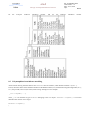
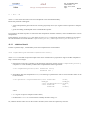
5.2
Overview of the layers
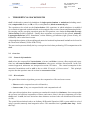
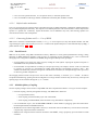
elsA kernel includes about 400 classes grouped in 26 modules specialized for a given CFD task. These modules are further
organized in 6 layers:
• Base;
• Geometry;
• Physical model;
• Space Discretization;
• Solver;
• Factory (top level).
elsA
DSNA
Design and Implementation Tutorial
Ref.: /ELSA/MDEV-06001
Version.Edition : 1.0
Date : Jan 10, 2006
Page :
23 / 75
Ref.: /ELSA/MDEV-06001
Version.Edition : 1.0
Date : Jan 10, 2006
Page :
24 / 75
5.2.1
elsA
Design and Implementation Tutorial
DSNA
Base layer
Base layer gathers all low-level modules, among which the Fld and Pcm modules.
• Fld: data storage classes; these classes encapsulate dynamic memory needed to store any computational data.
Their interface provide with monitoring methods, optimized array-like syntax (much like FORTRAN 90) and
methods to communicate with FORTRAN routines. Fld classes are built in order to provide the highest efficiency
(both in CPU and memory); a comparable efficiency could not be achived through STL containers.
• Pcm: deals with parallel implementation; it "encapsulates" message passing interface (presently, MPI).
5.2.2
Geometry layer
Geometry layer gathers all geometrical and topological modules:
• Blk: defines the block notion. A block corresponds to a region of the discretized physical space defined by a
mesh, to which are associated boundary and initial conditions. Blocks are specialized to take into account grid
motion, ALE, chimera and HMR (Hierarchical Mesh Refinement) features. In most simulations, several blocks
are needed.
• Geo: defines the abstraction of the computational grid; provides all geometrical ingredients used by a finite
volume formulation:
– Metrics: volume of cells, surface of cell interfaces.
– Topological relations between geometrical entities: cells, interfaces, nodes. Recently, ghost cells have been
introduced in elsA. Thanks to these ghost cells, most indirections have been suppressed in computational
loops, and important improvement in CPU efficiency has been obtained.
• Dtw: gathers all distance and boundary-layer integral thickness computations.
• Mask: defines concepts used in the Chimera technique.
• Join: deals with multi-block computations. Multi-zone interface connectivity can be 1-to-1 abutting, 1-to-n
abutting, or mismatched abutting.
5.2.3
Physical model layer
It includes two modules:
• Eos: computes quantities such as pressure,temperature, laminar viscosity;
• Tur: deals with turbulence modeling and transition prediction.
5.2.4
Space Discretization layer
This layer is responsible for the computation of the equation terms and of the boundary conditions:
• Oper: each operator class is responsible for the computation of a single term in the CFD equations:
– Fxc: convective fluxes;
– Fxd: diffusive fluxes;
– Sou: source terms.
• Bnd: deals with boundary conditions.
elsA
DSNA
5.2.5
Design and Implementation Tutorial
Ref.: /ELSA/MDEV-06001
Version.Edition : 1.0
Date : Jan 10, 2006
Page :
25 / 75
Solver layer
This layer is responsible for:
• Rhs: builds the right hand side of the equation system;
• Lhs: gathers implicit methods; each implicit class has to build and invert the matrix resulting from a specific
linearization of the system of equations;
• Tmo: time integration module; manages the main iterative (pseudo-)time loop.
It is probably the most complex part of the kernel, since many algorithms have to be taken into account: multi-block,
multigrid, HMR, mesh motion, deformation, ...
5.2.6
Factory layer (elsA top layer)
This layer is responsible of the dynamic creation of all kernel objects: the Fact module implements several object
"factories" to build object instances from user input data coming from the Python interface.
Ref.: /ELSA/MDEV-06001
Version.Edition : 1.0
Date : Jan 10, 2006
Page :
26 / 75
6.
FLD COMPONENT
6.1
Basic numerical containers
elsA
Design and Implementation Tutorial
DSNA
Fields are the most basic objects manipulated by elsA. They are used as containers for the numerical values (real, integer,
boolean) arising in CFD simulations.
It is useful to distinguish two general types:
• FldArray : stores numeric values, without any location information;
• FldField : stores numeric values defined on a grid. In that case, it can be also very useful to distinguish between:
– values defined at grid nodes: FldNode;
– values defined at centers of grid cells: FldCell;
– values defined at centers of grid interfaces: FldInt.
So, we use typedef to express the specificity of each entity; for example:
typedef FldFieldF FldCellF;
This automatically gives important information upon the programmer’s intent, and so facilitates code understanding and maintenance.
These containers must contain homogeneous collection of floats, integers, or booleans. To fulfill this requirement, elsA
provides different versions of FldArray and FldField; the last letter of the class name identifies the contained element
type:
• F stands for Float,
• I stands for Integer,
• B stands for Boolean.
Note:
FldFieldB is not implemented.
6.2 Public interface
Externally, for application programmers, fields are viewed as two-dimensional structures:
• the first dimension index goes from 0 to _size-1;
• the second dimension index goes from 1 to _nfld; if the second dimension is 1, it can be omitted.
Note:
The conventions used for first and second dimensions are inconsistent (0 instead of 1 for first index). This comes
from historical reasons, and may be changed in future releases (just modify the constant NUMFIELD0, defined in
FldArray.h, and recompile).
The field interface provides all the methods required to do numerical computations:
elsA
DSNA
Design and Implementation Tutorial
Ref.: /ELSA/MDEV-06001
Version.Edition : 1.0
Date : Jan 10, 2006
Page :
27 / 75
• construction;
• initialization;
• copy of an existing field into a new one;
• addition, subtraction, multiplication.
(See FldFieldF doxygen documentation for additional details).
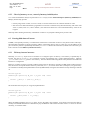
6.2.1
Examples of Fld client code
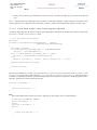
1. Construction of a field which stores the unknowns of the CFD problem (ro, rou, rov, row, roE):
E_Int nfld = 5;
FldCellF wCons(ncell, nfld);
Construction of a field which stores fluxes:
FldIntF flux(3*ncell, nfld);
2. Construction of a field which stores mesh coordinates:
FldNodeF x(ncell, 3);
FldNodeF y(ncell, 3);
FldNodeF z(ncell, 3);
3. FldArray or FldField can be used to store values without geometric links, such as:
FldArrayF TurKO::getModConst() const
{
FldArrayF modConst (7);
modConst[0] = _kappa;
modConst[1] = _sigma1;
modConst[2] = _sigmae1;
modConst[3] = _beta1;
modConst[4] = _wsig1;
modConst[5] = _betae;
modConst[6] = _Sr;
}
4. To access individual elements, a syntax similar to Fortran is used:
FldArrayF f(100,2);
f(3,2)=3.14159; // assigns pi to the fourth element of component 2
FldArrayF g(100);
g[0] = 2.22;
Note:
FldArray is really an implementation class; it would be probably better to avoid using it directly, using FldField
instead (additional memory associated with FldField own attributes is negligible).
Ref.: /ELSA/MDEV-06001
Version.Edition : 1.0
Date : Jan 10, 2006
Page :
28 / 75
6.2.2
elsA
Design and Implementation Tutorial
DSNA
Check of memory access, control of memory initialiazation
Fld classes should almost always be preferred to C/C++ arrays (see also Prefer Fld objects (FldArray, FldField) to C
arrays), because they provide:
• memory usage check control; in DEBUG mode, we can check that access to container elements is valid:
• full control over data initialization; programmers can choose to initialize newly allocated memory with some "bad
value" or, better, with Nan ("Not a number"); this will insure that access to non-initialized memory value can be
trapped.
Subscript index checking and memory initialization control are very helpful to debug newly written code.
6.3
Passing field data to Fortran
In elsA, it is frequenltly necessary to communicate with Fortran 77 subroutine. Fortran 77 only knows scalars and arrays,
and subroutine arguments are always passed by address. This means that we must, in some way, give the address of the
piece of memory which is dynamically allocated by a FldField field to this subroutine (to know more about that, just
look at the next section FldArray internal structure).
6.3.1
FldArray internal structure
Internally, a FldArray object stores its elements in a contiguous piece of memory. This memory is dynamically allocated. One can see FldArray as a convenient "wrapper" encapsulating raw C pointer-managed memory. Attribute
_data in class FldArray points to this memory. This one-dimensional arrangement exactly matches the traditional
Fortran or C arrangement.
However, it remains to choose a specific ordering between the two directions. Presently in elsA, the first index increases
first; this choice corresponds to the Fortran way. Note that, in C++, we can turn to the other ("transpose") way quite easily:
we would have to modify the implementation of exactly one method, leaving the class interface strictly unchanged. Instead
of:
inline E_Float
FldArrayF::operator()(E_Int l, E_Int fld) const
{
return (_data[l + (fld-1)*_size]);
}
We would have the transpose (or swapped) implementation:
inline E_Float
FldArrayF::operator()(E_Int l, E_Int fld) const
{
return (_data[fld-1 + l*_nfld]);
}
When the elsA programmer uses a Fld object, he uses the public class interface, so he doesn’t know how the data are
actually stored and he should not be "disturbed" by any modification of the internal structure of the Fld classes. In Fortran
obviously, it is another matter...
elsA
DSNA
6.3.2
Design and Implementation Tutorial
Ref.: /ELSA/MDEV-06001
Version.Edition : 1.0
Date : Jan 10, 2006
Page :
29 / 75
Examples
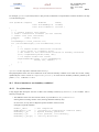
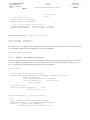
If called from inside a C++ method, a Fortran subroutine has first to be declared in a prototype, such as 1 :
extern "C"
{
void
denconvec_(const E_Int& ncell, const E_Int& neqtot, const E_Int& neq,
const E_Int& ro, const E_Int& rou, const E_Int& roe,
const E_Int& rog, const E_Int& roug, const E_Int& roeg,
const E_Float* consvar, const E_Float* press,
E_Float* fdx, E_Float* fdy, E_Float* fdz);
}
It is important to note that each argument is passed by address (reference for scalar, pointer for array), not by value (see
Calling Fortran subroutine).
Then, in the C++ method, the Fortran subroutine is called by:
denconvec_(ncell, neqTot, nbEqMoyComp,
rho, mom, ene, rhoG, momG, eneG,
wCons.begin(), press.begin(),
fdx.begin(), fdy.begin(), fdz.begin() );
The use of fdX.begin() allows to point on the begining of the piece of memory where the values of the field fdX
are stored. To get this address, it is convenient to use the iterator mechanism whose member functions are begin(),
end().
Notation: fdX.begin() stands for fdX.begin(1) (1 is the default value). If it is needed to manipulate the second
field (corresponding to rou) the method begin has to be used with the argument 2: fdX.begin(2).
It is obvious to see that if we change the two-dimensional structure choice (first index increases first), the method begin() will not provide the same collection of entities. In this case, and if dimensions of fdX are: ncell x neq, values
of fdX will be stored in the following order:
fdX(
0,1), fdX(0,2), fdX(0,3),..., fdX(
0,neq),
...,
fdX(ncell-1,1), ...,
fdX(ncell-1,neq)
instead of:
fdX(0, 1), fdX(1,1),fdX(2,1),..., fdX(ncell-1, 1),
...,
fdX(0,neq),...,
fdX(ncell-1,neq)
Finally, in the Fortran subroutine, we find the following implementation:
SUBROUTINE denconvec(ncell, neqtot, neq,
&
ro, rou, roe,
&
rog, roug, roeg,
1
See also "elsA Coding Rules"
Ref.: /ELSA/MDEV-06001
Version.Edition : 1.0
Date : Jan 10, 2006
Page :
30 / 75
&
&
IMPLICIT NONE
elsA
Design and Implementation Tutorial
w, p,
fdx, fdy,
DSNA
fdz)
C_IN
INTEGER_E ncell, neqtot, neq
REAL_E
w(0:ncell-1,neqtot)
REAL_E
p(0:ncell-1)
! Conservative Variables
! Pressure
REAL_E
REAL_E
REAL_E
! Convective Flux
! Convective Flux
! Convective Flux
C_OUT
fdx(0:ncell-1,neq)
fdy(0:ncell-1,neq)
fdz(0:ncell-1,neq)
X-Component
Y-Component
Z-Component
[.......]
DO icell = 0, ncell-1
roi = ONE / w(icell,rog)
fdx(icell,ro)
fdy(icell,ro)
fdz(icell,ro)
[.......]
6.3.3
= w(icell,roug)
= w(icell,rovg)
= w(icell,rowg)
Remark on Fortran convention
In the example above, the following convention has been followed in the two-dimensional array addressing:
• the first dimension index varies from 0 to ncell-1;
• the second dimension index varies from 1 to neq.
This choice has been made here in order to be the same as the C++ choice, but it is not mandatory. We could of course
also write:
...
REAL_E
w(ncell,neqtot)
REAL_E
REAL_E
REAL_E
fdx(ncell,neq)
fdy(ncell,neq)
fdz(ncell,neq)
C_OUT
[.......]
DO icell = 1, ncell
roi = ONE / w(icell,rog)
fdx(icell,ro)
fdy(icell,ro)
fdz(icell,ro)
[.......]
= w(icell,roug)
= w(icell,rovg)
= w(icell,rowg)
elsA
DSNA
Design and Implementation Tutorial
Ref.: /ELSA/MDEV-06001
Version.Edition : 1.0
Date : Jan 10, 2006
Page :
31 / 75
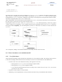
GEO COMPONENT
7.
GeoGrid objects are widely used in the CFD kernel, because many CFD classes need a pointer on GeoGrid objects.
GeoGrid is a composition of two classes: GeoGridMetrics and GeoConnect. It is responsible for:
• metrics, issued from methods of GeoGridMetrics class;
• index counting and position (connectivity), issued from methods of GeoConnect class.
7.1
Ghost geometric entities
The number of ghost entities is controlled through 6 global variables:
GHOST_I1 and GHOST_I2 in the "I" direction,
GHOST_J1 and GHOST_J2 in the "J" direction,
GHOST_K1 and GHOST_K2 in the "K" direction.
elsA uses the following convention:
7.1.1
Ghost cell numbering
• GHOST_I1 ghost cells in IMIN, GHOST_I2 ghost cells in IMAX,
• GHOST_J1 ghost cells in JMIN, GHOST_J2 ghost cells in JMAX,
• GHOST_K1 ghost cells in KMIN, GHOST_K2 ghost cells in KMAX.
7.1.2
Ghost interface numbering
• GHOST_I1 ghost interfaces in IMIN, GHOST_I2-1 ghost interface in IMAX,
• GHOST_J1 ghost interfaces in JMIN, GHOST_J2-1 ghost interface in JMAX,
• GHOST_K1 ghost interfaces in KMIN, GHOST_K2-1 ghost interface in KMAX.
7.1.3
Ghost node (mesh points) numbering
• GHOST_I1 ghost nodes in IMIN, GHOST_I2-1 ghost node in IMAX,
• GHOST_J1 ghost nodes in JMIN, GHOST_J2-1 ghost node in JMAX,
• GHOST_K1 ghost nodes in KMIN, GHOST_K2-1 ghost node in KMAX.
7.1.3.1
Ghost defaultvalues
The default values are:
GHOST_I1 = 2; GHOST_I2 = 2;
GHOST_J1 = 2; GHOST_J2 = 2;
GHOST_K1 = 2; GHOST_K2 = 2;
Ref.: /ELSA/MDEV-06001
Version.Edition : 1.0
Date : Jan 10, 2006
Page :
32 / 75
elsA
Design and Implementation Tutorial
DSNA
Users can change these default values at the beginning of each run by calling DesCfdPb::set_ghostcell() (usually to reduce CPU time on some platforms).
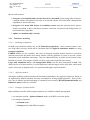
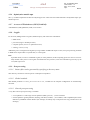
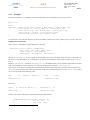
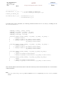
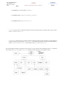
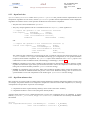
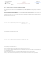
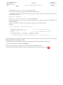
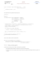
7.1.4
Simplified example
We give here a simple example, where the "k" planes have been neglected:
7.1.5
Identical numbering of cell / interface / node
The benefit of this choice is that we have a simple relation between cell, interface and node indexes, which enables easy
looping over cells, interfaces or nodes.
DO n=n0cell, nfcell
ni1 = n
nj1 = n +
ncell
nk1 = n + 2*ncell
....
ni2 = n +
inccell(1,0,0)
nj2 = n +
ncell + inccell(0,1,0)
nk2 = n + 2*ncell + inccell(0,0,1)
!
!
!
!
loop on cells
"i" interface (left)
"j" interface (down)
"k" interface (back)
! "i" interface (right
! "j" interface (up)
! "k" interface (front)
As a consequence of this choice, we have exactly the same number of cells, nodes, and interface in direction I, J or K (so,
the total number of interfaces is three time the number of cells).
inline E_Int
elsA
DSNA
Design and Implementation Tutorial
Ref.: /ELSA/MDEV-06001
Version.Edition : 1.0
Date : Jan 10, 2006
Page :
33 / 75
GeoConnect::getNbCell() const
{
return ((_im - 1 + GHOST_I1 + GHOST_I2)*
(_jm - 1 + GHOST_J1 + GHOST_J2)*
(_km - 1 + GHOST_K1 + GHOST_K2));
}
inline E_Int
GeoConnect::getNbInti() const
{
return getNbCell();
}
7.2
Address and increment methods
The expression of the address methods is directly issued from the following points:
• by convention:
– the first "real" (non ghost) cell corresponds to (1,1,1);
– the IMIN (left) I interface of cell (1,1,1) corrsponds also to (1,1,1);
– the JMIN (lower) J interface of cell (1,1,1) corrsponds also to (1,1,1);
– the KMIN (back) K interface of cell (1,1,1) corrsponds also to (1,1,1);
• ghost geometric entities have to be taken into account; for example, the indices of the two "extreme" cells are:
imin = - GHOST_I1 + 1; imax = im -1 + GHOST_I2;
jmin = - GHOST_J1 + 1; jmax = jm -1 + GHOST_J2;
kmin = - GHOST_K1 + 1; kmax = km -1 + GHOST_K2;
• data are always stored first considering the "i"-direction, then the "j"-direction, and lastly the "k"-direction;
• in the case of interfaces, we first consider the "i"-interfaces (for "i", then for "j", then for "k"), then the "j"-interfaces
(for "i", "j", "k"), and finally the "k"-interfaces (for "i", "j", "k");
Address methods dealing with index counting and position, which are available in class GeoConnect, must be used in
all the C++ kernel classes. If im, jm, km are the number of mesh points in the directions "i", "j", "k", then the numbering
of cells, nodes, interfaces in the total grid (real + ghost entities) are:
Address methods:
----------------adrCell(i,j,k) = i - 1 + GHOST_I1
+(j - 1 + GHOST_J1)*(im -1 + GHOST_I1 + GHOST_I2)
+(k - 1 + GHOST_K1)*(im -1 + GHOST_I1 + GHOST_I2)
*(jm -1 + GHOST_J1 + GHOST_J2)
adrInti(i,j,k) = adrCell(i,j,k)
adrIntj(i,j,k) = adrCell(i,j,k) + nCell
adrIntk(i,j,k) = adrCell(i,j,k) + 2*nCell
adrNode(i,j,k) = adrCell(i,j,k)
Increment methods:
Ref.: /ELSA/MDEV-06001
Version.Edition : 1.0
Date : Jan 10, 2006
Page :
34 / 75
elsA
Design and Implementation Tutorial
DSNA
-----------------incrementCell (i,j,k) = i + j*( im-1+GHOST_I1+GHOST_I2)
+ k*((im-1+GHOST_I1+GHOST_I2)*(jm1+GHOST_J1+GHOST_J2))
increment[IJK](i,j,k) = incrementCell(i,j,k)
= incrementNode(i,j,k)
If needed inside Fortran subroutines, the following statement functions have to be used, by including the file
Geo/Grid/GeoAdrF.h"
INTEGER_E
INTEGER_E
INTEGER_E
INTEGER_E
idummy, jdummy, kdummy
im_dummy, jm_dummy, km_dummy
adrcell, adrcellg, inccellg
adrnodeg, incnodeg
adrcellg(idummy,jdummy,kdummy, im_dummy, jm_dummy, km_dummy) =
&
(idummy-1+IFIC1)
&
+ (jdummy-1+JFIC1)*(im_dummy-1+IFIC1+IFIC2)
&
+ (kdummy-1+KFIC1)*(im_dummy-1+IFIC1+IFIC2)*
&
(jm_dummy-1+JFIC1+JFIC2)
adrnodeg(idummy,jdummy,kdummy, im_dummy, jm_dummy, km_dummy) =
&
(idummy-1+IFIC1)
&
+ (jdummy-1+JFIC1)*(im_dummy-1+IFIC1+IFIC2)
&
+ (kdummy-1+KFIC1)*(im_dummy-1+IFIC1+IFIC2)*
&
(jm_dummy-1+JFIC1+JFIC2)
incnodeg(idummy,jdummy,kdummy, im_dummy,jm_dummy,km_dummy)=
&
idummy
&
+ jdummy*(im_dummy-1+IFIC1+IFIC2)
&
+ kdummy*(im_dummy-1+IFIC1+IFIC2)*(jm_dummy-1+JFIC1+JFIC2)
inccellg(idummy,jdummy,kdummy, im_dummy,jm_dummy,km_dummy)=
&
idummy
&
+ jdummy*(im_dummy-1+IFIC1+IFIC2)
&
+ kdummy*(im_dummy-1+IFIC1+IFIC2)*(jm_dummy-1+JFIC1+JFIC2)
These methods (address and increment) allow to deal with connectivity between cells and interfaces as it is usual in finite
volume formulation.
Note:
adrcellg (adrnodeg, adrintg) will be renamed as adrcell (respectively adrnode, adrint) in future
releases.
elsA
DSNA
7.2.1
Design and Implementation Tutorial
Ref.: /ELSA/MDEV-06001
Version.Edition : 1.0
Date : Jan 10, 2006
Page :
35 / 75
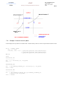
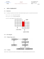
Example: Centered convective fluxes
In this example, the loop index is an interface index. Cell flux density values are used to compute the flux interface values.
DO n
= n0Int, nfInt
int = n + incI
flux(int, fld) = 1/2 * [Qx(n,fld)+Qx(n-inc,fld)]*surfx(int,1)
+ [Qy(n,fld)+Qy(n-inc,fld)]*surfy(int,1)
+ [Qz(n,fld)+Qz(n-inc,fld)]*surfz(int,1)
END DO
with:
interfaces "I"
-------------inc = 1 = inccell(1,0,0, im,jm,km)
incI = 0
interfaces "J"
-------------inc = im-1+GHOST_I1+GHOST_I2 = inccell(0,1,0, im,jm,km)
incI = nCell
interfaces "K"
-------------inc = (im-1+GHOST_I1+GHOST_I2)*(jm-1+GHOST_J1+GHOST_J2)
= incell(0,0,1, im,jm,km)
incI = 2*nCell
Ref.: /ELSA/MDEV-06001
Version.Edition : 1.0
Date : Jan 10, 2006
Page :
36 / 75
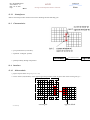
7.2.2
elsA
Design and Implementation Tutorial
DSNA
Example: Flux balance
In this example, the loop index is a cell index. Interface flux values are used to compute the cell flux balance values.
l1 = 1
= inccell(1,0,0, im,jm,km)
l2 = im-1+GHOST_I1+GHOST_I2
= inccell(0,1,0, im,jm,km)
l3 = l2*(jm-1+GHOST_J1+GHOST_J2) = inccell(0,0,1, im,jm,km)
DO n
= n0Cell, nfCell
intI = n
intJ = n +
nCell
intK = n + 2*nCell
fluxBal(n,nfld) = + flux(intI + l1, fld)
- flux(intI
, fld)
+ flux(intJ + l2, fld)
- flux(intJ
, fld)
+ flux(intK + l3, fld)
- flux(intK
, fld)
END DO
elsA
DSNA
Design and Implementation Tutorial
8.
TUR COMPONENT
8.1
Definition of the public interface
Ref.: /ELSA/MDEV-06001
Version.Edition : 1.0
Date : Jan 10, 2006
Page :
37 / 75
This section details the design of the turbulence models based on the Boussinesq hypothesis.
The most important design activity is to identify the classes, together with their public interface. The UML class diagram
is a very useful tool to present:
• classes;
• relations between classes;
• interfaces.
The first analysis stage is to identify what actions turbulence models are responsible for. The aim of turbulence models is
to compute:
• turbulent eddy viscosity;
• total stress tensor (viscosity tensor + Reynolds tensor) used in momentum and energy equations;
• possibly other quantities needed for the integration of transport equations (source terms, coefficients for the
computation of the density of the diffusive turbulent fluxes).
Moreover, the design solution must allow association of transition with any turbulence model.
More precisely, depending on algebraic model or transport equation model, we have to distinguish which computations
have to be made and how they can be made :
• for algebraic models,the computation of the eddy viscosity only requires the knowledge of the conservative variables and the distance to wall;
• for turbulence models using transport equations, a system of equations must be integrated. Source terms, additional
coefficients needed to compute the diffusive fluxes, and also eddy viscosity have to be computed.
This analysis shows that the public methods of the turbulence component interface (Object-Oriented Programming
Concepts ) are:
1. compute the eddy viscosity;
2. compute the total stress tensor;
3. apply transition.
Methods 2 and 3 can be defined in the same way whatever turbulence model; conversely, it is clear that the eddy viscosity
implementation depends on the model.
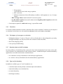
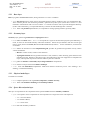
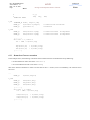
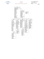
8.2
Class model
Finally, we obtain the following UML class diagram which presents a tree hierarchical structure organization:
• TurBase is the base abstract class; its interface declares:
– the pure virtual method compMutInModel();
Ref.: /ELSA/MDEV-06001
Version.Edition : 1.0
Date : Jan 10, 2006
Page :
38 / 75
elsA
Design and Implementation Tutorial
DSNA
– the concrete (non virtual) method compMut();
– the concrete method compDiffFluxDens_gradCen().
– the concrete method applyTransition();
• TurAlg is the base class for algebraic turbulence models; the derived classes provide the eddy viscosity computation (compMutInModel());
• TurTransp is the base class for transport equation turbulence models; the derived classes provide methods to
compute the source terms (method compSource()), the coefficients needed to compute the turbulent diffusive
fluxes (compDifFluxDensCoef()) and the eddy viscosity (compMutInModel()).
The actual turbulence models correspond to concrete classes. All the concrete classes belonging to the Tur component
inherit either from TurAlg or from TurTransp, depending of their algebraic (or non algebraic) nature.
elsA
DSNA
Design and Implementation Tutorial
Ref.: /ELSA/MDEV-06001
Version.Edition : 1.0
Date : Jan 10, 2006
Page :
39 / 75
Ref.: /ELSA/MDEV-06001
Version.Edition : 1.0
Date : Jan 10, 2006
Page :
40 / 75
elsA
Design and Implementation Tutorial
DSNA
elsA
DSNA
transport
Ref.: /ELSA/MDEV-06001
Version.Edition : 1.0
Date : Jan 10, 2006
Page :
41 / 75
Design and Implementation Tutorial
for
the
equations
turbulence
models,
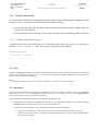
8.3
Polymorphism in turbulence modeling
and
for
the
algebraic
turbulence
models.
All the classes deriving from the abstract class TurBase share its interface, which declares method compMut().
In elsA, the client classes of the turbulence models are the diffusive fluxes (Fxd) and the time integration algorithm (Tmo);
Tur (the provider) and Fxd (the client) interact using "messages" as for example:
_tur->compMut(...);
where _tur is an attribute of type TurBase∗ belonging to this Fxd object. TurBase::compMut() is a concrete
method which consists of two stages:
TurBase::compMut()
{
Ref.: /ELSA/MDEV-06001
Version.Edition : 1.0
Date : Jan 10, 2006
Page :
42 / 75
elsA
Design and Implementation Tutorial
DSNA
compMutInModel();
applyTransition();
}
If transition has to be taken into account, the method applyTransition() applies the intermittency function on the
eddy viscosity, in a uniform way for all the models. The method applyTransition() is then a concrete method
implemented in TurBase. Conversely, computation of the eddy viscosity depends on each particular turbulence model,
and cannot be implemented in the TurBase abstract class.
When manipulated in term of this abstract interface defined by TurBase, the concrete classes have not to be known by
the client classes. Client classes are only aware of abstract class.
Polymorphism allows the correct version of compMutInModel() to be called dynamically, without any explicit
"switch" coding by the programmer. In the example discussed in the preceding sections of the Fxd/Tur interaction
through the method compMut(), the client manipulates a pointer (or a reference) to an instance of a class derived from
TurBase.
As a consequence, adding a new turbulence model will not modify the code of the client class.
8.4
How to introduce a new turbulent model?
8.4.1
Use of inheritance
Object-Oriented technology greatly facilitates the introduction of a new turbulence model. The developer does not have
to have full knowledge of the whole elsA kernel. Instead, he can focus on a small number of well-defined tasks:
• introduce a new class in the turbulence hierarchy, deriving from a base class:
– deriving from TurTransp, if it is a new transport equation model;
– deriving from TurAlg, if it is an algebraic model;
– or even deriving (specializing) from from an existing "leaf" concrete class, let’s say TurKL, to test some
specialized TurKL variant.
• implement a small number of virtual methods;
• additionaly, to ease implementation, it may be useful to introduce new private methods and/or attributes.
elsA
DSNA
Design and Implementation Tutorial
Ref.: /ELSA/MDEV-06001
Version.Edition : 1.0
Date : Jan 10, 2006
Page :
43 / 75
Hence, OO programming provides a simple framework, allowing the programmer to work in a faster and safer way.
It remains to be seen how turbulent objects are created. This is fully discussed in section Factory component.
Ref.: /ELSA/MDEV-06001
Version.Edition : 1.0
Date : Jan 10, 2006
Page :
44 / 75
elsA
Design and Implementation Tutorial
DSNA
OPER COMPONENT
9.
Operator classes are dedicated to the computation of space discretization terms. Every operator has to compute a FldFieldF object defined upon a specific geometric entity (cell or interface). This chapter is dedicated to all operators in
elsA:
• Oper: Abstract classes;
• Fxc: Convective fluxes (centered scheme, upwind schemes and artificial dissipation);
• Fxd: Diffusive fluxes (laminar, mean flow or turbulent);
• Sou: Source terms (turbulence closure relations, moving frame, dual time stepping method).
9.1
Oper Module
9.1.1
OperBase abstract class
The general operator mechanism is defined inside OperBase class. Important attributes of OperBase are:
• _geoEntity: type of geometric entity where the computation has to be carried out;
• _borderDepth: width of the "border" region. The numerical treatment of an operator is performed on all cells
or interfaces, using the same numerical scheme on all geometric entities. The "interior" region of the operator is
the set of the geometric entities where this "current entity" treatment is directly correct. The "border" region is
the set of geometric entities where a numerical adaptation (correction) has to be made because of the boundary
neighborhood.
• _elemSysOper: identifier of the system of equations.
The other attributes of this abstract class are pointers:
• EosSysEq∗ _sysEq: current description of the problem;
• EosIdealGas∗ _eos: current equation of state;
• GeoGridBase∗ _grid: current working computational grid.
An operator has to work on different contexts (different grids, thermodynamic model, ...), so an Oper object cannot be
fully configured at construction time. Instead, when context changes, it must be re-initialized in such a way that it can
work correctly. This is precisely the job of OperBase::prepare(), whose signature is:
virtual void prepare(const EosSysEq&, EosElemSysType,
EosIdealGas* eos, const GeoGridBase* grid);
The method implementation is very simple: it reduces to proper (re-)settings of the class pointer attributes.
We must clearly distinguish two different operator subtypes, both inheriting from OperBase class:
• OperTerm is responsible for the computation of one ’right hand side’ term;
• Utility operators are used to perform auxiliary computations; they are usually called by OperTerm objects. Up
to now, only two gradient operators have been implemented: OperGrad and OperGradInt.
elsA
DSNA
9.1.2
Design and Implementation Tutorial
Ref.: /ELSA/MDEV-06001
Version.Edition : 1.0
Date : Jan 10, 2006
Page :
45 / 75
OperGrad class
OperGrad and OperGradInt inherit from OperBase. OperGrad class provides with the implementation of the
computation of gradients on cell centers, whereas OperGradInt provides with the implementation of the computation
of gradients on interface centers. These operators do not own the result of their computation:
• They don’t have more attributes than OperBase.
• They only compute gradients with two overloaded versions of compute(), whose signature are:
// compute the gradient of the conservative variables
void compute(
FldCellF&
fldOut,
const list<BndPhys*>& listBnd,
const list<JoinBase*>& listJoin,
AuxField
identOfField = MISC);
and:
// compute the gradient of non conservative
virtual void compute(
FldCellF&
const list<BndPhys*>&
const list<JoinBase*>&
const FldCellF&
AuxField
variables (?)
fldOut,
listBnd,
listJoin,
fldIn,
identOfField);
The gradient or flux computation is performed on all cells or interfaces using the same numerical scheme, in the
interior and the border region. The standard formula may give wrong results (or even produce arithmetic
exception) for the border computation. So, operator objects must collaborate with boundary objects. This
collaboration can take two different forms (called Strategy 1 and Strategy 2, see also 10.1):
• Stategy 1: computation in two stages: Gradient or flux computation is performed on all cells or interfaces, including those from the border region. Then, special formula are used to correct the computation on the border region,
taking into account the boundary treatment. OperGrad uses this strategy.
• Strategy 2: computation in only one stage: Ghost cells are filled by boundary objects, before the gradient computation, such that the standard formula will give the correct result. Within this strategy, there is no need to use
special formula to correct the computation on the border region. OperGradInt uses this strategy.
9.1.3
OperTerm abstract class
Most of the time, an operator needs to compute some auxiliary fields before the final computation of fluxes or source term
(for example, the pressure field has to be computed to complete the centered convective flux computation). So, the stage
"Computation of an OperTerm" is split into two sub-stages:
1. computation of all the required auxiliary fields (by means of the conservative variables),
2. computation of fluxes or source terms (using these auxiliary fields).
Auxiliary fields which have to be computed before flux or source term computation have to be identified. A specific
attribute, OperTerm::_setOfIdent, of type list<AuxField>, is introduced to store auxiliary field identifiers.
The method:
virtual
void computeAllField(const list<BndPhys*>* listBnd = E_NULLPTR,
const list<JoinBase*>* listJoin = E_NULLPTR);
Ref.: /ELSA/MDEV-06001
Version.Edition : 1.0
Date : Jan 10, 2006
Page :
46 / 75
elsA
Design and Implementation Tutorial
DSNA
calls the computeField() method for each auxiliary field registered by _setOfIdent. Operators compute each
registered field through a call to computeField():
virtual
void computeField(AuxField
identOfField,
const list<BndPhys*>* listBnd = E_NULLPTR,
const list<JoinBase*>* listJoin = E_NULLPTR);
computeField() is pure virtual and must be implemented by concrete operators.
Fluxes or source term computation are not implemented at this level. This is discussed in the next sections.
9.1.4
OperFlux abstract class
OperFlux inherits from OperTerm. It implements the major computational method compute() according to Strategy
1:
void OperFlux::compute(
FldIntF&
fldOut,
const list<BndPhys*>& listBnd,
const list<JoinBase*>* listJoin )
{
compFlux(...);
computeAllBorders(...);
}
This class defines the signature of one of the most important methods of every flux concrete operator:
virtual void compFlux(const FldCellF&
FldIntF&
fldIn,
fldOut) = 0;
Knowing the conservative variables on cell centers, this method provides with the flux values on the interfaces (interior
and border region) of the operator.
The OperFlux class supplies also another important method: computeAllBorders(). The goal of this method is to
compute flux values on all interfaces of the border region taking into account the boundary conditions. For every physical
boundary, the following scenario is used:
1. the computation of the vector wb1 of conservative variables defined on boundary interfaces is delegated to the
BndPhys∗ object responsible for the boundary under consideration;
2. wb1 is then used to correct the flux computation on the interfaces of the border of the operator. The implementation
of this last stage is dependent on the concrete flux operator under consideration. Generally, it uses modified
formulas issued from the standard treatment.
9.1.5
OperSou abstract class
OperSou is an abstract class for source terms. This class inherits from OperTerm class.
9.2
Fxc Module
The Fxc module gathers the concrete centered and upwind convective operators and the artificial dissipation operators.
elsA
DSNA
9.2.1
Design and Implementation Tutorial
Ref.: /ELSA/MDEV-06001
Version.Edition : 1.0
Date : Jan 10, 2006
Page :
47 / 75
Centered convective operators
In elsA, the centered convective discretization is written as the sum of a simple centered discretization and a numerical dissipation term. FxcCenter class inherits from OperFlux class, and provides with the implementation of the
convective centered fluxes. The compFlux() method is implemented in FxcCenter, so that:
• FxcCenter is able to compute the convective centered flux for mean flow or turbulent system,
• FxcCenter is able to compute the convective centered flux according to divergence form or a skew-symmetric
form.
However, since computeOneBorder() is not implemented in FxcCenter, OperFlux::computeOneBorder() is used.
To perform the flux computation on all interfaces, for the divergence form, flux density evaluated at cell centers is computed. In case of skew symetric form, flux is computed directly on interfaces.
9.2.2
Dissipative operators
In the resolution of the mean flow system, one can choose between scalar artificial dissipation flux (class FxcScaNumDiss), or matrix artificial dissipation flux (class FxcMatNumDiss). FxcScaNumDiss class defines new implementations of both compFlux() and computeOneBorder().
In the resolution of the turbulent system, elsA kernel provides two operators to implement the artificial dissipative term:
• FxcRoeCorr, based on MinMod limiter and Harten’s entropy correction;
• FxcScaNumDiss is only available for the Spalart-Allmaras turbulent model.
9.2.3
Upwind convective operators
FxcUpwind inherits from OperFlux class, and has two important attributes:
• FxcLimiter _limiter: limiter function to complete MUSCL extrapolation for second order schemes;
• FxcConvFunc∗ _convFunc: the convective function which, given left and right states compute convective
fluxes on interfaces.
The strategy used for the computation is close to Strategy 2. FxcUpwind defines a new implementation of the compute() method:
1. Primitive variables are computed from conservative variables,
2. Left and right values at the cell boundaries are evaluated, taking into account the boundary condition at each side
of a boundary interface. If necessary (spatial second order accuracy calculations), a linear approximation of the
solution on each cell is used in the projection stage, using slopes and non-linear limiters.
3. Finally, the upwind scheme is applied using the convective function.
9.3
Fxd Module
The Fxd is responsible for diffusive flux computaions. All the classes of the Fxd module inherit from OperFlux class.
Ref.: /ELSA/MDEV-06001
Version.Edition : 1.0
Date : Jan 10, 2006
Page :
48 / 75
9.3.1
elsA
Design and Implementation Tutorial
DSNA
Diffusive flux operators for mean flow or turbulent system
The classes in charge of diffusive fluxes computation are:
• FxdLaminar or FxdLaminarInt: computes the dissipative fluxes for a Navier-Stokes laminar (no turbulence)
problem;
• FxdTurMeanFlow or FxdTurMeanFlowInt: computes the dissipative fluxes of the mean flow system for a
Navier-Stokes turbulent problem;
• FxdTurTurbVar or FxdTurTurbVarInt: computes the dissipative fluxes of the turbulent variable system
for a Navier-Stokes turbulent problem.
For turbulent problems, the flux density evaluation is delegated to Tur objects. For this purpose, these operators own an
attribute, _tur, of type TurBase∗.
9.3.2
Diffusive flux operators with different kind of gradients
The flux density evaluation needs the computation of gradients. All operators of the Fxd module are direct users of the
gradient operators presented above. Two kinds of gradient operators can be used to evaluate the flux density: OperGrad
to compute gradients on cell centers, or OperGradInt object to compute gradients on interface centers. FxdFlux and
FxdFluxInt are abstract classes which are respectively user of OperGrad and OperGradInt objects.
All of these operators use Strategy 1, and provides with an implementation of compFlux() and computeOneBorder().
9.4
Sou Module
All the classes of the Sou Module inherit from the OperSource class.
• SouDts class is responsible for source terms associated with Dual Time Stepping (DTS) method. It gives a
specific implementation of the compute() method. Here, no distinction is done between the interior and the
border region.
• SouTransp class is responsible for source terms associated with transport equation of turbulence model. It gives
a new implementation of the compute method, but delegates the computation to TurTransp objects.
• SouRelFrameAbs and SouRelFrameRel classes responsible for source term associated with relative frame and
respectively absolute or relative velocity formulation.
9.5
How to introduce a new operator?
The developer does not have to know the whole elsA kernel. Instead, he can focus on a small number of well-defined
tasks:
• Introduce a new class in the Oper hierarchy, deriving from a base class (for example deriving from OperFlux,
if it is a new flux operator).
• Define the auxiliary field(s) required, and implement the method to compute it (them).
• Implement a small number of virtual methods:
– compute();
– compFlux();
elsA
DSNA
Design and Implementation Tutorial
– computeOneBorder;
– computeField();
• Additionaly, it may be useful to introduce new private methods and/or attributes.
Ref.: /ELSA/MDEV-06001
Version.Edition : 1.0
Date : Jan 10, 2006
Page :
49 / 75
Ref.: /ELSA/MDEV-06001
Version.Edition : 1.0
Date : Jan 10, 2006
Page :
50 / 75
elsA
Design and Implementation Tutorial
DSNA
BND COMPONENT
10.
The Bnd module is dedicated to the treatment of the physical boundary conditions.
The "join" boundaries, associated with the matching of two grids are not considered in this module, but in Join component.
This chapter is dedicated to two boundary types:
• "Simple" boundary: associated with a single window;
they can express physical properties imposed by underlying physical problem: adiabatic or isotherm wall, symmetry, inlet, outlet, etc...
• "Global" boundary: associated with a group of windows;
such an object must be able to express the coupling imposed on several grid objects through some constraints.
Presently, different types of global boundaries are implemented in elsA (imposed flow rate, multistage turbomachinery boundary,...).
Boundary objects are heavily used during the iterative loop to implement boundary conditions. They are also useful for
post-processing.
10.1
Boundary treatments
10.1.1 Introduction
Thanks to ghost entities, flux objects compute flux values on all interfaces 1 using exactly the same numerical scheme,
in the interior and the border region, and without any help of indirection. It could seem obvious that using ghost entities
should allow to take into account boundary conditions without any need of a specific computation of the border region of
a flux operator.
However precautions have to be taken; let us come back to the strategy in the case of a centered flux computation (Strategy
1). In that case, the strategy is made of the three following steps:
• Step 1: ghost cell values are filled by the boundary conditions:
(a) each boundary condition computes a state wb1 in the center of the boundary interfaces of the considered
boundary;
(b) this state wb1 is extrapolated (zero-ordered) in the cells adjacent to the boundary.
• Step 2: operator performs flux computation in the cells including some ghost cells.
During this phase fluxes on border interfaces are computed, taking into account values in these ghost cells.
• Step 3: border fluxes are corrected; for that, the operator asks for the state wb1 to each boundary condition; this
state is then used in the border flux computation.
10.1.2
Discussion
The third step of this strategy could appear useless and time consuming.
In fact, for certain flux variant (skew-symetric form convective term), it would be possible to avoid the specific border
flux computation provided that the suitable extrapolation has been made during the ghost cells filling phase. In the case
of skew-symetric convective flux, such a suitable extrapolation should fill the ghost cells with:
1
except for a few ghost interfaces at the beginning and at the end
elsA
DSNA
Design and Implementation Tutorial
Ref.: /ELSA/MDEV-06001
Version.Edition : 1.0
Date : Jan 10, 2006
Page :
51 / 75
2. * wb1 - w0
where w0 is the conservative state in the real cell adjacent to the considered boundary.
But several problems could appear:
• values extrapolated in ghost cells are not necessary physically correct (ex: negative values of pressure or temperature);
• ghost cells filling would depend on the considered flux operator.
In conclusion, this third step allow to control the flux computation on border interfaces, what is fundamental in viscous
computations.
In the following, we will note wCons the object of type FldCellF storing the conservative variables in cell centers.
We will discuss the two virtual methods compBoundaryValues() and compBoundaryValuesInGhost().
10.1.3
Additional details
In order to perform Step 1, each boundary class has to implement the virtual method:
void compBoundaryValuesInGhost(FldCellF& wCons);
where wCons is used both as input and output. This can be considered as a "preparation" stage to the flux computation.
Step 3 consists of two stages:
1. Knowing the conservative variables on all integration grid points (centers of cells), compBoundaryValues()
computes wb1. Each boundary condition has to implement the following method:
void compBoundaryValues(const FldCellF& wCons,
FldIntF& wb1 )
2. Immediately after the computation of wb1, a second stage is performed in order to correct the flux values on the
border interfaces:
void OperFlux::computeOneBorder(const FldCellF&
BndType
const GeoWindowStruct&
const FldIntF&
FldIntF&
wCons,
bndType,
window,
wb1,
fldOut)
where:
• wb1 is given as input to compute "border" fluxes,
• the flux field: fldOut is corrected on the boundary interfaces using wb1.
So, whatever the flux values were on the "border" interfaces, these values are replaced by new ones.
Ref.: /ELSA/MDEV-06001
Version.Edition : 1.0
Date : Jan 10, 2006
Page :
52 / 75
10.2
elsA
Design and Implementation Tutorial
DSNA
Public interface, class model and polymorphism
This paragraph is quite similar to subsection Class model (in chapter Tur component) describing the design of turbulence
models.
Both cases illustrate the subsection Inheritance (in chapter What is Object-Oriented software?) which introduces the
concept of polymorphism and inheritance.
Following the previous section, Bnd concrete classes have the responsability to implement the two methods declared in
the abstract base class BndPhys by:
virtual void compBoundaryValues(const FldCellF& fld,
FldIntF& wb1 ) = 0;
corresponding to the treatment of Step 3, and
virtual void compBoundaryValuesInGhost(FldCellF& fld);
corresponding to the treatment of Step 1.
These two methods define the polymorphic behaviour of the abstract class BndPhys.
BndPhys proposes a default implementation for the second method, which consists of a simple 0-order extrapolation of
wb1 in the ghost layer cells.
All the classes deriving from BndPhys implement the first method and, if necessary, the second one.
Finally, we obtain the UML class diagram which presents the traditional tree hierarchical structure organization:
elsA
DSNA
Design and Implementation Tutorial
Ref.: /ELSA/MDEV-06001
Version.Edition : 1.0
Date : Jan 10, 2006
Page :
53 / 75
Bnd module contains a fairly important number of classes, each of one dedicated to a specific type of boundary condition.
Let us describe for example BndSubPres class, which deals with a " pressure downstream " subsonic boundary.
This type of boundary condition is associated with the resolution of a system of equations composed of four characteristic
relations and of imposed pressure condition.
Therefore, the BndSubPres class includes a local implementation of the compBoundaryValues() method taking
into account:
• the s-state (wbs) given by the method createSchemeValues() which computes predicted values (referenced
by "scheme vales" or "s-state" in the Theoretical Manual) of conservative variables on the boundary;
Ref.: /ELSA/MDEV-06001
Version.Edition : 1.0
Date : Jan 10, 2006
Page :
54 / 75
elsA
Design and Implementation Tutorial
DSNA
in fact, vales on the interface are obtained by some kind of extrapolation from the interior of the domain;
• the 0-state (wb0) given by the method compLinearisationValues() which computes values of conservative variables (referenced by "0-state" in the Theoretical Manual) for linearization of characteristic relations;
these values are often chosen as the scheme values, but the coding of this subroutine allows the use of an other set
of values;
• the imposed boundary pressure:_pres.
The implementation is then:
void
BndSubPres::compBoundaryValues(const FldCellF& fld,
FldIntF& wb1)
{
E_Int intNbB
= _window.getNbInt();
E_Int nint
= _grid.getNbInt();
E_Int eqNb
= wb1.getNfld();
FldIntF wbs(intNbB, eqNb);
createSchemeValues(fld, wbs);
FldIntF* wb0 = compLinearisationValues(&wbs);
wbpres_(intNbB, nint,
_window.getIndicBorder().begin(),
eqNb,
wb0->begin(), wbs.begin(), wb1.begin(),
_pres->begin(),
_grid.getSurf().begin(), _grid.getSurfNorm().begin(),
-_sens, _eos.getGamma());
if (eqNb > 5)
{
for (E_Int eqInd = 6; eqInd <= eqNb; eqInd++)
{
E_Float* ptwb1 = wb1.begin(eqInd);
const E_Float* ptwbs = wbs.begin(eqInd);
for (E_Int lint = 0; lint < intNbB; lint++)
ptwb1[lint] = ptwbs[lint];
}
}
}
Boundary conditions have several client classes:
• the "right hand side" (Rhs) which calls the compBoundaryValuesInGhost(FldCellF& fld) method as a
"preparation" stage to the flux computation;
• the "operators": fluxes (OperFlux class) and gradients which call the compBoundaryValues(const FldCellF& fld, FldIntF& wb1 ) method in order to apply the boundary condition on boundary interfaces before
computing fluxes or gradients on "border" interfaces;
• the LUSSOR implicit method, time step computation and artificial dissipation which need the boundary values of
the conservative variables to compute the convective spectral radius.
elsA
DSNA
Design and Implementation Tutorial
Ref.: /ELSA/MDEV-06001
Version.Edition : 1.0
Date : Jan 10, 2006
Page :
55 / 75
For example, OperFlux (the client) and Bnd (the provider) collaborate to compute fluxes on all the interfaces (see Step
3) in the following way:
void OperFlux::compute(
FldIntF&
fldOut,
const list<BndPhys*>& listBnd,
const list<JoinBase*>* listJoin )
{
[...]
// 1. Compute interior flux values:
// fldIn : conservative variables (in cell centers)
// fldOut: flux (cell interfaces)
compFlux
(fldIn, fldOut);
[...]
list<BndPhys*>::const_iterator itr;
for (itr=listBnd.begin();itr!=listBnd.end();itr++)
{
[...]
// 2.a Compute border conservative variables:
// (*itr) points to a boundary object
// wb1 stands for the conservative variables on boundary interfaces
(*itr)->compBoundaryValues(fldIn, wb1);
// 2.b Compute border flux values:
computeOneBorder(fldIn, (*itr)->getBndType(),
window, wb1, fldOut);
[...]
}
}
OperFlux is here only aware of abstract class BndPhys.
But polymorphism allows the correct behaviour of the concrete boundary condition to be taken into account, calling
dynamically the correct version of compBoundaryValues() for each concrete boundary condition pointed by the
pointer (∗itr) of the list listBnd.
10.3
How to introduce a new boundary condition?
10.3.1
Use of inheritance
It may happen that developers will have to add a new boundary treatment, say BndDev01, to Bnd module. This is
basically a simple task:
• The definition of the new class must be written, say in the file Bnd/Phys/BndDev01.h.
Starting from an existing "similar" class, this stage should be relatively easy.
In most cases, we only have to adapt the specific attributes of the new class.
Examples of specific attributes:
BndNS::_tWall
BndTranspir::_viw
BndSubInj::_pa
BndSubInj::_ha
BndSubInj::_do[xyz]
// wall temperature
// attribute for transpiration condition (Wall)
// imposed boundary quantities
// (total pressure, total enthalpy,
// velocity directions)
Ref.: /ELSA/MDEV-06001
Version.Edition : 1.0
Date : Jan 10, 2006
Page :
56 / 75
elsA
Design and Implementation Tutorial
DSNA
• A constructor, BndDev01::BndDev01 must also be coded.
The specific attributes of the class must be initialized by the constructor.
• A virtual destructor must be coded. In most cases, the new class will not call the new operator, and the destructor
implementation reduces to:
BndDev01::~BndDev01()
{;}
• BndDev01::compBoundaryValues() must be implemented.
Inside this method, it may be convenient to call a Fortran subroutine to perform the numerical computations for
numerical efficiency.
It may also be useful to introduce private methods to help with the main method coding.
Example:
void BndSubRadEq::compBoundaryValues(...)
{...
compAzimutalAverage(...);
// call of private methods
compPressureDistribution();
//
"
wbpres_(...):
// call of FORTRAN subroutine
for (E_Int lint = 0; lint < intNbB; lint++)
for (E_Int eqInd = 6; eqInd <= eqNb; eqInd++)
wb1(lint,eqInd) = (*wbs)(lint,eqInd);
// wb1 computation
}
When the preceding steps have been completed, it is wise to write a unitary test to check the code correctness (see chapter
Unitary test cases of /ELSA/MDEV-03036).
It remains to be seen how boundary condition objects can be instantiated when needed in integration tests.
This is fully discussed in section Factory component.
However, the new boundary treatment is still not accessible from the elsA interpreter.
The procedure to add a new boundary treatment to the elsA interpreter is fully described in section 12.
elsA
DSNA
Design and Implementation Tutorial
11.
JOIN COMPONENT
11.1
Definitions
Ref.: /ELSA/MDEV-06001
Version.Edition : 1.0
Date : Jan 10, 2006
Page :
57 / 75
The Join package is responsible for the transfer of data between adjacent grids. Let us introduce some notations:
• the current grid is the grid receiving data;
• the opposite grid is the grid sending data;
• the depth is the number of rows of cells to retrieve.
11.2
Class diagram
11.2.1
Bridge design pattern
11.2.2
JoinBase
Abstract class : provides the interface for data transfer services implemented by derived concrete classes.
Ref.: /ELSA/MDEV-06001
Version.Edition : 1.0
Date : Jan 10, 2006
Page :
58 / 75
11.2.3
elsA
Design and Implementation Tutorial
DSNA
JoinAdjacent
Abstract class that provides common services for matching and near-matching join.
11.3
Characteristics
• a join per block face (or sub-face);
• sequential - multigrid - parallel;
JoinBaseP
_geomTransfo
• spatial periodicity through composition:
11.4
Interface
11.4.1
Main methods
• prepare objects before use (prepareJoin)
• retrieve values (cell,interface) of the opposite grid and put these values in ghost cells of the current grid (get-
Values)
current grid
opposite block
AgtTran
elsA
DSNA
11.5
11.5.1
Design and Implementation Tutorial
Ref.: /ELSA/MDEV-06001
Version.Edition : 1.0
Date : Jan 10, 2006
Page :
59 / 75
Preparation of join for parallelism (JoinParBuffer)
singleton design pattern
• allocates memory for a buffer object (JoinBufferP);
• prepares the buffer object to send and receive data;
• holds received data until used.
11.5.2
Main methods
1. fill buffers with data to send (pushCellField);
2. send buffers to other processor (sendBuffer);
3. get received data (getCellBuffer);
4. delete buffers (clearBuffer).
11.6
Time progress
1. Send and receive conservative variables to and from other processors (TmoSetOfSolver::fillInGhostCells()).
2. Compute all fields (pressure, spectral radius, gradients,...) (TmoSolverBase::prepareRhs()).
3. Send and receive all fields to and from other processors (TmoSetOfSolver::prepareOtherValues()).
4. Compute fluxes (fluxes are computed using Strategy 2 cf. 10, since ghost cells are filled in). Each grid computes its own fluxes and conservation is ensured since values are equivalent in the two grids. (TmoSolverBase::computeRhs()).
11.7
Agt component (Affine Geometry Transformation)
Agt module Provides all services required to compute affine geometric transformation: permutation, translation and
rotation:
• change of reference frame between current and opposite grids;
• periodicity application.
11.7.1
Change of reference frame
• AgtIndice is responsible for (integer) indices computations.
• AgtFrame deals with reference frames.
elsA
Ref.: /ELSA/MDEV-06001
Version.Edition : 1.0
Date : Jan 10, 2006
Page :
60 / 75
11.7.2
Design and Implementation Tutorial
Example
AgtIndice translation(1,2,3);
AgtFrame(-2,3,1,translation);
(-2,3,1) --->
0
-1
0
e_i = -2 -->
e_i
corresponds to the -O_j axis
e_j =
3 -->
e_j
corresponds to the
e_k =
1 -->
e_k
corresponds to the O_i axis
11.7.3
0
0
1
1
0
0
O_k axis
Geometric transformations
• AgtCoord manages coordinates (real).
• AgtTransfo provides a matrix transformation (rotation, translation,...).
11.7.4
Example
AgtCoord Point (1.1,2.2,3.3,0.0});
AgtCoord Vector (1.1,2.2,3.3,1.0});
DSNA
elsA
DSNA
Design and Implementation Tutorial
12.
FACTORY COMPONENT
12.1
Fact component : encapsulating object creation details
Ref.: /ELSA/MDEV-06001
Version.Edition : 1.0
Date : Jan 10, 2006
Page :
61 / 75
The Fact component is an important architectural component. It is responsible for the dynamic creation of all kernel
objects involved in a CFD simulation. Starting from a description of the simulation expressed through Descp objects
(coming from the Python script file), a small number of factory objects are responsible for the instantiation of all the
objects required to run a CFD simulation. Basically, the work is made through simple test sequences based on attributes
of specific description objects: depending upon the attribute values, a kernel object of a specific class is instantiated, and
correctly initialized.
12.1.1
12.1.1.1
Factory concept
"Steady" state
A very significant advantage of OO software is that it is easy to extend through polymorphism: if client code interact
with objects using only base (abstract) class interface, adding a new derived class does not require a modification of the
existing code; the compiler takes care of the underlying switches (by calling the correct virtual method of the concrete
derived class), and the client code has no knowledge of the actual object types (concrete classes).
12.1.1.2
Initialization stage
However, of course, there is no magic here: there must be somewhere in the code where specific derived class objects
must be created based on some criteria. So, when the new derived class is introduced in the hierarchy, there must be
some modifications. To keep the advantage of polymorphic extensibility, it is obvious that these modifications must be
encapsulated in a single function (hopefully a small one), or, better, in a single class. If not, for example if clients were
authorized to call derived class constructor directly, we would have simply moved the problem from the code using objets
to the code creating them.
This class, the factory (FactBase or FactTurb in elsA), knows about all the different class of the hierarchy, and
also has the information necessary to create the correct type of object. No other parts of the system need to have this
information. A (usually unique) public class method defines the interface 1 for creating a family of polymorphic objects.
Because of the unavoidable coupling between the factory and all the classes of the hierarchy, it has to be carefully designed.
This mechanism is used in elsA to instantiate objects corresponding to several important class hierarchies: Bnd, Tur,
Fxc, Fxd, Lhs and TmoStage.
12.1.1.3
Creation of objects at runtime: "virtual" constructor
elsA kernel objects are created at runtime, depending of user inputs (through script files or interactive session). Information coming from the user must provide (among other things) a type identifier. This type identifier, which can
itself be an object, helps the factory in creating the appropriate type of object. We may sum up the logic through the
"object-type-object trade:
• the user information is coded in the type identifier object, which can be an integer, a string, ...
• this type identifier is exchanged (through an indirevtion) for the right type;
1
For example, FactTurb::make() for turbulent objects.
Ref.: /ELSA/MDEV-06001
Version.Edition : 1.0
Date : Jan 10, 2006
Page :
62 / 75
elsA
Design and Implementation Tutorial
DSNA
• finally, one can use this type information to call the correct constructor, and thus to get an object of the desired
type.
In C++, creating objects of polymorphic types at runtime is sometimes called the "virtual constructor" technique. Note
however that there is no virtual-ness here: each object creation is a block of statically bound, rigid (not virtual!) code.
12.1.1.4
A (too) simple example: choice of time integration algorithm
At runtime, depending upon the state description objects defining the simulation, the factory may choose to create either
a TmoRKutta object, or a TmoFBEuler object:
// file Fact/Base/FactProblem.C
TmoStage*
FactBase::createAllTmoStage(TmoPbElem&
pbElem,
DesTimeInteg& desTimeInteg)
{ ...
TmoStage* curStage;
if (desTimeInteg->getS(KEY_ODE) == E_BACKWARDEULER)
curStage = createTmoFBEuler();
else if (desTimeInteg->getS(KEY_ODE) == E_RK4)
curStage = createTmoRKutta(desTimeInteg);
else
DefError error(2115); error++; error.raiseError(); // Error
pbElem.setTmoStage(*curStage);
return curStage;
}
Here the type identifier is a string (E_BACKWARDEULER or E_RK4). To every concrete class (here TmoFBEuler and
TmoRKutta) is associated a creation function (createTmoFBEuler and createTmoRKutta), whose main task is
to call the corresponding constructor. Instead of calling directly class constructors, objects are created using these creation
functions. Typically, the creation functions look like
Derived* createXXX(...)
{
...
return new Derived(...);
}
Note:
This code assumes that covariant type return is supported by the compiler. We can encapsulate this:
#ifdef E_NO_COVARIANT_RETURN
Base* createXXX(...)
#else
Derived* createXXX(...)
#endif
{
...
return new Derived(...);
}
elsA
DSNA
12.1.1.5
Design and Implementation Tutorial
Ref.: /ELSA/MDEV-06001
Version.Edition : 1.0
Date : Jan 10, 2006
Page :
63 / 75
Refinement of the Factory design
The previous example works perfectly well, and is probably well adapted when the class hierarchy does not change a lot.
However, the design has some flaws:
• It performs a switch based on a type tag, with the associated drawbacks: to add a new class, we still have to
modify code (here, implementation of method createTmoStage()), not just add new code.
• It introduces "magic" values directly inside compiled code (here two strings, E_BACKWARDEULER and E_RK4).
The following sections discuss several design improvements.
12.1.2
Factory design
To remove these disadvantages, we have implemented a more "advanced" design for the Bnd, Oper and Tur hierarchy.
The basic idea is to use pointers to functions: the factory keeps a collection of pointers to (creation) functions (with
identical signature), each function being responsible of the creation of objects of a single concrete type. Using free
creation functions (instead of class methods) simplify the pointer to function management. The connexion between type
identifier and pointer to function is implemented through an associative container object, that is, a map. The map object,
which can be viewed as a dictionary, stores pairs of (key, value), where key is the type identifier and value is the pointer
to creation function.
12.1.2.1
Choice of a unique type for type identifier
We decide to use string (TbxString) as the type of type identifier; the obvious value associated to the class SomeClass is of course the string object string("SomeClass"). Whis this choice, we solve the problem of finding a
unique identifier; Using integers for type identifiers would lead to the difficult problem of finding a unused value for every
new class.
12.1.2.2
Introduction of some typedefs
To simplify notations, we introduce some typedef; for exemple, for the Tur and Bnd hierarchies:
class FactBase
{
...
/** Pointer on "Virtual" constructor of the Turbulence model */
typedef TurBase* (*PtrVirtConsTur)(const DesNumSpaceDisc&,
const DesModel&,
const DesBlock&,
GeoGrid& grid,
vector<GeoWindowStruct*>&,
vector<GeoWindowStruct*>&,
vector<GeoWindowStruct*>&,
vector<FldIntI>&,
E_Float );
/** Pointer on "Virtual" constructor of the BndPhys */
typedef BndPhys* (*PtrVirtConsBnd)(const DesBoundary&,
const DesBlock&,
const DesNumerics&,
const EosIdealGas&,
TurBase*,
Ref.: /ELSA/MDEV-06001
Version.Edition : 1.0
Date : Jan 10, 2006
Page :
64 / 75
elsA
Design and Implementation Tutorial
DSNA
const GeoGrid&,
E_Int);
/** Type identifier */
typedef TbxString TurTypeId;
typedef TbxString BndTypeId;
/** map of Tur virtual constructors */
typedef map<TurTypeId, PtrVirtConsTur>
typedef map<BndTypeId, PtrVirtConsBnd>
...
DicoTur;
DicoBnd;
}
The factory owns dictionaries, _allTurCtor, _allBndCtor;
static DicoTur _allTurCtor;
static DicoBnd _allBndCtor;
Each entry is a pair resulting from the association of a name and a (pointer to) function. To every new turbulence class
or new boundary condition class corresponds a new entry in this dictionary:
(ClassId, createClassName)
12.1.2.3
Register a new turbulence model class
The factory is scalable because you don’t have to modify its code each time you add a new derived class to the system.
FactBase divides responsibility: each new concrete class has to register itself with the factory by calling registerTur() and passing it its type identifier and a pointer to its creation function.
class FactTurb
{
...
/** Tur objects instantiation method
TurBase* make(const DesNumerics& desNumGlb, DesModel& desModGlb,
DesBlock& desBlock,
const list<DesBoundary*>& listDesBnd,
const list<DesInit*>&
listInitBlock,
GeoGrid& grid);
/** registration */
E_Bool registerTur(TbxString
name,
PtrVirtConsTur pvc);
}
FactBase::makeTurb(...) (File FactTurb.C):
{
...
E_Int turbMod = desModGlb.getI(KEY_TURBMOD);
TbxString trueName = _db.getTurClassName(turbMod);
turBase = (*(_allTurCtor[trueName]))
(desNSDGlb, desModGlb, desBlock, grid,
elsA
DSNA
Design and Implementation Tutorial
Ref.: /ELSA/MDEV-06001
Version.Edition : 1.0
Date : Jan 10, 2006
Page :
65 / 75
vectorWindows, vecWakes, vecWalls, vecTurCriteriaFile,
coeffMutInit);
if (turBase == E_NULLPTR)
{
DefError error(2180); error++; error.raiseError();
}
}
E_Bool FactTurb::registerTur(TbxString
name,
PtrVirtConsTur pvc)
{
_allTurCtor[name] = pvc;
}
The registration itself is performed with startup code (code generated by the compiler to initialize global objects before
entering main()):
namespace
{
TurBase*
createTurKL (...)
{
...
return new TurKL(cutvar1, cutvar2, muRatioMx, prandtlTurb, coeffMutInit,
turcriteria);
}
E_FactTurRegister(TurKL) // appel de la macro d’ebregistrement
}
where, to ease notation, we have used the macro:
#define E_FactTurRegister(className) \
const E_Bool registered##className = \
FactTurb::instance()->registerTur(TbxString(#className), \
&create##className);
Let us stress again that nowhere in the elsA kernel should the constructor of TurKL be directly called, except inside
method createTurKL().
Note:
The only exception may arise in unitary test(s) written specially to test TurKL class.
12.1.2.4
Register a new boundary condition class
The same solution is applied to register a new boundary condition class: each new concrete class has to register itself with
the factory by calling registerBnd() and passing it its type identifier and a pointer to its creation function.
class FactBase
{
...
/** registration */
E_Bool registerBnd(TbxString
name,
PtrVirtConsBnd pvc);
}
Ref.: /ELSA/MDEV-06001
Version.Edition : 1.0
Date : Jan 10, 2006
Page :
66 / 75
elsA
Design and Implementation Tutorial
DSNA
E_Bool FactBase::registerBnd(TbxString
name,
PtrVirtConsBnd pvc)
{
_allBndCtor[name] = pvc;
}
The registration itself is performed with startup code
namespace
{
BndPhys*
createBndSubPres(const
const
const
const
DesBoundary&
DesBlock&
DesNumerics&
EosIdealGas&
TurBase*
const GeoGrid&
E_Int
desBnd,
desBlock,
desNumGlb,
eos,
tur,
grid,
level)
{
GeoWindowStruct windowFine = *desBnd.getDesWindow()->getWindow();
GeoWindowStruct wind = windowFine.buildWindowAtLevel(level);
E_Int intNbB = wind.getNbInt();
FldIntF dataBnd(intNbB);
[...]
if (desBnd.queryF(KEY_PRESSURE))
{
dataBnd = desBnd.getF(KEY_PRESSURE);
}
bnd = new BndSubPres(grid, wind, dataBnd, eos);
[...]
}
// Macro (register creation function)
E_FactBndRegister(BndSubPres);
}
where, to ease notation, we have used the macro:
#define E_FactBndRegister(className) \
const E_Bool registered##className = \
FactBase::instance()->registerBnd(TbxString(#className), \
&create##className);
12.1.2.5
Putting everything together
It remains only to specify how user input is translated into type identifier.
• The simplest solution would be to ask the user to give the class name directly.
• Presently, we use a more complex solution, using an indirection, implemented with Python dictionary objects. For
example:
elsA
DSNA
Design and Implementation Tutorial
Ref.: /ELSA/MDEV-06001
Version.Edition : 1.0
Date : Jan 10, 2006
Page :
67 / 75
Python API:
DesModel my_model(’my_model’)
my_mode.set("turb", SPALART)
Python User:
my_model = model()
my_model.turb = ’spalart’
Python dictionary ((file EpKernelClassName.py):
dict_tur = {
BALDWIN
: "TurBlx",
MICHEL
: "TurAlgMichel",
SPALART
: "TurSA",
...
}
Another example concerning the boundary conditions:
Python dictionary ((file EpKernelClassName.py):
dict_bnd = {
"FxcCenter+inactive"
: "BndSupOut",
"FxcCenter+outpres"
: "BndSubPres",
...}
Note:
User interface manage Tur hierarchy in a different way than Bnd or Oper hierarchies: in Python-API, it uses integer
identifiers instead of strings. this non-uniformity should be removed.
Ref.: /ELSA/MDEV-06001
Version.Edition : 1.0
Date : Jan 10, 2006
Page :
68 / 75
elsA
Design and Implementation Tutorial
13.
DESCP PACKAGE
13.1
Building Python interface with SWIG
DSNA
The special module Api provides all the stuff needed to build the Python interface to elsA. Api is not a standard elsA
module:
• there is no library (libeApi.a or libeApi.so).
• the local template Makefile, Make_obj.mk, deals with additional information to control SWIG operation;
• to build Python-elsA interface, SWIG needs special interface files, with .i extension, located in directory
Api/Wrapper.
13.1.1
What is SWIG?
The output file created by SWIG contains everything that is needed to construct an extension module for the target
scripting language. To build the final extension module, the SWIG output file is compiled and linked with the elsA
libraries to create a shared library, or a statically linked executable (see also /ELSA/MDEV-3036).
13.1.2
cpp-like syntax
Like C, SWIG preprocesses all input files through an enhanced version of the C preprocessor. All standard preprocessor
features are supported including file inclusion, conditional compilation and macros. SWIG is a very convenient special
preprocessing symbol defined by SWIG when it is parsing an input file. SWIG (preprocessor symbol)
class DesBase
{
...
/** */
double
getF(const char* key) const;
/** */
int
getI(const char* key) const;
/** */
const char* getS(const char* key) const;
#ifndef SWIG
/** */
E_Float
getF(const TbxString& key) const;
/** */
E_Int
getI(const TbxString& key) const;
/** */
TbxString getS(const TbxString& key) const;
#endif
13.1.2.1 SWIG directives
Most of SWIG’s operation is controlled by special directives that are always preceded by a "%" to distinguish them from
normal C declarations. These directives are used to give SWIG hints or to alter SWIG’s parsing behavior in some manner.
elsA
DSNA
Design and Implementation Tutorial
Wrapper/DesModel.i:
%constant int E_BALDWIN
13.1.2.2
Ref.: /ELSA/MDEV-06001
Version.Edition : 1.0
Date : Jan 10, 2006
Page :
69 / 75
= DesModel::E_BALDWIN;
/* =
0 */
SWIG parser limitations
Although SWIG can parse most common C/C++ declarations, it does not provide a complete C/C++ parser implementation. Most of these limitations pertain to very complicated type declarations and certain advanced C++ features.
In the event of a parsing error, conditional compilation can be used to skip offending code. For example: #ifndef
SWIG ... some bad declarations ... #endif
Note:
Newer versions of SWIG are able to digest most C++ constructs. Workarounds that have been used in the past to
build the swigged Python-elsA interface are probably useless, and should be removed.
13.2
elsA interface building strategy
This section describes the general approach for building elsA interface with SWIG.
• Identify the functions (i.e. class methods) that you want to wrap. It’s probably not necessary to access every
single function. A little forethought can dramatically simplify the resulting scripting language (presently, Python)
interface.
• If you want to access a new C++ class from the scripting interface, create a new interface file (extension .i). Use
SWIG’s include directive to process an entire C++ source/header file.
File Api/Wrapper/DesCfdPb.i
%module DesCfdPb
%{
#include "DesCfdPb.g"
%}
/* DesCfdPb::Config
%constant int E_1D
%constant int E_2D
%constant int E_3D
%constant int E_AXI
/* DesCfdPb::Axis
%constant int E_X
%constant int E_Y
%constant int E_Z
*/
= DesCfdPb::E_1D;
= DesCfdPb::E_2D;
= DesCfdPb::E_3D;
= DesCfdPb::E_AXI;
*/
= DesCfdPb::E_X;
= DesCfdPb::E_Y;
= DesCfdPb::E_Z;
/*
/*
/*
/*
=
=
=
=
0
1
2
3
*/
*/
*/
*/
/* = 0 */
/* = 1 */
/* = 2 */
%include DesBase.g
%include DesCfdPb.g
• Make sure everything in the interface file uses ANSI C++ syntax.
• Eliminate unneeded members of C++ classes (using SWIG symbol).
Ref.: /ELSA/MDEV-06001
Version.Edition : 1.0
Date : Jan 10, 2006
Page :
70 / 75
13.2.1
13.2.1.1
elsA
Design and Implementation Tutorial
DSNA
Technical details
Static linking
With static linking, you rebuild the scripting language interpreter with extensions. The process involves compiling a short
main program (file Api/Wrapper/elsA_wrap.C) that adds your customized commands to the language and starts
the interpreter. You then link your program with a library to produce a new scripting language executable.
Although static linking is supported on all platforms, this is not the preferred technique for building scripting language
extensions. In fact, there are very few practical reasons for doing this, we plan to switch to shared libraries instead.
Note:
We still have to take into account platforms that do not provide shared library: NEC SX, Fujitsu VPP.
13.2.1.2
elsA main()
elsA main() is located in file Api/Wrapper/elsA_wrap.C. To build elsA_wrap.C, SWIG uses the file
Api/Wrapper/elsAembed_template.i.
...
int
main(int argc, char **argv)
{
...
// print banner (general information)
e_log << E_BANNERSTRING1;
e_log << "Size of Float
: " << sizeof (E_Float) << " Bytes" << endl;
e_log << "Size of Integer : " << sizeof (E_Int)
<< " Bytes" << endl;
e_log << endl;
// call Python interpreter
E_Int py_return = Py_Main(argc,argv);
#ifdef E_MPI
MPI_Finalize();
#endif
e_log << "# elsA : normal run termination (" << py_return << ")" << endl;
}
Modify Api/Wrapper/elsAembed_template.i with great care.
elsA
DSNA
Design and Implementation Tutorial
Ref.: /ELSA/MDEV-06001
Version.Edition : 1.0
Date : Jan 10, 2006
Page :
71 / 75
Direct access to index’s alphabetical section headings :
–A–
p. 72
–B–
p. 72
–C–
p. 72
–D–
p. 72
–E–
p. 72
–F–
p. 72
–G–
p. 73
–H–
p. 73
–I–
p. 73
–J–
p. 73
–K–
p. 73
–L–
p. 73
–M–
p. 73
–N–
p. 73
–O–
p. 73
–P–
p. 73
–Q–
p. 74
–R–
p. 74
–S–
p. 74
–T–
p. 74
–U–
p. 74
–V–
p. 74
–W–
p. 74
–X–
p. 74
–Y–
p. 74
–Z–
p. 74
INDEX
CALCIUM, 16
HOST, 16
PALM, 16
swig, 16
–A–
convective flux, 6
coupler, 16
coupling (external), 16
coupling (multidisciplinary), 16
cyclic dependency, 18
( link is to index’s alphabetical headings), 67
abstract class, 12, 37, 48
abutting, 20
addressing function (C++), 29
addressing function (Fortran), 30
Adjoint, 17
adjoint approach (shape optimization), 16
adrcell, 30
adressing convention, 29
ALE, 14
ALE, 5
algebraic turbulence model, 8, 33
–D–
–B–
–E–
( link is to index’s alphabetical headings), 67
backward-Euler, 7
base class, 12
Base layer, 20
begin (Fld iterator), 25
Blk, 20
block, 6, 20
block splitting, 16
Bnd (Boundary condition ), 20
border, 46
boundary, 46
boundary condition, 6, 20
boundary condition design, 48
Boussinesq, 8
( link is to index’s alphabetical headings), 67
E_FactTurRegister, 61
EARSM, 8
eddy viscosity, 7, 8
elsA.py (Python module), 16
elsA.py (Python module), 16
elsA.x, 14
encapsulation, 11, 14
Eos (Equation of State), 20
explicit, 7
external coupling, 16
external coupling (internal), 16
–C–
( link is to index’s alphabetical headings), 67
C++, 14
CALCIUM, 16
CFD , 4
CFL, 7
CGNS, 17
chimera, 20
class, 12
class , 14
compBoundaryValues(), 47
compBoundaryValuesInGhost(), 47
component, 18
connectivity, 27
( link is to index’s alphabetical headings), 67
DAMAS, 17
decoupled, 6, 7
default value, 16
diffusive flux, 7
divergence form (flux computation), 43
DTS, 44
DTS , 44
DTS (Dual time Stepping), 9
Dtw, 20
Dual Time Stepping, 44
–F–
( link is to index’s alphabetical headings), 67
Fact layer, 21
Fact module, 57
factory, 21
factory concept, 57
Fld, 20
Fld element access, 24
Fld numerical values container, 22
FldArray, 22
FldCell, 22
FldField, 22
FldInt, 22
FldNode, 22
fluid-structure coupling, 14
flux, 5
elsA
DSNA
Design and Implementation Tutorial
Fortran argument passing (from C++), 24
Fxc, 42
Fxc (Convective Flux), 20
FxcCenter, 43
FxcMatNumDiss, 43
FxcScaNumDiss, 43
FxcUpwind, 43
Fxd, 43
Fxd (Diffusive flux), 20
–G–
( link is to index’s alphabetical headings), 67
Geo, 20
GeoAdrF.h, 30
GeoGrid, 27
Geometry layer, 20
ghost cell, 27
ghost geometric entities, 27
ghost interface, 27
ghost node, 27
global quantities (post-processing), 17
global timestep, 7
gradient, 7
grid, 6
grid cell, 6
grid interface, 6
grid motion, 20
grid node, 6
GUI, 15
–H–
( link is to index’s alphabetical headings), 67
handle, 11
Harten entropic correction, 43
Harten’s correction, 6
HMR, 20
–I–
( link is to index’s alphabetical headings), 67
ICEM-CFD, 14
implicit algorithm, 7
inheritance, 12, 38, 51
inheritance hierarchy, 13
initial condition, 20
interactive text mode, 15
interface, 11, 37
interior, 46
IRS implicit time integration algorithm, 7
–J–
( link is to index’s alphabetical headings), 67
Jameson’s scheme, 6
Join, 20
Ref.: /ELSA/MDEV-06001
Version.Edition : 1.0
Date : Jan 10, 2006
Page :
73 / 75
–K–
( link is to index’s alphabetical headings), 67
kernel, 18
–L–
( link is to index’s alphabetical headings), 67
layer, 18
LES, 8
Lhs (Left Hand Side), 21
load balancing, 16
local quantities (post-processing), 17
local timestep, 7
Low Speed Preconditioning, 9
LU implicit time integration algorithm, 7
LUSSOR (implicit), 50
LUSSOR implicit time integration algorithm, 7
–M–
( link is to index’s alphabetical headings), 67
map, 59
Mask, 20
matching join, 54
mean flow, 7
memory initialization control, 24
mesh, 6, 20
mesh deformation, 14
messagee, 12
metrics, 27
minmod, 43
module, 18
MPI, 16, 20
multiblock, 20
Multigrid, 9
MUSCL, 6
–N–
( link is to index’s alphabetical headings), 67
naming convention, 18
near-matching join, 54
–O–
( link is to index’s alphabetical headings), 67
object, 11
object factory, 21
Object-Oriented (OO), 14
ODE, 5
Oper, 20
operator, 40
OperSou, 42
Opt (component), 17
–P–
( link is to index’s alphabetical headings), 67
Ref.: /ELSA/MDEV-06001
Version.Edition : 1.0
Date : Jan 10, 2006
Page :
74 / 75
elsA
Design and Implementation Tutorial
parallel, 20
parallel (MPI), 16
Pcm, 20
physical model layer, 20
polymorphic behaviour, 12
polymorphism, 14, 37, 48, 57
post-processing (boundary), 46
private, 11, 14
protected, 13
protocol, 11
prototype, 25
pseudo-time, 5
public, 12–14
pure virtual, 42
PyGelsA, 15
Python, 14, 15
time loop, 5
timestep, 6
Tmo, 21
transition, 9, 20, 33
transport equation turbulence model, 8, 33
Tur, 20
TurAlg, 34
turbulence, 20
turbulence design, 33
turbulence modeling, 8
TurTransp, 34
type, 12
type identifier (Factory), 57
–U–
( link is to index’s alphabetical headings), 67
( link is to index’s alphabetical headings), 67
UML, 14, 33, 48
unsteady, 6
upwind scheme, 6
–R–
–V–
( link is to index’s alphabetical headings), 67
RANS, 5
reference frame, 9
Rhs (Right Hand Side), 21
Roe’s flux, 6
Runge-Kutta, 7
( link is to index’s alphabetical headings), 67
V_cycle, 9
velocity formulation, 9
virtual, 12, 57
virtual (pure), 42
virtual constructor, 58
–S–
–W–
( link is to index’s alphabetical headings), 67
scripting interface>(Python), 15
singleton, 12, 40
skew-symmetric (flux computation), 43
slope (MUSCL), 43
solver layer, 21
Sou (Source term) , 20
SouDts, 44
source term, 5
SouTransp, 44
space discretization, 5, 6, 20
Spalart-Allmaras, 43
specialize (from a base class), 38
Split (component), 16
SPMD, 16
steady, 6
subclass, 12
superclass, 12
SWIG, 16, 64
( link is to index’s alphabetical headings), 67
W-cycle, 9
–Q–
–T–
( link is to index’s alphabetical headings), 67
time discretization, 5
time integration, 7
DSNA
–X–
( link is to index’s alphabetical headings), 67
–Y–
( link is to index’s alphabetical headings), 67
–Z–
( link is to index’s alphabetical headings), 67
elsA
DSNA
Design and Implementation Tutorial
DIFFUSION SCHEME
Archives Secrétariat Logiciel
Rédacteurs
Développeurs elsA
END of LIST
Ref.: /ELSA/MDEV-06001
Version.Edition : 1.0
Date : Jan 10, 2006
Page :
75 / 75