Download elsA MU-98057

elsA
DSNA
User’s Starting Guide
Ref.: /ELSA/MU-03037
Version.Edition : 1.1
Date : June 4, 2007
Page :
User’s Starting Guide
Quality
Author
Function
Name
M. Gazaix
For the reviewers
Approver
Interface Manager
Project head
M. Lazareff
L. Cambier
Visa
Software management
Applicability date
Diffusion
: ELSA SCM
: immediate
: see last page
1 / 79
Ref.: /ELSA/MU-03037
Version.Edition : 1.1
Date : June 4, 2007
Page :
elsA
User’s Starting Guide
2 / 79
DSNA
HISTORY
version
edition
DATE
CAUSE and/or NATURE of EVOLUTION
1.0
May 16, 2006
Creation
1.1
May 23, 2007
Corrections, added script evolution
1.1
June 4, 2007
Corrections
Ref.: /ELSA/MU-03037
Version.Edition : 1.1
Date : June 4, 2007
Page :
elsA
DSNA
User’s Starting Guide
3 / 79
CONTENTS
Contents
1
2
Introduction
1.1 What is elsA? . . . . . . . . . .
1.2 What’s in this document? . . . .
1.3 Who should read this document?
1.4 More information . . . . . . . .
1.5 Environment and installation . .
1.6 What is Python? . . . . . . . . .
1.7 elsA syntactic rules . . . . . . .
1.7.1 boundary objects . . . .
1.8 A concrete example . . . . . . .
3
.
.
.
.
.
.
.
.
.
.
.
.
.
.
.
.
.
.
.
.
.
.
.
.
.
.
.
.
.
.
.
.
.
.
.
.
.
.
.
.
.
.
.
.
.
.
.
.
.
.
.
.
.
.
.
.
.
.
.
.
.
.
.
.
.
.
.
.
.
.
.
.
.
.
.
.
.
.
.
.
.
.
.
.
.
.
.
.
.
.
.
.
.
.
.
.
.
.
.
.
.
.
.
.
.
.
.
.
.
.
.
.
.
.
.
.
.
.
.
.
.
.
.
.
.
.
.
.
.
.
.
.
.
.
.
.
.
.
.
.
.
.
.
.
.
.
.
.
.
.
.
.
.
.
.
.
.
.
.
.
.
.
.
.
.
.
.
.
.
.
.
.
.
.
.
.
.
.
.
.
Getting Started
2.1 Some terminology . . . . . . . . . . . . . . . . . . . . . . . . . . . .
2.2 Problem definition . . . . . . . . . . . . . . . . . . . . . . . . . . .
2.3 Mesh definition . . . . . . . . . . . . . . . . . . . . . . . . . . . . .
2.3.1 Single-zone structured mesh . . . . . . . . . . . . . . . . . .
2.3.1.1 Mesh File Format . . . . . . . . . . . . . . . . . .
2.3.2 Important special case: 2D or axi-symmetric configuration . .
2.3.3 What is a correct mesh ? . . . . . . . . . . . . . . . . . . . .
2.4 Block concept . . . . . . . . . . . . . . . . . . . . . . . . . . . . . .
2.4.1 Window concept . . . . . . . . . . . . . . . . . . . . . . . .
2.4.2 Block boundary conditions . . . . . . . . . . . . . . . . . . .
2.4.2.1 symmetry : <bndphys>.type=’sym’ . . . . .
2.4.2.2 Wall . . . . . . . . . . . . . . . . . . . . . . . . .
2.4.2.3 Subsonic inlet: <bndphys>.type=’inj1’ . . .
2.4.2.4 Supersonic outlet: <bndphys>.type=’outsup’
2.4.2.5 Non reflexion: <bndphys>.type=’nref’ . . .
2.4.3 Block Initialization . . . . . . . . . . . . . . . . . . . . . . .
2.5 Physical model . . . . . . . . . . . . . . . . . . . . . . . . . . . . .
2.5.1 Fluid model . . . . . . . . . . . . . . . . . . . . . . . . . . .
2.5.2 Turbulence modeling . . . . . . . . . . . . . . . . . . . . . .
2.5.2.1 Wall distance . . . . . . . . . . . . . . . . . . . . .
2.6 Numerical algorithm . . . . . . . . . . . . . . . . . . . . . . . . . .
2.6.1 Space discretization . . . . . . . . . . . . . . . . . . . . . .
2.6.1.1 Convective (inviscid) fluxes . . . . . . . . . . . . .
2.6.1.2 Viscous fluxes . . . . . . . . . . . . . . . . . . . .
2.6.2 Time integration . . . . . . . . . . . . . . . . . . . . . . . .
7
7
8
8
8
9
11
12
12
13
17
17
18
18
19
19
20
20
21
22
22
23
23
24
24
24
24
25
25
25
26
27
27
27
27
29
Ref.: /ELSA/MU-03037
Version.Edition : 1.1
Date : June 4, 2007
Page :
2.7
2.8
3
4
5
elsA
4 / 79
DSNA
User’s Starting Guide
2.6.2.1 Local / Global time step . . . . . . . . . . .
2.6.2.2 Explicit stage . . . . . . . . . . . . . . . .
2.6.2.3 Implicit stage . . . . . . . . . . . . . . . .
2.6.3 Multigrid acceleration . . . . . . . . . . . . . . . . .
2.6.4 Other acceleration techniques . . . . . . . . . . . . .
2.6.5 Some useful examples . . . . . . . . . . . . . . . . .
2.6.5.1 Centered scheme, steady computation . . .
2.6.5.2 Centered scheme, unsteady computation . .
2.6.5.3 Unsteady computation, dual time step (DTS)
2.6.5.4 Centered scheme, steady computation with
grid acceleration . . . . . . . . . . . . . . .
2.6.6 Upwind scheme, steady computation . . . . . . . . .
Run the simulation . . . . . . . . . . . . . . . . . . . . . . .
Information extraction . . . . . . . . . . . . . . . . . . . . .
2.8.1 Restart files . . . . . . . . . . . . . . . . . . . . . . .
2.8.2 Convergence information . . . . . . . . . . . . . . . .
2.8.3 Lift and Drag information . . . . . . . . . . . . . . .
2.8.4 Flow analysis . . . . . . . . . . . . . . . . . . . . . .
Multi-zone computations
3.1 Automatic generation of block, mesh and init objects
3.2 Zone connectivity . . . . . . . . . . . . . . . . . . . . . .
3.2.1 match: 1-to-1 connectivity definition . . . . . . .
3.2.2 near_match: 1-to-n connectivity definition . . .
3.2.3 nomatch . . . . . . . . . . . . . . . . . . . . . .
3.2.4 nomatch_linem . . . . . . . . . . . . . . . . .
3.2.5 overlap . . . . . . . . . . . . . . . . . . . . . .
. . . .
. . . .
. . . .
. . . .
. . . .
. . . .
. . . .
. . . .
. . . .
multi. . . .
. . . .
. . . .
. . . .
. . . .
. . . .
. . . .
. . . .
29
29
29
29
30
30
30
30
30
31
31
31
31
32
32
32
32
.
.
.
.
.
.
.
33
33
34
35
35
36
36
36
.
.
.
.
.
.
.
.
37
37
38
38
39
40
41
41
42
Default value mechanism
5.1 Why default values? . . . . . . . . . . . . . . . . . . . . . . . . . . .
5.2 What is the default value associated with a given attribute? . . . . . .
43
43
44
Units, dimensional and non-dimensional data
4.0.6 Example: viscous coefficients . . . . . . . . .
4.1 SI units . . . . . . . . . . . . . . . . . . . . . . . . .
4.2 Free-stream dimensioning: free-stream velocity scaling
4.3 Free-stream dimensioning: free-stream pressure scaling
4.4 Stagnation condition dimensioning . . . . . . . . . . .
4.5 Critical state dimensioning . . . . . . . . . . . . . . .
4.6 Turbulent conservative variables and cutoff . . . . . .
4.7 Summary . . . . . . . . . . . . . . . . . . . . . . . .
.
.
.
.
.
.
.
.
.
.
.
.
.
.
.
.
.
.
.
.
.
.
.
.
.
.
.
.
.
.
.
.
.
.
.
.
.
.
.
.
.
.
.
.
.
.
.
.
.
.
.
.
.
.
.
.
.
.
.
.
.
.
.
.
.
.
.
.
.
.
.
.
.
.
.
.
.
.
.
.
.
.
.
.
.
.
.
.
.
.
.
Ref.: /ELSA/MU-03037
Version.Edition : 1.1
Date : June 4, 2007
Page :
elsA
DSNA
6
7
User’s Starting Guide
Advanced problem definition
6.1 Family . . . . . . . . . .
6.2 Mesh sequencing . . . .
6.3 Numerical cutoffs . . . .
6.3.1 Cutoffs . . . . .
6.4 Topics not discussed . .
5 / 79
.
.
.
.
.
.
.
.
.
.
.
.
.
.
.
.
.
.
.
.
.
.
.
.
.
.
.
.
.
.
.
.
.
.
.
.
.
.
.
.
.
.
.
.
.
.
.
.
.
.
.
.
.
.
.
.
.
.
.
.
.
.
.
.
.
.
.
.
.
.
.
.
.
.
.
.
.
.
.
.
.
.
.
.
.
46
46
47
48
48
49
Additional information
7.1 ICEM-CFD to elsA translator . . . . .
7.2 How to reduce start-up time? . . . . . .
7.3 Control of job execution . . . . . . . .
7.3.1 Restart file . . . . . . . . . . .
7.3.2 SIGTSTP signal (Control-Z)
7.4 Script files and new releases . . . . . .
.
.
.
.
.
.
.
.
.
.
.
.
.
.
.
.
.
.
.
.
.
.
.
.
.
.
.
.
.
.
.
.
.
.
.
.
.
.
.
.
.
.
.
.
.
.
.
.
.
.
.
.
.
.
.
.
.
.
.
.
.
.
.
.
.
.
.
.
.
.
.
.
.
.
.
.
.
.
.
.
.
.
.
.
.
.
.
.
.
.
.
.
.
.
.
.
50
50
50
51
52
53
54
.
.
.
.
.
.
.
.
.
.
.
.
.
.
.
.
.
.
.
.
.
.
.
.
.
.
.
.
.
.
.
.
.
.
.
8
Parallel mode
56
9
Troubleshooting
9.1 Environment error . . . . . . . . . . . . . . . . . . . . . . . .
9.1.1 Incorrect PYTHONPATH . . . . . . . . . . . . . . . .
9.1.2 Incorrect LD_LIBRARY_PATH . . . . . . . . . . . .
9.1.3 Incorrect PYTHONHOME . . . . . . . . . . . . . . . .
9.2 Interface errors . . . . . . . . . . . . . . . . . . . . . . . . .
9.2.1 Syntax error . . . . . . . . . . . . . . . . . . . . . . .
9.2.2 Invalid attribute . . . . . . . . . . . . . . . . . . . . .
9.2.2.1 Unknown attribute . . . . . . . . . . . . . .
9.2.2.2 Invalid type . . . . . . . . . . . . . . . . .
9.2.2.3 Invalid range . . . . . . . . . . . . . . . . .
9.2.3 Attribute value required . . . . . . . . . . . . . . . .
9.3 Kernel errors . . . . . . . . . . . . . . . . . . . . . . . . . .
9.3.1 The three kernel error levels . . . . . . . . . . . . . .
9.4 Parallel errors . . . . . . . . . . . . . . . . . . . . . . . . . .
9.5 Stack overflow . . . . . . . . . . . . . . . . . . . . . . . . .
9.6 What should you do in case of trouble? . . . . . . . . . . . . .
9.6.1 Do not ignore warning messages . . . . . . . . . . . .
9.6.1.1 Special case: parallel mode . . . . . . . . .
9.6.2 Some of the most frequent errors . . . . . . . . . . . .
9.6.2.1 Use of reserved keywords . . . . . . . . . .
9.6.2.2 Duplicated object name . . . . . . . . . . .
9.6.2.3 Memory problem . . . . . . . . . . . . . .
9.6.2.4 Arithmetic exception: NaN (Not a Number)
9.6.2.5 Turbulence does not develop . . . . . . . .
9.6.2.6 File error . . . . . . . . . . . . . . . . . . .
58
58
58
58
59
59
59
60
60
60
60
60
61
62
63
63
63
63
64
64
64
64
65
65
65
65
.
.
.
.
.
.
.
.
.
.
.
.
.
.
.
.
.
.
.
.
.
.
.
.
.
.
.
.
.
.
.
.
.
.
.
.
.
.
.
.
.
.
.
.
.
.
.
.
.
.
.
.
.
.
.
.
.
.
.
.
.
.
.
.
.
.
.
.
.
.
.
.
.
.
.
.
.
.
.
.
.
.
.
.
.
.
.
.
.
.
.
.
.
.
.
.
.
.
.
.
Ref.: /ELSA/MU-03037
Version.Edition : 1.1
Date : June 4, 2007
Page :
9.6.3
elsA
6 / 79
User’s Starting Guide
DSNA
When all else fails . . . . . . . . . . . . . . . . . . . . . . .
66
10 Frequently asked questions
10.1 How to convert elsA files from a format to another one . . . . . . . .
10.2 Can I exchange VOIR 3 D binary files between different computing platforms? . . . . . . . . . . . . . . . . . . . . . . . . . . . . . . . . . .
67
67
AppendixA FORTRAN example creating a Tecplot mesh file
69
AppendixB How to run benchmarks
B.1 CPU efficiency . . . . . . . . . . . . . . . . . . . . . . . . . . . . . .
B.2 Memory usage . . . . . . . . . . . . . . . . . . . . . . . . . . . . .
70
70
71
Index
75
68
elsA
DSNA
1.
INTRODUCTION
1.1
What is elsA?
User’s Starting Guide
Ref.: /ELSA/MU-03037
Version.Edition : 1.1
Date : June 4, 2007
Page :
7 / 79
elsA is a software simulation tool developed by ONERA since 1997, and in collaboration with CERFACS since 2000.
elsA solves the compressible, Reynolds-averaged, Navier-Stokes (RANS) equations
1
, in integral form, in fixed or moving reference frames. Turbulence is modeled by
either algebraic or transport equation models 2 . Numerical procedure is based on a
finite-volume conservative formulation on block-structured meshes. Both steady and
unsteady simulations can be performed.
elsA users can interact with elsA in two ways:
• through a high-level scripting interface, built upon Python, one of the best scripting language out there. This guide aims to provide newcomers with the basics
required to run their first simulation;
• through a Graphical User Interface (GUI), called PyGelsA, not described in the
present document.
To run a simulation, several steps must be taken:
1. first, a full description of the problem is required; this amounts to:
• discretise the computational space (sections 2.3 and 2.4),
• specify the boundary conditions, both in space (section 2.4.2) and time
(section 2.4.3),
• specify the physical model (section 2.5),
• specify the numerical algorithm (section 2.6);
2. run the simulation (section 2.7);
3. extract useful information from the computation, for example convergence residuals, lift, or Mach number distribution (section 2.8).
These three steps are detailed in the present document. A very simple concrete valid
script, illustrating the basic ingredients included in any elsA scripts, is presented at the
end of this introductory chapter (1.8).
1
2
Neglecting viscosity, Navier-Stokes equations degenerate to Euler equations.
In addition to RANS, LES and DES formulation are also available.
Ref.: /ELSA/MU-03037
Version.Edition : 1.1
Date : June 4, 2007
Page :
1.2
elsA
8 / 79
User’s Starting Guide
DSNA
What’s in this document?
Exhaustive rules and conventions governing how to write a valid Python script file
to interact with elsA are specified in the elsA User’s Reference Manual. Since elsA
scope is very large, going from low subsonic to hypersonic flow regimes, with sophisticated physical and numerical modeling, it is understandable that the User’s Reference
Manual can be quite difficult to use by newcomers. The reader can get a good idea
of the very large number of options by browsing through the elsA Validation Base
(EVB)3 .
However, to get started with elsA, it is not necessary for newcomers to be aware of
all the many technical details. The primary purpose of this guide is thus to reduce the
learning time of the elsA system. In the following sections, we give detailed instructions on how to create typical elsA script files or portions of files. These instructions
are given in the form of simple examples. Hopefully, users should be able to easily
extend these simple examples to their own applications.
Chapter 2 covers the basics that most users need to learn in order to get started using elsA. Chapter 3 covers multi-zone treatment. Normalization and units issues are
discussed in Chapter 4. The mechanism of default values is explained in Chapter 5.
Many additional information are covered in Chapter 6 and Chapter 7; these issues are
felt to be important, but not as crucial as the basic items covered in Chapter 2. Specific
information concerning elsA on parallel platforms are given in chapter 8. Chapters 9
and 10 briefly cover troubleshooting and frequently asked questions, respectively.
1.3
Who should read this document?
Every one wanting to use elsA seriously must read this document. However, please
note that:
• this document is not an introduction to Computational Fluid Dynamics (CFD):
see the elsA Theoretical Handbook or any standard CFD textbook for such an
introduction;
• we will not describe all functions of elsA in this guide, because some of them
are only required for special applications; nor we will explain every parameter
in detail; please refer to elsA User’s Reference Manual for such kind of information.
1.4
More information
Other information about elsA can be found in the following places:
• elsA User’s Reference Manual provides a complete description of all elsA features;
3
http://elsa.onera.fr/elsA/validation/valid.html
elsA
DSNA
User’s Starting Guide
Ref.: /ELSA/MU-03037
Version.Edition : 1.1
Date : June 4, 2007
Page :
9 / 79
• elsA Graphical User Interface is described in another document 4 ;
• elsA installation is covered in the elsA Development Process Tutorial (/ELSA/MDEV03036);
• many additional information, including how to contact elsA support team, may
be found at elsA WEB site: http://elsa.onera.fr.
Also, we strongly advise readers to consult the EVB, which contains more than 100
carefully validated test cases: instead of starting from scratch, it is often a better idea
to start from an existing valid script, as close as possible to the planned computation,
and then to customize it to the specific computation to be performed. You can consult
EVB scripts:
• browsing the URL: http://elsa.onera.fr/elsA/validation/valid.
html
• a very basic script is available at
http://elsa.onera.fr/elsA/use/test/sh_cart_2blk.py;
this script, which does not require any mesh or init files, is often convenient to
check that elsA installation is correct.
1.5
Environment and installation
In the following, we assume that you have access to a working elsA installation. We
also assume that you are using a Unix shell compatible with ksh 5 . In some cases,
you may even have access to several "productions": single/double precision, optimized/debug, serial/parallel (MPI), static/dynamic (shared) libraries . . . To run elsA,
you must set three environment variables:
• ELSAHOME: consult the local elsA expert to know its value.
• ELSAPROD: this variable will control which ”production” will be used. For
example on SGI, sgi is sequential double precision, sgi_mpi parallel double
precision, sgi_r4 single precision, sgi_dbg debug version, and so on.
• PYTHONPATH: this controls where the Python interpreter will search extension
modules, such as elsA.py or elsA_user.py. Most of the time, you can use
the following setting:
export PYTHONPATH=$ELSAHOME/Dist/lib/py
4
http://elsa.onera.fr/ExternDocs/user/MU-02044.pdf
with other shells such as csh , you have to modify the following examples; for instance:
export PYTHONPATH=$ELSAHOME/Dist/lib/py # ksh
must be replaced by:
setenv PYTHONPATH $ELSAHOME/Dist/lib/py # csh
5
Ref.: /ELSA/MU-03037
Version.Edition : 1.1
Date : June 4, 2007
Page :
elsA
10 / 79
User’s Starting Guide
DSNA
In some cases, you may have to set additional environment variables:
• LD_LIBRARY_PATH (or LD_LIBRARY64_PATH): this may be required if
you use dynamic shared libraries. Most of the time, you can use the following setting:
export LD_LIBRARY_PATH=$ELSAHOME/Dist/bin/$ELSAPROD:$LD_LIBRARY_PATH
• PYTHONHOME: this may be required if the platform where the elsA system was
built is different from the platform where you actually run the software. It is
often possible to guess the correct PYTHONHOME: just enter the shell command:
ksh> which python
/home/user_lambda/bin/python
In this example, you should enter:
export PYTHONHOME=/home/user_lambda
Finally, the elsA executable itself must be available, as any other Unix command. The
most convenient way is probably to modify your PATH environment variable:
export PATH=$PATH:$ELSAHOME/Dist/bin/$ELSAPROD
Having set all these environment variables, you should be able to launch elsA. Actually, two elsA interpreters are available:
• elsA.x, the basic Unix executable 6 ;
• elsa: this is a convenient wrapper of elsA.x, providing addtional user-oriented
features.
Depending on your personal taste, you can choose to run elsA interactively, or to run
script files:
• To enter interactive mode, just type:
elsa
or:
elsA.x
6
a symbolic link, elsA , to elsA.x is also provided
elsA
DSNA
User’s Starting Guide
Ref.: /ELSA/MU-03037
Version.Edition : 1.1
Date : June 4, 2007
Page :
11 / 79
If everything is OK 7 , elsA banner is first printed on screen, followed by the
interpreter prompt.
With elsa 8 :
Welcome to the elsA Python interface ; type ‘^D’ or ’close()’ to exit
elsA >>>
With elsA.x, You should get a slightly different prompt, for example:
Python 2.4.4 (#5, Feb 12 2007, 11:31:02)
[GCC 3.4.4 20050721 (Red Hat 3.4.4-2)] on linux2
Type "help", "copyright", "credits" or "license" for more information.
>>>
In this case, before invoking elsA features, you must import Python module
elsA_user, by entering the line:
from elsA_user import *
• In non-interactive mode, you must first create a script file; when this is done, just
type:
elsa my_script.py
or:
elsA.x my_script.py
In this case, the script must contain the line:
’from elsA_user import *’ before any invocation of elsA methods 9 .
You are now able to begin learning elsA 10 . Enjoy!
1.6
What is Python?
Python is a modern Object-Oriented (OO) interpreted scripting language; it is freely
available; it has a clean, easy to learn syntax. The real power of Python lies in its ex-
tensibility, through the mechanism of modules. In fact, elsA can be viewed as a standard Python module. Additional useful features of Python will be introduced through
examples in the following.
7
if not, see chapter 9
see also 9.1, p. 58
9
in the following examples, to save space, this line may be omitted; however, never forget to insert
8
it!
10
Please note that, since elsA only use dynamically allocated memory, contrary to most traditional
codes, which use statically allocated memory, the same elsA executable can be used, regardless of the problem size.
FORTRAN
Ref.: /ELSA/MU-03037
Version.Edition : 1.1
Date : June 4, 2007
Page :
elsA
12 / 79
User’s Starting Guide
DSNA
elsA syntactic rules
1.7
To define their computation, elsA users must write Python scripts: however, only a
very limited knowledge of the Python language is required. Basically, users interact
with elsA by creating objects, setting some attributes, and invoking a small number of
methods upon these objects.
To create objects, in most cases we use constructors:
my_cfd = cfdpb(name=’my_cfd’)
b0
= block(name=’b0’)
ext
= extractor(name=’ext’)
# create a cfdpb object, name is ’my_cfd’
# create a block object, name is ’b0’
# create an extractor object
Once an object has been built, its internal state, i.e. the value of its attributes, can be
modified; two syntaxes are available 11 :
• Long form:
ext.set(’var’,’xyz mach’)
# set attribute ’var’ to value ’xyz mach’
• Short form:
ext.var = ’xyz mach’
The "short" form is more compact 12 ; however, for large scripts, with many objects, it
may lead to increased "start-up" time. So we recommend to use the "long" form.
1.7.1
boundary objects
Currently, boundary objects can be created with two equivalent syntax:
# Syntax 1 : Using a constructor, requiring a window object:
win_i = window(’block_name’, name=’win_i’)
# boundary_type: walladia, outpres, ...
(Physical
boundary) ,
#
match, nearmatch, nomatch (Topological boundary)
bndy_i = boundary(’block_name’,’win_i’,’boundary_type’,name=’bnd’)
# Syntax 2 : Using specific construction method:
# 2.1 Physical boundary, using an indirection to a ’bndphys’ object:
bndy_i = new_boundary(’bndy_i’,’block_name’,’bndphys_j’, FAMILY_ID, \
(1,65, 33,33, 1,2))
# 2.2 Topological join
join_i = new_join
(’join_i’,’block_name’,’join_j’, FAMILY_ID, \
(1,65, 33,33, 1,2))
The second method avoids the explicit creation of a window object, which, in many
cases, is not used elsewhere in the script; it is also more compact (see also 2.4.2, p. 22
and 6.1. p. 46).
11
12
Single (’) or double (") quotes are allowed; our advice: prefer single quote.
this is the reason why it is used by many examples in this document
elsA
DSNA
1.8
User’s Starting Guide
Ref.: /ELSA/MU-03037
Version.Edition : 1.1
Date : June 4, 2007
Page :
13 / 79
A concrete example
For the impatient reader, let us present a simple, yet complete, elsA script This first
example script computes the flow through a rectangular nozzle, using two blocks.
Mesh files (respectively Flow) files are located in directory Nozzle_m (respectively Flow_i). In this example, we do not instantiate geometric objects (block,
mesh, init explicitly; instead, we ask elsA to generate them "internally" (attribute
<cfdpb>.automatic_block_gen’). This will be quite useful when many
blocks are involved.
#---------------------------------------------------------------------------# Your very first elsA script
#---------------------------------------------------------------------------from elsA_user import *
#============================================================================
# STEP 1 : PROBLEM DESCRIPTION
#============================================================================
#---------------------------------------------------------------------------# PROBLEM CREATION
# must be at the beginning of the script file (or interactive session)
nozzle = cfdpb(name=’nozzle’)
# ====================================================
# I- Geometry and (Space and Time) Problem Definition
# ====================================================
nozzle.set_block_creation_mode(’automatic’)
nozzle.set(’automatic_block_gen’, ’db_directory’)
nozzle.set(’cfd_nb_block’, 2)
#-------------------# MESH
#-------------------# 2 Mesh files are expected in directory : ’Nozzle_m’
# (Default format : ’bin_v3d’)
nozzle.set(’cfd_mesh_dir’,
’Nozzle_m’)
#--------------------# Flow initialisation
#--------------------# 2 Flow (init restart) files are expected in directory : ’Nozzle_i’
# (Default format : ’bin_v3d’)
nozzle.set(’cfd_flow_ini_dir’,
’Nozzle_i’)
#--------------------# restart file
Ref.: /ELSA/MU-03037
Version.Edition : 1.1
Date : June 4, 2007
Page :
elsA
14 / 79
User’s Starting Guide
DSNA
#--------------------# 2 Flow (output restart) files will be created in directory : ’Nozzle_o’
nozzle.set(’cfd_flow_out_dir’,’Nozzle_o’)
# ----------------------------------------# Boundary definition
# ----------------------------------------import topo_and_bnd
# ====================================================
# II- (Physical) MODEL
# ====================================================
mod_nozzle = model(name=’mod_nozzle’)
mod_nozzle.fluid = ’pg’
mod_nozzle.phymod = ’euler’
mod_nozzle.gamma = 1.4
# ====================================================
# III- NUMERICS
# ====================================================
num_nozzle = numerics(name = ’nozzle_num’)
# Spatial Discretization Scheme
num_nozzle.flux = ’jameson’
num_nozzle.artviscosity = ’dissca’
num_nozzle.avcoef_k2
= 1.0
num_nozzle.avcoef_k4
= 0.032
num_nozzle.avcoef_sigma = 1.0
# Time Integration Scheme
num_nozzle.ode
= ’rk4’
num_nozzle.time_algo = ’steady’
num_nozzle.cfl
= 1.
num_nozzle.inititer = 1
num_nozzle.niter
= 100
# ====================================================
# IV- EXTRACTION DEFINITION
# ====================================================
# ----------------------------------------# RESIDUALS (Convergence check)
# ----------------------------------------# Screen output (L_2 and L_1)
elsA
DSNA
User’s Starting Guide
Ref.: /ELSA/MU-03037
Version.Edition : 1.1
Date : June 4, 2007
Page :
15 / 79
extractResS = extractor(name=’extractResS’)
extractResS.title
= ’block 1 & 2’
extractResS.var
= ’residual_cons’
# File (Tecplot) output
extractResF = extractor(name=’extractResF’)
extractResF.title
= ’block 1 & 2’
extractResF.var
= ’residual_cons’
extractResF.file
= ’nozzle_residual.tp’
# ----------------------------------------# Aerodynamic data
# ----------------------------------------extractMach = extractor(name=’extractMach’)
extractMach.var
= ’xyz mach’
extractMach.file
= ’mach’
extractMach.loc
= ’node’
#============================================================================
# STEP 2 : COMPUTATION
#============================================================================
nozzle.compute()
#============================================================================
# STEP 3 : EXTRACTION
#============================================================================
nozzle.extract()
# End script nozzle.py
It is good practice to gather boundary definition in a separate script, here
topo_and_bnd.py:
from elsA_user import *
from EpConstant import *
F_0 = 1
F_W = 2
# Definition of Physical Boundary (bndphys objects)
b_sym
= bndphys(’sym’,
name=’b_sym’)
b_wall = bndphys(’wallslip’, name=’b_wall’)
b_out
= bndphys(’outsup’,
name=’b_out’)
b_inlet = bndphys(’inj1’,
name=’b_inlet’)
Ref.: /ELSA/MU-03037
Version.Edition : 1.1
Date : June 4, 2007
Page :
elsA
16 / 79
DSNA
User’s Starting Guide
stagPres=1.352092
stagEnth=3.
txv=1.
tyv=0.
tzv=0.
b_inlet.set(’stagnation_pressure’,stagPres)
b_inlet.set(’stagnation_enthalpy’,stagEnth)
b_inlet.set(’txv’,txv)
b_inlet.set(’tyv’,tyv)
b_inlet.set(’tzv’,tzv)
# Number of Boundary Objects
: 12
new_boundary(’b1W’,’Block0000’,’b_inlet’,F_0,
new_boundary(’b1S’,’Block0000’,’b_sym’, F_0,
new_boundary(’b1N’,’Block0000’,’b_wall’, F_W,
new_boundary(’b1B’,’Block0000’,’b_sym’, F_0,
new_boundary(’b1F’,’Block0000’,’b_wall’, F_W,
(
(
(
(
(
1,
1,
1,
1,
1,
1,
23,
23,
23,
23,
1,
1,
17,
1,
1,
17,
1,
17,
17,
17,
1,
1,
1,
1,
17,
17))
17))
17))
1))
17))
new_boundary(’b2E’,’Block0001’,’b_out’,
new_boundary(’b2S’,’Block0001’,’b_sym’,
new_boundary(’b2N’,’Block0001’,’b_wall’,
new_boundary(’b2B’,’Block0001’,’b_sym’,
new_boundary(’b2F’,’Block0001’,’b_wall’,
F_0,
F_0,
F_W,
F_0,
F_W,
(23,
( 1,
( 1,
( 1,
( 1,
23,
23,
23,
23,
23,
1,
1,
17,
1,
1,
17,
1,
17,
17,
17,
1,
1,
1,
1,
17,
17))
17))
17))
1))
17))
new_join(’b1E’,’Block0000’,’b2W’, F_0, (
new_join(’b2W’,’Block0001’,’b1E’, F_0, (
23,
1,
23,
1,
1,
1,
17,
17,
1,
1,
17))
17))
elsA
DSNA
User’s Starting Guide
Ref.: /ELSA/MU-03037
Version.Edition : 1.1
Date : June 4, 2007
Page :
17 / 79
GETTING STARTED
2.
In the following, we will briefly show what are the basic elements of a CFD computation performed with elsA. Each section will introduce a new concept, corresponding
to a Python class 1 . To keep the discussion as simple as possible, we do not discuss
multi-zone computations in this chapter. Chapter 3 is entirely devoted to multi-zone
specific information.
2.1
Some terminology
We start with some terminology, in order to avoid misunderstandings. Browsing the
extensive CGNS documentation may also help, since this document tries to stick to the
CGNS terminology.
elsA solves the compressible fluid dynamics equations, using space and time discretization. The three-dimensional (3 D) computational space is discretized with a
single- or a multi-zone structured mesh:
• mesh : elsA uses a cell-center formulation 2 in direct oriented structured
meshes, defined node by node :
x(i, j, k), y(i, j, k), z(i, j, k) (see also paragraph 2.3.3)
Meshes must be provided by the users 3 .
• grid : The conservative relationships are applied to grid cells. Several grids
can be associated to a single mesh object. This happens for example in multigrid algorithm, and also in the context of mesh sequencing (chapter 6.2). Users
do not have direct access to grid objects: instead, they have access to mesh
and block objects.
• cell : The elementary volume on which the conservative relationships are
applied. In elsA, a cell has 8 nodes and is limited by 6 interfaces 4 5 through
which the numerical fluxes are computed.
• block : It is the basic object used by elsA to solve the aerodynamic problem.
It corresponds to a region of the discretized physical space defined by a mesh
to which are associated boundary and initial conditions. In most cases, several
blocks are needed. Communication between the blocks is done through “join”
boundaries.
1
defined in elsA_user module
unknowns are associated with the "center" of cells
3
an exception is to set <mesh>.generator=’cartesian’.
4
in 2D: 4 nodes and 4 interfaces
5
some nodes may be coincident, leading to degenerate cells
2
Ref.: /ELSA/MU-03037
Version.Edition : 1.1
Date : June 4, 2007
Page :
elsA
18 / 79
User’s Starting Guide
DSNA
Solving the discretized numerical problem involves two different process: spatial discretization and time integration. Internally, the elsA numerical kernel computes flux
of conservative variables through each cell interface, and source terms inside each cell
volume. How flux (and source terms) are computed is governed by the spatial discretization algorithm. After spatial discretization, a numerical time integration of the
resulting Ordinary Differential Equation (ODE) system is performed, either explicitly,
or using some kind of implicit operator. elsA can perform unsteady computations,
thus giving time-accurate solutions. In this type of computation, the global time step
must be small enough to capture the unsteady time scales of interest. When only the
final steady solution is of interest, it is usually more efficient to use a pseudo-unsteady
formulation: the solution is advanced in pseudo-time until convergence is achieved
within a prescribed tolerance.
2.2
Problem definition
In the following sections, to be as concrete as possible, we will illustrate every concept
using examples.
The very first object created by the user belongs to the cfdpb class. This object can
be seen as the root of a "tree" to which all the other objects will be linked.
nozzle = cfdpb(name=’nozzle’)
Only one object of type cfdpb can exist at a given time. Only a few attributes are
meaningful for cfdpb objects6 :
• its name;
• the config attribute (see also 2.3.2), with allowed values: ’3d’ (default),
’2d’, ’1d’, ’axi’;
my_cfdpb = cfdpb(’my_cfdpb’)
my_cfdpb.set(’config’, ’axi’)
In the following sections, we will briefly show how to fully specify the CFD problem
to be solved.
Remark
There is a large freedom in the order in which Python instructions specifying the problem to solve can be entered. For instance, you can choose to define all the numerics
before the modeling items; doing it the other way will be equivalent.
2.3
Mesh definition
This section explains how the computational space is discretized. Presently, elsA
accepts multi-zone structured meshes, with generalized geometrical relationships between individual meshes (see Chapter 3).
6
except when using the automatic (block) generation feature
elsA
DSNA
2.3.1
User’s Starting Guide
Ref.: /ELSA/MU-03037
Version.Edition : 1.1
Date : June 4, 2007
Page :
19 / 79
Single-zone structured mesh
The class managing mesh data is mesh:
m = mesh(name=’m’)
m.set(’file’, ’mesh.tp’)
Note that the user is not required to specify mesh dimensions explicitly. This is left as
an option:
IMAX = 45
# Python variables
JMAX = 17
KMAX = 17
m = mesh(name=’m’)
m.im = IMAX
m.jm = JMAX
m.km = KMAX
Giving mesh dimensions explicitly enables some checks by elsA. However, in most
cases, users do not take the trouble to enter mesh dimensions, and elsA uses the dimensions stored inside mesh files to infer the computational mesh dimensions 7 . For
multi-block configurations, explicitly defining mesh objects one by one may become
cumbersome and error prone. See section 3.1 for a faster way to specify mesh files.
2.3.1.1
Mesh File Format
elsA accept several mesh format to read spatial coordinate data:
• formatted Tecplot BLOCK 8 ;
m1 = mesh(name=’m1’)
m1.set(’file’,
’m1.tp’)
m1.set(’format’, ’fmt_tp’)
• formatted VOIR 3 D ;
• binary VOIR 3 D . With the help of method <cfdpb>.set_binv3d, binary
VOIR 3 D files can be used on different platforms, and with different productions
(ELSAPROD), for example nec, sgi_i4_r8, dec_r4.
# In this example binary files are created with:
# integers coded with four bytes
# floats
coded with eight bytes
my_cfdpb.set_binv3d(’i4’, ’r8’)
A complete FORTRAN code that creates a valid formatted Tecplot grid file is given in
Appendix A. Multi-zone structured meshes are discussed in chapter 3.
7
elsA also checks consistency between mesh dimensions and topology definition provided by
boundary objects.
8
Currently, elsA do not accept Tecplot POINT format.
Ref.: /ELSA/MU-03037
Version.Edition : 1.1
Date : June 4, 2007
Page :
2.3.2
elsA
20 / 79
User’s Starting Guide
DSNA
Important special case: 2D or axi-symmetric configuration
For 2 D or axi-symmetric configuration, one can provide mesh files in two ways:
• a mesh file containing the point coordinates of two K-planes; in 2 D, the two
planes must of course be parallel; K=1 and K=Kmax boundaries can be omitted
9
. In axi-symmetric case, it is up to the user to insure that the 2 planes are
correctly rotated; K=1 and K=Kmax boundaries must be defined, with type
=’axisym’.
• however, it is usually much easier, and less prone to errors, to provide only a
single plane (K=1); then elsA will be able to generate internally the correct
geometry. In the axi-symmetric case, you can set:
<cfdpb>.axi_formul=’axi_source’
axi-symmetric terms are computed as source terms;
<cfdpb>.axi_formul=’standard’
axi-symmetric terms are computed as fluxes.
In the axi-symmetric case, if the user chooses to provide a single plane, it must be one
of the three coordinate planes: xy, xz or yz.
# 2D
pb_2d = cfdpb(name=’pb_2d’)
pb_2d.config = ’2d’
...
m_2d = mesh(name=’m_2d’)
m_2d.file = ’mesh_1plan’)
# axi
pb_axi = cfdpb(name=’pb_axi’)
pb_axi.config = ’axi’
# two planes will be generated by rotating through y axis
pb_axi.axis_rot = ’y’
...
m_axi = mesh()
m_axi.file = ’mesh_1plan’)
2.3.3
What is a correct mesh ?
A very common error for newcomers is to provide an incorrect mesh file. Let us give
some advices here:
• A mesh must be direct-oriented. A mesh is defined by its nodes x(i, j, k),
y(i, j, k), z(i, j, k). The (i, j, k) trihedral is assumed direct, by definition. The
(x, y, z) trihedral must be direct with respect to (i, j, k). For example, let us
consider a 3D mesh and x, z corresponding to i and j, respectively; in this case,
the y-direction must be oriented from k = kmax to k = 1;.
9
If defined, they must be defined with type=’inactive’.
elsA
DSNA
User’s Starting Guide
Ref.: /ELSA/MU-03037
Version.Edition : 1.1
Date : June 4, 2007
Page :
21 / 79
• Cell volumes must be strictly positive;
• Cell face surfaces must be positive or null 10 .
A convenient way to analyse mesh quality is provided by two methods:
<mesh>.display and <block>.metrics:
from elsA_user import *
c=cfdpb(name=’c’)
c.config = ’2d’
m=mesh(name=’m’)
m.file =’ROOT_DB/nacaProfile/naca_eu.mai’
m.format=’fmt_tp’
m.display()
b=block(name=’b’)
b.mesh=’m’
b.metrics()
Let us give an example of the results obtained using the <block>.metrics method:
GeoMetrics statistics :
Grid : 257 X 33 X 2
Minimum Volume = 1.5348375e-06
Maximum Volume = 1.8564431e+00
Minimum Surface (type K)
Maximum Surface (type K)
(cell indices : i=128 j= 1
(cell indices : i=256 j=32
= 1.5348375e-06
= 1.8564431e+00
k =1)
k =1)
(interface indices : i=128 j= 1 k =1)
(interface indices : i= 1 j=32 k =1)
Please, look carefully at the printed diagnostics: avoid spending expensive computer
resources on an inadequate mesh.
2.4
Block concept
Class block is an abstraction: a block object corresponds to a region of the physical
space. To be useful, a mesh object must be attached to a block object :
m = mesh()
m.file = ’mesh_file’)
...
b=block()
b.mesh = ’m’
10
Null surfaces occur for example when axes are present.
Ref.: /ELSA/MU-03037
Version.Edition : 1.1
Date : June 4, 2007
Page :
2.4.1
elsA
22 / 79
User’s Starting Guide
DSNA
Window concept
Class window provides a way to select a sub-part of a block:
b = block()
# first syntax
w = new_window(’b’, family, (i1, i2, j1, j2, k1, k2))
# second syntax
w = window(’b’, name=’w’)
w.iw1 = i1
w.iw2 = i2
w.jw1 = j1
w.jw2 = j2
w.kw1 = k1
w.kw2 = k2
Here, i1, i2, j1, j2, k1, k2 corresponds to the indexes of the underlying
mesh points. By convention, mesh point numbering starts at 1 in each direction. As a
special case, the region defined by a window can degenerate to a surface, for example
if i1 = i2 = 1. Windows may also be used to define extractor objects (see
2.8) 11 .
Remark : With old versions of elsA, it was necessary to explicitly instantiate a large number
of window objects, which were used in the definition of init, extract and boundary
objects. With the current version, most (if not all) window objects can be removed, resulting
in shorter scripts.
The following two sections show how space and time boundary conditions are attached
to block objects.
2.4.2 Block boundary conditions
To run a simulation, for every block, each external interface (section 2.1) must be associated with one, and only one, boundary condition. Since elsA only uses structured
meshes, it is convenient to associate to every boundary object a rectangular window
(topological information) 12 . It is important to separate boundaries in two groups:
• "Internal" boundaries, or "joins", which describe information about how the
zones are connected to one another (see Chapter 3).
• "Physical" boundary conditions; here the physical boundary condition is fully
described by a specific object, of type bndphys 13 . The most frequently used
types are briefly described in the following paragraphs.
11
See section 6.1, for another convenient way to define extractor objects.
More complex situations can be handled with the <boundary>.type=’collect’ feature.
13
Of course, the same bndphys object can be used by many different boundary objects; this
factorization greatly simplifies script check and maintenance.
12
elsA
DSNA
User’s Starting Guide
Ref.: /ELSA/MU-03037
Version.Edition : 1.1
Date : June 4, 2007
Page :
family_code = 10
b_wall = bndphys(’wallslip’, name=’b_wall’)
bnd = new_boundary(’bnd’, ’b_wall’, family_code,
23 / 79
(1, 1, j1, j2, k1, k2))
In both cases (join and physical boundary), a window object is implicitly created
(Python tuple (1, 1, j1, j2, k1, k2)).
The argument of type bndphys, here b_wall, is used by the kernel to select which
numerical treatment to apply. In 3 D, for each block, the external interfaces belonging
to the 6 external block faces must be defined: so we must create at least 6 boundary
objects However, it frequently happens that block faces are split into several windows,
thus enabling different boundary conditions along the same block face. Note that in
multigrid computations, users do not have to create different boundaries associated
with the different grid levels: elsA kernel takes care of all the indexes management;
this is one of the reasons why users do not have access to grid objects (see 2.1). A very
broad range of different boundary treatment is available: see elsA User’s Reference
Manual for an exhaustive list.
2.4.2.1
symmetry : <bndphys>.type=’sym’
This boundary is very useful in fully symmetric configurations, since it allows computation to be performed with half the mesh points.
2.4.2.2 Wall
This boundary comes in different versions:
• <bndphys>.type=’wallslip’: slip wall condition for inviscid flows (no
normal velocity) 14 ;
• <bndphys>.type=’walladia’: adiabatic wall (used in viscous computation);
• <bndphys>.type=’wallisoth’: isothermal wall (used in viscous computation).Ex. :
bnd = bndphys(’wallisoth’, name=’bnd’)
bnd.wall_temp = 2.
• <bndphys>.type=’walladia_wl’: adiabatic wall, with wall law treatment (used in viscous computation)
• <bndphys>.type=’wallisot_wl’: isothermal wall, with wall law treatment (used in viscous computation)
14
Additional qualifiers prescor and extrap can be optionally set by users.
Ref.: /ELSA/MU-03037
Version.Edition : 1.1
Date : June 4, 2007
Page :
2.4.2.3
elsA
24 / 79
User’s Starting Guide
DSNA
Subsonic inlet: <bndphys>.type=’inj1’
b_inlet = bndphys(’inj1’, name=’b_inlet’)
b_inlet.set(’stagnation_pressure’,stagPres)
b_inlet.set(’stagnation_enthalpy’,stagEnth)
b_inlet.set(’txv’,txv)
b_inlet.set(’tyv’,tyv)
b_inlet.set(’tzv’,tzv)
2.4.2.4
Supersonic outlet: <bndphys>.type=’outsup’
2.4.2.5
Non reflexion: <bndphys>.type=’nref’
some_state = state(name=’some_state’)
some_state.set(’ro’, 1.0)
some_state.set(’rou’, 9.998476951564e-01)
some_state.set(’rov’, 0.0)
some_state.set(’row’, 1.745240643728e-02)
some_state.set(’roe’, 2.971576866041e+00)
b_ref = bndphys(’nref’, name=’b_ref’)
b_ref.state = ’some_state’
2.4.3
Block Initialization
To perform CFD computations, some initialization is always required. init class
takes care of this: at least one init object must be attached to any block object:
b = block(name=’b’)
i = init(’b’, name=’i’)
To initialize the conservative variable vector field, we can:
• Initialize with a uniform constant state vector; elsA provides a specific class,
state:
roInf = 1.
rouInf = 1.
rovInf = 0.
rowInf = 0.
roEInf = 0.
s = state(name=’s’)
s.ro = roInf
s.rou = roInf
s.rov = roInf
s.row = roInf
s.roe = roInf
i.state = ’s’
• Initialize from a re-start file, which, in most cases, comes from a previous run.
elsA
DSNA
User’s Starting Guide
Ref.: /ELSA/MU-03037
Version.Edition : 1.1
Date : June 4, 2007
Page :
25 / 79
i.file = ’my_restart_file’
For multi-bock configurations, explicitly defining init objects may become cumbersome and error prone. See section 3.1 for a faster way to specify the initialization
process.
2.5
Physical model
Objects of class model define which system of equations will be solved by elsA.
2.5.1
Fluid model
The user should select one of three options:
• <numerics>.phymod=’euler’: viscous effects are neglected;
• <numerics>.phymod=’laminar’: laminar computation;
• <numerics>.phymod=’nstur’: turbulent computation.
Sutherland’s law is used to compute fluid viscosity.
2.5.2
Turbulence modeling
An impressive number of turbulent models are available, the collection of which may
appear daunting to newcomers; one can give several explanations for this proliferation:
• first of all, the "universal" best turbulence model simply does not exist, and the
research must go on;
• everybody has his own preferred model and wants to find it in elsA;
• In an industrial context, the time and money needed to validate a turbulence
model on a large number of realistic configurations is usually very large; this
implies that removing an "old-fashioned" turbulence model is difficult, since
users would be afraid of losing part of their experience.
The beginner is advised to experiment by himself with several models, as well as to
ask some help from turbulence modeling experts.
1. Algebraic models The primary advantage of algebraic models is their reduced
cost compared with transport equation model; they can give good results providing they are used for configurations to which they have been designed (attached
boundary layers and wakes):
Ref.: /ELSA/MU-03037
Version.Edition : 1.1
Date : June 4, 2007
Page :
elsA
26 / 79
User’s Starting Guide
DSNA
• Baldwin-Lomax:
<model>.turbmod=’baldwin’ it has been successfully used in wing
design and missile flow simulation.
• Michel:
<model>.turbmod=’michel’
used in turbo-machinery computations (mainly for historical reasons).
With algebraic models, computation initialization is usually straightforward.
However, these models are generally not mesh topology independent, and so
are difficult to apply in complex geometries (corner flows . . . ).
2. Transport Equation models
• one-equation model of Spalart-Allmaras:
<model>.turbmod=’spalart’
widely used in aircraft computations.
• 2-equation model k − l:
<model>.turbmod=’smith’
probably one of the most robust 2-equation models in elsA (with k − ω).
It gives good results for external flows (shock locations) but suffers of inconsistencies for wakes, jets and mixing layers.
• 2-equation k − ω model: several variants are available:
<model>.turbmod=’komega_wilcox’
<model>.turbmod=’komega_kok’
The k−ω models are often robust, but, because of physical inconsistencies,
they suffer from various weaknesses. This explains the number of versions
available in elsA. The Kok version is probably the most widely used.
• 2-equation model k − Jones-Launder:
<model>.turbmod=’kepsjl’
The k − ε model implemented in elsA corresponds to the Jones-Launder
low Reynolds version. This model has been chosen mainly because it does
not use the wall distance in the wall damping functions.
2.5.2.1
Wall distance
Many turbulence models have to know the distance between each cell and the nearest
wall. Several options are available:
• walldistcompute=’gridline’: this is the fastest one;
• walldistcompute=’gridline_ortho’;
• walldistcompute=’mininterf’;
• walldistcompute=’mininterf_ortho’.
elsA
DSNA
2.6
User’s Starting Guide
Ref.: /ELSA/MU-03037
Version.Edition : 1.1
Date : June 4, 2007
Page :
27 / 79
Numerical algorithm
Objects of class numerics define how the system of equations will be solved by
elsA. There is an incredible number of options available to control the numerical algorithms used by elsA kernel to integrate the CFD equations. We may regret that situation, but it is unavoidable if elsA is to stay at the forefront of research. Fortunately, a
large number of default values (see Chapter 5) have been set during elsA installation:
this means that you, the beginner, can safely ignore many of the technical subtleties
of CFD. In the following, we will try to present a simplified 15 process of numerical
parameter selection, mostly through several typical examples.
2.6.1
2.6.1.1
Space discretization
Convective (inviscid) fluxes
Both centered schemes (with some kind of artificial dissipation) and upwind schemes
are available.
• Jameson’s centered scheme is second order in space; it must be combined
with artificial dissipation. Main options are: artviscosity, av_type,
avcoef_k2, avcoef_k4, avcoef_sigma, central_type;
• Several upwind schemes are available, notably Roe, Coquel-Liou and van Leer
fluxes. To reach second order accuracy, they are combined with MUSCL extrapolation, where the slope computation must include a limiter to avoid non-physical
oscillations and improve convergence.
The situation is more complex in turbulent computation with a transport equation turbulent model: in such cases, one has the option to use different spatial discretization
for the mean flow system and for the system of turbulent equation. Related attributes
are: t_harten, turb_order.
2.6.1.2
Viscous fluxes
Three options are available:
• viscous_fluxes=’3p’;
• viscous_fluxes=’5p’;
• viscous_fluxes=’5p_cor’;
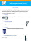
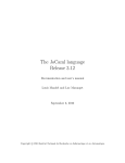
viscous_fluxes=’5p’, which is the most CPU efficient, may lead to unphysical results (see figure 2.1); viscous_fluxes=’3p’ is the less CPU efficient;
viscous_fluxes=’5p_cor’ is often a good compromise.
15
hopefully not oversimplified . . .
Ref.: /ELSA/MU-03037
Version.Edition : 1.1
Date : June 4, 2007
Page :
elsA
28 / 79
DSNA
User’s Starting Guide
THI Passot-Pouquet 32 x 32 x 32
Calcul LES à Reyt=74.
900
800
700
600
500
E(k) * 100
400
300
200
v3201d,
v3003p,
v3201d,
v3201d,
100
grad
grad
grad
grad
3p
3p
5p
5p cor
QPF elsA-LES Num. 2
5
CERFACS
10
15
k
Figure 2.1: Turbulent energy (THI computation)
.
elsA
DSNA
2.6.2
User’s Starting Guide
Ref.: /ELSA/MU-03037
Version.Edition : 1.1
Date : June 4, 2007
Page :
29 / 79
Time integration
The best time integration algorithms are different for steady and unsteady computations.
2.6.2.1
Local / Global time step
• Local time-stepping, where the time step is not constant across the computational domain, can be used in steady computations to speed overall convergence;
in that case, the user must choose the CFL number: high CFL values generally
increase convergence rate, but may lead to numerical instability.
• Conversely, in unsteady computations, where time accuracy is required, the user
must select a global time step: it must be small enough so as to resolve correctly
the unsteady phenomena, but not to small in order to minimize the number of
time steps.
2.6.2.2
Explicit stage
In the explicit stage, the time integration is based upon either a multi-stage RungeKutta algorithm, or a standard backward-Euler scheme.
2.6.2.3
Implicit stage
In both steady and unsteady cases, an implicit stage is generally added to speed up the
total computation time, by bypassing the time step limitation of explicit schemes. The
most widely used implicit operators are:
• Implicit Residual Smoothing (IRS); it is used in association with centered Jameson’s scheme, with Runge-Kutta 4-stage explicit time integration.
•
2.6.3
LU or LUSSOR : they may be used with both centered and upwind spatial discretization schemes, with backward Euler explicit time integration.
Multigrid acceleration
Multigrid uses a sequence of successively coarser meshes; in some cases, it can be a
very powerful tool to accelerate convergence. To use multigrid, users must provide
meshes which can be coarsened in each direction: if ng grid levels are desired, the
number of points of the fine grid must be divisible by 2ng + 1. In fact, the constraint
is even stronger: each boundary condition must be "coarsen-able". Also, a minimum
number of points must remain in the coarsest grid; this minimum depends on the spatial
discretization scheme:
• 3 nodes (2 cells) with Jameson’s scheme;
• 4 nodes (3 cells) with Upwind schemes.
Ref.: /ELSA/MU-03037
Version.Edition : 1.1
Date : June 4, 2007
Page :
2.6.4
elsA
30 / 79
User’s Starting Guide
DSNA
Other acceleration techniques
We do not discuss here either Low Speed Preconditioning or Dual Time Stepping.
Please consult the Theoretical Handbook and User’s Reference Manual.
2.6.5 Some useful examples
In the following, we shall try to provide a limited set of useful associations; starting
from these examples, it is hoped that users will tune the numerical parameters to their
specific problem in far less time than by starting from scratch. To keep examples as
compact as possible, we have used default values (see 5.1) in a systematic way.
2.6.5.1 Centered scheme, steady computation
May be used in subsonic/transonic configuration.
num = numerics(name=’num’)
# spatial discretization scheme
num.flux = ’jameson’
num.set(’avcoef_k2’, 0.5)
num.set(’avcoef_k4’, 0.032)
# temporal integration scheme
num.ode
= ’rk4’
num.implicit = ’irs’
num.cfl = 4.
# typical CFL number
2.6.5.2
Centered scheme, unsteady computation
num = numerics(name=’num’)
# spatial discretization scheme
num.flux = ’jameson’
num.set(’avcoef_k2’, 0.5)
num.set(’avcoef_k4’, 0.032)
# temporal integration scheme
num.time_algo = ’unsteady’
num.ode
= ’rk4’
num.implicit = ’irs’
num.timestep = ?
# global time step
num.itime
= ?
# simulation initial time
num.ftime
= ?
# simulation final time
2.6.5.3
Unsteady computation, dual time step (DTS)
num.set(’ode’, ’backwardeuler’)
num.set(’time_algo’, ’dts’)
num.set(’cfl’, 4.0)
num.set(’restoreach_cons’, 5.e-2)
num.set(’dual_iteration’, 50)
elsA
DSNA
2.6.5.4
User’s Starting Guide
Ref.: /ELSA/MU-03037
Version.Edition : 1.1
Date : June 4, 2007
Page :
31 / 79
Centered scheme, steady computation with multigrid acceleration
num = numerics()
# spatial discretization scheme
num.flux = ’jameson’
num.set(’avcoef_k2’, 0.5)
num.set(’avcoef_k4’, 0.032)
# temporal integration scheme
num.ode
= ’rk4’
num.implicit = ’irs’
num.multigrid = ?
num.coarse = ?
num.cfl = 4.
# typical CFL number
2.6.6
Upwind scheme, steady computation
May be used in subsonic/transonic, as well as in supersonic/hypersonic configuration.
num = numerics()
# spatial discretization scheme
num.flux = ’roe’
# Must be used with caution in viscous flow computation
# temporal integration scheme
num.ode
= ’backwardeuler’
num.implicit = ’lurelax’
num.cfl = 10.
2.7
Run the simulation
This is probably the easiest part:
problem.compute()
The current version allows users to chain several <cfdpb>.compute in the same
run 16 :
init1 = init(name=’init1’)
init1.file = ’restart_1’
cfd.compute()
cfd.reuse = ’active’
cfd.compute()
2.8
Information extraction
elsA users can be interested in lots of data, during and after a simulation. We will not
even try to explain all the extraction modes available. Here, our advice is: experiment
yourself, and read the User’s Reference Manual. Let us only give some examples.
16
Note however that in the current version, mesh sequencing runs cannot be chained in the same
script.
Ref.: /ELSA/MU-03037
Version.Edition : 1.1
Date : June 4, 2007
Page :
2.8.1
elsA
DSNA
User’s Starting Guide
32 / 79
Restart files
Restart files may be obtained with explicit creation of extractor objects:
e_restart = extractor(name=’e_restart)
e_restart.set(’var’, ’conservative’)
e_restart.set(’file’, ’restart’
e_restart.set(’loc’, ’cell’)
See section 3.1 for a faster and safer way to specify restart file management.
2.8.2
Convergence information
Convergence information can be sent both to standard output and to a file:
res_stdout
= extractor(name=’res_stdout’) # extraction on stdout
res_stdout.var = ’residual_ro’
# density residual (L1 and L2)
res_file = extractor(name=’res_file’)
res_file.var = ’residual_conservative’
res_file.file= ’residual.tp’
res_file.norm= NORM_L2
2.8.3
# extraction in a file
# extract residual for each conservat
Lift and Drag information
APROF-KL-Wl/APROF-KL-Wl.py
extract_lift = extractor(Some_Family, name=’extract_drag’)
extract_lift.set("format","fmt_tp")
extract_lift.set("var","convflux_rou convflux_row")
extract_lift.set("period",PERIOD_EXTRACT_LIFT)
extract_lift.set("loc", INTERFACE)
extract_lift.set("fluxcoeff",COEFL)
extract_drag = extractor(Some_Family, name=’extract_drag’)
extract_lift.set("format","fmt_tp")
extract_drag.set("var","diffflux_rou diffflux_row")
extract_drag.set("period",PERIOD_EXTRACT_DRAG)
extract_drag.set("loc", INTERFACE)
extract_drag.set("fluxcoeff",COEFD)
2.8.4
Flow analysis
Let us give an example where the mesh coordinates and the Mach number are saved in
a Tecplot file, thus allowing further analysis of the computation.
extract_mach
extract_mach.var
extract_mach.file
extract_mach.format
=
=
=
=
extractor(name=’extract_mach’)
’xyz mach’
’mach.tp’
’bin_tp’
elsA
DSNA
3.
User’s Starting Guide
Ref.: /ELSA/MU-03037
Version.Edition : 1.1
Date : June 4, 2007
Page :
33 / 79
MULTI-ZONE COMPUTATIONS
elsA accepts multi-zone structured meshes. Each zone corresponds to one (and only
one) mesh object. Each mesh is, in turn, attached to its corresponding block.
m1 = mesh()
m1.file’ = ’m1.tp’
m1.format = ’fmt_tp’
b1 = block()
b1.mesh = m1
m2 = mesh()
m2.file’ = ’m2.tp’
m2.format = ’fmt_tp’
b2 = block()
b2.mesh = m2
Note that a file is associated to a single zone: this is a very simple way to store mesh
data. For massively parallel configurations, it is probably the safest way to obtain
a fully scalable solution. However, for large configurations, the management of a
large number of files, and the definition of many objects in the script file (to specify
mesh and restart files) can become cumbersome. Future releases will provide access to
hierarchical CGNS data base file, where a single file can store the data corresponding to
every zone (and much more) 1 . In addition, elsA users can choose to let elsA generate
"internally", in an automatic and safe way, block, mesh, init and extract (for restart)
objects. This is described in the next section.
3.1
Automatic generation of block, mesh and init objects
To choose this mode, we must use the <cfdpb>.automatic_block_gen attribute. Mesh files, init files (if any) and restart files follow the same naming convention:
• they must belong to a single directory; for example, Mesh_d, Flow_i_d,
Flow_o_d for mesh, init and restart files, respectively.
• File names are built with a prefix, completed with digits: my_prefix000,
my_prefix001, ...
Most attributes admit default value (the exception is cfd_nb_block).
1
Note however that if a global file system is not available, which frequently happens for low-cost
cluster systems, a copy of the CGNS file must be available on all the computing nodes, which can be
cumbersome.
Ref.: /ELSA/MU-03037
Version.Edition : 1.1
Date : June 4, 2007
Page :
elsA
34 / 79
User’s Starting Guide
DSNA
naca = cfdpb(name=’naca’)
naca.set(’automatic_block_gen’,’db_directory)
naca.set(’cfd_nb_block’,2)
DEFAULT=1
# Optional parameters
if not DEFAULT:
naca.set(’cfd_block_prefix’,’Block’)
naca.set(’cfd_file_index0’, 0)
naca.set(’cfd_file_digit’,4)
naca.set(’cfd_mesh_format’,’fmt_tp’)
naca.set(’cfd_flow_out_format’,’fmt_tp’)
naca.set(’cfd_flow_ini_format’,’fmt_tp’)
#-------------------# MESH
#-------------------naca.set(’cfd_mesh__dir’,’Mesh’) # ’Mesh’ is actually default
#--------------------# Flow initialisation
#--------------------RESTART_FROM_FILE=1
if RESTART_FROM_FILE:
naca.set(’cfd_flow_ini_dir’,’Flow_ini’)
else:
naca.set(’cfd_init_state’, ’sta’)
#--------------------# restart file
#--------------------naca.set(’cfd_flow_out_dir’,’Flow_out’)
3.2
Zone connectivity
In principle, one can think of clever geometrical algorithms which would be able to
generate zone connectivity information when parts of a zone connect with parts of another zone or itself, without any additional user inputs. However, elsA use a different
strategy, for several reasons:
• Coding of such algorithms is certainly not an easy task; we are not sure that it is
even achievable in the most general case.
• Even in cases where such algorithms could be used, the associated cost may
not be negligible compared with CFD computations 2 . It is thus more efficient
2
Specially on vector computers, since these geometrical algorithms are not easily vectorisable.
Ref.: /ELSA/MU-03037
Version.Edition : 1.1
Date : June 4, 2007
Page :
elsA
DSNA
User’s Starting Guide
35 / 79
to store the connectivity information once, saving us the cost of re-computing
connectivity information at the beginning of every run.
There are three types of connectivity that can occur 3 : point-by-point, patched, and
over-set.
• The point-by-point, or 1-to-1, type occurs when the edges of zones abut, and
where grid vertices from one patch exactly correspond with grid vertices from
the other, with no points missing a partner.
• The patched type occurs when the edges of zones abut, but there is not a correspondence of the points, or they are not partnered with another point.
• The over-set type occurs when zones overlap one another (or a zone overlaps
itself). We do not describe mismatched (patched) or over-set connectivity information in this document: the user is referred to User’s Reference Manual for
details.
3.2.1 match: 1-to-1 connectivity definition
The easiest way to explain how to specify 1-to-1 connectivity is, as usual, to give a
simple example:
b1 = block(name=’b1’)
join1 = new_join(’join1’, ’b1’, ’join2’, f_match,
(23, 23, 1,7, 1,7))
b2 = block(name=’b2’)
join2 = new_join(’join2’, ’b2’, ’join1’, f_match,
( 1,
1, 1,7, 1,7))
In this example, the ’i=IMAX=23’ edge of block b1 abuts the ’i = 1’ edge of block
b2. f_match is a user-chosen arbitrary integer.
Internally, elsA uses an algorithm to find the orientation of the abutting faces. In some
cases, this algorithm fails, and users have to provide additional information, in the
form of an additional Python tuple (here (1,-2,3)):
join = new_join(’b1’, ’join2’, f_match,
(23, 23, 1,7, 1,7), (1,-2,3))
Remark : A good practice is to always explicitly give the orientation tuple.
3.2.2 near_match: 1-to-n connectivity definition
new_join_nearmatch(’b1E’,’b1’,’b2W’, Fam, (23,23, 1, 17, 1,17), ’fine’,
(2,2,2), (1,
new_join_nearmatch(’b2W’,’b2’,’b1E’, Fam, ( 1, 1, 1, 9, 1, 9), ’coarse’, (2,2,2), (1,
Compared with type=’match’, the only added information is a Python tuple (here
(2,2,2)) giving the refinement ratio.
3
Once again, readers are strongly advised to consult CGNS documentation, specially:
Overview and Entry-Level Document, Appendix C.
CGNS
Ref.: /ELSA/MU-03037
Version.Edition : 1.1
Date : June 4, 2007
Page :
3.2.3
elsA
36 / 79
User’s Starting Guide
DSNA
nomatch
g1 = globborder(name=’g1’)
g2 = globborder(name=’g2’)
new_join_nomatch(’Bnd0001’, ’Block0000’, ’g1’,’g2’, Fam, (23,23, 1,17, 1,17))
new_join_nomatch(’Bnd0006’ ’Block0001’, ’g2’,’g1’, Fam, ( 1, 1, 1,17, 1,17))
3.2.4
nomatch_linem
new_join_nomatch_linem(’Bnd0001’,
’Block0000’, ’g1’,’g2’, Fam, (23,23, 1,17, 1,17)
Compared with type=’nomatch’, the only added information is a Python tuple
(here (0,0)) giving the internal ordering inside the globborder "global reference
frame".
3.2.5 overlap
new_join(’Bnd0002’, ’Block0000’, ’overlap’, Fam, (10, 202, 1,1, 1,2))
elsA
DSNA
User’s Starting Guide
Ref.: /ELSA/MU-03037
Version.Edition : 1.1
Date : June 4, 2007
Page :
37 / 79
UNITS, DIMENSIONAL AND NON-DIMENSIONAL DATA
4.
To solve the Navier-Stokes (or Euler) equations, it is often convenient, although not
mandatory, to use dimensionless quantities. In some cases, using a well-chosen normalization can improve numerical accuracy 1 , specially inside geometric algorithms
(metrics computation, neighbour search (chimera) . . . ).
Let us recall that it is equivalent to say either that the quantity x is non-dimensionalised
referred to a length, L, or that the unit of length is chosen such that the length of x is
unity.
Contrary to many other scientific software, elsA do not use a specific unit system. This
means that users do not have to adapt to a unit system not suited to their needs. Of
course, this freedom has a price: it is up to the user to enter all values using a coherent
unit system.
Remark : An additional Python module, adim_lib, is available to help users in the choice of
a convenient normalisation system. See "Additional Tools User’s Manual", http://elsa.
onera.fr/ExternDocs/user/MU-06023.pdf, for a complete description.
4.0.6
Example: viscous coefficients
In viscous computations, since fluid molecular viscosity is computed with Sutherland’s
law :
r
T 1 + Cs /Ts
(4.1)
µ = µs
Ts 1 + Cs /T
the users must provide the 3 coefficients:
• suth_const : Cs constant in non-dimensional form (110.4/Tref ).
• suth_muref : µs , non-dimensional molecular viscosity corresponding to T =
Ts .
• suth_tref : Ts , non-dimensional temperature to define µs .
mod1 = model(name=’mod1’)
mod1.suth_const = 1.
mod1.suth_muref = 1.E-4
mod1.suth_tref = 1.0
All quantities must be given in accordance to the non-dimensional form chosen by the
user to the equations. The µs value fixes the Reynolds of the computation.
In turbulent computations with transport-equation models, users must additionally supply cutoffs values (section 6.3.1).
1
This is related to floating point arithmetic properties.
Ref.: /ELSA/MU-03037
Version.Edition : 1.1
Date : June 4, 2007
Page :
elsA
User’s Starting Guide
38 / 79
DSNA
For post-processing purpose, it is often useful to express the pressure coefficient and
the global aerodynamic forces with their usual definitions. In dimensional or nondimensional quantities in coherent unit system, we have :
Kp =
p − p∞
1
ρ U2
2 ∞ ∞
R
CF Σw =
=
p − p∞
1
p M2
2 ∞ ∞
flux dΣ
Σw
1
ρ U2 S
2 ∞ ∞
(4.2)
(4.3)
The quantity CF Σw may be any of the forces acting on a solid wall boundary. As the
integration of the fluxes is done over the boundaries, the reference surface S must be
chosen in agreement with the mesh definition. The flux integral is obtained using the
extraction of convflux_rou for the pressure forces in x-direction or diffflux_rou
for the friction forces in x-direction (see the User Manual).
In the following, we will discuss in some details five useful examples of
unit/normalization systems, and give some advice to avoid common errors, specially
for viscous computations.
4.1
SI
units
The user must enter every quantities using SI units: meter (length), kilogram (mass),
second (time), Kelvin (temperature), from which derived units can be built:
• velocity V : m/s;
• density ρ : kg/m−3 ;
• pressure P : Pa (kg m−1 s−2 );
• specific internal energy e: kg/m−1 s−2;
• viscosity coefficient µ : Poiseuille ( (Kg m−1 s−1 or N s m−2 )).
This system is very simple. However, a common error is to introduce mesh coordinates
in a non-SI unit (for instance, millimeters or centimeters).
4.2
Free-stream dimensioning: free-stream velocity scaling
In this system, a reference length, L, the free-stream density, ρ∞ , free-stream velocity,
U∞ , and free-stream temperature T∞ , are unity. This system is very popular, specially
in external flow computations. Every other fluid quantity is then non-dimensionalised
Ref.: /ELSA/MU-03037
Version.Edition : 1.1
Date : June 4, 2007
Page :
elsA
DSNA
User’s Starting Guide
39 / 79
using a reference quantity with the corresponding dimension. Introducing Mach number, M∞ = U∞ /a∞ (where a∞ is the free-stream speed of sound), and specific heat
ratio, γ (a2∞ = γP∞ /ρ∞ ), we obtain:
a∞ =
P∞ =
e∞ =
1
M∞
1
2
γM∞
1
= Cv
2
γ(γ − 1)M∞
P
1
=
2
ρT
γM∞
R=
where R is the gas constant (R = P/(ρT )), and Cv is the specific heat capacity
(e = CvT ).
In viscous computation, we also introduce the Reynolds number,
Re∞ =
ρ∞ U∞ L
µ∞
µ∞ =
Sutherland’s law:
r
µ = µs
1
Re∞
T 1 + Cs /Ts
Ts 1 + Cs /T
(4.4)
With REINF=Re∞ and TINFDIM=T∞ K, one have :
mod1 = model(name=’mod1’)
mod1.suth_const = 110.4/TINFDIM
mod1.suth_muref = 1./REINF
mod1.suth_tref = 1.0
4.3
Free-stream dimensioning: free-stream pressure scaling
This system is a slight variant of the previous one 2 . Here, the free-stream pressure
(instead of the free-stream velocity) is unity.
a∞ =
√
γ
√
U∞ = M∞ γ
2
often used in hypersonics computation
Ref.: /ELSA/MU-03037
Version.Edition : 1.1
Date : June 4, 2007
Page :
elsA
DSNA
User’s Starting Guide
40 / 79
e∞ =
1
(γ − 1)
R=1
1
γ−1
√
M∞ γ
ρ∞ U∞ L
=
=
Re∞
Re∞
Cv =
µ∞
The Sutherland law is expressed as in the previous case.
4.4
Stagnation condition dimensioning
In this system, the stagnation density ρi , the stagnation temperature Ti and the sound
velocity ai corresponding to Ti are taken equal to unity :
−1
γ−1 2
(4.5)
M∞
a∞ =
1+
2
u∞ = M∞ a∞
(4.6)
p∞
1
=
γ
−γ
p
γ − 1 2 γ−1
M∞
= 1+
pi ∞
2
(4.7)
ρ∞
1
=
γ
−1
γ − 1 2 γ−1
ρ
= 1+
M∞
ρi ∞
2
(4.8)
R=
p
1
=
ρT
γ
e∞ = Cv T∞
;
1
=
γ(γ − 1)
E∞ = Cv Ti =
ρ∞ U∞
µ∞
M∞ ρ
T
=
Re∞ ρi ∞ Ti ∞
Kp =
γp − (p/pi )∞
2
ρ∞ U∞
2pi
1
γ(γ − 1)
γ−1 2
1+
M∞
2
1
γ(γ − 1)
Re∞ =
µ∞
Cv =
(4.9)
−1
(4.10)
(4.11)
(4.12)
(4.13)
(4.14)
Ref.: /ELSA/MU-03037
Version.Edition : 1.1
Date : June 4, 2007
Page :
elsA
DSNA
4.5
User’s Starting Guide
41 / 79
Critical state dimensioning
In this system, the critical density ρc , the critical temperature Tc and the sound velocity ac corresponding to Tc are taken equal to unity :
a∞
1 + γ−1
2
=
2
M∞
1 + γ−1
2
(4.15)
u∞ = M∞ a∞
(4.16)
p∞
1 (p/pi )∞
1
=
=
γ (p/pi )c
γ
ρ∞
(ρ/ρi )∞
=
=
(ρ/ρi )c
R=
1
p
=
ρT
γ
e∞ = Cv T∞
µ∞
1 + γ−1
2
2
1 + γ−1
M∞
2
;
(4.17)
1
! γ−1
(4.18)
1
γ(γ − 1)
(4.19)
1 + γ−1
2
γ−1
2
1 + 2 M∞
!
γ+1
2γ(γ − 1)
(4.20)
(4.21)
(4.22)
1 + γ−1
2
2
1 + γ−1
M∞
2

4.6
γ
! γ−1
ρ∞ U∞
µ∞
M∞
=
Re∞
Kp =
Cv =
1
=
γ(γ − 1)
E∞ = Cv Ti =
Re∞ =
1 + γ−1
2
2
M∞
1 + γ−1
2
2 
p
2
M∞
1
1
! γ−1
1 + γ−1
2
2
+ γ−1
M∞
2
(4.23)
1
! γ−1

− 1
(4.24)
Turbulent conservative variables and cutoff
The choice of the boundary values to impose to the turbulent conservative variables and
to the corresponding cutoff is not trivial since it depends on the non-dimensionality and
of the turbulence models. However, the rule of thumb is relatively simple : the user
must choose the turbulence level Tu∞ of order 10−4 or 10−3 and the turbulent Reynolds
Ref.: /ELSA/MU-03037
Version.Edition : 1.1
Date : June 4, 2007
Page :
elsA
42 / 79
User’s Starting Guide
DSNA
number (µt /µ)∞ of order 10−2 . These quantities are only given for numerical purpose
and, in particular, Tu∞ has generally nothing to do with the turbulence level of a wind
tunnel to impose for transition criteria.
2
Tu2 /2 and the second turbulent quantity is
From the Tu definition, one have k∞ = 3U∞
obtained from µt /µ through the µt formulation of each particular turbulence model. To
simplify, one can take the wall damping function appearing in µt equal to unity Except
for the Wilcox model without Zheng limiter, the solution is normally insensitive to the
values at infinity providing they are small enough. One must not hesitate to check the
(µt /µ)∞ (var=’viscrapp’ quantity) issued from the computation.
4.7
Summary
Let us provide a Python script example, which may make the normalization task less
prone to user errors.
from math import *
# Some flow characteristics
MachInf = 9.86
Gamma
= 1.40
Reynolds = 1.E5
Alpha
= 0.
if FREESTREAM_NORM:
Pinf
= 1. / (Gamma*MachInf*MachInf)
RoInf
= 1.
RouInf = cos(Alpha)
RovInf = 0.
RowInf = sin(Alpha)
RoeInf = Pinf/(Gamma-1.) + 0.5
Cv
suth_const
suth_muref
suth_tref
= Pinf / (Gamma-1.)
= 110.4/TinfDim
= 1./Reynolds
= 1.
else if SI_UNIT:
Cv = 717.
R = 8.31
elsA
DSNA
User’s Starting Guide
5.
DEFAULT VALUE MECHANISM
5.1
Why default values?
Ref.: /ELSA/MU-03037
Version.Edition : 1.1
Date : June 4, 2007
Page :
43 / 79
In many cases, elsA tries to simplify the problem definition by providing default values. Let us give some examples.
• Assume that the user has not provided an explicit choice for the artificial viscosity. In that case, elsA provides a default value, currently artviscosity
=’dissca’.
num = numerics(name=’num’)
num.flux = ’jameson’
# flux type MUST be provided
# num.artviscosity = ’dissca’ # Note the ’#’: this line is a comment
• Here, the user does not define the data format associated with the extract
object. elsA provides fmt_tp as default value.
ext = extractor(name=’ext’)
ext.var = ’xyz mach’
ext.file = ’mach.tp’
# ext.format = ’fmt_tp’ # Note the ’#’: this line is a comment
Conversely, note that some values must be entered by users. For instance, users must
choose a flux type to associate with any numerics object. If they do not, elsA will
return some kind of error message (see also 5.2 and 9.2.3):
# elsA [2114] ERROR: User Error.
# info [2114] No Key flux
We are convinced that default values are very convenient for most users, and specially
for newcomers:
• elsA scripts can be more compact; the important feature of a given computation
are thus not "lost" in a very large script file.
• When a new option is added to the software, without a default value mechanism,
every already existing script would have to be modified, simply to say ’No, I do
not want to use this option’. Clearly, this is not acceptable.
• elsA default values are not hard-coded inside compiled code; instead, they are
stored in a "resource file" that can be customized to specific needs: in fact, this
resource file (see 5.2) can be modified by local elsA experts, so that less advanced users will benefit from their experience. For instance, one can imagine
that a computing site specialized in hypersonic flows may choose different default settings than a a computing site specialized in turbo-machinery computation.
Ref.: /ELSA/MU-03037
Version.Edition : 1.1
Date : June 4, 2007
Page :
elsA
User’s Starting Guide
44 / 79
DSNA
However, default values have their price:
• Some users definitely wish to see in a single script file the complete problem
definition; of course, these users are entirely free to avoid using any default
values.
• A bigger problem, in our opinion, is that experienced users may have the unpleasant feeling that they do not know exactly which options elsA has chosen
"behind the curtain". Two answers to this legitimate concern are given in the
next sections 1 .
5.2
What is the default value associated with a given attribute?
Internally, elsA default values are stored in a Python dictionary, dict_def_val ,
which can be consulted in Python module EpKernelDefVal.py 2 . For example,
running the following command 3 :
cat $ELSAHOME/Dist/lib/py/EpKernelDefVal.py
| grep ’\’format\’’
We obtain:
’format’
: ’fmt_tp’,
Another (better) way to get default value associated with any attribute is to issue the
following Python commands, either from the Python interpreter itself,
bash-2.03# python
...
>>> import EpKernelDefVal
>>> print EpKernelDefVal.dict_def_val[’format’]
fmt_tp
>>>
or from the elsA interpreter:
elsA(py) >>> import EpKernelDefVal
elsA(py) >>> print EpKernelDefVal.dict_def_val[’format’]
fmt_tp
elsA(py) >>>
So, you are now able to answer the question: "What is the default value associated with
a given attribute?". Another question is: "Do elsA provide a default value for a given
attribute?". As seen before (section 5.1), you can obtain an answer a posteriori, simply
by removing attribute definition from script and running the simulation. A cleaner way
is to run the same Python (or elsA) command:
1
The following section, 5.2 may be safely skipped by newcomers.
usually found in directory $ELSAHOME/Dist/lib/py
3
or grep ’"format"’ for older versions
2
elsA
DSNA
User’s Starting Guide
Ref.: /ELSA/MU-03037
Version.Edition : 1.1
Date : June 4, 2007
Page :
45 / 79
elsA(py) >>> import EpKernelDefVal
elsA(py) >>> print EpKernelDefVal.dict_def_val[’flux’]
Traceback (innermost last):
File "<console>", line 1, in ?
KeyError: flux
elsA(py) >>>
For additional information, consult User’s Reference Manual, specially
get_defaults, show_defaults, use_defaults, show_origin and
view.
Ref.: /ELSA/MU-03037
Version.Edition : 1.1
Date : June 4, 2007
Page :
elsA
46 / 79
User’s Starting Guide
DSNA
ADVANCED PROBLEM DEFINITION
6.
This chapter covers material not discussed in Chapter 2.
6.1
Family
It is often convenient to gather boundaries which share a common properties into
family objects:
• in this example, all the boundaries that are or type type=’walladia’ belongs to family F_WALL, where F_WALL is a pre-defined (positive) integer.
F_WALL=14
bnd1 = new_boundary(’bnd1’,’bk0’,’b_wall’, F_WALL,
...
bndn = new_boundary(’bndn’,’bkN’,’b_wall’, F_WALL,
(1, 1, j1, j2, k1, k2))
(1, 1, j1, j2, k1, k2))
• For more complex configurations, it can be useful to divide the "wall" family
into subsets, for example, when computing a complete aircraft, one family for
the wing, another one for the fuselage . . .
The power of the family concept appears when we have to define post-processing
(extraction), specially in parallel MPI: contrary to individual boundaries, which are not
invariant through block splitting arising during the load balancing algorithm, families
are conserved, so that defining extraction using family is much easier and less error
prone than using directly boundary (or associated window) objects (see also section
2.8.3):
ext_wing
= extractor(F_WING,
name=’ext_wing’)
...
ext_fuselage = extractor(F_FUSELAGE, name=’ext_fuselage_wing’)
...
Remark : The family concept can also be used with boundary objects instantiated with
direct call to boundary constructor 1 . In that case, one must use <boundary>.family:
Bnd0000 = boundary(’Block0000’,’E_W_Bnd0000’,’inj1’,name=’Bnd0000’)
E_W_Bnd0000.set(’wnd’, [1, 1, 1, 17, 1, 7])
Bnd0000.set(’family’, 6)
1 i.e.
not with call to construction method new_boundary
elsA
DSNA
6.2
User’s Starting Guide
Ref.: /ELSA/MU-03037
Version.Edition : 1.1
Date : June 4, 2007
Page :
47 / 79
Mesh sequencing
It frequently happens that we would like to perform computations with a coarsened
mesh:
• It may be convenient to perform preliminary computations on a coarsened mesh,
to find mistakes in the Python script(s), to identify any unforeseen problems, or
to tune numeric and physical parameters, without wasting too much resources.
• Comparing computations performed on coarse and fine mesh gives very useful
information concerning grid convergence. To achieve this, elsA provides users
with an easy to use, yet powerful, mechanism:
problem = cfdpb(name=’problem’)
problem.coarsen_mesh = 2
In this example, coarsening is uniform in the entire computational domain. Except this additional line 2 , the script is unchanged, which avoids many potential
errors.
• The total time to obtain converged results can sometimes be reduced through
several chained computations, converging first on the coarsest grid, using the
coarse solution to initialize solution on the finer grid (through any interpolation
algorithm), and going towards finest mesh. The idea is very similar to standard multigrid algorithm: long-wave perturbation are dissipated much faster on
coarse grids. Note that except for the coarsest level, if the coarsening factor
is equal to 2, it is possible to use multigrid acceleration: association of mesh
sequencing and multigrid is sometimes called Full Multi Grid (FMG).
To ease running FMG computations, elsA provides users with several attributes
(<cfdpb>.coarsen_mesh, <cfdpb>.coarsen_init, <cfdpb>.fromcoarse).
The following example shows how to chain three runs, going from coarse to fine grid
3
:
# 1st computation: 1 point over four
nozzle.set(’coarsen_mesh’, 4)
nozzle.set(’coarsen_init’, 4)
# Flow_0 contains some initialization for 1s1 mesh
nozzle.set(’cfd_flow_ini_dir’, ’Wksp/Flow_0’)
nozzle.set(’cfd_flow_out_dir’, ’Wksp/Flow_1s4’)
2
if initialization files are used (instead of initialization from constant state), a second line has to
been inserted:
problem.coarsen_init = 2
3
Consider using elsAsession in EpelsA.py to automate this process.
Ref.: /ELSA/MU-03037
Version.Edition : 1.1
Date : June 4, 2007
Page :
elsA
User’s Starting Guide
48 / 79
DSNA
num.set(’multigrid’, ’none’)
# 2nd computation: 1 point over two
nozzle.set(’coarsen_mesh’, 2)
nozzle.set(’fromcoarse’,
2)
nozzle.set(’cfd_flow_ini_dir’, ’Wksp/Flow_1s4’)
nozzle.set(’cfd_flow_out_dir’, ’Wksp/Flow_1s2’)
num.set(’multigrid’, ’v_cycle’)
num.set(’nbcoarsegrid’, 1)
# 3rd run
nozzle.set(’fromcoarse’,
2)
nozzle.set(’cfd_flow_ini_dir’, ’Wksp/Flow_1s2’)
nozzle.set(’cfd_flow_out_dir’, ’Wksp/Flow_1s1’)
num.set(’multigrid’, ’v_cycle’)
num.set(’nbcoarsegrid’, 2)
Presently, interpolation (prolongation) from coarse to fine grid use simple linear interpolation, without inter-block communications.
6.3
Numerical cutoffs
6.3.1
Cutoffs
Cutoffs are mainly used for the turbulent computation.
• muratiomax : maximum authorized value of µt /µ during a computation. This
cutoff may be needed for turbulence models in which the µt expression can
lead to 0/0. This is mainly the case for the k − ε model. This cutoff may be
used during the establishment phase of the solution and must be inactive when
convergence is reached. If this is not the case, the user does not use the expected
turbulence model but its own model! Depending on the Reynolds number, µt /µ
can take very different values. If the cutoff is set to 0, a laminar computation is
done.
• t_cutvar1 and t_cutvar2 : these cutoff on turbulent conservative variables are needed to avoid non physical negative values of these quantities. A
good practice is to define these cutoffs equal to a fraction (from 1. to 0.001 or
less) of the values at infinity (see paragraph 4.6).
elsA
DSNA
6.4
User’s Starting Guide
Ref.: /ELSA/MU-03037
Version.Edition : 1.1
Date : June 4, 2007
Page :
49 / 79
Topics not discussed
Many important subjects are still not covered in this document.
• Computations involving motions, in relative or absolute reference frame.
• Chimera computation. See (EVB):
validation/script/CHIM-2D-01/chim-2d-01.py
validation/script/RAE-KO-CHIM/rae-ko-chim-lam.py
• Transition.
• Data associated with boundary object in specific files, for instance to prescribe a
temperature field in isothermal wall boundary.
Ref.: /ELSA/MU-03037
Version.Edition : 1.1
Date : June 4, 2007
Page :
elsA
50 / 79
User’s Starting Guide
7.
ADDITIONAL INFORMATION
7.1
ICEM-CFD to elsA translator
DSNA
For complex multi-block configurations, writing manually elsA script files can be
cumbersome, and error-prone. Fortunately, users can use ICEM2elsA, a tool to automate the translation from ICEM - CFD topological files to elsA.
7.2
How to reduce start-up time?
For very large configurations, script files may be quite large. In most cases, this is
not a problem. However, on some platforms, specially vector computers (NEC, CRAY,
FUJITSU ), it has been observed that, in certain situations, the start-up time can be unbearable - more than ten minutes! Here are some guidelines to avoid such annoyance.
1. Use systematically the new_boundary / new_join syntax:
# preferred syntax
bnd = new_boundary(’bnd’, ’blk’, ’b_phys’, family, (i1, i2, j1, j2, k1, k2))
instead of the equivalent syntax with involves the creation of an auxiliary
window object:
# "Slow" syntax
win = window(’b’, name=’win’)
win.set(’iw1’, i1)
win.set(’iw2’, i2)
win.set(’jw1’, j1)
win.set(’jw2’, j2)
win.set(’kw1’, k1)
win.set(’kw2’, k2)
bnd = boundary(’blk’, ’win’, ’wallslip’, name=’bnd’)
2. As soon as your script is debugged, you can switch off most of the checks performed by the elsA interpreter, simply by adding the --fast option on the
command line1 :
elsa -f my_script.py --fast
This can reduce markedly the start-up time (typically by a factor of 2).
1
Caution : this option is incompatible with the "short" form, you have to use the set accessor.
elsA
DSNA
User’s Starting Guide
Ref.: /ELSA/MU-03037
Version.Edition : 1.1
Date : June 4, 2007
Page :
51 / 79
3. You can put all the invariant part of your script (and specially boundary condition definition) in a separate Python script file, say my_bnd.py. Python will
create a file my_bnd.pyc on the first interpretation; the .pyc files contain
”compiled” code, and are interpreted much faster in subsequent runs. Python
will automatically re-compile the original .py file if it is modified.
cfd = cfdpb(name=’cfd’)
...
import my_bnd # Please note : no extension!
...
4. Use the family concept to define post-processing, thus avoiding the trouble of
potentially extremely long lines 2 .
# preferred
Fuselage = 50 # Integer family code associated to fuselage part
bnd1 = new_boundary(..., Fuselage, ...)
bnd2 = new_boundary(..., Fuselage, ...)
...
ext = extractor(Fuselage), name=’ext’
ext.var = ’psta’
# deprecated
win1 = window(’blk’, name=’win1’)
win2 = window(’blk’, name=’win2’)
...
bnd1 = boundary(..., win1, ...)
bnd2 = boundary(..., win2, ...)
...
ext = extract_group(name=’ext’)
ext.windows = ’win1+win2+...’ # potentially very long string
7.3
Control of job execution
It is sometimes useful to be able to change the planned job execution during the run:
1. You receive a message from the system administrator:
System will be shut down in 5 minutes...
In such cases, you may wish to save the state of the computation, so that you can
start a new computation from this state, thus sparing precious computing time.
2. During a computation, you may wish to "see" dynamically if everything goes as
expected. Of course, you could have asked for periodic extractions by creating
extractor objects in the simulation script, in a static way. However, dynamic
interaction is definitely much more flexible.
2
Most text editors cannot manage properly lines exceeding a given limit.
Ref.: /ELSA/MU-03037
Version.Edition : 1.1
Date : June 4, 2007
Page :
elsA
52 / 79
User’s Starting Guide
DSNA
3. Your computation has been running for many hours, and you discover that you
have forgotten to ask for restart files in your script!
4. You may wish to change some computing parameters, for instance the CFL number. This is sometimes called Computational Steering; presently, elsA does not
provide such a facility.
The following two subsections (7.3.1 and 7.3.2) describe two mechanisms to deal with
the first three points.
7.3.1
Restart file
When elsA has entered the main (pseudo-) time loop, the user can ask that restart files
corresponding to the current iteration should be written. To do that, one must know
the Unix process number of the computing job (probably through the Unix command
ps). Then, the user must enter the following command 3 :
kill -SIGUSR2 <process_number>
Restart files will then be created; the file name will be constructed from the block
name and the time iteration: for instance, if blk1, blk2 are the names of the two
blocks in the problem, and the signal is sent during iteration 130, two files, named
blk1.iter00130 and blk2.iter00130 will be created. Then the process reenters the time loop, and the solution proceeds further on. Let us give an example of
the printed output, when the user has enter the kill command during iteration 18:
iteration no 17
----------------------------------------------------------------#dq 1 L2 = 4.3240937e-04 Linf = 9.0833416e-03 (
3 16 16 ) 0
#dq 2 L2 = 3.8816478e-04 Linf = 5.9381099e-03 (
3 16 16 ) 0
#dq 3 L2 = 2.3411757e-04 Linf = 4.1046026e-03 (
3 15 16 ) 0
#dq 4 L2 = 2.3411732e-04 Linf = 4.1046027e-03 (
3 16 15 ) 0
#dq 5 L2 = 1.1554889e-03 Linf = 2.8076357e-02 (
3 16 16 ) 0
----------------------------------------------------------------********************************************************************
iteration no 18
Dump restart file (process pid: 9044182, niter = 18)
....................................................................
elsA : Post-Processing for ’Block0000_pid0009044182_iter00018’
Write : Block0000_pid0009044182_iter00018
....................................................................
----------------------------------------------------------------#dq 1 L2 = 3.7224305e-04 Linf = 6.1108484e-03 (
4 16 16 ) 0
#dq 2 L2 = 3.5497200e-04 Linf = 5.6742947e-03 (
5 16 16 ) 0
3
On some platforms, you may have to replace SIGUSR2 by USR2 .
elsA
DSNA
User’s Starting Guide
Ref.: /ELSA/MU-03037
Version.Edition : 1.1
Date : June 4, 2007
Page :
53 / 79
#dq 3 L2 = 2.1372279e-04 Linf = 4.6443970e-03 (
3 15 16 ) 0
#dq 4 L2 = 2.1372277e-04 Linf = 4.6443970e-03 (
3 16 15 ) 0
#dq 5 L2 = 9.9448340e-04 Linf = 1.7954864e-02 (
3 16 16 ) 0
-----------------------------------------------------------------
7.3.2
SIGTSTP signal (Control-Z)
Another possibility to interact dynamically with a running job is to send it the
SIGTSTP signal. In interactive mode, you can use ’control-Z’ key combination. You
are then prompted with a menu:
Stop.......1
Extract....2
Continue...3
Kill.......4
1. The job is suspended:
[1] + Stopped (SIGSTOP)
/tools/Tempo/v2.2.10/Dist/bin/sgi/elsA.x x.py
Execution will continue if the user enters:
fg %1
2. The registered extract objects are scanned, and the corresponding files are
written: without the user interruption, these files would have been written at
the job’s end, during the job.extract() command. This option is specially
interesting to look at the convergence residuals. When all the extraction have
been performed, the user is prompted again with the same four possible choices
(Stop/Extract/Continue/Kill). Let us give an example, in which three
extractor objects have been registered:
********************************************************************
iteration no 7
----------------------------------------------------------------#dq 1 L2 = 2.1194850e-03 Linf = 2.5305340e-02 ( 16 16 16 ) 0
#dq 2 L2 = 1.9950121e-03 Linf = 2.0783402e-02 ( 17 16 16 ) 0
#dq 3 L2 = 1
Pause......1
Extract....2
Continue...3
Kill.......4
: 2
----------------------------------------------------------------#dq 1 L2 = 1.7171855e-03 Linf = 2.3111593e-02 (
7 16 16 ) 0
#dq 2 L2 = 1.4053604e-03 Linf = 1.4030115e-02 ( 15 16 16 ) 0
Ref.: /ELSA/MU-03037
Version.Edition : 1.1
Date : June 4, 2007
Page :
elsA
54 / 79
User’s Starting Guide
DSNA
#dq 3 L2 = 8.9873227e-04 Linf = 7.0547847e-03 (
5 15 16 ) 0
#dq 4 L2 = 8.9873191e-04 Linf = 7.0547845e-03 (
5 16 15 ) 0
#dq 5 L2 = 4.5892234e-03 Linf = 6.6441164e-02 (
7 16 16 ) 0
------------------------------------------------------------------....................................................................
elsA : Post-Processing for ’debam_1s1’
Write : debam_1s1
....................................................................
....................................................................
elsA : Post-Processing for ’debav_1s1’
Write : debav_1s1
....................................................................
....................................................................
elsA : Post-Processing for ’Wksp/Flow_1s1/flow0000’
Write : Wksp/Flow_1s1/flow0000
....................................................................
Pause......1
Extract....2
Continue...3
Kill.......4
: 3
********************************************************************
iteration no 9
...
3. Execution continues.
4. The job is killed immediately.
7.4
Script files and new releases
For each elsA release, the Python–elsA interface defines all the documented features
coherently with the User’s Reference Manual (URM), /ELSA/MU-98057 attached to
this release.
The URM details the various debugging procedures, including dealing with
Python–elsA scripts which are no more coherent with the current release (or conversely
using current scripts with older releases, if need be).
A global means of interface definitions comparison between two elsA versions is to
invoke, for each version, the man() function as :
man(’elsA’)
and to re-direct the output to a file.
Ex. :
<using ‘‘old’’ environment>
elsa --pycmds "man(’elsA’) ; close()" > old.out
<using ‘‘new’’ environment>
elsA
DSNA
User’s Starting Guide
Ref.: /ELSA/MU-03037
Version.Edition : 1.1
Date : June 4, 2007
Page :
55 / 79
elsa --pycmds "man(’elsA’) ; close()" > new.out
diff old.out new.out | more
For a given script, the following command-line options (definitions extracted from the
URM ) may be useful (please mind that option order is significant) :
--validate
--strict
--warn
--allow_obsolete
: check script coherency (see --warn below)
implies --noexecution --check --noraise --nowarn
--noshow --nostats
disables --allow_obsolete
keeps a memory of all errors (not final state only)
: warnings are treated as errors
: (re-)enable warnings (useful after --validate)
: accept automatic replacement of obsolete features
So that --validate --warn will check a script (not performing the computation)
with all warnings enabled, while --validate --strict will also perform only
a check, but treating warnings as errors.
Using --strict , specified without --validate , will abort the computation only
if any error or warning was found during the global check.
Remark : The --allow_obsolete option should not be used after --validate , because it defeats the purpose of catching inadequate specifications ; also, it is only meant to be
an aid in performing computations with old scripts, but may not perform all necessary conversions in all cases.
Ref.: /ELSA/MU-03037
Version.Edition : 1.1
Date : June 4, 2007
Page :
8.
elsA
56 / 79
User’s Starting Guide
DSNA
PARALLEL MODE
elsA implements coarse-grained block-based parallelism, based on MPI 1 . It is the
user’s responsibility to allocate blocks on each processor. Depending on the number of
processor and the individual block sizes, achieving good load balancing may require
that some blocks have to be split in several sub-blocks. Presently, this task must be
done by users before actually submitting their parallel job to elsA. Let us give a simple
example.
Before splitting:
-----------------------------------------|
|
b0
|
b1
|
|
|
-----------------------------------------|
|
|
b2
|
|
|
-----------------------------------------|
|
|
After splitting:
-----------------------------------------|
|
b0
|
b1
|
|
|
-----------------------------------------|
|
|
|
b20
|
b21
|
|
|
|
-----------------------------------------|
|
|
Once this pre-processing step is over, using elsA in
ward:
MPI
parallel mode is straightfor-
1. Script files are nearly identical in serial and parallel mode; the only additional
data to be specified is the mapping of blocks to processors. Two options are
available to define this mapping:
(a) use of attribute <block>.proc, that must be set for block 2 .
blk0 = block(name=’blk0’)
blk0.node = 0
blk1 = block(name=’blk1’)
blk1.node = 1
1
Future elsA releases may provide in addition OpenMP shared memory parallel processing
(OpenMP is the de facto standard for directive-based shared memory parallel processing); although
some experiments have already been done to parallelize elsA with OpenMP, OpenMP version is still
not officially supported.
2
And not for mesh or extract objects.
elsA
DSNA
User’s Starting Guide
Ref.: /ELSA/MU-03037
Version.Edition : 1.1
Date : June 4, 2007
Page :
57 / 79
(b) use of attribute <cfdpb>.mpi_block2proc:
my_cfdpb.set(’mpi_block2proc’, ’script_load_balance’)
Here, script_load_balance.py is a very simple Python script, containing a Python dictionary providing the mapping of blocks to processors.
The dictionary keys and associated values are the block numbers and the
processor numbers.
cat script_load_balance.py
# Splitted configuration : 5 blocks
# Number of processors
: 4
nproc = 1
dict_block2proc = {
0 : 0,
1 : 1,
2 : 1,
3 : 2,
4 : 3
}
2. At run time, launching elsA MPI executable is platform dependent; in many
situations, the following will work:
mpirun -np <nb_of_Proc> parallel_script.py
Ref.: /ELSA/MU-03037
Version.Edition : 1.1
Date : June 4, 2007
Page :
elsA
58 / 79
DSNA
User’s Starting Guide
TROUBLESHOOTING
9.
Since elsA is a complex system, user errors are unavoidable. Also, unfortunately,
internal errors may arise inside elsA kernel. This chapter presents the basics of error
treatment provided by elsA: it is hoped that a careful classification of error messages,
as well as a description of the most frequent ones, will help users to understand by
themselves what is going wrong, thus saving a lot of precious time.
It is useful to classify errors in three broad categories:
1. environment errors ;
2. interface errors ;
3. kernel errors.
9.1
Environment error
Let us give examples of errors resulting from incorrect environment; this should help
you to recognize what’s going on 1 . In case of trouble, please look carefully the first
few lines printed on the standard output after you enter the elsa command with -v
option:
$ elsa -v
elsA interface : Message : displaying (selected) control parameters :
verbose=echo use_import=off
platform nickname
= GNU/Linux
ELSAPROD
= intelIA32em
ELSAHOME
= /tmp_user/eos010/gazaix/v3301
ELSA_EXE
= /tmp_user/eos010/gazaix/v3301/Dist/bin/intelIA32em/elsA.x
PYTHONPATH
= /tmp_user/eos010/gazaix/v3301/Dist/lib/py
LD_LIBRARY_PATH
= /opt/intel/fce/9.0/lib:/opt/intel/cce/9.0/lib
9.1.1
Incorrect PYTHONPATH
Traceback (innermost last):
File "<string>", line 1, in ?
ImportError: No module named EpelsA_loader
9.1.2
Incorrect LD_LIBRARY_PATH
An example of message
LD_LIBRARY_PATH:
1
issued
by
Unix
system
with
an
incorrect
Depending on your platform and the version used, messages may be somewhat different.
elsA
DSNA
User’s Starting Guide
Ref.: /ELSA/MU-03037
Version.Edition : 1.1
Date : June 4, 2007
Page :
59 / 79
12700720:/tools/Tempo/v2.2.10/Dist/bin/sgi/elsA.x:
rld: Fatal Error: Cannot map soname ’libeDescp.so’ under any of:
/tools/gnome/lib/libeDescp.so:/usr/lib64/libeDescp.so
Check carefully your spelling: did you define LD_LIBARY_PATH?
9.1.3
Incorrect PYTHONHOME
Example of message written by the Python interpreter:
Could not find platform independent libraries <prefix>
Could not find platform dependent libraries <exec_prefix>
Consider setting $PYTHONHOME to <prefix>[:<exec_prefix>]
’import exceptions’ failed; use -v for traceback
Warning! Falling back to string-based exceptions
’import site’ failed; use -v for traceback
See 1.5 for a possible value of PYTHONHOME.
9.2
Interface errors
Users interact with the computational CFD kernel through a software layer, which we
will call here the elsA interface. The interface is written itself in Python; one can
view this layer as a "wrapper", providing users with a high-level CFD interpreter. The
interface layer provides many convenient mechanisms to check user inputs as soon as
possible, and so to be able to give users reliable information, and even in some cases
suggestions to correct the error (see also 7.4, p. 54). See User’s Reference Manual
for complete information. The interface cannot identify all the possible errors that
can arise during a computation. This may happen because of incomplete coherence
checks, or because of truly internal errors, such as failure of numerical algorithm: in
such cases, it will be the kernel’s job to implement the error treatment (see 9.3.1).
9.2.1
Syntax error
As in any language, users may enter invalid commands. Since the elsA interpreter is
built on top of Python, most syntax errors are reported by the Python interpreter itself
2
:
elsA(py) >>> mmm =
File "<console>", line 1
mmm =
^
SyntaxError: invalid syntax
2
in fact, this is one of the many advantages brought by extending an existing interpreter, instead of
writing yet another one by ourselves
Ref.: /ELSA/MU-03037
Version.Edition : 1.1
Date : June 4, 2007
Page :
9.2.2
elsA
60 / 79
User’s Starting Guide
DSNA
Invalid attribute
9.2.2.1
Unknown attribute
The user tries to give a value to an attribute which does not exist in the class to which
belongs the object ( in the following example, note the spurious ’h’ in gahmma):
elsA(py) >>> mod1 = model(name=’mod1’)
elsA(py) >>> mod1.gahmma = 1.4
# Note the spurious ’h’
elsA interface : ERROR : Name error :
unknown (macro-)attribute ‘gahmma’ for class ‘model’
(macro-)attribute name should be in :
[’baldwin_model’, ’constke’, ’constke1’, ’constke2’, ’constke3’, ’constke4’,
’cv’, ’fluid’, ’gamma’, ’michel_model’, ’models’, ’phymod’, ’phys_props’,
’prandtl’, ’prandtltb’, ’specrad_s_mean’, ’sst_cor’, ’suth_const’,
’suth_muref’, ’suth_tref’, ’tblx_ckleb’, ’tblx_distlim’, ’tblx_ibalditx’,
’tblx_preslim’, ’tblx_vortrlim’, ’tmic_cfg’, ’tmic_ctipleak’, ’tmic_delta’,
’tmic_deltamx’, ’tmic_itpf’, ’tmic_vortcrit’, ’tmic_vortlim’, ’tmic_vortrlim’,
’turbmod’, ’turbmod_variants’, ’type_asm’, ’type_keps’, ’visclaw’,
’viscosity’, ’walldistcompute’, ’zhenglim’]
... message is : unknown attribute ‘gahmma’ for class ‘model’
9.2.2.2 Invalid type
Here, the attribute exists, but the type of the associated value is wrong:
>>>
>>>
>>>
>>>
from elsA_user import *
cfd1 = cfdpb(name=’cfd1’)
mod1 = model(name=’mod1’)
mod1.set(’gamma’, 1)
elsA interface : ERROR
: Type error : wrong type for value : 1
... types : <type ’int’> vs <type ’float’>
... for ’gamma’ attribute of <model instance ’mod1’>
9.2.2.3
Invalid range
elsA(py) >>> mod1.gamma=-.5
elsA interface : ERROR : Value error : wrong value ‘-0.5’
for attribute ‘gamma’ of object : <model instance ’mod1’>
value(s) should be in :
]0,...,inf[
9.2.3
Attribute value required
A value is required but the user did not provide one and no default value exists : elsA
raises an error.
elsA
DSNA
User’s Starting Guide
Ref.: /ELSA/MU-03037
Version.Edition : 1.1
Date : June 4, 2007
Page :
61 / 79
# elsA [2114] ERROR: User Error.
# info [2114] No Key flux
Note that the previous message is provided at runtime by elsA kernel, not the (Python)
interface on a check() call.
Useful information about default value can also be obtained through check() :
elsA >>> num1 = numerics(name=’num1’)
elsA >>> num1.check()
elsA interface : Warning : using default value 2.9387360491e-39
for num1.convergence_level
... static default value, context-dependent one failed
elsA interface : Warning : using default value
’none’
... static default value, context-dependent one failed
elsA interface : Warning : using default value
’none’
... static default value
elsA interface : Warning : using default value
’none’
... static default value, context-dependent one failed
elsA interface : Warning : using default value
’rk4’
... static default value, context-dependent one failed
elsA interface : Warning : using default value
’steady’
... static default value, context-dependent one failed
elsA interface : Warning : using default value
’none’
... static default value, context-dependent one failed
for num1.multigrid
for num1.precond
for num1.artviscosity
for num1.ode
for num1.time_algo
for num1.implicit
elsA interface : ERROR
: Coherency error : missing value for num1.flux
... and no default value found or allowed for <numerics>.flux attribute
... <numerics>.flux attribute value is always required
9.3
Kernel errors
The separation between interface and kernel errors is not absolute. Being pragmatic,
we may define kernel errors as "every error which is not an interface error"! In fact, it
is not an easy task to design a clean error system, because the elsA kernel is used in
two different contexts :
• it is used through the elsA interface by elsA end users to perform
tations;
CFD
compu-
• it provides CFD scientists with a powerful Object-Oriented CFD toolkit 3 : they
can build their specific applications by combining kernel classes, deriving new
classes from existing ones, and adding their own classes. In this context, error
messages are sent to programmers, not to end users. We acknowledge that such
kernel error messages, intended for programmers, can be quite intimidating for
end users. Let us give an example:
3
an OO toolkit is equivalent to a Unix library.
Ref.: /ELSA/MU-03037
Version.Edition : 1.1
Date : June 4, 2007
Page :
elsA
62 / 79
User’s Starting Guide
DSNA
# elsA : Internal Error
Please check your script file,
and look carefully to warning/errors;
Then, Please submit a full bug report.
See <URL:http://elsa.onera.fr/elsA/query/PRsub.html>
# elsA [ File : .Obj/sgi/Base/BlkMesh.C (line no : 951)]
# elsA [9920] FATAL: Internal Error.
The "philosophy" corresponding to these two contexts is quite different : to be useful,
the toolkit must be very extensible, letting programmers do numerical experiments, at
their own risk. On the contrary, end users, and specially newcomers, must be provided
with as much safety guards as possible. Let us hope that a good compromise can be
found between these two conflicting requirements.
9.3.1
The three kernel error levels
Kernel errors are classified in three categories, according to the error severity :
1. WARNING: there is some inconsistency in the user input; elsA tries to do its best
to continue. Example 1:
E_ERRENTRY(2232, E_WARNING, "Rotation with null angle.",
"JoinBaseP.C", "No text")
Example 2: Boundary interface re-defined
# elsA [2350] ERROR: User Error.
# info [2350] Boundary Interface already defined :
blk1 : bnd111 : 1 1 2 3 1 2
........................................
2. ERROR: an error is detected. Processing continues, but garbage will almost
surely being produced. Example: Boundary interface not defined
# elsA [2361] ERROR: User Error.
# info [2361] Boundary Interface never defined :
blk : 69 69 63 64 1 2
........................................
3. FATAL: There is no way to continue: processing immediately stops. Example:
failure of memory allocation
Dynamic memory allocation algorithm has failed.
Please try increasing the process datasize limit
(ulimit in ksh, limit in csh).
If submitted with qsub, check ’-lm’ argument.
Note that the problem you try to solve may be too big for your machine...
elsA
DSNA
User’s Starting Guide
Ref.: /ELSA/MU-03037
Version.Edition : 1.1
Date : June 4, 2007
Page :
63 / 79
Detailed Memory Information:
Process asked for 1345294332 bytes
Current Total
count = 1345298532
-------------------------------------------------------------------------------# elsA [9110] FATAL: Out of Memory
Leaving error, code is 9110
# elsA : exit forced
9.4
Parallel errors
In MPI parallel mode, if something goes wrong, look carefully to each
logfile produced by each processor (elsA_MPI_Pid_xxxxxxx_N_0,
elsA_MPI_Pid_xxxxxxx_N_1 . . . ), paying special attention to any error
messages.
It is sometimes useful to run in sequential mode: in this case 4 , proc is simply ignored,
so that it is not necessary to remove definition of proc attributes. If the configuration
is too big to be run on a single processor, consider using <cfdpb>.coarsen_mesh
and <cfdpb>.coarsen_init 5 .
9.5
Stack overflow
In some rare cases, elsA might fail at runtime (probably with a "segmentation violation") due to overflowing the stack. Try to increase the stack size (typically using
limit stacksize (in csh and derivatives) or ulimit -s (in sh and derivatives).
9.6
What should you do in case of trouble?
9.6.1
Do not ignore warning messages
Warning / Error messages often provide a clue that something is going wrong. Please,
do not ignore them. Also, please read carefully log messages printed on stdout and
stderr. Look with special care the banner which is printed at the beginning of each
run; many information are provided, which can help you to perform many checks:
• elsA release, production date and mode:
#
#
#
#
#
4
5
elsA v3.1.06 - Copyright (c) 1997-2003 by ONERA
Production: Linux_japhet_2.2.13 - linux - Feb_16,_2002_-_16:44:08
C++ Compiler Option: -Wall_-march=i686_-mcpu=i686_-O_-DNDEBUG_-D_E_FORTRAN_LOOP
Fortran Compiler Option: -O_-Wall_-O3_-march=i686_-mcpu=i686
either running elsA sequential executable, or the parallel one, with N P ROC = 1
This is usable only if the configuration allows multigrid.
Ref.: /ELSA/MU-03037
Version.Edition : 1.1
Date : June 4, 2007
Page :
elsA
64 / 79
User’s Starting Guide
DSNA
• Information about single/double precision:
Size of Float
: 4 Bytes
Size of Integer : 4 Bytes
9.6.1.1
Special case: parallel mode
In parallel mode, each computing node writes to standard output its own messages.
Unfortunately, on some platforms, one can obtain scrambled outputs, quite difficult to
interpret. Future versions will avoid this annoying behaviour.
9.6.2
Some of the most frequent errors
Frequent user errors have already been discussed in section 9.2.1, 9.2.2, 9.2.3, 9.2.3.
Let us describe other common errors.
9.6.2.1
Use of reserved keywords
elsA scripts are really just Python scripts: so they must respect Python naming rules 6 .
Moreover, A limited set of keywords are used by the elsA interpreter 7 : it is forbidden
to name user-created objects with these keywords.
List of reserved elsA keywords:
cfdpb, mesh, block, numerics, model, init, extractor,
extract, extract_group, boundary, group, family, window,
globwindow, globborder.
Python has also its own list of reserved keywords, for example: if, else, ....
9.6.2.2 Duplicated object name
In order to distinguish between objects created by users, it is strictly forbidden to use
the same name for two objects, even if they belong to different classes.
w1 = window()
...
w1 = window()
Error : duplicated object name!
The duplicated name is : w1
You must choose non-ambiguous object name.
Sorry -- cannot continue.
# elsA [2111] FATAL: User Error.
6
7
For example, an identifier must not contain a . (dot) character.
These names are injected in the current scope through the from elsA_user import *.
elsA
DSNA
9.6.2.3
User’s Starting Guide
Ref.: /ELSA/MU-03037
Version.Edition : 1.1
Date : June 4, 2007
Page :
65 / 79
Memory problem
If you run out of memory, it is sometimes possible to increase the memory allowed by
the (Unix) system:
# give maximum size of data segment or heap (in kbytes)
ulimit -d
3906250
You may try:
ulimit -d unlimited
9.6.2.4
Arithmetic exception: NaN (Not a Number)
When a floating point exception is encountered, depending on the production, two
cases are possible:
• Computation stops immediately;
• Computation continues, until the next occurrence of convergence residual computation 8 .
Suggestion: it may help to reduce CFL, maybe starting from a relatively low value, and
increasing towards larger values :
f_cfl = function(’linear’)
f_cfl.set(’linear’,[2., 30.0, 500, 3000])
num.attach(f_cfl)
9.6.2.5
Turbulence does not develop
In case of Navier-Stokes computation with transport equation models, check that the
turbulence develops correctly. To this end, look at the residual of ρk. It must increase at the beginning of the computation. Use <init>.coeffmutinit and
iter_ini_tur if needed, in particular for Spalart-Allmaras and k − ε.
9.6.2.6
File error
Mesh m1 : file =’very_bidulic_file_name’
m1 : format=’fmt_tp’
# elsA [4011] FATAL: Fortran OPEN error
Suggestion: check file name and file permission. Please note that elsA is currently too
"laxist" about file ownership and permission; some checks should be added (so that,
for instance, re-start files cannot be inadvertently overwritten).
8
elsA test the residuals: if a NaN is found, computation is stopped.
Ref.: /ELSA/MU-03037
Version.Edition : 1.1
Date : June 4, 2007
Page :
9.6.3
elsA
66 / 79
User’s Starting Guide
DSNA
When all else fails
• Look at known bugs in the appropriate section of the elsA Web site
(http://elsa.onera.fr/elsA/use/refbugs.html).
• Search for interface changes, also in the appropriate section of the elsA Web site.
It may happen that some attributes have been changed, so that your python script
does not mean what you think. Look carefully to EpAttrDefs.py, and/or use
the man and check 9 interface commands:
elsA >>> man(’vel_formulation’)
Attribute name : vel_formulation
Class(es)
: numerics
Description
: velocity formulation for mobile grids
Allowed values : ’relative’, ’absolute’
Default value(s) : ’absolute’
Rules
:
dependency rules :
vel_formulation is meaningful only IF :
block.motion = ’mobile’
• Send an e-mail to [email protected].
See http://elsa.onera.fr/elsA/query/PRsub.html.
9
man(’elsA’) prints synthetic information for each attribute
elsA
DSNA
User’s Starting Guide
10.
FREQUENTLY ASKED QUESTIONS
10.1
How to convert elsA files from a format to another one
Ref.: /ELSA/MU-03037
Version.Edition : 1.1
Date : June 4, 2007
Page :
67 / 79
It occurs frequently that one has to convert a file from a given format, say formatted
Tecplot to another one, say binary VOIR 3 D. Instead of writing a conversion utility, it
is much better to let elsA do the work for us:
my_cfdpb = cfdpb(name=’my_cfdpb’)
m
m.file
m.format
...
blk
blk.mesh
...
e
e.var
e.file
e.format
e.loc
= mesh(name=’m’)
= ’m.tp’
= ’fmt_tp’
= block(name=’blk’)
= m
=
=
=
=
=
extractor(’blk’, name=’e’)
’xyz’
’m.v3d’
’bin_v3d’
’node’
num
= numerics()
num.iter = 0
# 0 iteration : no actual computation
my_cfdpb.compute()
my_cfdpb.extract()
Using automatic_block_gen=’db_directory’, the whole configuration
can be converted very easily:
my_cfdpb = cfdpb(name=’my_cfdpb’)
my_cfdpb.set(’cfd_mesh_format’, ’fmt_tp’)
...
# extractor without additional argument
# --> Applies to the whole configuration
e
= extractor(name=’e’)
e.var
= ’xyz’
e.file
= ’m.v3d’
e.loc
= ’node’
num
= numerics()
num.iter = 0
# 0 iteration : no actual computation
my_cfdpb.compute()
my_cfdpb.extract()
Ref.: /ELSA/MU-03037
Version.Edition : 1.1
Date : June 4, 2007
Page :
elsA
User’s Starting Guide
68 / 79
DSNA
At run time, for each block, a mesh file with format=’bin_v3d’ will be created:
m.v3d0000, m.v3d0001 ....
A similar trick can be used to extract a coarsened grid from the fine one:
m
m.file
m.coarse_i
m.coarse_j
m.coarse_k
...
e
=
e.var
=
e.file
=
e.loc
=
=
=
=
=
=
mesh()
’m_fine’
2
3
1
extractor(name=’e’)
’xyz’
’m_coarse’
’node’
This will create a file corresponding to a mesh with one point over two in the i direction,
one over three in j, and every point in k.
10.2
Can I exchange
forms?
VOIR 3 D
binary files between different computing plat-
The answer is YES; this is done through <cfdpb>.set_binv3d; see elsA User’s
Reference Manual for a complete discussion. For instance, binary files created by
elsA executables on COMPAQ (DEC - ALPHA) machines can be used by SGI, PC running
Linux 1 , and NEC computers.
Binary Tecplot files can be exchanged freely; note however that Tecplot binary files
are not available on all platforms.
1
An experimental version of elsA is available for PC running Windows ; this version requires that
Cygwin has been installed.
elsA
DSNA
Appendix A.
User’s Starting Guide
Ref.: /ELSA/MU-03037
Version.Edition : 1.1
Date : June 4, 2007
Page :
69 / 79
FORTRAN EXAMPLE CREATING A TECPLOT
MESH FILE
C
C
PROGRAM WRITE_GRID_TP
IMPLICIT NONE
INTEGER UNIT
INTEGER IMAX, JMAX, KMAX
INTEGER i,j,k
CHARACTER*8 cform
PARAMETER (UNIT=10)
PARAMETER (IMAX=12, JMAX=7, KMAX=7)
REAL x(IMAX,JMAX,KMAX), y(IMAX,JMAX,KMAX),z(IMAX,JMAX,KMAX)
Create Grid Points
DO i=1,IMAX
DO j=1,JMAX
DO k=1,KMAX
x(i,j,k) = float(i-1)
y(i,j,k) = float(j-1)
z(i,j,k) = float(k-1)
END DO
END DO
END DO
cform = ’(6E15.7)’
OPEN(UNIT, FILE=’./m1.tp’)
See Tecplot User’s Guide
WRITE(UNIT,’A’) ’TITLE = "First mesh example"’
WRITE(UNIT,’A’) ’VARIABLES = "x" "y" "z"’
WRITE(UNIT,’A’) ’ZONE T="grid 1 ", I=12, J=7, K=7, F=BLOCK’
WRITE(UNIT,cform) (((x(i,j,k), i=1,IMAX),j=1,JMAX),k=1,KMAX)
WRITE(UNIT,cform) (((y(i,j,k), i=1,IMAX),j=1,JMAX),k=1,KMAX)
WRITE(UNIT,cform) (((z(i,j,k), i=1,IMAX),j=1,JMAX),k=1,KMAX)
CLOSE(UNIT)
END
Ref.: /ELSA/MU-03037
Version.Edition : 1.1
Date : June 4, 2007
Page :
Appendix B.
B.1
CPU
elsA
70 / 79
User’s Starting Guide
DSNA
HOW TO RUN BENCHMARKS
efficiency
It is sometimes useful to know elsA CPU efficiency on a given platform 1 . A convenient
way to measure CPU efficiency is to divide the total CPU time by the time iterations and
the number of mesh points. The computed value will of course depend somewhat upon
the specific test case; however, if the problem size is large enough, since the cost associated with boundary treatment can be neglected, the efficiency will be nearly entirely
determined by the numerical scheme (spatial discretization and temporal integration).
To give an easy way to measure elsA performance, with complete freedom to specify
the number of blocks, and the number of mesh points inside each block, we have
provided an "automatic" way to build mesh objects, without the burden to create new
mesh files each time the problem size changes:
#
#
#
#
Example of automatic cartesian mesh generation
(avoid use of external mesh files)
2 block configuration
This script can be used to run \sigle{MPI} benchmark, with 2 computing nodes
from elsA_user import *
bench = cfdpb(name=’bench’)
cartesian_delta = 1. # Cell size
# Parallelepiped size
IM = 25
JM = 10
KM = 5
NPOINT = 2 * IM*JM*KM
# MESH CREATION
m0 = mesh(name=’m0’)
m0.set(’generator’, ’cartesian’)
m0.set(’im’, IM)
m0.set(’jm’, JM)
m0.set(’km’, KM)
m1 = mesh(name=’m1’)
m1.set(’generator’, ’cartesian’)
m1.set(’im’, IM)
m1.set(’jm’, JM)
m1.set(’km’, KM)
1
We may have to compare elsA with other CFD codes, or we have to check the efficiency of a a new
implementation (for example, quality of vectorization).
elsA
DSNA
User’s Starting Guide
Ref.: /ELSA/MU-03037
Version.Edition : 1.1
Date : June 4, 2007
Page :
71 / 79
# Offset of mesh 2
m1.set(’cartesian_orig_x’, (IM-1)*cartesian_delta)
# BLOCK CREATION
b0 = block(name=’b0’)
b0.set(’mesh’, ’m0’)
b0.set(’proc’, 0)
b1 = block(name=’b1’)
b1.set(’mesh’, ’m1’)
b1.set(’proc’, 1)
...
import time
t1=time.clock()
bench.compute()
t2=time.clock()
print
print
print
print
B.2
’#############################’
’T CPU = ’,t2-t1
’T CPU = %6f’,(t2-t1)/NITER/NPOINT
’#############################’
Memory usage
The Unix Operating System, as well as standard queuing systems, provide utilities,
such as ps , top , acctjob to measure the memory used by a process. However, we
have found useful to provide our own internal measure of the dynamic 2 memory allocated inside elsA kernel. We restrict the memory allocation diagnostic to FldField
objects, which are the basic containers of numerical values manipulated by elsA.
problem = cfdpb(name=’problem’)
..
problem.compute()
problem.statistics()
An example of output from <cfdpb>.statistics call:
------------- Heap Memory Usage Summary ------------=====================================================
Total Number of new calls =
7836
new [E_Float ] =
6182
new [E_Int
] =
1614
new [E_Boolean] =
40
=====================================================
Maximum total allocated memory
:
15454328 bytes
Maximum allocated memory (float) :
13097992 bytes
2
i.e. obtained from the Operating System through new operator
Ref.: /ELSA/MU-03037
Version.Edition : 1.1
Date : June 4, 2007
Page :
elsA
72 / 79
User’s Starting Guide
DSNA
Maximum allocated memory (int)
:
2398728 bytes
Maximum allocated memory (bool) :
148208 bytes
-------------------------------------------------------------------------------------------------------------------------------------------------------------
Another way to get memory information,
without inserting a
call to <cfdpb>.statistics,
is to set environment variable
ELSA_MEMORY_VERBOSE to TRUE: a detailed memory usage summary will
be printed at the end of the logfile.
elsA
DSNA
User’s Starting Guide
Ref.: /ELSA/MU-03037
Version.Edition : 1.1
Date : June 4, 2007
Page :
Direct access to index’s alphabetical section headings :
–A–
p. 75
–B–
p. 75
–C–
p. 75
–D–
p. 76
–E–
p. 76
–F–
p. 76
–G–
p. 76
–H–
p. 76
–I–
p. 76
–J–
p. 76
–K–
p. 77
–L–
p. 77
–M–
p. 77
–N–
p. 77
–O–
p. 77
–P–
p. 77
–Q–
p. 77
–R–
p. 78
–S–
p. 78
–T–
p. 78
–U–
p. 78
–V–
p. 78
–W–
p. 78
–X–
p. 78
–Y–
p. 78
73 / 79
Ref.: /ELSA/MU-03037
Version.Edition : 1.1
Date : June 4, 2007
Page :
elsA
74 / 79
User’s Starting Guide
–Z–
p. 78
DSNA
elsA
DSNA
User’s Starting Guide
Ref.: /ELSA/MU-03037
Version.Edition : 1.1
Date : June 4, 2007
Page :
75 / 79
INDEX
-v, 58
--fast, 50
– A – , 75
– B – , 75
– C – , 75
– D – , 76
– E – , 76
– F – , 76
– G – , 76
– H – , 76
– I – , 76
– J – , 77
– K – , 77
– L – , 77
– M – , 77
– N – , 77
– O – , 77
– P – , 77
– Q – , 77
– R – , 78
– S – , 78
– T – , 78
– U – , 78
– V – , 78
– W – , 78
– X – , 78
– Y – , 78
– Z – , 78
2 D, 20
3 D, 17, 23
3p ( numerics . viscous_fluxes . ), 27
5p ( numerics . viscous_fluxes . ), 27
5p_cor ( numerics . viscous_fluxes . ), 27
–A–
( link is to index’s alphabetical headings), 73
acctjob, 71
adim_lib (Python module), 37
artviscosity ( numerics . ), 27, 43
automatic_block_gen ( cfdpb . ), 33,
67
automatic_block_gen’ ( cfdpb . ), 13
av_type ( numerics . ), 27
avcoef_k2 ( numerics . ), 27
avcoef_k4 ( numerics . ), 27
avcoef_sigma ( numerics . ), 27
axi-symmetric, 20
axi_formul ( cfdpb . ), 20
axi_source ( cfdpb . axi_formul . ), 20
axisym ( bndphys . type . ), 20
–B–
( link is to index’s alphabetical headings), 73
backward-Euler, 29
baldwin ( model . turbmod . ), 26
Baldwin-Lomax, 26
bin_v3d ( extractor . format . ), 68
binary (VOIR3D), 19
block, 4, 13, 17, 21, 33, 56
bndphys, 22, 23
boundary, 22, 46
–C–
( link is to index’s alphabetical headings), 73
cartesian ( mesh . generator . ), 17
cell, 17
central_type ( numerics . ), 27
CERFACS , 7
CFD , 8, 17, 18, 24, 27, 34, 59, 61, 70
cfd_nb_block ( cfdpb . ), 33
cfdpb, 18
CFL, 29, 52, 65
CGNS , 17, 33, 35
check, 61
check, 66
coarsen_init ( cfdpb . ), 47, 63
Ref.: /ELSA/MU-03037
Version.Edition : 1.1
Date : June 4, 2007
Page :
elsA
76 / 79
User’s Starting Guide
coarsen_mesh ( cfdpb . ), 47, 63
coeffmutinit ( init . ), 65
collect ( boundary . type . ), 22
command-line option, 55
COMPAQ , 68
compute, 31
config ( cfdpb . ), 18
Coquel-Liou, 27
CPU , 6, 70
CRAY , 50
csh, 9, 63
Cygwin, 68
DSNA
extract, 22, 56
extractor, 22, 51
extrap ( bndphys . ), 23
–F–
( link is to index’s alphabetical headings), 73
family, 46, 51
family ( boundary . ), 46
FMG , 47
format ( extractor . ), 68
formatted (Tecplot), 19
formatted (VOIR3D), 19
FORTRAN , 11, 19
–D–
fromcoarse ( cfdpb . ), 47
( link is to index’s alphabetical headings), 73
FUJITSU , 50
db_directory ( cfdpb . automatic_block_gen . ), Full MultiGrid (FMG), 47
67
DEC - ALPHA ,
68
DES , 7
dict_def_val, 44
display, 21
dissca ( numerics . artviscosity . ), 43
DTS , 4, 30
–E–
( link is to index’s alphabetical headings), 73
elsA, 10
elsa, 10, 11
elsA.py (Python module), 9
elsA.x, 10, 11
ELSA_MEMORY_VERBOSE (environment variable),
72
elsA_user (Python module), 11, 17
elsA_user.py (Python module), 9
ELSAHOME (environment variable), 9
ELSAPROD (environment variable), 9, 19
elsAsession, 47
environment variable, 9, 10, 19, 72
EpAttrDefs.py (Python module), 66
EpelsA.py (Python module), 47
EpKernelDefVal.py (Python module), 44
euler ( numerics . phymod . ), 25
EVB , 8, 9, 49
–G–
( link is to index’s alphabetical headings), 73
generator ( mesh . ), 17
get_defaults, 45
global time step, 29
globborder, 36
grid, 17
gridline ( model . walldistcompute . ), 26
gridline_ortho ( model . walldistcompute . ),
26
GUI ,
7
–H–
( link is to index’s alphabetical headings), 73
–I–
( link is to index’s alphabetical headings), 73
ICEM - CFD , 50
ICEM2elsA, 50
inactive ( bndphys . type . ), 20
init, 4, 13, 22, 24, 33
inj1 ( bndphys . type . ), 3, 24
IRS, 29
iter_ini_tur ( init . ), 65
–J–
elsA
DSNA
User’s Starting Guide
Ref.: /ELSA/MU-03037
Version.Edition : 1.1
Date : June 4, 2007
Page :
( link is to index’s alphabetical headings), 73
–N–
Jameson, 27
( link is to index’s alphabetical headings), 73
–K–
( link is to index’s alphabetical headings), 73
kepsjl ( model . turbmod . ), 26
kill, 52
komega_kok ( model . turbmod . ), 26
komega_wilcox ( model . turbmod . ), 26
ksh, 9
–L–
( link is to index’s alphabetical headings), 73
laminar ( numerics . phymod . ), 25
LD_LIBRARY64_PATH (environment variable), 10
LD_LIBRARY_PATH (environment variable), 10
LES , 7
limit, 63
limiter, 27
LU , 29
LUSSOR , 29
–M–
( link is to index’s alphabetical headings), 73
man, 54
man, 66
match ( <clas> . ), 4
match ( . ), 35
match ( boundary . type . ), 35
mesh, 4, 13, 17, 19, 33, 56
mesh sequencing (FMG), 47
mesh sequencing (FMG), 31
metrics, 21
Michel, 26
michel ( model . turbmod . ), 26
mininterf ( model . walldistcompute . ), 26
mininterf_ortho
( model . walldistcompute . ), 26
model, 25
MPI , 9, 46, 56, 57, 63
mpi_block2proc ( cfdpb . ), 57
multigrid, 29
MUSCL , 27
77 / 79
NaN, 65
near_match ( <clas> . ), 4
near_match ( . ), 35
NEC , 50, 68
new_boundary, 46, 50
new_join, 50
nomatch ( <clas> . ), 4
nomatch ( . ), 36
nomatch ( boundary . type . ), 36
nomatch_linem ( <clas> . ), 4
nomatch_linem ( . ), 36
nref ( bndphys . type . ), 3, 24
nstur ( numerics . phymod . ), 25
numerics, 27
–O–
( link is to index’s alphabetical headings), 73
ODE , 18
ONERA , 7
OO , 11, 61
OpenMP, 56
outsup ( bndphys . type . ), 3, 24
overlap ( <clas> . ), 4
overlap ( . ), 36
–P–
( link is to index’s alphabetical headings), 73
PATH (environment variable), 10
phymod ( numerics . ), 25
prescor ( bndphys . ), 23
proc ( block . ), 56, 63
ps, 71
Python, 7–9, 11, 17, 18, 35, 36, 42, 44,
47, 51, 57, 59, 64
Python>–elsA, 54
PYTHONHOME (environment variable), 10
PYTHONPATH (environment variable), 9
–Q–
( link is to index’s alphabetical headings), 73
Ref.: /ELSA/MU-03037
Version.Edition : 1.1
Date : June 4, 2007
Page :
elsA
User’s Starting Guide
78 / 79
DSNA
–R–
–U–
( link is to index’s alphabetical headings), 73
RANS , 7
( link is to index’s alphabetical headings), 73
Roe, 27
Runge-Kutta, 29
ulimit, 63
URM , 54, 55
use_defaults, 45
USR2, 52
–S–
( link is to index’s alphabetical headings), 73
–V–
script_load_balance.py
ule), 57
set, 50
set_binv3d, 19, 68
SGI , 9, 68
sh, 63
show_defaults, 45
show_origin, 45
SI , 4, 38
SIGUSR2, 52
slope, 27
smith ( model . turbmod . ), 26
spalart ( model . turbmod . ), 26
Spalart-Allmaras, 26
stacksize, 63
standard ( cfdpb . axi_formul . ), 20
state, 24, 47
statistics, 71, 72
suth_const ( . ), 37
suth_muref ( . ), 37
suth_tref ( . ), 37
sym ( bndphys . type . ), 3, 23
( link is to index’s alphabetical headings), 73
(Python mod-
–T–
( link is to index’s alphabetical headings), 73
t_harten ( numerics . ), 27
Tecplot, 19
THI, 28
top, 71
topo_and_bnd.py (Python module), 15
tuple, 23
turb_order ( numerics . ), 27
turbmod ( model . ), 26
type ( bndphys . ), 3, 20, 23, 24, 46
type ( boundary . ), 22, 35, 36
van Leer, 27
var ( extractor . ), 42
view, 45
viscous_fluxes ( numerics . ), 27
viscrapp ( extractor . var . ), 42
VOIR 3 D , 6, 19, 67, 68
–W–
( link is to index’s alphabetical headings), 73
walladia ( bndphys . type . ), 23, 46
walladia_wl ( bndphys . type . ), 23
walldistcompute ( model . ), 26
wallisot_wl ( bndphys . type . ), 23
wallisoth ( bndphys . type . ), 23
wallslip ( bndphys . type . ), 23
window, 22, 23
Windows, 68
–X–
( link is to index’s alphabetical headings), 73
–Y–
( link is to index’s alphabetical headings), 73
–Z–
( link is to index’s alphabetical headings), 74
elsA
DSNA
User’s Starting Guide
DIFFUSION SCHEME
Archives Secrétariat Logiciel
Rédacteurs
Utilisateurs elsA
END of LIST
Ref.: /ELSA/MU-03037
Version.Edition : 1.1
Date : June 4, 2007
Page :
79 / 79