1
Application Note 1085-200
Determination of the magnetocaloric properties using a
PPMS
J. B. Monteiro, R. D. dos Reis, F. G. Gandra, University of Campinas, Physics Institute, Brazil N. R. Dilley, Quantum Design Most studies in the literature related to the magnetocaloric effect (MCE) make use of specific heat or magnetization measurements which lead to the entropy change through the use of the Maxwell relation. A very interesting alternative presented by Plackowski et al1 using a small Peltier element has proven to be quite efficient to determine both the specific heat and the MCE properties. Although there are more elaborate schemes2, the basic idea is to use the Peltier element as a heat flux sensor (instead of a heat pump) which allows the determination of the total heat exchanged by the sample with the heat reservoir. Here we show a similar setup to be used with the Quantum Design PPMS to determine the MCE of magnetic materials, exploring its versatility in terms of temperature and magnetic field control. In figure 1 we show the top view of the Peltier element attached to a blank puck (P101). Here the Peltier dimensions are 6x8mm2 and 2.3mm high and this unit has 32 thermocouple pairs3. Figure 1– left: top view of the puck with the Peltier element mounted over a brass plate. This plate also holds the heat shield in place; right: lateral view showing a single crystal glued with silver paint. The low temperature epoxy (in white) was applied just on the border of the Peltier element plate to mechanically hold it in place. The thermal contact is provided by a layer of Apiezon N grease previously applied to the Peltier element lower plate. 1
2
3
T. Plackowski, Y. Wang and A. Junod, Rev. Sci. Instrum.,73,7,2755,2002. M.Kuepferling, C. Sasso, V. Basso, L. Giudici, IEEE Trans. Magn., 43, 6, 2764,2007. For example, Custom Thermoelectric, 03201‐9G30‐08RA Quantum Design
www.qdusa.com
Application Note 1085-200, Rev. A0
3/26/2014
1
Determination of the magnetocaloric properties using a PPMS
The thermal contact between the Peltier element and the brass plate is made by a thin layer of Apieson N grease and a low temperature epoxy (in white) was applied externally to the lower Peltier plate in order to provide mechanical stability. Both surfaces of the Peltier element are metallized to improve the thermal contact with the sample and with the puck and also because it is easier to clean after the sample removal, although a non‐metalized unit will work as well4 (alternatively, pre‐tinned units can be soldered to the brass plate). To calibrate the Peltier element we followed the same procedure described in the literature1 and to read the Peltier voltage with the PPMS resources we used the PPMS bridge configured as a voltmeter5. The heat flux sensor voltage for the empty system (or addenda) was recorded during a temperature sweep at 0.5K/min rate from 20K up to 310K and a second sweep was made with a m=822mg high purity copper sample used as a standard. With this procedure we determined the system heat capacity Csys(T) and the Peltier element sensitivity A(T) (with A=S/K, where S is the Seebeck coefficient and K is the thermal conductance of the Peltier element). In figure 2 we show the Peltier voltage for a polycrystalline sample of Gd5Ge2.2Si1.8 with m=913mg as function of the temperature and for different magnetic fields. Here we discarded the initial data until the temperature sweep rate was stable at 0.5 K/min6. From this data we obtained the heat capacity of the sample using for each field, 7
considering that the system is not affected by a magnetic field of 2T or less . For comparison purposes we also plotted the specific heat obtained with the relaxation method available with the PPMS for a small piece (m=29mg) of the same sample (fig. 2b). The evident difference is due to the characteristic of the relaxation technique when measuring a phase transition, especially a first order transition with hysteresis. Note that QD provides a specific procedure to analyze the specific heat data in these cases and we refer the reader to “slope analysis” discussion in the Heat Capacity Option User’s Manual 1085‐150 available at www.qdusa.com/pharos. This material is known for presenting the Giant‐MCE, so it turns out to be an interesting example of the Peltier use. Taking the heat flow curves jq(T)=VP(T)/A(T), we can obtain the entropy for each field using8 1
and then evaluate the entropy change ∆S = S(H)‐S(H=0), as shown in figure 2c. 4
INB thermoelectric, InbS1‐031.015 Following the procedures depicted in QD‐application note 1076‐303, we used the bridge Port 1 and connected the Peltier element to pins 5+3 and 6+4. The command ‐ ExecCmd portcmd "$BR_VCNF 0 2 1 0.00;" ‐ was added to the sequence configuring current zero at channel 1. 6
Usually we start the temperature sweep about 10K below the desired initial temperature. 7
Otherwise, it will be necessary to obtain Csys for each field. 5
8
Or simply by ∆
2
. Application Note 1085-200, Rev. A0
3/26/2014
Quantum Design
www.qdusa.com Determination of the magnetocaloric properties using a PPMS
-1.5
-2.5
-3.0
6
5
4
3
-3.5
2
(a) 1
-4.0
220
240
260
280
300
0
240
320
245
250
cp (J/mol K)
Temperature (K)
600
H=0
H=1T
H=2T
500
cp (J/mol K)
(c) H = 1T
H = 2T
7
-S (mJ/g.K)
-2.0
Peltier Voltage (mV)
8
H=0
H=1T
H=2T
600
265
270
275
280
Figure 2: (a)‐ The Peltier voltages obtained sweeping the temperature at 0.5K/min at three different field values; (b)‐ the specific heat at different fields; the inset shows a comparison with the relaxation technique; (c)‐ the calculated entropy change for the Gd5Ge2.2Si1.8 sample for a 1T and 2T field change. PPMS-cp
PPMS-avg
Peltier
500
400
(b) 260
Temperature (K)
300
400
255
220
240
260
280
T (K)
300
200
220
240
260
280
300
320
340
Temperature (K)
In figure 3 we show the Peltier voltage and ∆S obtained for DyCo2 for a field change of 2T. This material also presents a first order transition at TC=137K but with no measurable hysteresis. In this case, the relaxation technique and the heat flux method give quite similar results for cp. The Peltier voltage also shows a peak, which is the signature of a first order transition, which seems to disappear with the field increase . 0.0
H=0
H=2T
-0.5
Figure 3‐ The Peltier voltage obtained with a 0.5K/min rate and entropy change for ∆H=2T for DyCo2. The inset at the right shows the specific heat at H=0 and H=2T obtained by the Peltier (m=129mg) and by the relaxation method (m=7.36mg). -1.5
-2.0
280
10
-S (J/kg.K)
-2.5
200
6
H = 2 T
-3.0
4
0
120
120
40
130
140
150
160
170
120
T (K)
-4.0
80
Relaxation
0T
2T
160
80
2
-3.5
Peltier
0T
2T
240
8
cp (J/mol.K)
Peltier voltage (mV)
-1.0
100
130
140
150
160
170
T (K)
120
140
160
180
200
Temperature (K)
Quantum Design
www.qdusa.com
Application Note 1085-200, Rev. A0
3/26/2014
3
Determination of the magnetocaloric properties using a PPMS
The results for a Gd sample are presented in figure 4. Here the Peltier element voltage does not show a peak since this is a second order type transition. The specific heat is in agreement with the relaxation results as is the entropy change with the literature data. c (J/molK)
-1.0
Peltier voltage (mV)
-1.2
50
40
H=0
H=1T
H=2T
-1.4
30
240
4
280
S (J/kgK)
-1.6
2
-1.8
0
240
280
320
-2.0
220
240
260
280
300
320
Temperature (K)
Figure 4‐ The Peltier voltage, specific heat and entropy change for Gd with m=612.7mg. In the right inset 9
the line represents the literature data . Another interesting aspect on the use of the PPMS to study the MCE is to determine the temperature change that a sample experiment when the magnetic field is changed in an adiabatic process. A simple setup using a PPMS Resistivity puck (P102) can be used to estimate ∆T using the PPMS resources. In figure 5 we show the setup where four Φ=0.12mm Manganin wires support a thin glass plate glued with GE7031 varnish. The sample is also glued on the glass plate with the varnish and on top of it a temperature sensor is appropriately fixed.10 This configuration was adopted considering that the effective thermal conductance between the sample and the puck should be very small but still enough to allow a reasonable waiting time to change the measurement temperature.11 The glass plate is used to distribute to the wires the strong magnetic forces acting on the sample. The temperature sensor uses the channel 2 terminals on the Resistivity puck. The reading of the sensor resistance is made in the usual way by using the PPMS user bridge. The PC board on the Resistivity puck is held in place by two screws which are also used to fix the two holders for the radiation shield (not shown). In figure 6‐a the temperature sensor resistance was recorded as function of the temperature for a field change of 2T. The correspondence between the temperature sensor resistance and temperature can also be obtained from this data. In figure 6‐b we plot the 9
Y.Toloukian and E.Buyco, Thermophysical properties of matter, vol.4,pg.74, plenum, 1970. Here we used a Lakeshore bare chip cernox 1030 with 100μA excitation fixed with Apiezon or the GE varnish. 11
The estimated time constant is of the order of 2 minutes using the same sample of the text. 10
4
Application Note 1085-200, Rev. A0
3/26/2014
Quantum Design
www.qdusa.com Determination of the magnetocaloric properties using a PPMS
Figure 5‐ The proposed setup for the temperature change measurement. The manganin wires serve just as a support for the sample. The thin glass plate under the sample is used to distribute the force caused by the field gradient, avoiding deformation of the wires. On top of the sample there is a Cernox sensor. Two copper supports (not shown) are also fixed by the screws and hold the radiation shield. 56
55
3.5
0.5 T
1.0 T
1.5 T
2.0 T
53.2
53.0
3.0
52.8
2.5
52.6
910 915 920 925
2.0
53
1.5
52
T (K)
R ( )
54
1.0
0.5
51
0.0
400
800
1200
time (min)
1600
270
280
290
300
310
T (K)
Figure 6‐a (left): Resistance of the Cernox sensor recorded at different temperatures during a 2T field sweep. The inset shows the signal in detail; – b (right): the corresponding temperature change at several fields as function of the temperature. This data was obtained for a parallelepiped shaped (3x3x6mm) Gd sample. corresponding ∆T, for each temperature (in 1K interval) taken after about 10 min for stabilization. The limitation of this experiment is imposed by the maximum field sweep of 190 Oe/s, which is not fast enough to simulate an adiabatic condition. For example, with a m= 160 Quantum Design
www.qdusa.com
Application Note 1085-200, Rev. A0
3/26/2014
5
Determination of the magnetocaloric properties using a PPMS
mg Gd sample the system has an estimated time constant around 2 min while it takes 1.75 min for the PPMS to bring the field from zero up to 2 T, leading to an underestimated ∆T. However, an alternative way is to measure sequentially in steps of 0.5 T, which requires 0.43 min each. After each field change the PPMS temperature is set to the new temperature of the sample driven by the field and so on until the maximum field is reached. With this procedure the entropy change between initial and final states is zero and it is also possible to reach high field values. We obtained good results up to 4T (but not limited to) for a Gd sample where the total temperature change is obtained by summing ∆T for each field step (∆T~6K for ∆Happ=4T), as seen in figures 7 and 8. 53.4
53.2
R ()
53.0
52.8
Figure 7‐ The upper panel shows the sensor resistance corresponding to the field change shown in the lower panel. The field was changed in 0.5T steps, using a 190 Oe/s sweep rate 52.6
52.4
4
Gadolinium
T = 290 K
0H (T)
3
2
1
0
0
20
40
time (min)
60
80
7
6
5
Gd (disc) - corrected for demag
T = 290 K
Figure 8‐ Temperature change at T=290K for a Gd disc (3.8mm diameter and 1.9mm in height) with m=160mg, corrected for demagnetization. The literature data are shown 1,1
for comparison. Our data
Porcari et al
Bahl and Nielsen
6
3
4
T (K)
T (K)
4
2
2
1
0H int
0
0
0.0
0.5
1.0
1.5
2.0
2/3
1
2.5
3.0
2/3
(T )
2
3.5
4.0
4.5
0H int (T)
5.0
6
Application Note 1085-200, Rev. A0
3/26/2014
Quantum Design
www.qdusa.com Determination of the magnetocaloric properties using a PPMS
The whole process can be controlled by the PPMS using a Visual Basic programming, a resource provided by the PPMS under Sequence:Advanced:Macros. A simple routine example is presented at the end of the text. Obviously the first method (full magnetic field sweep) is not adiabatic and some heat is lost to the thermal bath leading to a smaller temperature change. The second method (sequence of small field steps) assures a zero entropy change but it might require several field steps and, of course, is time consuming. But the results are quite good using just a simple hardware construction on a Resistivity puck. This setup is quite convenient, is capable of measuring the temperature change even at high fields, and is only limited by the mechanical strain of the sample. Therefore, the PPMS provides a very flexible platform for experiments related to the direct determination of the MCE properties by using simple adaptations of a Peltier heat flux sensor or a specific setup with a temperature sensor to a Resistivity puck. Quantum Design
www.qdusa.com
Application Note 1085-200, Rev. A0
3/26/2014
7
Determination of the magnetocaloric properties using a PPMS
Sub fn_Sequence2 Dim replyStr As String Dim errorStr As String Dim titulo As String Dim R As Variant Dim Rp As Variant Dim actualfield As Double Dim estado As Long tempini=282 'initial temperature steptemp=2 'temperature increment tempfin=310 'final temperature filaout="E:\GML\Data\Gd\DeltaT\DeltaTxH6.dat" 'output file name timedel=600 'time delay (sec) between field steps fieldmax=40000 'maximum field Oe newtemp: PPMS.GetField(actualfield,estado) temp=tempini campo=0 PPMS.SetTemperature(temp,1.000000,1) WaitFor(0,5,0) PPMS.SetField(campo,190.0,0,1) 'set desired field in drive mode Do While Abs(actualfield‐ campo) >5 PPMS.GetField(actualfield,estado) Loop PPMS.WaitFor(3,timedel,0) inicio: fila="E:\GML\Data\Gd\DeltaT\res0.dat" 'auxiliary filename (temporary) PPMS.SendPpmsCommand("MEASURE 70",replyStr, errorStr,0,0) PPMS.SequenceMeasure("LOG 1 ''") PPMS.SequenceMeasure("UPL 0 1 'E:\GML\Data\Gd\DeltaT\res0.dat' ") PPMS.SequenceMeasure("UPL 1 ''") Open fila For Input As #1 Do While Not EOF(1) Input#1, titulo Loop Close r0=Val(titulo) Kill fila campo=campo+5000 ' field incremented by 5 kOe fila="E:\GML\Data\Gd\DeltaT\res1.dat" PPMS.SetField(campo,190.0,0,1) WaitFor(0,5,0) Do While Abs(actualfield‐ campo) >5 PPMS.GetField(actualfield,estado) Loop PPMS.SendPpmsCommand("MEASURE 70",replyStr, errorStr,0,0) PPMS.SequenceMeasure("LOG 1 ''") PPMS.SequenceMeasure("UPL 0 1 'E:\GML\Data\Gd\DeltaT\res1.dat' ") PPMS.SequenceMeasure("UPL 1 ''") PPMS.SetField(campo,190.0,0,0) 'set persistent mode WaitFor(0,5,0) Open fila For Input As #1 Do While Not EOF(1) Input#1, titulo Loop Close 8
Application Note 1085-200, Rev. A0
3/26/2014
Quantum Design
www.qdusa.com Determination of the magnetocaloric properties using a PPMS
r1=Val(titulo) Kill fila s=‐0.4874+(1.1456e‐3)*temp DeltaT=(r1‐r0)/s temp=temp+DeltaT Open filaout For Append As #2 Print#2, tempini; Print#2, campo; Print#2, temp Close If campo < (fieldmax‐200) Then PPMS.SetTemperature(temp,1.000000,1) 'set new temp @1K/min WaitFor(0,5,0) PPMS.SetField(campo,190.0,0,0) WaitFor(3,timedel,0) GoTo inicio Else PPMS.SetField(0,190.0,0,0) t1=10+fieldmax/190 WaitFor(0,t1,0) tempini=tempini+steptemp If tempini< tempfin Then GoTo newtemp End If End Sub Sub Main Call fn_Sequence2 End Sub NOTE: User variables and file names are in RED Quantum Design
www.qdusa.com
Application Note 1085-200, Rev. A0
3/26/2014
9