Download Primitive Programmers Manual

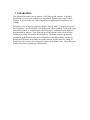
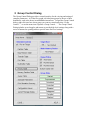
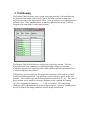
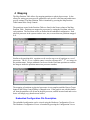
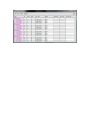
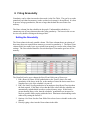
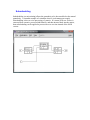
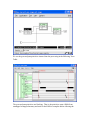
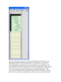
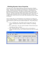
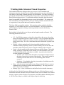
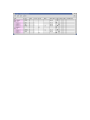
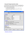
Gedae Compiler User’s Manual
June 22, 2010
Address:
Gedae, Inc.
1247 N Church St, STE 5
Moorestown, NJ 08057
Telephone: (856) 231-4458
FAX:
(856) 231-1403
Internet:
www.gedae.com
Table of Contents
1
2
3
4
Introduction ................................................................................................................. 4
Group Control Dialog ................................................................................................. 5
Partitioning.................................................................................................................. 6
Mapping ...................................................................................................................... 8
Embedded Configuration File Description ..................................................................... 8
Setting Trace Buffer Size and Memory Type ................................................................. 9
Setting Processor Parameters .......................................................................................... 9
Setting the Target Host ................................................................................................. 10
5 Transfer Method Control .......................................................................................... 11
Setting the Transfer Method ......................................................................................... 11
Setting Transfer Method Parameters ............................................................................ 11
6 Firing Granularity ..................................................................................................... 13
Setting the Granularity .................................................................................................. 13
Subscheduling ............................................................................................................... 14
7 Multibuffering Unmapped Memory Transfers ......................................................... 15
8 Priority Table ............................................................................................................ 22
9 Memory Packing Control .......................................................................................... 23
10 Setting Dynamic Queue Properties ........................................................................... 24
11 Setting Static Schedule Thread Properties ................................................................ 25
12 Launch Package Generation Control ........................................................................ 27
Parameters and Queues ................................................................................................. 27
Executables ................................................................................................................... 28
Launch Package ............................................................................................................ 28
1 Introduction
This document describes various features of the Gedae graph compiler. It includes
descriptions of various user controls over compilation, primarily the Group Control
Dialogs. It also describes how Gedae implements an application in response to user
settings.
The primary way of entering compiler settings is through tables. The tables have a few
basic properties. Any field with a white background can be modified. Fields with a grey
background cannot. A field that ends with an asterisk (*) indicates that the field has
been modified by the user. Text displayed in red indicates the value is derived from
another user setting. Most tables are hierarchical. The name column is grouped by
schedule or graph hierarchy that can be collapsed or expanded by double clicking or
through the Edit menu. Most tables have menu items in the Edit menu for setting all
items to the same value or for resetting all values to their default value. Most tables have
a Help menu item to explain basic functionality.
2 Group Control Dialog
The Group Control Dialog provides a central interface for the viewing and setting of
compiler parameters. A Gedae flow graph is divided into groups by the use of host
boundaries, such as the boxes in embeddable/stream/host. To open the Group Control
dialog, right click on a box whose group you want to control and select “Group
Control…” or use the menu item “Options->Group Control…” The Group Control
Dialog includes several toggles and menus to provide high level settings along with a
series of buttons for opening tables to provide more fine level settings.
3 Partitioning
The Partition Table allows the user to group boxes into partitions. It is launched using
the Partition Table button on the Group Control. Partitions can then be mapped to
physical processors in the Map Partition Table. Users group boxes by assigning boxes to
partition names. These partition names are arbitrary alphanumeric strings. Each box
assigned to the same name is in the same partition.
The Partition Table lists all the boxes in the group in the Name column. The list is
hierarchical and can be expanded or collapsed by double clicking on each name.
Assigning a parent box to a partition causes all the children and other descendent boxes
to also be assigned to that partition.
If families are used in creating the flow graph, then equations can be used to set family
members to different partitions. The equations consist of integers, quoted strings and
variables. The variables represent the family dimension and are $1, $2, etc. The value of
these variables can be modified via integer arithmetic in the equation, for example,
($1+100), supporting the operators +, -, *, /, and % (modulus). The result of this
arithmetic can be concatenated with quoted strings using the + operator. Parentheses can
be used to separate the integer arithmetic from the string concatenation.
4 Mapping
The Map Partition Table allows for mapping partitions to physical processors. It also
allows for setting processor-specific parameters such as trace collection and architecturespecific settings. The Map Partition Table is launched by pressing the Map Partition
Table button in the Group Control.
The partitions created in the Partition Table are listed in the Name column of the Map
Partition Table. Partitions are mapped to processors by setting the ProcNum values for
each partition. The ProcNum values are defined in the embedded configuration. Each
physical processor in the system can have zero, one, or more than one partitions mapped
to it.
Similar to the partition table, equations can be used to map a set of partitions to a set of
processors. The $1, $2, etc. variable syntax is used to reference the 1st, 2nd, etc. integer in
the partition name. Integer arithmetic can be used in the ProcNum equations to translate
the integers inside the partition names into processor numbers.
The mapping of partitions to physical processors is not complete until the Run on Target
button in the Group Control Dialog is changed to on. If the graph is run with this button
off, then the partitions will all run on the host processor, and the inserted send and receive
boxes will simply copy data between buffers.
Embedded Configuration File Description
The embedded configuration can be viewed using the Hardware Configuration Viewer.
The Hardware Configuration Viewer is launched by pressing the Configuration Viewer
button in the Group Control. The viewer lists each physical processor in the system. It
has four columns




Name: the integer processor number.
Physical Proc: the hostname (or I.P. address) of the processor where “local”
indicates the same processor as the development environment.
System: the name of the board support package partitions mapped to this
processor will use.
Type: the processor type.
Setting Trace Buffer Size and Memory Type
The Map Partition Table can also be used to customize trace collection. Trace events are
shown in the Trace Table. The Map Partition Table is used to control how much space is
available for trace events and what memory partition those events are stored in. Trace
collection uses a circular buffer; the size of the buffer correlates to the duration of time
shown in the table. The Trace Size column is used to specify the size of the buffer. The
values are entered in number of bytes. Equations can be used to set the size for all
partitions. The Trace MemType column is used to store the events in a specific memory
bank or buffer. For example, on the Cell/B.E. processor, the user may wish to store
events in system memory instead of in SPE local storage to save local storage for more
vital program data.
Setting Processor Parameters
Each board support package has several processor-specific parameters available. These
parameters can be entered into the Params column of the Map Partition Table. To find
out what parameters are available for the current hardware, select Options->View
Settable Params…
Setting the Target Host
The Target Host area of the Group Control can be used to specify a host for the
application other than the development host. This target host can be any processor in the
embedded configuration, simply press the “Set” button in the group control and enter the
processor ID number of the selected physical processor. When it is selected, the
processor numbers in the Mapping Table now reference the embedded configuration file
named after the target host. For example, if the development host is a Linux x86
workstation and processor 100 is a Power Processing Element (PPE) of a Cell Broadband
Engine processor on the same network as the x86, one should set the target host to 100 to
gain access to the SPEs (Synergistic Processing Elements) underneath the PPE. Consult
the Embedded Configuration Manual for more information on setting up hierarchical
embedded configuration files.
The CP column of the Map Partition Table is used to specify which processor runs the
command program. Selecting this option forces the group’s target host to be set to the
development host. Command programs generated while using the CP column setting
require that each generated executable be explicitly started without help from the
command program.
5 Transfer Method Control
The Transfer Table is used to set communication properties for any processor to
processor connection and is launched by pressing the Transfer Table button in the Group
Control. If two kernels are connected by an arc and mapped to different processors, then
a transfer is automatically inserted between the two kernels to send the data. Each of
these transfers is listed in the table. A board support package may provide multiple
transfer methods for the target hardware, and each transfer method may have parameters
that can be set to optimize the transfer’s performance.
The table lists the transfers according to the name of the destination of the transfer, that
is, the input to the kernel that receives the data. The table also lists an Id number for the
transfer. This Id number is used in the name of the send and receive kernels inserted into
the application (for example, “send_13”), and the names are useful for tracking transfers
in the Trace Table and other debugging dialogs. The table also lists the source and
destination processor id number.
Setting the Transfer Method
The transfer method is selected in the Xfer Type column. There are two main types of
transfers – streaming transfers and DMA transfers (direct memory access).
Setting Transfer Method Parameters
Streaming transfers, such as sockets, have an NBsize parameter. The NBsize specifies
the size of the buffer and, if set high enough, can ensure the transfer is nonblocking. The
column can be set to an integer number of bytes or to the string “nb” to allow Gedae to
determine the size of the buffer required to make the transfer nonblocking.
DMA transfers allow both the sends and receives to be multibuffered. The Send Bufs
and Recv Bufs columns allow the user to specify the number of buffers to use in the
multibuffering scheme for each transfer.
Additional parameters may be available for the target system and can be set in the Xfer
Params column.
6 Firing Granularity
Granularity can be either increased or decreased via the Fire Table. The goal is to set the
granularity such that fast memory (cache or other local storage) is best utilized. It is best
to process at large granularities, but not so large that the data does not fit into fast
memory.
The Name column lists the schedules in the graph. Underneath the schedules, it
enumerates sets of boxes that must have the same granularity. The boxes in the set can
be viewed by double clicking on the integer label.
Setting the Granularity
The Gran column is the only settable column. The Bytes column shows an estimate of
how many bytes are required from memory to execute at granularity 1. The Bytes*Gran
column shows how many bytes are required from memory to execute at the current Gran
settings. The Gran column should be set such that Bytes*Gran makes good use of fast
memory.
The Gran field can be set to change the Byes*Gran field in one of four ways:
1. Edit->Reset All Grans: Set all granularities to the Total G (that is, the total
granularity of the boxes in the set, or the number of times the boxes must fire to
complete one cycle of the schedule it is part of).
2. Edit->Set Limit: Set all granularities in an attempt to keep Bytes*Gran less than
the limit entered. If this limit is less than the Bytes value, then the schedules are
automatically subscheduled in order to reduce memory usage. If this limit is
greater than the Bytes value, then the schedules’ granularities are increased as
much as possible while staying within the limit. Maximum subscheduling can be
achieved by setting the limit to 0.
3. Options->Set Gran: Sets the Gran field of the selected set or schedule to the value
entered.
4. Directly typing values into the Gran column in the table.
Subscheduling
Subscheduling (or strip-mining) allows the granularity to be decreased below the natural
granularity. A common example of a situation where it is advantageous to apply
subscheduling is the row-wise processing of a matrix. If a stream of R row vectors is
extracted from a matrix, processed individually, and then inserted back into the matrix,
then subscheduling can be applied to process one row at a time instead of the full R
vectors.
7 Multibuffering Unmapped Memory Transfers
Mapped memory is normal processor memory that can be accessed by dereferencing
pointers to the memory. Unmapped memory is memory that can only be accessed via a
set of functions that move data between unmapped and mapped memory. Some BSPs
provide the ability to allocate large memory blocks that are unmapped. For example, the
Gedae SPU BSP that runs on Cell/B.E SPU processors allows memory areas to be
declared unmapped. The Gedae functions supporting the transfer of data between
unmapped and mapped memory are defined in the Gedae Primitive Function Reference
Manual. These functions include both blocking and nonblocking versions of functions
for moving data between mapped and unmapped memory. Variants of these functions
are also available for moving data between subtiles in unmapped memory into a
contiguous matrix in mapped memory.
Gedae allows users to declare that primitive inputs or outputs are in unmapped memory
(see the Gedae Primitive Programmers Manual). Zero-copy data-reorg primitives are
primitives whose inputs are inplace with their outputs and do not modify the values of the
data, but merely reinterpret it. If the input or output of a zero-copy primitive is
connected to an unmapped memory, then the other input or output and its inplace
counterpart are both declared unmapped. Thus starting at a primitive whose port is
declared unmapped, Gedae propagates this unmapped status through all zero-copy
primitives. When a port that is marked unmapped is connected to a non-zero copy
primitive whose port is not unmapped, then Gedae automatically inserts a primitive to
move data between the unmapped and mapped ports.
For example, consider the following graph. In this graph the mzt_vzt box is a zero-copy
box that is connected at a higher level to unmapped memory so its memory ports are
unmapped. It is connected to the vz_range processing graph that consists of a vz_multV
followed by a vz_fft. These primitives modify the data and their ports are therefore
mapped. Following the vz_range is a vzt_mzt box whose ports are again unmapped.
When Gedae schedules the execution of these primitives it must insert getu primitives
between the mzt_vzt box and the vz_multV box. (It must insert two primitives since the
split complex data is really two data streams.) Following the vz_fft Gedae schedules two
putu primitives to move the data between the mapped vz_fft memory and the unmapped
vzt_mzt input pointer.
We see the getu and putu primitives inserted into the processing in the following Trace
Table:
The getu and putu primitives are blocking. That is, the primitives start a DMA from
unmapped to mapped memory and wait for the DMA to complete before allowing the
processing of the data to continue. Gedae allows the user to specify using a double
buffering scheme to avoid waiting for the DMA’s to complete until after one cycle of the
schedule has executed. Double buffering allows processing to be done in parallel with IO
and improves performance.
A user can enable double buffering using the Group Control Dialog Multi-Buffer Table.
Gedae detects which subschedules can benefit from multibuffering and lists them by
subschedule number in the Multibuffering tool. The user can expand any subschedule to
see what primitives are contained in that subschedule. The user can turn on
Multibuffering on individual subschedules by toggling the MB field. The user can turn
on Multibuffering on all subschedules by selecting Edit->Set All MB Entries and setting
the entries to the value “1”.
When Multibuffering is enabled the subschedule is split into as many as three different
subschedules that have the suffixes get, exec and put. The get subschedule is responsible
for kicking off the DMAs to fetch data from unmapped memory, the exec subschedule is
responsible for processing data and the put subschedule is responsible for kicking of
DMAs to write data back to unmapped memory. Wait primitives are scheduled at
appropriate places to wait for DMAs to complete but only after a full cycle of the
schedule processing is done.
The Trace Table below shows the execution of a multibuffered subschedule. At the
beginning of subscheduling, the get subschedule is executed twice. Two buffers are
fetched during this time. The first buffer will be used by the first firing of the exec
subschedule and the second buffer by the second firing of the exec subschedule. The
exec subschedule will wait for a get buffer, but once in the steady state it will do this only
after a full cycle of exec processing is complete. Thus, the input DMA is overlapped
with one cycle of the processing. Similarly there are multiple output buffers. The
put_nw kicks off a DMA from an output buffer but only waits for the DMA to complete
after one full cycle of the processing when it will be necessary to use the buffer again.
The arrows in the diagram below show which the wait kernels that are associated with the
get_nw and put_nw primitive executions.
Below we see that when the subscheduling of the input matrix completes on the last cycle
a get is not executed because the buffer to be processed was already retrieved on the
previous cycle. However, a wait is invisibly executed at 1 to implement the wait that is a
part of the get schedule. After the last cycle, two wait kernels that were invisibly issued
at 2 by the Gedae wait for the last two put schedule executions that do not have
corresponding waits.
1
2
While the above Trace Tables illustrate how the multibuffering works, they do not show
a great benefit in efficiency because in these examples the vz_vmultV and vz_fft are long
compared to the getu and putu. The processing is CPU bound. When the processing
times are shorter – as they are when running on the Cell/B.E.-- the processing becomes
I/O bound, and the multibuffering becomes important and can greatly reduce the
processing time.
Gedae automatically insert different primitives to move data between unmapped and
mapped memory depending on whether the buffers are tiled or not and depending on if
multibuffering is turned on or not. In addition, even if the memory on both sides of a
connection is mapped but one side is tiled and the tile is embedded in a larger matrix and
the other side of the connection is not tiled, then Gedae automatically inserts a box to
move data from the tile to the non-tiled port. A summary of the different types of
primitives that can be added in all of these cases is illustrated in the table below. If the
Get/Put column is labeled get, then the Unmapped and Tiled columns apply to the source
port of the connection requiring a translation primitive. If the column is labeled put, then
the Unmapped and Tiled columns apply to the destination port of the connection.
Get/Put Unmapped Tiled Multibuffer Box Name
get
no
no
x
no function needed
internal/mt_m
get
no
yes
x
get
get
get
get
put
put
put
put
put
put
yes
yes
yes
yes
no
no
yes
yes
yes
yes
no
no
yes
yes
no
yes
no
no
yes
yes
no
yes
no
yes
x
x
no
yes
no
yes
internal/getu
internal/getu_nw
internal/mtu_m
internal/mtu_m_nw
no function needed
internal/m_mt
internal/putu
internal/putu_nw
internal/m_mtu
internal/m_mtu_nw
Note, a transfer port is not considered tile if the tile size only differs in the row
dimension. That is, a matrix out[256:512][128:128] connected to a matrix
in[256][128] does required a tiled transfer. In this case a getu or getu_nw
transfer primitive is inserted if the out source is unmapped.
8 Priority Table
A schedule orders the execution of kernels. Scheduling, that is, the creation of schedules,
happens during compilation. Several orderings may be possible. The user may wish to
order the kernels in a specific way to handle external side effects, order sends and
receives, etc. This ordering can be affected by the user through the setting of priorities.
Because Gedae cannot create an illegal schedule, some priority settings may have no
effect.
The default priority for each kernel is 0. Setting a priority to a positive number moves it
up in the schedule, that is, it will potentially fire earlier. Setting a priority to a negative
number moves it down in the schedule.
9 Memory Packing Control
The Static Memory Packer Pulldown Menu in the Group Control Dialog allows selecting
between different memory packing algorithms. All memory packing is done during
compilation, but larger applications may wish to use more lightweight algorithms to
reduce compile time at the price of memory usage. The default is Fast Packer – a
lightweight algorithm. Single Block Packer and Multi Block Packer provide
progressively better packing but take longer to calculate the packing. No Packing is
available to skip memory packing altogether.
10 Setting Dynamic Queue Properties
The Queue Table is used to display information and control the capacity of dynamic
queues. The Queue Table is launched by pressing the Queue Table button in the Group
Control. The table lists all the dynamic queues in the group. The Name shows the
destination of the dynamic queue. The Capacity is shown in number of tokens, where
Bytes is the storage size allocated to hold this capacity, that is, the capacity times the
token size. The Memory Type shows which memory bank the queue is allocated in, and
if multiple banks are available, allows for the mapping of the queue to memory. For
example on the Cell/B.E. processor, the user may wish to map queues to huge TLB pages
for efficiency.
The Src and Dest Policy provide information on when schedules fire according to the
presence of tokens in the queue. The Src Policy specifies when the source schedule fires,
and the Dest Policy specifies when the destination schedule fires. The possible policies
are:
 cont – a controlling queue. The schedule will fire if any tokens or space are
available, shrinking itself to handle the smallest availability on a controlling
queue.
 req – a required queue. The queue requires the number of tokens dictated by the
controlling queues before it will fire.
 n-req – a non-required queue. The schedule can fire even if no tokens are
available on the queue and may, while running, determine that tokens are actually
needed.
11 Setting Static Schedule Thread Properties
The Schedule Parameters dialog provides easy access to a list of schedules and
information about the schedules, such as finding what primitives are in each schedule. It
also allows for the setting of thread properties for the schedules. The table is opened by
pressing the Schedule Parameters dialog in the Group Control. Each schedule acts like a
thread on the target processors. If a partition has multiple schedules, then the runtime
kernel is responsible for determining when to execute each schedule. The settings and
data in this dialog can help describe the policy for running schedules and allow the user
to set priorities, to set periods and to retry times for schedules.
The Name field is grouped by partition. Each partition can have multiple schedules
mapped to it. Each schedule may have several subschedules. The Name column may
also list Memory Segments, relating to memory partitions created in the Memory
Partition Table.
Each schedule is listed with its size in bytes and its length in number of kernels. The
following parameters can be set:





OV – For BSPs that support overlays this column allows the user to select what
parts of the application go into a separate overlay. If set for a partition then Reset
methods are place in their own overlay. If set for a schedule then the schedule is
placed in an overlay. If set for a subschedule then the subschedule is placed in an
overlay.
Priority – aids the runtime kernel in choosing which schedule to run first.
Schedules with larger priority (closest to positive infinity) will execute first, and
schedules with lowest priority (closest to negative infinity) will execute last.
Period – tells the runtime kernel the period between schedule firings. The default
setting, relating to a blank entry in the column, is to follow dataflow policy, that
is, the schedule should fire when data is available. A period can be entered in
seconds or number of schedules.
o Seconds – if in seconds, then the number of seconds must elapse between
the start of successive execution of the schedule. This period is useful for
emulating real-time data sources or for monitoring other external
resources.
o Schedules – if in schedules, then the given number of schedules must fire
before this schedule fires again.
Retry – tells the runtime kernel when to retry firing a schedule if there is an error
condition such as a primitive calling embSuspendRetry(). The retry period can
also be in seconds or schedules.
Memory Type – where to allocate the data buffers for the schedule in memory.
Additionally, the Schedule Parameters dialog provides a set of Boolean flags to specify
information about the schedule used by the runtime kernel, such as whether it uses shared
memory, requires exclusive locks to access memory, and other runtime scheduling issues.
A full list of these flags is available in the Help message for the dialog.
12 Launch Package Generation Control
A Launch Package is a directory containing executables that allow a single group to be
executed independently from the development environment. A command program is also
generated to control the loading, launching and execution of all the executables. There
are three options for using this launch package:
 As a standalone, deliverable application
 As a parent application integrating with non-Gedae components through
customization of the command program
 As a child function through use of the function interface to the command
program.
Parameters and Queues
The Parameters and Queues visible to external software are listed in the dialog. The
default names of these data are based on the hierarchy of the flow graph. Shorter names
can be given by specifying Synonyms. The Parameters are all parameters that can be
changed at runtime; the compiler aggressively precomputes parameters to avoid runtime
recalculation. The Queues are the boundaries between groups created by the boxes in the
embeddable/stream/host directory.
Executables
The executable creation can also be customized to best suit the target hardware. Note:
target hardware provides a target-specific value of these settings. The settings are
 Create Schedules in Command Program – The schedule information is contained
in the command program and sent to the target processors at start up.
o Create Target Executables As Arrays in Command Program – This option
code generates binary arrays representing target executables into the
command program. The option may not be available on all target
processors.
o Create Unified Target Executable – This option creates one executable
containing all partitions and all kernels of the graph. This option reduces
the storage requirements as only one executable is created and can be used
to support targets that require SPMD (Single Program Multiple Data).
 Create Schedules in Target Executables (No Host) – Target executables are
completely self-contained and start up without host intervention. Note: running
without host intervention disables useful debugging features such as trace
collection.
Launch Package
The command program can be customized using the Command Program Interface. The
directory to store the launch package, any customizations to the command program C
source file, and libraries or object files to link with the command program can be placed
in the Command Program section of the dialog. Each of these entries is a path to the
corresponding directory or file(s).