Download QGIS User Guide - OSGeo Server

Quantum GIS
User Guide
Version 1.4.0 ’Enceladus’
Preamble
This document is the original user guide of the described software Quantum GIS. The software and
hardware described in this document are in most cases registered trademarks and are therefore
subject to the legal requirements. Quantum GIS is subject to the GNU General Public License. Find
more information on the Quantum GIS Homepage http://qgis.osgeo.org.
The details, data, results etc. in this document have been written and verified to the best of knowledge
and responsibility of the authors and editors. Nevertheless, mistakes concerning the content are
possible.
Therefore, all data are not liable to any duties or guarantees. The authors, editors and publishers do
not take any responsibility or liability for failures and their consequences. Your are always welcome
to indicate possible mistakes.
This document has been typeset with LATEX. It is available as LATEX source code via subversion and
online as PDF document via http://qgis.osgeo.org/documentation/manuals.html. Translated
versions of this document can be downloaded via the documentation area of the QGIS project as
well. For more information about contributing to this document and about translating it, please visit:
http://www.qgis.org/wiki/
Links in this Document
This document contains internal and external links. Clicking on an internal link moves within the
document, while clicking on an external link opens an internet address. In PDF form, internal links
are shown in blue, while external links are shown in red and are handled by the system browser. In
HTML form, the browser displays and handles both identically.
User, Installation and Coding Guide Authors and Editors:
Tara Athan
Otto Dassau
Anne Ghisla
Magnus Homann
Werner Macho
Gary E. Sherman
Radim Blazek
Martin Dobias
Stephan Holl
K. Koy
Carson J.Q. Farmer
Tim Sutton
Godofredo Contreras
Peter Ersts
N. Horning
Lars Luthman
Tyler Mitchell
David Willis
Claudia A. Engel
Jürgen E. Fischer
Marco Hugentobler
Gavin Macaulay
Brendan Morely
With thanks to Tisham Dhar for preparing the initial msys (MS Windows) environment
documentation, to Tom Elwertowski and William Kyngesburye for help in the MAC OSX Installation
Section and to Carlos Dávila, Paolo Cavallini and Christian Gunning for revisions. If we have
neglected to mention any contributors, please accept our apologies for this oversight.
c 2004 - 2010 Quantum GIS Development Team
Copyright °
Internet: http://qgis.osgeo.org
License of this document
Permission is granted to copy, distribute and/or modify this document under the terms of the GNU
Free Documentation License, Version 1.3 or any later version published by the Free Software Foundation; with no Invariant Sections, no Front-Cover Texts and no Back-Cover Texts. A copy of the
license is included in section D entitled "GNU Free Documentation License".
QGIS 1.4.0 User Guide
iii
Contents
Contents
Title
i
Preamble
ii
Table of Contents
iv
List of Figures
x
List of Tables
xiii
List of QGIS Tips
xv
1. Foreword
1.1. Features . . . . . . . . . . . . . . . . . . . . . . . . . . . . . . . . . . . . . . . . . . . .
1.1.1. What’s new in version 1.4.0 . . . . . . . . . . . . . . . . . . . . . . . . . . . . .
1.2. Conventions . . . . . . . . . . . . . . . . . . . . . . . . . . . . . . . . . . . . . . . . . .
1
1
4
6
2. Introduction To GIS
2.1. Why is all this so new? . . . . . . . . . . . . . . . . . . . . . . . . . . . . . . . . . . . .
2.1.1. Raster Data . . . . . . . . . . . . . . . . . . . . . . . . . . . . . . . . . . . . . .
2.1.2. Vector Data . . . . . . . . . . . . . . . . . . . . . . . . . . . . . . . . . . . . . .
9
10
10
11
3. Getting Started
3.1. Installation . . . . . . . . . . . . . . . . . . . . . . . . . . . . . . . . . . . . . . . . . .
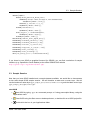
3.2. Sample Data . . . . . . . . . . . . . . . . . . . . . . . . . . . . . . . . . . . . . . . . .
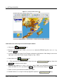
3.3. Sample Session . . . . . . . . . . . . . . . . . . . . . . . . . . . . . . . . . . . . . . .
12
12
12
13
4. Features at a Glance
4.1. Starting and Stopping QGIS . . . . .
4.1.1. Command Line Options . . .
4.2. QGIS GUI . . . . . . . . . . . . . . .
4.2.1. Keyboard shortcuts . . . . .
4.2.2. Menu Bar . . . . . . . . . . .
4.2.3. Toolbars . . . . . . . . . . . .
4.2.4. Map Legend . . . . . . . . .
4.2.5. Map View . . . . . . . . . . .
4.2.6. Map Overview . . . . . . . .
4.2.7. Status Bar . . . . . . . . . . .
4.3. Rendering . . . . . . . . . . . . . . .
4.3.1. Scale Dependent Rendering
4.3.2. Controlling Map Rendering .
4.4. Measuring . . . . . . . . . . . . . . .
16
16
16
18
19
19
23
23
25
26
26
26
27
27
28
QGIS 1.4.0 User Guide
.
.
.
.
.
.
.
.
.
.
.
.
.
.
.
.
.
.
.
.
.
.
.
.
.
.
.
.
.
.
.
.
.
.
.
.
.
.
.
.
.
.
.
.
.
.
.
.
.
.
.
.
.
.
.
.
.
.
.
.
.
.
.
.
.
.
.
.
.
.
.
.
.
.
.
.
.
.
.
.
.
.
.
.
.
.
.
.
.
.
.
.
.
.
.
.
.
.
.
.
.
.
.
.
.
.
.
.
.
.
.
.
.
.
.
.
.
.
.
.
.
.
.
.
.
.
.
.
.
.
.
.
.
.
.
.
.
.
.
.
.
.
.
.
.
.
.
.
.
.
.
.
.
.
.
.
.
.
.
.
.
.
.
.
.
.
.
.
.
.
.
.
.
.
.
.
.
.
.
.
.
.
.
.
.
.
.
.
.
.
.
.
.
.
.
.
.
.
.
.
.
.
.
.
.
.
.
.
.
.
.
.
.
.
.
.
.
.
.
.
.
.
.
.
.
.
.
.
.
.
.
.
.
.
.
.
.
.
.
.
.
.
.
.
.
.
.
.
.
.
.
.
.
.
.
.
.
.
.
.
.
.
.
.
.
.
.
.
.
.
.
.
.
.
.
.
.
.
.
.
.
.
.
.
.
.
.
.
.
.
.
.
.
.
.
.
.
.
.
.
.
.
.
.
.
.
.
.
.
.
.
.
.
.
.
.
.
.
.
.
.
.
.
.
.
.
.
.
.
.
.
.
.
.
.
.
.
.
.
.
.
.
.
.
.
.
.
.
.
.
.
.
.
.
.
.
.
.
.
.
.
.
.
.
.
.
.
.
.
.
.
.
.
.
.
.
.
.
.
.
.
.
.
.
.
.
.
.
.
.
.
.
iv
Contents
4.5.
4.6.
4.7.
4.8.
4.4.1. Measure length and areas
Projects . . . . . . . . . . . . . .
Output . . . . . . . . . . . . . . .
GUI Options . . . . . . . . . . . .
Spatial Bookmarks . . . . . . . .
4.8.1. Creating a Bookmark . .
4.8.2. Working with Bookmarks
4.8.3. Zooming to a Bookmark .
4.8.4. Deleting a Bookmark . . .
.
.
.
.
.
.
.
.
.
.
.
.
.
.
.
.
.
.
.
.
.
.
.
.
.
.
.
.
.
.
.
.
.
.
.
.
.
.
.
.
.
.
.
.
.
.
.
.
.
.
.
.
.
.
.
.
.
.
.
.
.
.
.
.
.
.
.
.
.
.
.
.
.
.
.
.
.
.
.
.
.
.
.
.
.
.
.
.
.
.
.
.
.
.
.
.
.
.
.
.
.
.
.
.
.
.
.
.
.
.
.
.
.
.
.
.
.
.
.
.
.
.
.
.
.
.
.
.
.
.
.
.
.
.
.
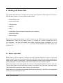
5. Working with Vector Data
5.1. ESRI Shapefiles . . . . . . . . . . . . . . . . . . . . . . . .
5.1.1. Loading a Shapefile . . . . . . . . . . . . . . . . . .
5.1.2. Improving Performance . . . . . . . . . . . . . . . .
5.1.3. Loading a MapInfo Layer . . . . . . . . . . . . . . .
5.1.4. Loading an ArcInfo Binary Coverage . . . . . . . . .
5.2. PostGIS Layers . . . . . . . . . . . . . . . . . . . . . . . . .
5.2.1. Creating a stored Connection . . . . . . . . . . . . .
5.2.2. Loading a PostGIS Layer . . . . . . . . . . . . . . .
5.2.3. Some details about PostgreSQL layers . . . . . . .
5.2.4. Importing Data into PostgreSQL . . . . . . . . . . .
5.2.5. Improving Performance . . . . . . . . . . . . . . . .
5.2.6. Vector layers crossing 180◦ longitude . . . . . . . .
5.3. SpatiaLite Layers . . . . . . . . . . . . . . . . . . . . . . . .
5.4. The Vector Properties Dialog . . . . . . . . . . . . . . . . .
5.4.1. Symbology Tab . . . . . . . . . . . . . . . . . . . . .
5.4.2. New Generation Symbology . . . . . . . . . . . . . .
5.4.3. Working with the New Generation Symbology . . . .
5.4.4. Style Manager to manage symbols and color ramps
5.4.5. Labels Tab . . . . . . . . . . . . . . . . . . . . . . .
5.4.6. Attributes Tab . . . . . . . . . . . . . . . . . . . . . .
5.4.7. General Tab . . . . . . . . . . . . . . . . . . . . . . .
5.4.8. Metadata Tab . . . . . . . . . . . . . . . . . . . . . .
5.4.9. Actions Tab . . . . . . . . . . . . . . . . . . . . . . .
5.4.10. Diagram Tab . . . . . . . . . . . . . . . . . . . . . .
5.5. Editing . . . . . . . . . . . . . . . . . . . . . . . . . . . . . .
5.5.1. Setting the Snapping Tolerance and Search Radius
5.5.2. Zooming and Panning . . . . . . . . . . . . . . . . .
5.5.3. Topological editing . . . . . . . . . . . . . . . . . . .
5.5.4. Digitizing an existing layer . . . . . . . . . . . . . . .
5.5.5. Advanced digitizing . . . . . . . . . . . . . . . . . .
5.5.6. Creating a New Layer . . . . . . . . . . . . . . . . .
QGIS 1.4.0 User Guide
.
.
.
.
.
.
.
.
.
.
.
.
.
.
.
.
.
.
.
.
.
.
.
.
.
.
.
.
.
.
.
.
.
.
.
.
.
.
.
.
.
.
.
.
.
.
.
.
.
.
.
.
.
.
.
.
.
.
.
.
.
.
.
.
.
.
.
.
.
.
.
.
.
.
.
.
.
.
.
.
.
.
.
.
.
.
.
.
.
.
.
.
.
.
.
.
.
.
.
.
.
.
.
.
.
.
.
.
.
.
.
.
.
.
.
.
.
.
.
.
.
.
.
.
.
.
.
.
.
.
.
.
.
.
.
.
.
.
.
.
.
.
.
.
.
.
.
.
.
.
.
.
.
.
.
.
.
.
.
.
.
.
.
.
.
.
.
.
.
.
.
.
.
.
.
.
.
.
.
.
.
.
.
.
.
.
.
.
.
.
.
.
.
.
.
.
.
.
.
.
.
.
.
.
.
.
.
.
.
.
.
.
.
.
.
.
.
.
.
.
.
.
.
.
.
.
.
.
.
.
.
.
.
.
.
.
.
.
.
.
.
.
.
.
.
.
.
.
.
.
.
.
.
.
.
.
.
.
.
.
.
.
.
.
.
.
.
.
.
.
.
.
.
.
.
.
.
.
.
.
.
.
.
.
.
.
.
.
.
.
.
.
.
.
.
.
.
.
.
.
.
.
.
.
.
.
.
.
.
.
.
.
.
.
.
.
.
.
.
.
.
.
.
.
.
.
.
.
.
.
.
.
.
.
.
.
.
.
.
.
.
.
.
.
.
.
.
.
.
.
.
.
.
.
.
.
.
.
.
.
.
.
.
.
.
.
.
.
.
.
.
.
.
.
.
.
.
.
.
.
.
.
.
.
.
.
.
.
.
.
.
.
.
.
.
.
.
.
.
.
.
.
.
.
.
.
.
.
.
.
.
.
.
.
.
.
.
.
.
.
.
.
.
.
.
.
.
.
.
.
.
.
.
.
.
.
.
.
.
.
.
.
.
.
.
.
.
.
.
.
.
.
.
.
.
.
.
.
.
.
.
.
.
.
.
.
.
.
.
.
.
.
.
.
.
.
.
.
.
.
.
.
.
.
.
.
.
.
.
.
.
.
.
.
.
.
.
.
.
.
.
.
.
.
.
.
.
.
.
.
.
.
.
.
.
.
.
.
.
.
.
.
.
.
.
.
.
.
.
.
.
.
.
.
.
.
.
.
.
.
.
.
.
.
.
.
.
.
.
.
.
.
.
.
.
.
.
.
.
.
.
.
.
.
.
.
.
.
.
29
29
30
31
35
35
35
35
35
.
.
.
.
.
.
.
.
.
.
.
.
.
.
.
.
.
.
.
.
.
.
.
.
.
.
.
.
.
.
.
36
36
37
38
39
40
40
40
42
42
43
44
45
46
47
48
49
51
54
55
56
58
58
58
62
63
63
66
66
67
72
75
v
Contents
5.5.7. Working with the Attribute Table . . . . . . . . . . . . . . . . . . . . . . . . . .
5.6. Query Builder . . . . . . . . . . . . . . . . . . . . . . . . . . . . . . . . . . . . . . . . .
5.7. Field Calculator . . . . . . . . . . . . . . . . . . . . . . . . . . . . . . . . . . . . . . . .
6. Working with Raster Data
6.1. What is raster data? . . . .
6.2. Loading raster data in QGIS
6.3. Raster Properties Dialog . .
6.3.1. Symbology Tab . . .
6.3.2. Transparency Tab .
6.3.3. Colormap . . . . . .
6.3.4. General Tab . . . . .
6.3.5. Metadata Tab . . . .
6.3.6. Pyramids Tab . . . .
6.3.7. Histogram Tab . . .
76
78
80
.
.
.
.
.
.
.
.
.
.
.
.
.
.
.
.
.
.
.
.
.
.
.
.
.
.
.
.
.
.
.
.
.
.
.
.
.
.
.
.
.
.
.
.
.
.
.
.
.
.
.
.
.
.
.
.
.
.
.
.
.
.
.
.
.
.
.
.
.
.
.
.
.
.
.
.
.
.
.
.
.
.
.
.
.
.
.
.
.
.
.
.
.
.
.
.
.
.
.
.
.
.
.
.
.
.
.
.
.
.
.
.
.
.
.
.
.
.
.
.
.
.
.
.
.
.
.
.
.
.
.
.
.
.
.
.
.
.
.
.
.
.
.
.
.
.
.
.
.
.
.
.
.
.
.
.
.
.
.
.
.
.
.
.
.
.
.
.
.
.
.
.
.
.
.
.
.
.
.
.
.
.
.
.
.
.
.
.
.
.
.
.
.
.
.
.
.
.
.
.
.
.
.
.
.
.
.
.
.
.
.
.
.
.
.
.
.
.
.
.
.
.
.
.
.
.
.
.
.
.
.
.
.
.
.
.
.
.
.
.
.
.
.
.
.
.
.
.
.
.
.
.
.
.
.
.
.
.
.
.
.
.
.
.
.
.
.
.
.
.
.
.
.
.
.
.
.
.
.
.
.
.
.
.
.
.
.
.
.
.
.
.
.
.
.
.
.
.
.
.
83
83
84
84
85
87
87
88
88
89
89
7. Working with OGC Data
7.1. What is OGC Data . . . . . . . . .
7.2. WMS Client . . . . . . . . . . . . .
7.2.1. Overview of WMS Support
7.2.2. Selecting WMS Servers . .
7.2.3. Loading WMS Layers . . .
7.2.4. Server-Search . . . . . . .
7.2.5. Using the Identify Tool . . .
7.2.6. Viewing Properties . . . . .
7.2.7. WMS Client Limitations . .
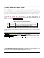
7.3. WFS Client . . . . . . . . . . . . .
7.3.1. Loading a WFS Layer . . .
.
.
.
.
.
.
.
.
.
.
.
.
.
.
.
.
.
.
.
.
.
.
.
.
.
.
.
.
.
.
.
.
.
.
.
.
.
.
.
.
.
.
.
.
.
.
.
.
.
.
.
.
.
.
.
.
.
.
.
.
.
.
.
.
.
.
.
.
.
.
.
.
.
.
.
.
.
.
.
.
.
.
.
.
.
.
.
.
.
.
.
.
.
.
.
.
.
.
.
.
.
.
.
.
.
.
.
.
.
.
.
.
.
.
.
.
.
.
.
.
.
.
.
.
.
.
.
.
.
.
.
.
.
.
.
.
.
.
.
.
.
.
.
.
.
.
.
.
.
.
.
.
.
.
.
.
.
.
.
.
.
.
.
.
.
.
.
.
.
.
.
.
.
.
.
.
.
.
.
.
.
.
.
.
.
.
.
.
.
.
.
.
.
.
.
.
.
.
.
.
.
.
.
.
.
.
.
.
.
.
.
.
.
.
.
.
.
.
.
.
.
.
.
.
.
.
.
.
.
.
.
.
.
.
.
.
.
.
.
.
.
.
.
.
.
.
.
.
.
.
.
.
.
.
.
.
.
.
.
.
.
.
.
.
.
.
.
.
.
.
.
.
.
.
.
.
.
.
.
.
.
.
.
.
.
.
.
.
.
.
.
.
.
.
.
.
.
.
.
.
.
.
.
.
.
.
.
.
.
.
.
.
.
.
.
.
.
.
.
90
90
90
90
91
92
94
95
95
96
97
97
.
.
.
.
.
.
.
.
.
.
.
.
.
.
.
.
.
.
.
.
.
.
.
.
.
.
.
.
.
.
8. Working with Projections
8.1. Overview of Projection Support . . . .
8.2. Specifying a Projection . . . . . . . . .
8.3. Define On The Fly (OTF) Projection .
8.4. Custom Coordinate Reference System
.
.
.
.
.
.
.
.
.
.
.
.
.
.
.
.
.
.
.
.
.
.
.
.
.
.
.
.
.
.
.
.
.
.
.
.
.
.
.
.
.
.
.
.
.
.
.
.
.
.
.
.
.
.
.
.
.
.
.
.
.
.
.
.
.
.
.
.
.
.
.
.
.
.
.
.
.
.
.
.
.
.
.
.
.
.
.
.
.
.
.
.
.
.
.
.
.
.
.
.
100
100
100
101
103
9. GRASS GIS Integration
9.1. Starting the GRASS plugin . . . . . . . . .
9.2. Loading GRASS raster and vector layers . .
9.3. GRASS LOCATION and MAPSET . . . . .
9.3.1. Creating a new GRASS LOCATION
9.3.2. Adding a new MAPSET . . . . . . .
9.4. Importing data into a GRASS LOCATION .
9.5. The GRASS vector data model . . . . . . .
.
.
.
.
.
.
.
.
.
.
.
.
.
.
.
.
.
.
.
.
.
.
.
.
.
.
.
.
.
.
.
.
.
.
.
.
.
.
.
.
.
.
.
.
.
.
.
.
.
.
.
.
.
.
.
.
.
.
.
.
.
.
.
.
.
.
.
.
.
.
.
.
.
.
.
.
.
.
.
.
.
.
.
.
.
.
.
.
.
.
.
.
.
.
.
.
.
.
.
.
.
.
.
.
.
.
.
.
.
.
.
.
.
.
.
.
.
.
.
.
.
.
.
.
.
.
.
.
.
.
.
.
.
.
.
.
.
.
.
.
.
.
.
.
.
.
.
.
.
.
.
.
.
.
.
.
.
.
.
.
.
.
.
.
.
.
.
.
106
106
107
108
109
110
111
112
QGIS 1.4.0 User Guide
.
.
.
.
.
.
.
.
vi
Contents
9.6.
9.7.
9.8.
9.9.
Creating a new GRASS vector layer . . . . . . . . . .
Digitizing and editing a GRASS vector layer . . . . . .
The GRASS region tool . . . . . . . . . . . . . . . . .
The GRASS toolbox . . . . . . . . . . . . . . . . . . .
9.9.1. Working with GRASS modules . . . . . . . . .
9.9.2. GRASS module examples . . . . . . . . . . . .
9.9.3. Working with the GRASS LOCATION browser
9.9.4. Customizing the GRASS Toolbox . . . . . . . .
.
.
.
.
.
.
.
.
.
.
.
.
.
.
.
.
.
.
.
.
.
.
.
.
.
.
.
.
.
.
.
.
.
.
.
.
.
.
.
.
.
.
.
.
.
.
.
.
.
.
.
.
.
.
.
.
.
.
.
.
.
.
.
.
.
.
.
.
.
.
.
.
.
.
.
.
.
.
.
.
.
.
.
.
.
.
.
.
.
.
.
.
.
.
.
.
.
.
.
.
.
.
.
.
.
.
.
.
.
.
.
.
.
.
.
.
.
.
.
.
.
.
.
.
.
.
.
.
.
.
.
.
.
.
.
.
.
.
.
.
.
.
.
.
113
113
117
118
118
120
126
127
10. Print Composer
10.1.Open a new Print Composer Template . . . . . . . . . . . . . . . . . . .
10.2.Using Print Composer . . . . . . . . . . . . . . . . . . . . . . . . . . . .
10.3.Adding a current QGIS map canvas to the Print Composer . . . . . . . .
10.3.1. Map item tab - Map and Extents dialog . . . . . . . . . . . . . .
10.3.2. Map item tab - Grid and General options dialog . . . . . . . . . .
10.4.Adding other elements to the Print Composer . . . . . . . . . . . . . . .
10.4.1. Label item tab - Label and General options dialog . . . . . . . .
10.4.2. Image item tab - Picture options and General options dialog . . .
10.4.3. Legend item tab - General, Legend items and Item option dialog
10.4.4. Scalebar item tab - Scalebar and General options dialog . . . . .
10.5.Navigation tools . . . . . . . . . . . . . . . . . . . . . . . . . . . . . . .
10.6.Add Basic shape and Arrow . . . . . . . . . . . . . . . . . . . . . . . . .
10.7.Raise, lower and align elements . . . . . . . . . . . . . . . . . . . . . .
10.8.Creating Output . . . . . . . . . . . . . . . . . . . . . . . . . . . . . . . .
10.9.Saving and loading a print composer layout . . . . . . . . . . . . . . . .
.
.
.
.
.
.
.
.
.
.
.
.
.
.
.
.
.
.
.
.
.
.
.
.
.
.
.
.
.
.
.
.
.
.
.
.
.
.
.
.
.
.
.
.
.
.
.
.
.
.
.
.
.
.
.
.
.
.
.
.
.
.
.
.
.
.
.
.
.
.
.
.
.
.
.
.
.
.
.
.
.
.
.
.
.
.
.
.
.
.
.
.
.
.
.
.
.
.
.
.
.
.
.
.
.
.
.
.
.
.
.
.
.
.
.
.
.
.
.
.
128
129
129
130
131
132
133
134
135
136
137
138
139
139
140
141
11. QGIS Plugins
11.1.Managing Plugins . . . . . . . . . . . . . . . .
11.1.1. Loading a QGIS Core Plugin . . . . . .
11.1.2. Loading an external QGIS Plugin . . . .
11.1.3. Using the QGIS Python Plugin Installer
11.2.Data Providers . . . . . . . . . . . . . . . . . .
.
.
.
.
.
.
.
.
.
.
.
.
.
.
.
.
.
.
.
.
.
.
.
.
.
.
.
.
.
.
.
.
.
.
.
.
.
.
.
.
142
142
142
143
143
146
.
.
.
.
.
.
.
.
.
147
148
149
149
150
150
152
154
155
155
12. Using QGIS Core Plugins
12.1.Coordinate Capture Plugin .
12.2.Decorations Plugins . . . . .
12.2.1. Copyright Label Plugin
12.2.2. North Arrow Plugin . .
12.2.3. Scale Bar Plugin . . .
12.3.Delimited Text Plugin . . . . .
12.4.Dxf2Shp Converter Plugin . .
12.5.eVis Plugin . . . . . . . . . .
12.5.1. Event Browser . . . .
QGIS 1.4.0 User Guide
.
.
.
.
.
.
.
.
.
.
.
.
.
.
.
.
.
.
.
.
.
.
.
.
.
.
.
.
.
.
.
.
.
.
.
.
.
.
.
.
.
.
.
.
.
.
.
.
.
.
.
.
.
.
.
.
.
.
.
.
.
.
.
.
.
.
.
.
.
.
.
.
.
.
.
.
.
.
.
.
.
.
.
.
.
.
.
.
.
.
.
.
.
.
.
.
.
.
.
.
.
.
.
.
.
.
.
.
.
.
.
.
.
.
.
.
.
.
.
.
.
.
.
.
.
.
.
.
.
.
.
.
.
.
.
.
.
.
.
.
.
.
.
.
.
.
.
.
.
.
.
.
.
.
.
.
.
.
.
.
.
.
.
.
.
.
.
.
.
.
.
.
.
.
.
.
.
.
.
.
.
.
.
.
.
.
.
.
.
.
.
.
.
.
.
.
.
.
.
.
.
.
.
.
.
.
.
.
.
.
.
.
.
.
.
.
.
.
.
.
.
.
.
.
.
.
.
.
.
.
.
.
.
.
.
.
.
.
.
.
.
.
.
.
.
.
.
.
.
.
.
.
.
.
.
.
.
.
.
.
.
.
.
.
.
.
.
.
.
.
.
.
.
.
.
.
.
.
.
.
.
.
.
.
.
.
.
.
.
.
.
.
.
.
.
.
.
.
.
.
.
.
.
.
.
.
.
.
.
.
.
.
.
.
.
.
.
.
.
.
.
.
.
.
.
.
.
.
.
.
.
.
.
.
.
.
.
.
.
.
.
.
.
.
.
.
.
.
.
vii
Contents
12.5.2. Event ID Tool . . . . . . . . . . . . . .
12.5.3. Database connection . . . . . . . . .
12.6.fTools Plugin . . . . . . . . . . . . . . . . . .
12.7.Georeferencer Plugin . . . . . . . . . . . . .
12.8.GPS Plugin . . . . . . . . . . . . . . . . . . .
12.8.1. What is GPS? . . . . . . . . . . . . .
12.8.2. Loading GPS data from a file . . . . .
12.8.3. GPSBabel . . . . . . . . . . . . . . . .
12.8.4. Importing GPS data . . . . . . . . . .
12.8.5. Downloading GPS data from a device
12.8.6. Uploading GPS data to a device . . .
12.8.7. Defining new device types . . . . . . .
12.9.Interpolation Plugin . . . . . . . . . . . . . . .
12.10.Labeling Plugin . . . . . . . . . . . . . . . . .
12.11.MapServer Export Plugin . . . . . . . . . . .
12.11.1.Creating the Project File . . . . . . . .
12.11.2.Creating the Map File . . . . . . . . .
12.11.3.Testing the Map File . . . . . . . . . .
12.12.OGR Converter Plugin . . . . . . . . . . . . .
12.13.Oracle GeoRaster Plugin . . . . . . . . . . .
12.13.1.Managing connections . . . . . . . . .
12.13.2.Selecting a GeoRaster . . . . . . . . .
12.13.3.Displaying GeoRaster . . . . . . . . .
12.14.OpenStreetMap Plugin . . . . . . . . . . . . .
12.14.1.Installation . . . . . . . . . . . . . . .
12.14.2.Basic user interface . . . . . . . . . .
12.14.3.Loading OSM data . . . . . . . . . . .
12.14.4.Viewing OSM data . . . . . . . . . . .
12.14.5.Editing basic OSM data . . . . . . . .
12.14.6.Editing relations . . . . . . . . . . . .
12.14.7.Downloading OSM data . . . . . . . .
12.14.8.Uploading OSM data . . . . . . . . . .
12.14.9.Saving OSM data . . . . . . . . . . .
12.14.10.
Import OSM data . . . . . . . . . . . .
12.15.Raster Terrain Modelling Plugin . . . . . . . .
12.16.Quick Print Plugin . . . . . . . . . . . . . . .
12.17.Other core plugins . . . . . . . . . . . . . . .
13. Using external QGIS Python Plugins
.
.
.
.
.
.
.
.
.
.
.
.
.
.
.
.
.
.
.
.
.
.
.
.
.
.
.
.
.
.
.
.
.
.
.
.
.
.
.
.
.
.
.
.
.
.
.
.
.
.
.
.
.
.
.
.
.
.
.
.
.
.
.
.
.
.
.
.
.
.
.
.
.
.
.
.
.
.
.
.
.
.
.
.
.
.
.
.
.
.
.
.
.
.
.
.
.
.
.
.
.
.
.
.
.
.
.
.
.
.
.
.
.
.
.
.
.
.
.
.
.
.
.
.
.
.
.
.
.
.
.
.
.
.
.
.
.
.
.
.
.
.
.
.
.
.
.
.
.
.
.
.
.
.
.
.
.
.
.
.
.
.
.
.
.
.
.
.
.
.
.
.
.
.
.
.
.
.
.
.
.
.
.
.
.
.
.
.
.
.
.
.
.
.
.
.
.
.
.
.
.
.
.
.
.
.
.
.
.
.
.
.
.
.
.
.
.
.
.
.
.
.
.
.
.
.
.
.
.
.
.
.
.
.
.
.
.
.
.
.
.
.
.
.
.
.
.
.
.
.
.
.
.
.
.
.
.
.
.
.
.
.
.
.
.
.
.
.
.
.
.
.
.
.
.
.
.
.
.
.
.
.
.
.
.
.
.
.
.
.
.
.
.
.
.
.
.
.
.
.
.
.
.
.
.
.
.
.
.
.
.
.
.
.
.
.
.
.
.
.
.
.
.
.
.
.
.
.
.
.
.
.
.
.
.
.
.
.
.
.
.
.
.
.
.
.
.
.
.
.
.
.
.
.
.
.
.
.
.
.
.
.
.
.
.
.
.
.
.
.
.
.
.
.
.
.
.
.
.
.
.
.
.
.
.
.
.
.
.
.
.
.
.
.
.
.
.
.
.
.
.
.
.
.
.
.
.
.
.
.
.
.
.
.
.
.
.
.
.
.
.
.
.
.
.
.
.
.
.
.
.
.
.
.
.
.
.
.
.
.
.
.
.
.
.
.
.
.
.
.
.
.
.
.
.
.
.
.
.
.
.
.
.
.
.
.
.
.
.
.
.
.
.
.
.
.
.
.
.
.
.
.
.
.
.
.
.
.
.
.
.
.
.
.
.
.
.
.
.
.
.
.
.
.
.
.
.
.
.
.
.
.
.
.
.
.
.
.
.
.
.
.
.
.
.
.
.
.
.
.
.
.
.
.
.
.
.
.
.
.
.
.
.
.
.
.
.
.
.
.
.
.
.
.
.
.
.
.
.
.
.
.
.
.
.
.
.
.
.
.
.
.
.
.
.
.
.
.
.
.
.
.
.
.
.
.
.
.
.
.
.
.
.
.
.
.
.
.
.
.
.
.
.
.
.
.
.
.
.
.
.
.
.
.
.
.
.
.
.
.
.
.
.
.
.
.
.
.
.
.
.
.
.
.
.
.
.
.
.
.
.
.
.
.
.
.
.
.
.
.
.
.
.
.
.
.
.
.
.
.
.
.
.
.
.
.
.
.
.
.
.
.
.
.
.
.
.
.
.
.
.
.
.
.
.
.
.
.
.
.
.
.
.
.
.
.
.
.
.
.
.
.
.
.
.
.
.
.
.
.
.
.
.
.
.
.
.
.
.
.
.
.
.
.
.
.
.
.
.
.
.
.
.
.
.
.
.
.
.
.
.
.
.
.
.
.
.
.
.
.
.
.
.
.
.
.
.
.
.
.
.
.
.
.
.
.
.
.
.
.
.
.
.
.
.
.
.
.
.
.
.
.
.
.
.
.
.
.
.
.
.
.
.
.
.
.
.
.
.
.
.
.
.
.
.
.
.
.
.
.
.
.
.
.
.
.
.
.
.
.
.
.
.
.
.
.
.
.
.
.
.
.
.
.
.
.
.
.
.
.
.
.
.
.
.
.
.
.
.
.
.
160
161
169
172
176
176
176
176
177
177
178
178
180
182
185
185
186
188
189
191
191
191
192
194
196
196
198
199
200
203
204
205
206
207
209
211
212
213
14. Help and Support
214
14.1.Mailinglists . . . . . . . . . . . . . . . . . . . . . . . . . . . . . . . . . . . . . . . . . . 214
QGIS 1.4.0 User Guide
viii
Contents
14.2.IRC . . . .
14.3.BugTracker
14.4.Blog . . . .
14.5.Wiki . . . .
.
.
.
.
.
.
.
.
.
.
.
.
.
.
.
.
.
.
.
.
.
.
.
.
.
.
.
.
.
.
.
.
.
.
.
.
.
.
.
.
.
.
.
.
.
.
.
.
.
.
.
.
.
.
.
.
.
.
.
.
.
.
.
.
.
.
.
.
.
.
.
.
.
.
.
.
.
.
.
.
.
.
.
.
.
.
.
.
.
.
.
.
.
.
.
.
.
.
.
.
.
.
.
.
.
.
.
.
.
.
.
.
.
.
.
.
.
.
.
.
.
.
.
.
.
.
.
.
.
.
.
.
.
.
.
.
.
.
.
.
.
.
.
.
.
.
.
.
.
.
.
.
.
.
.
.
.
.
.
.
.
.
.
.
.
.
.
.
215
215
216
216
A. Supported Data Formats
217
A.1. OGR Vector Formats . . . . . . . . . . . . . . . . . . . . . . . . . . . . . . . . . . . . . 217
A.2. GDAL Raster Formats . . . . . . . . . . . . . . . . . . . . . . . . . . . . . . . . . . . . 218
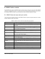
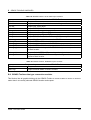
B. GRASS Toolbox modules
B.1. GRASS Toolbox data import and export modules . . . . . . .
B.2. GRASS Toolbox data type conversion modules . . . . . . . .
B.3. GRASS Toolbox region and projection configuration modules
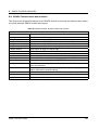
B.4. GRASS Toolbox raster data modules . . . . . . . . . . . . . .
B.5. GRASS Toolbox vector data modules . . . . . . . . . . . . .
B.6. GRASS Toolbox imagery data modules . . . . . . . . . . . .
B.7. GRASS Toolbox database modules . . . . . . . . . . . . . . .
B.8. GRASS Toolbox 3D modules . . . . . . . . . . . . . . . . . .
B.9. GRASS Toolbox help modules . . . . . . . . . . . . . . . . .
C. GNU General Public License
C.1. Quantum GIS Qt exception for GPL
.
.
.
.
.
.
.
.
.
.
.
.
.
.
.
.
.
.
.
.
.
.
.
.
.
.
.
.
.
.
.
.
.
.
.
.
.
.
.
.
.
.
.
.
.
.
.
.
.
.
.
.
.
.
.
.
.
.
.
.
.
.
.
.
.
.
.
.
.
.
.
.
.
.
.
.
.
.
.
.
.
.
.
.
.
.
.
.
.
.
.
.
.
.
.
.
.
.
.
.
.
.
.
.
.
.
.
.
.
.
.
.
.
.
.
.
.
.
.
.
.
.
.
.
.
.
221
221
222
223
226
232
235
236
237
237
238
. . . . . . . . . . . . . . . . . . . . . . . . . . . . 243
D. GNU Free Documentation License
244
Cited literature
253
QGIS 1.4.0 User Guide
ix
List of Figures
List of Figures
1.
2.
3.
4.
5.
6.
7.
8.
9.
10.
11.
12.
13.
14.
15.
16.
17.
18.
19.
20.
21.
22.
23.
24.
25.
26.
27.
28.
29.
30.
31.
32.
33.
34.
35.
36.
37.
38.
39.
40.
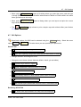
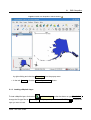
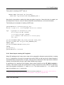
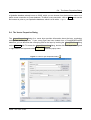
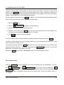
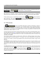
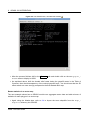
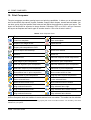
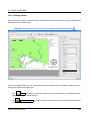
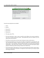
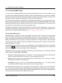
A Simple QGIS Session
. . . . . . . . . . . . . . . . . . . . . . . . . . . . .
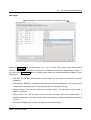
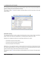
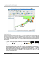
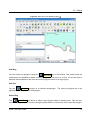
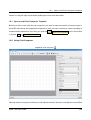
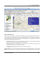
QGIS GUI with Alaska sample data (KDE) . . . . . . . . . . . . . . . . . . . .
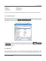
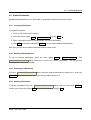
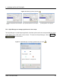
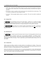
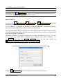
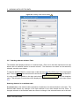
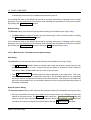
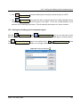
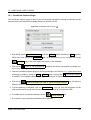
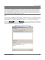
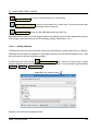
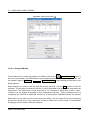
Define shortcut options (KDE) . . . . . . . . . . . . . . . . . . . . . . . . . .
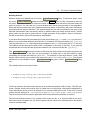
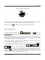
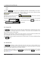
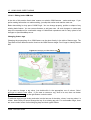
Measure tools in action
. . . . . . . . . . . . . . . . . . . . . . . . . . . . . .
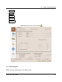
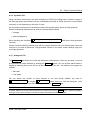
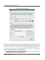
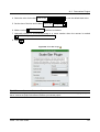
Proxy-settings in QGIS
. . . . . . . . . . . . . . . . . . . . . . . . . . . . . .
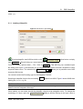
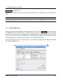
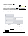
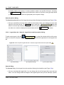
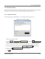
Add Vector Layer Dialog
. . . . . . . . . . . . . . . . . . . . . . . . . . . . .
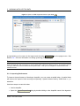
Open an OGR Supported Vector Layer Dialog
. . . . . . . . . . . . . . . . .
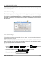
QGIS with Shapefile of Alaska loaded
. . . . . . . . . . . . . . . . . . . . . .
◦
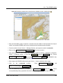
Map in lat/lon crossing the 180 longitude line
. . . . . . . . . . . . . . . . .
◦
Map crossing 180 longitude applying the ST_Shift_Longitude function
. . .
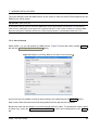
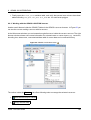
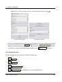
Vector Layer Properties Dialog
. . . . . . . . . . . . . . . . . . . . . . . . . .
Symbolizing Options
. . . . . . . . . . . . . . . . . . . . . . . . . . . . . . .
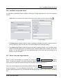
New Single Symbolizing options
. . . . . . . . . . . . . . . . . . . . . . . . .
New Categorized Symbolizing options . . . . . . . . . . . . . . . . . . . . . .
New Graduated Symbolizing options
. . . . . . . . . . . . . . . . . . . . . .
Defining symbol properties
. . . . . . . . . . . . . . . . . . . . . . . . . . . .
Style Manager to manage symbols and color ramps
. . . . . . . . . . . . . .
Dialog to select an edit widget for an attribute column
. . . . . . . . . . . . .
Select feature and choose action
. . . . . . . . . . . . . . . . . . . . . . . .
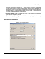
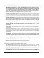
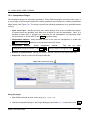
Vector properties dialog with diagram tab
. . . . . . . . . . . . . . . . . . . .
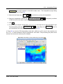
Diagram from temperature data overlayed on a map
. . . . . . . . . . . . . .
Edit snapping options on a layer basis . . . . . . . . . . . . . . . . . . . . . .
Enter Attribute Values Dialog after digitizing a new vector feature . . . . . . .
Redo and Undo digitizing steps
. . . . . . . . . . . . . . . . . . . . . . . . .
Rotate Point Symbols
. . . . . . . . . . . . . . . . . . . . . . . . . . . . . . .
Creating a New Vector Dialog
. . . . . . . . . . . . . . . . . . . . . . . . . .
Attribute Table for Alaska layer
. . . . . . . . . . . . . . . . . . . . . . . . . .
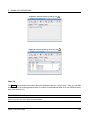
Query Builder
. . . . . . . . . . . . . . . . . . . . . . . . . . . . . . . . . . .
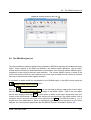
Field Calculator
. . . . . . . . . . . . . . . . . . . . . . . . . . . . . . . . . .
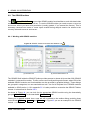
Raster Layers Properties Dialog
. . . . . . . . . . . . . . . . . . . . . . . . .
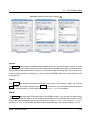
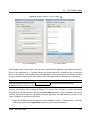
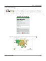
Dialog for adding a WMS server, showing its available layers
. . . . . . . . .
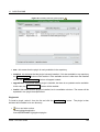
Dialog for searching WMS servers after some keywords . . . . . . . . . . . .
Adding a WFS layer
. . . . . . . . . . . . . . . . . . . . . . . . . . . . . . . .
CRS tab in the QGIS Options Dialog
. . . . . . . . . . . . . . . . . . . . . .
Projection Dialog
. . . . . . . . . . . . . . . . . . . . . . . . . . . . . . . . .
Custom CRS Dialog
. . . . . . . . . . . . . . . . . . . . . . . . . . . . . . . .
GRASS data in the alaska LOCATION (adapted from Neteler & Mitasova 2008)
Creating a new GRASS LOCATION or a new MAPSET in QGIS
. . . . . . .
GRASS Digitizing Toolbar
. . . . . . . . . . . . . . . . . . . . . . . . . . . .
GRASS Digitizing Category Tab
. . . . . . . . . . . . . . . . . . . . . . . . .
QGIS 1.4.0 User Guide
.
.
.
.
.
.
.
.
.
.
.
.
.
.
.
.
.
.
.
.
.
.
.
.
.
.
.
.
.
.
.
.
.
.
.
.
.
.
.
.
.
.
.
.
.
.
.
.
.
.
.
.
.
.
.
.
.
.
.
.
.
.
.
.
.
.
.
.
.
.
.
.
.
.
.
.
.
.
.
.
.
.
.
.
.
.
.
.
.
.
.
.
.
.
.
.
.
.
.
.
.
.
.
.
.
.
.
.
.
. . .
. . .
. . .
.
.
.
.
.
.
.
.
.
.
.
.
.
.
.
.
.
.
.
.
.
.
.
.
.
.
.
.
.
.
.
.
.
.
.
.
.
.
.
.
14
18
19
29
34
37
38
39
46
46
47
49
51
52
53
54
54
57
61
63
64
65
68
73
75
76
77
79
81
85
92
94
98
101
103
104
108
109
114
115
x
List of Figures
41.
42.
43.
44.
45.
46.
47.
48.
49.
50.
51.
52.
53.
54.
55.
56.
57.
58.
59.
60.
61.
62.
63.
64.
65.
66.
67.
68.
69.
70.
71.
72.
73.
74.
75.
76.
77.
78.
79.
80.
81.
82.
GRASS Digitizing Settings Tab
. . . . . . . . . . . . . . . . . . . . . . . . . . . .
GRASS Digitizing Symbolog Tab . . . . . . . . . . . . . . . . . . . . . . . . . . .
GRASS Digitizing Table Tab
. . . . . . . . . . . . . . . . . . . . . . . . . . . . .
GRASS Toolbox and searchable Modules List
. . . . . . . . . . . . . . . . . . .
GRASS Toolbox Module Dialogs
. . . . . . . . . . . . . . . . . . . . . . . . . . .
GRASS Toolbox r.contour module
. . . . . . . . . . . . . . . . . . . . . . . . . .
GRASS module v.generalize to smooth a vector map
. . . . . . . . . . . . . . .
The GRASS shell, r.shaded.relief module
. . . . . . . . . . . . . . . . . . . . . .
Displaying shaded relief created with the GRASS module r.shaded.relief
. . . .
GRASS LOCATION browser
. . . . . . . . . . . . . . . . . . . . . . . . . . . . .
Print Composer
. . . . . . . . . . . . . . . . . . . . . . . . . . . . . . . . . . . .
Print Composer map item tab - Map and Extents dialog
. . . . . . . . . . . . . .
Print Composer map item tab - Grid and General options dialog
. . . . . . . . .
Print composer label item tab - Label options and General options dialog
. . . .
Print composer image item tab - Picture options and General options
. . . . . .
Print composer legend item tab - General, Legend items and Item option dialog .
Print composer scalebar item tab - Scalebar and General options dialog
. . . .
Print composer basic shape and arrow item tab - Shape and Arrow options dialog
Print Composer with map view, legend, scalebar, coordinates and text added . .
Composer Manager
. . . . . . . . . . . . . . . . . . . . . . . . . . . . . . . . . .
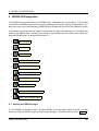
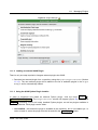
Plugin Manager
. . . . . . . . . . . . . . . . . . . . . . . . . . . . . . . . . . . .
Installing external python plugins . . . . . . . . . . . . . . . . . . . . . . . . . . .
Coordinate Cature Plugin
. . . . . . . . . . . . . . . . . . . . . . . . . . . . . . .
Copyright Label Plugin
. . . . . . . . . . . . . . . . . . . . . . . . . . . . . . . .
North Arrow Plugin
. . . . . . . . . . . . . . . . . . . . . . . . . . . . . . . . . .
Scale Bar Plugin
. . . . . . . . . . . . . . . . . . . . . . . . . . . . . . . . . . . .
Delimited Text Dialog
. . . . . . . . . . . . . . . . . . . . . . . . . . . . . . . . .
Dxf2Shape Converter Plugin
. . . . . . . . . . . . . . . . . . . . . . . . . . . . .
The eVis display window
. . . . . . . . . . . . . . . . . . . . . . . . . . . . . . .
The eVis Options window . . . . . . . . . . . . . . . . . . . . . . . . . . . . . . .
The eVis External Applications window
. . . . . . . . . . . . . . . . . . . . . . .
The eVis Database connection window
. . . . . . . . . . . . . . . . . . . . . . .
The eVis SQL query tab
. . . . . . . . . . . . . . . . . . . . . . . . . . . . . . .
The eVis Perdefined queries tab
. . . . . . . . . . . . . . . . . . . . . . . . . . .
Georeferencer Plugin Dialog
. . . . . . . . . . . . . . . . . . . . . . . . . . . . .
Add points to the raster image
. . . . . . . . . . . . . . . . . . . . . . . . . . . .
The GPS Tools dialog window
. . . . . . . . . . . . . . . . . . . . . . . . . . . .
The download tool
. . . . . . . . . . . . . . . . . . . . . . . . . . . . . . . . . . .
Interpolation Plugin
. . . . . . . . . . . . . . . . . . . . . . . . . . . . . . . . . .
Interpolation of elevp data using TIN method
. . . . . . . . . . . . . . . . . . . .
Smart labeling of vector point layers
. . . . . . . . . . . . . . . . . . . . . . . . .
Smart labeling of vector line layers . . . . . . . . . . . . . . . . . . . . . . . . . .
QGIS 1.4.0 User Guide
.
.
.
.
.
.
.
.
.
.
.
.
.
.
.
.
.
.
.
.
.
.
.
.
.
.
.
.
.
.
.
.
.
.
.
.
.
.
.
.
.
.
.
.
.
.
.
.
.
.
.
.
.
.
.
.
.
.
.
.
.
.
.
.
.
.
.
.
.
.
.
.
.
.
.
.
.
.
.
.
.
.
.
116
116
117
118
119
121
122
124
125
126
129
131
133
134
135
136
138
139
140
141
143
144
148
149
150
151
153
154
156
157
159
162
164
165
173
174
177
178
180
181
182
183
xi
List of Figures
83.
84.
85.
86.
87.
88.
89.
90.
91.
92.
93.
94.
95.
96.
97.
98.
99.
100.
101.
102.
103.
Smart labeling of vector polygon layers
. . . . . . . . . . . . . .
Dialog to change label engine settings
. . . . . . . . . . . . . .
Arrange raster and vector layers for QGIS project file
. . . . . .
Export to MapServer Dialog
. . . . . . . . . . . . . . . . . . . .
Test PNG created by shp2img with all MapServer Export layers
OGR Layer Converter Plugin
. . . . . . . . . . . . . . . . . . . .
Create Oracle connection dialog
. . . . . . . . . . . . . . . . . .
Select Oracle GeoRaster dialog
. . . . . . . . . . . . . . . . . .
OpenStreetMap data in the web
. . . . . . . . . . . . . . . . . .
OSM plugin user interface
. . . . . . . . . . . . . . . . . . . . .
Load OSM data dialog
. . . . . . . . . . . . . . . . . . . . . . .
Changing an OSM feature tag
. . . . . . . . . . . . . . . . . . .
OSM point creation message . . . . . . . . . . . . . . . . . . . .
OSM download dialog . . . . . . . . . . . . . . . . . . . . . . . .
OSM upload dialog
. . . . . . . . . . . . . . . . . . . . . . . . .
OSM saving dialog
. . . . . . . . . . . . . . . . . . . . . . . . .
OSM import message dialog
. . . . . . . . . . . . . . . . . . . .
Import data to OSM dialog
. . . . . . . . . . . . . . . . . . . . .
Raster Terrain Modelling Plugin
. . . . . . . . . . . . . . . . . .
Quick Print Dialog
. . . . . . . . . . . . . . . . . . . . . . . . . .
Quick Print result as DIN A4 PDF using the alaska sample dataset
QGIS 1.4.0 User Guide
.
.
.
.
.
.
.
.
.
.
.
.
.
.
.
.
.
.
.
.
.
.
.
.
.
.
.
.
.
.
.
.
.
.
.
.
.
.
.
.
.
.
.
.
.
.
.
.
.
.
.
.
.
.
.
.
.
.
.
.
.
.
.
.
.
.
.
.
.
.
.
.
.
.
.
.
.
.
.
.
.
.
.
.
.
.
.
.
.
.
.
.
.
.
.
.
.
.
.
.
.
.
.
.
.
.
.
.
.
.
.
.
.
.
.
.
.
.
.
.
.
.
.
.
.
.
.
.
.
.
.
.
.
.
.
.
.
.
.
.
.
.
.
.
.
.
.
.
.
.
.
.
.
.
.
.
.
.
.
.
.
.
.
.
.
.
.
.
.
.
.
.
.
.
.
.
.
.
.
.
.
.
.
.
.
.
.
.
.
.
.
.
.
.
.
.
.
.
.
.
.
.
.
.
.
.
.
.
.
.
.
.
.
.
.
.
.
.
.
.
.
.
.
.
.
.
.
.
.
.
183
184
185
186
188
189
192
193
195
197
198
200
201
204
206
207
207
208
209
211
211
xii
List of Tables
List of Tables
1.
2.
3.
4.
5.
6.
7.
8.
9.
10.
11.
12.
13.
14.
15.
16.
17.
18.
19.
20.
21.
22.
23.
24.
25.
26.
27.
28.
29.
30.
31.
32.
33.
34.
35.
36.
37.
38.
39.
40.
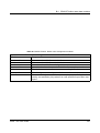
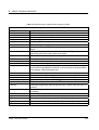
PostGIS Connection Parameters . . . . . . . . . . . . . . . . . . . .
Vector layer basic editing toolbar . . . . . . . . . . . . . . . . . . . .
Vector layer advanced editing toolbar . . . . . . . . . . . . . . . . . .
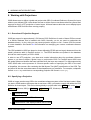
WMS Connection Parameters . . . . . . . . . . . . . . . . . . . . . .
GRASS Digitizing Tools . . . . . . . . . . . . . . . . . . . . . . . . .
Print Composer Tools . . . . . . . . . . . . . . . . . . . . . . . . . .
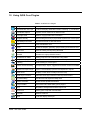
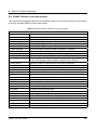
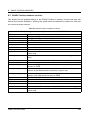
23 QGIS Core Plugins . . . . . . . . . . . . . . . . . . . . . . . . . .
Example format using absolute path, relative path, and a URL . . . .
The XML tags read by eVis . . . . . . . . . . . . . . . . . . . . . . .
fTools Analysis tools . . . . . . . . . . . . . . . . . . . . . . . . . . .
fTools Research tools . . . . . . . . . . . . . . . . . . . . . . . . . .
fTools Geoprocessing tools . . . . . . . . . . . . . . . . . . . . . . .
fTools Geometry tools . . . . . . . . . . . . . . . . . . . . . . . . . .
fTools Data management tools . . . . . . . . . . . . . . . . . . . . .
Other Core Plugins . . . . . . . . . . . . . . . . . . . . . . . . . . . .
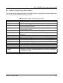
Current moderated external QGIS Plugins . . . . . . . . . . . . . . .
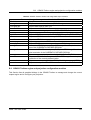
GRASS Toolbox: Raster and Image data import modules . . . . . .
GRASS Toolbox: Vector data import modules . . . . . . . . . . . . .
GRASS Toolbox: Database import modules . . . . . . . . . . . . . .
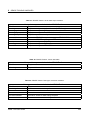
GRASS Toolbox: Raster and Image data export modules . . . . . .
GRASS Toolbox: Vector data export modules . . . . . . . . . . . . .
GRASS Toolbox: Vector data table . . . . . . . . . . . . . . . . . . .
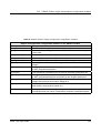
GRASS Toolbox: Data type conversion modules . . . . . . . . . . .
GRASS Toolbox: Region and projection configuration modules . . .
GRASS Toolbox: Develop raster map modules . . . . . . . . . . . .
GRASS Toolbox: Raster color management modules . . . . . . . . .
GRASS Toolbox: Spatial raster analysis modules . . . . . . . . . . .
GRASS Toolbox: Hydrologic modelling modules . . . . . . . . . . .
GRASS Toolbox: Change raster category values and labels modules
GRASS Toolbox: Surface management modules . . . . . . . . . . .
GRASS Toolbox: Reports and statistic analysis modules . . . . . . .
GRASS Toolbox: Develop vector map modules . . . . . . . . . . . .
GRASS Toolbox: Database connection modules . . . . . . . . . . .
GRASS Toolbox: Spatial vector and network analysis modules . . .
GRASS Toolbox: Change vector field modules . . . . . . . . . . . .
GRASS Toolbox: Working with vector points modules . . . . . . . .
GRASS Toolbox: Vector update by other maps modules . . . . . . .
GRASS Toolbox: Vector report and statistic modules . . . . . . . . .
GRASS Toolbox: Imagery analysis modules . . . . . . . . . . . . . .
GRASS Toolbox: Database modules . . . . . . . . . . . . . . . . . .
QGIS 1.4.0 User Guide
.
.
.
.
.
.
.
.
.
.
.
.
.
.
.
.
.
.
.
.
.
.
.
.
.
.
.
.
.
.
.
.
.
.
.
.
.
.
.
.
.
.
.
.
.
.
.
.
.
.
.
.
.
.
.
.
.
.
.
.
.
.
.
.
.
.
.
.
.
.
.
.
.
.
.
.
.
.
.
.
.
.
.
.
.
.
.
.
.
.
.
.
.
.
.
.
.
.
.
.
.
.
.
.
.
.
.
.
.
.
.
.
.
.
.
.
.
.
.
.
.
.
.
.
.
.
.
.
.
.
.
.
.
.
.
.
.
.
.
.
.
.
.
.
.
.
.
.
.
.
.
.
.
.
.
.
.
.
.
.
.
.
.
.
.
.
.
.
.
.
.
.
.
.
.
.
.
.
.
.
.
.
.
.
.
.
.
.
.
.
.
.
.
.
.
.
.
.
.
.
.
.
.
.
.
.
.
.
.
.
.
.
.
.
.
.
.
.
.
.
.
.
.
.
.
.
.
.
.
.
.
.
.
.
.
.
.
.
.
.
.
.
.
.
.
.
.
.
.
.
.
.
.
.
.
.
.
.
.
.
.
.
.
.
.
.
.
.
.
.
.
.
.
.
.
.
.
.
.
.
.
.
.
.
.
.
.
.
.
.
.
.
.
.
.
.
.
.
.
.
.
.
.
.
.
.
.
.
.
.
.
.
.
.
.
.
.
.
.
.
.
.
.
.
.
.
.
.
.
.
.
.
.
.
.
.
.
.
.
.
.
.
.
.
.
.
.
.
.
.
.
.
.
.
.
.
.
.
.
.
.
.
.
.
.
.
.
.
.
.
.
.
.
.
.
.
.
.
.
.
.
.
.
.
.
.
.
.
.
.
.
.
.
.
.
.
.
.
.
.
41
67
72
91
114
128
147
159
166
169
170
170
171
171
212
213
221
222
222
223
224
224
224
225
226
227
228
229
229
230
231
232
233
233
233
234
234
234
235
236
xiii
List of Tables
41. GRASS Toolbox: 3D Visualization . . . . . . . . . . . . . . . . . . . . . . . . . . . . . 237
42. GRASS Toolbox: Reference Manual . . . . . . . . . . . . . . . . . . . . . . . . . . . . 237
QGIS 1.4.0 User Guide
xiv
QGIS Tips
QGIS Tips
1.
2.
3.
4.
5.
6.
7.
8.
9.
10.
11.
12.
13.
14.
15.
16.
17.
18.
19.
20.
21.
22.
23.
24.
25.
26.
27.
28.
29.
30.
31.
32.
33.
34.
35.
36.
37.
38.
39.
40.
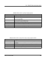
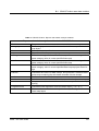
U P - TO - DATE D OCUMENTATION . . . . . . . . . . . . . . . . . . . . . . . .
E XAMPLE U SING COMMAND LINE ARGUMENTS . . . . . . . . . . . . . . .
R ESTORING TOOLBARS . . . . . . . . . . . . . . . . . . . . . . . . . . . .
Z OOMING THE M AP WITH THE M OUSE W HEEL . . . . . . . . . . . . . . .
PANNING THE M AP WITH THE A RROW K EYS AND S PACE B AR . . . . . . .
C ALCULATING THE CORRECT S CALE OF YOUR M AP C ANVAS . . . . . . .
U SING P ROXIES . . . . . . . . . . . . . . . . . . . . . . . . . . . . . . . .
L AYER C OLORS . . . . . . . . . . . . . . . . . . . . . . . . . . . . . . . . .
L OAD LAYER AND PROJECT FROM MOUNTED EXTERNAL DRIVES ON OS X
QGIS U SER S ETTINGS AND S ECURITY . . . . . . . . . . . . . . . . . . .
P OST GIS L AYERS . . . . . . . . . . . . . . . . . . . . . . . . . . . . . . .
E XPORTING DATASETS FROM P OST GIS . . . . . . . . . . . . . . . . . . .
I MPORTING S HAPEFILES C ONTAINING P OSTGRE SQL R ESERVED W ORDS
C ONCURRENT E DITS . . . . . . . . . . . . . . . . . . . . . . . . . . . . . .
S AVE R EGULARLY . . . . . . . . . . . . . . . . . . . . . . . . . . . . . . .
ATTRIBUTE VALUE T YPES . . . . . . . . . . . . . . . . . . . . . . . . . . .
V ERTEX M ARKERS . . . . . . . . . . . . . . . . . . . . . . . . . . . . . . .
C ONGRUENCY OF PASTED F EATURES . . . . . . . . . . . . . . . . . . . .
F EATURE D ELETION S UPPORT . . . . . . . . . . . . . . . . . . . . . . . .
DATA I NTEGRITY . . . . . . . . . . . . . . . . . . . . . . . . . . . . . . . .
M ANIPULATING ATTRIBUTE DATA . . . . . . . . . . . . . . . . . . . . . . .
C HANGING THE L AYER D EFINITION . . . . . . . . . . . . . . . . . . . . . .
V IEWING A S INGLE B AND OF A M ULTIBAND R ASTER . . . . . . . . . . . .
G ATHERING R ASTER S TATISTICS . . . . . . . . . . . . . . . . . . . . . . .
O N WMS S ERVER URL S . . . . . . . . . . . . . . . . . . . . . . . . . . .
I MAGE E NCODING . . . . . . . . . . . . . . . . . . . . . . . . . . . . . . .
WMS L AYER O RDERING . . . . . . . . . . . . . . . . . . . . . . . . . . . .
WMS L AYER T RANSPARENCY . . . . . . . . . . . . . . . . . . . . . . . . .
WMS P ROJECTIONS . . . . . . . . . . . . . . . . . . . . . . . . . . . . . .
ACCESSING SECURED OGC- LAYERS . . . . . . . . . . . . . . . . . . . . .
F INDING WFS S ERVERS . . . . . . . . . . . . . . . . . . . . . . . . . . . .
ACCESSING SECURE WFS S ERVERS . . . . . . . . . . . . . . . . . . . . .
P ROJECT P ROPERTIES D IALOG . . . . . . . . . . . . . . . . . . . . . . . .
GRASS DATA L OADING . . . . . . . . . . . . . . . . . . . . . . . . . . . .
L EARNING THE GRASS V ECTOR M ODEL . . . . . . . . . . . . . . . . . .
C REATING AN ATTRIBUTE TABLE FOR A NEW GRASS VECTOR LAYER . . .
D IGITIZING POLYGONES IN GRASS . . . . . . . . . . . . . . . . . . . . .
C REATING AN ADDITIONAL GRASS ’ LAYER ’ WITH QGIS . . . . . . . . . .
GRASS E DIT P ERMISSIONS . . . . . . . . . . . . . . . . . . . . . . . . .
D ISPLAY RESULTS IMMEDIATELY . . . . . . . . . . . . . . . . . . . . . . . .
QGIS 1.4.0 User Guide
.
.
.
.
.
.
.
.
.
.
.
.
.
.
.
.
.
.
.
.
.
.
.
.
.
.
.
.
.
.
.
.
.
.
.
.
.
.
.
.
.
.
.
.
.
.
.
.
.
.
.
.
.
.
.
.
.
.
.
.
.
.
.
.
.
.
.
.
.
.
.
.
.
.
.
.
.
.
.
.
.
.
.
.
.
.
.
.
.
.
.
.
.
.
.
.
.
.
.
.
.
.
.
.
.
.
.
.
.
.
.
.
.
.
.
.
.
.
.
.
.
.
.
.
.
.
.
.
.
.
.
.
.
.
.
.
.
.
.
.
.
.
.
.
.
.
.
.
.
.
.
.
.
.
.
.
.
.
.
.
.
.
.
.
.
.
.
.
.
.
.
.
.
.
.
.
.
.
.
.
.
.
.
.
.
.
.
.
.
.
.
.
.
.
.
.
.
.
.
.
.
.
.
.
.
.
.
.
.
.
.
.
.
.
.
.
.
.
.
.
.
.
.
.
.
.
.
.
.
.
.
.
.
.
.
.
.
.
.
.
.
.
.
.
.
.
.
.
.
.
.
.
.
.
.
.
.
.
.
.
.
.
.
.
.
.
.
.
.
.
.
.
.
.
.
.
.
.
.
.
1
17
23
25
26
27
34
37
38
41
42
43
44
63
68
69
69
71
71
71
78
80
86
89
92
93
93
93
94
97
99
99
102
108
113
113
113
115
116
120
xv
QGIS Tips
41.
42.
43.
44.
45.
46.
47.
48.
T HE SIMPLIFY TOOL . . . . . . . . . . . . . . . .
OTHER USES FOR R . CONTOUR . . . . . . . . . .
C RASHING P LUGINS . . . . . . . . . . . . . . . .
U SING EXPERIMENTAL PLUGINS . . . . . . . . . .
P LUGINS S ETTINGS S AVED TO P ROJECT . . . .
C REATING A VECTOR LAYER FROM A M ICROSOFT
C HOOSING THE RESAMPLING METHOD . . . . . .
A DD MORE REPOSITORIES . . . . . . . . . . . . .
QGIS 1.4.0 User Guide
. . . . . . . . . . . .
. . . . . . . . . . . .
. . . . . . . . . . . .
. . . . . . . . . . . .
. . . . . . . . . . . .
E XCEL W ORKSHEET
. . . . . . . . . . . .
. . . . . . . . . . . .
.
.
.
.
.
.
.
.
.
.
.
.
.
.
.
.
.
.
.
.
.
.
.
.
.
.
.
.
.
.
.
.
.
.
.
.
.
.
.
.
.
.
.
.
.
.
.
.
.
.
.
.
.
.
.
.
.
.
.
.
.
.
.
.
.
.
.
.
.
.
.
.
121
122
142
146
151
165
175
213
xvi
1. Foreword
Welcome to the wonderful world of Geographical Information Systems (GIS)! Quantum GIS (QGIS)
is an Open Source Geographic Information System. The project was born in May of 2002 and was
established as a project on SourceForge in June of the same year. We’ve worked hard to make
GIS software (which is traditionally expensive proprietary software) a viable prospect for anyone with
basic access to a Personal Computer. QGIS currently runs on most Unix platforms, Windows, and
OS X. QGIS is developed using the Qt toolkit (http://www.trolltech.com) and C++. This means
that QGIS feels snappy to use and has a pleasing, easy-to- use graphical user interface (GUI).
QGIS aims to be an easy-to-use GIS, providing common functions and features. The initial goal was
to provide a GIS data viewer. QGIS has reached the point in its evolution where it is being used
by many for their daily GIS data viewing needs. QGIS supports a number of raster and vector data
formats, with new format support easily added using the plugin architecture (see Appendix A for a full
list of currently supported data formats).
QGIS is released under the GNU General Public License (GPL). Developing QGIS under this license
means that you can inspect and modify the source code, and guarantees that you, our happy user,
will always have access to a GIS program that is free of cost and can be freely modified. You should
have received a full copy of the license with your copy of QGIS, and you also can find it in Appendix
C.
Tip 1 U P - TO - DATE D OCUMENTATION
The latest version of this document can always be found at http://download.osgeo.org/qgis/doc/manual/,
or in the documentation area of the QGIS website at http://qgis.osgeo.org/documentation/
1.1. Features
QGIS offers many common GIS functionalities provided by core features and plugins. As a short
summary they are presented in six categories to gain a first insight.
View data
You can view and overlay vector and raster data in different formats and projections without conversion to an internal or common format. Supported formats include:
• spatially-enabled PostgreSQL tables using PostGIS, vector formats supported by the installed
OGR library, including ESRI shapefiles, MapInfo, SDTS and GML (see Appendix A.1 for the
complete list) .
• Raster and imagery formats supported by the installed GDAL (Geospatial Data Abstraction
Library) library, such as GeoTiff, Erdas Img., ArcInfo Ascii Grid, JPEG, PNG (see Appendix A.2
QGIS 1.4.0 User Guide
1
1 FOREWORD
for the complete list).
• SpatiaLite databases (see Section 5.3)
• GRASS raster and vector data from GRASS databases (location/mapset),
• Online spatial data served as OGC-compliant Web Map Service (WMS) or Web Feature Service
(WFS),
• OpenStreetMap data.
Explore data and compose maps
You can compose maps and interactively explore spatial data with a friendly GUI. The many helpful
tools available in the GUI include:
• on the fly projection
• map composer
• overview panel
• spatial bookmarks
• identify/select features
• edit/view/search attributes
• feature labeling
• change vector and raster symbology
• add a graticule layer now via fTools plugin
• decorate your map with a north arrow scale bar and copyright label
• save and restore projects
Create, edit, manage and export data
You can create, edit, manage and export vector maps in several formats. Raster data have to be
imported into GRASS to be able to edit and export them into other formats. QGIS offers the following:
• digitizing tools for OGR supported formats and GRASS vector layer
• create and edit shapefiles and GRASS vector layers
• geocode images with the Georeferencer plugin
• GPS tools to import and export GPX format, and convert other GPS formats to GPX or
QGIS 1.4.0 User Guide
2
1.1 Features
down/upload directly to a GPS unit (on Linux, usb: has been added to list of GPS devices)
• visualize and edit OpenStreetMap data
• create PostGIS layers from shapefiles with the SPIT plugin
• improved handling of PostGIS tables
• manage vector attribute tables with the new attribute table (see Section 5.5.7) or Table Manager
plugin
• save screenshots as georeferenced images
Analyse data
You can perform spatial data analysis on PostgreSQL/PostGIS and other OGR supported formats
using the fTools python plugin. QGIS currently offers vector analysis, sampling, geoprocessing, geometry and database management tools. You can also use the integrated GRASS tools, which
include the complete GRASS functionality of more than 300 modules (See Section 9).
Publish maps on the internet
QGIS can be used to export data to a mapfile and to publish them on the internet using a webserver
with UMN MapServer installed. QGIS can also be used as a WMS or WFS client, and as WMS
server.
Extend QGIS functionality through plugins
QGIS can be adapted to your special needs with the extensible plugin architecture. QGIS provides
libraries that can be used to create plugins. You can even create new applications with C++ or Python!
Core Plugins
1. Add Delimited Text Layer (Loads and displays delimited text files containing x,y coordinates)
2. Coordinate Capture (Capture mouse coordinates in different CRS)
3. Decorations (Copyright Label, North Arrow and Scale bar)
4. Diagram Overlay (Placing diagrams on vector layer)
5. Dxf2Shp Converter (Convert DXF to Shape)
6. GPS Tools (Loading and importing GPS data)
7. GRASS (GRASS GIS integration)
8. Georeferencer GDAL (Adding projection information to raster using GDAL)
QGIS 1.4.0 User Guide
3
1 FOREWORD
9. Interpolation plugin (interpolate based on vertices of a vector layer)
10. Labeling (Smart labeling for vector layers)
11. Mapserver Export (Export QGIS project file to a MapServer map file)
12. OGR Layer Converter (Translate vector layer between formats)
13. OpenStreetMap plugin (Viewer and editor for openstreetmap data)
14. Oracle Spatial GeoRaster support
15. Python Plugin Installer (Download and install QGIS python plugins)
16. Quick Print (Print a map with minimal effort)
17. Raster terrain analysis (Raster based terrain analysis)
18. SPIT (Import Shapefile to PostgreSQL/PostGIS)
19. WFS Plugin (Add WFS layers to QGIS canvas)
20. eVIS (Event Visualization Tool)
21. fTools (Tools for vector data analysis and management)
22. Python Console (Access QGIS environment)
23. Python Plugin Installer
External Python Plugins
QGIS offers a growing number of external python plugins that are provided by the community. These
plugins reside in the official PyQGIS repository, and can be easily installed using the Python Plugin
Installer (See Section 11).
1.1.1. What’s new in version 1.4.0
These are the most relevant additions and improvements:
• Advanced symbology engine (was Symbology-NG branch) in addition to old engine
• Labeling plugin (part of new symbology engine)
• User interface cleanups to copyright, delim text and n-arrow plugins, and map composer interface
• ’Tools’ menu renamed to ’Vector’
QGIS 1.4.0 User Guide
4
1.1 Features
• Added ’newgis’ theme which is a revision by Anita Graser of the original GIS theme by Robert
Szczepanek
• Added ’Configure shortcuts’ dialog
• Added ’Export to PDF’ feature to map composer menu
• Added support to user-specific SVG path in the map composer
• Added ’newgis’ icon theme, a revision of the original ’gis’ theme
• Possibility to add/remove attributes also in attribute table. Small modification to attribute table
such that adding / removing columns is visible
• Field Calculator
• New analysis tools: Zonal statistics, TIN interpolation and Overlay analyzer
QGIS 1.4.0 User Guide
5
1 FOREWORD
1.2. Conventions
This section describes a collection of uniform styles throughout the manual. The conventions used in
this manual are as follows:
GUI Conventions
The GUI convention styles are intended to mimic the appearance of the GUI. In general, the objective
is to use the non-hover appearance, so a user can visually scan the GUI to find something that looks
like the instruction in the manual.
• Menu Options: Layer >
Add a Raster Layer
or
Settings > Toolbars > ⊠ Digitizing
• Tool:
Add a Raster Layer
• Button: Save as Default
• Dialog Box Title: Layer Properties
• Tab: General
• Toolbox Item:
nviz - Open 3D-View in NVIZ
• Checkbox: x Render
• Radio Button: ⊙ Postgis SRID ° EPSG ID
• Select a Number: Hue 60
N
H
• Select a String: Outline style —Solid Line H
• Browse for a File: . . .
• Select a Color: Outline color
• Slider: Transparency 0% ▽
QGIS 1.4.0 User Guide
6
1.2 Conventions
• Input Text: Display Name lakes.shp
A shadow indicates a clickable GUI component.
Text or Keyboard Conventions
The manual also includes styles related to text, keyboard commands and coding to indicate different
entities, such as classes, or methods. They don’t correspond to any actual appearance.
• Hyperlinks: http://qgis.org
¨ ¥
§ ¦
• Single Keystroke: press p
¨
¥
, meaning press and hold the Ctrl key and then press
• Keystroke Combinations: press §Ctrl+B ¦
the B key.
• Name of a File: lakes.shp
• Name of a Class: NewLayer
• Method: classFactory
• Server: myhost.de
• User Text: qgis --help
Code is indicated by a fixed-width font:
PROJCS["NAD_1927_Albers",
GEOGCS["GCS_North_American_1927",
Platform-specific instructions
GUI sequences and small amounts of text can be formatted inline: Click {
File
QGIS} > Quit
to close QGIS. This indicates that on Linux, Unix and Windows platforms, click the File menu option
first, then Quit from the dropdown menu, while on Macintosh OSX platforms, click the QGIS menu
option first, then Quit from the dropdown menu. Larger amounts of text may be formatted as a list:
•
•
•
do this;
do that;
do something else.
or as paragraphs.
QGIS 1.4.0 User Guide
7
1 FOREWORD
Do this and this and this. Then do this and this and this and this and this and this and this
and this and this.
Do that. Then do that and that and that and that and that and that and that and that and that and
that and that and that and that and that and that.
Screenshots that appear throughout the user guide have been created on different platforms; the
platform is indicated by the platform-specific icons at the end of the figure caption.
QGIS 1.4.0 User Guide
8
2. Introduction To GIS
A Geographical Information System (GIS)[? ]1 is a collection of software that allows you to create,
visualize, query and analyze geospatial data. Geospatial data refers to information about the geographic location of an entity. This often involves the use of a geographic coordinate, like a latitude
or longitude value. Spatial data is another commonly used term, as are: geographic data, GIS data,
map data, location data, coordinate data and spatial geometry data.
Applications using geospatial data perform a variety of functions. Map production is the most easily
understood function of geospatial applications. Mapping programs take geospatial data and render
it in a form that is viewable, usually on a computer screen or printed page. Applications can present
static maps (a simple image) or dynamic maps that are customised by the person viewing the map
through a desktop program or a web page.
Many people mistakenly assume that geospatial applications just produce maps, but geospatial data
analysis is another primary function of geospatial applications. Some typical types of analysis include
computing:
1. distances between geographic locations
2. the amount of area (e.g., square meters) within a certain geographic region
3. what geographic features overlap other features
4. the amount of overlap between features
5. the number of locations within a certain distance of another
6. and so on...
These may seem simplistic, but can be applied in all sorts of ways across many disciplines. The results of analysis may be shown on a map, but are often tabulated into a report to support management
decisions.
The recent phenomena of location-based services promises to introduce all sorts of other features,
but many will be based on a combination of maps and analysis. For example, you have a cell phone
that tracks your geographic location. If you have the right software, your phone can tell you what kind
of restaurants are within walking distance. While this is a novel application of geospatial technology,
it is essentially doing geospatial data analysis and listing the results for you.
1
This chapter is by Tyler Mitchell (http://www.oreillynet.com/pub/wlg/7053) and used under the Creative Commons License. Tyler is the author of Web Mapping Illustrated, published by O’Reilly, 2005.
QGIS 1.4.0 User Guide
9
2 INTRODUCTION TO GIS
2.1. Why is all this so new?
Well, it’s not. There are many new hardware devices that are enabling mobile geospatial services.
Many open source geospatial applications are also available, but the existence of geospatially focused hardware and software is nothing new. Global positioning system (GPS) receivers are becoming commonplace, but have been used in various industries for more than a decade. Likewise,
desktop mapping and analysis tools have also been a major commercial market, primarily focused
on industries such as natural resource management.
What is new is how the latest hardware and software is being applied and who is applying it. Traditional users of mapping and analysis tools were highly trained GIS Analysts or digital mapping
technicians trained to use CAD-like tools. Now, the processing capabilities of home PCs and open
source software (OSS) packages have enabled an army of hobbyists, professionals, web developers,
etc. to interact with geospatial data. The learning curve has come down. The costs have come down.
The amount of geospatial technology saturation has increased.
How is geospatial data stored? In a nutshell, there are two types of geospatial data in widespread use
today. This is in addition to traditional tabular data that is also widely used by geospatial applications.
2.1.1. Raster Data
One type of geospatial data is called raster data or simply "a raster". The most easily recognised form
of raster data is digital satellite imagery or air photos. Elevation shading or digital elevation models
are also typically represented as raster data. Any type of map feature can be represented as raster
data, but there are limitations.
A raster is a regular grid made up of cells, or in the case of imagery, pixels. They have a fixed number
of rows and columns. Each cell has a numeric value and has a certain geographic size (e.g. 30x30
meters in size).
Multiple overlapping rasters are used to represent images using more than one colour value (i.e. one
raster for each set of red, green and blue values is combined to create a colour image). Satellite
imagery also represents data in multiple "bands". Each band is essentially a separate, spatially
overlapping raster, where each band holds values of certain wavelengths of light. As you can imagine,
a large raster takes up more file space. A raster with smaller cells can provide more detail, but takes
up more file space. The trick is finding the right balance between cell size for storage purposes and
cell size for analytical or mapping purposes.
QGIS 1.4.0 User Guide
10
2.1 Why is all this so new?
2.1.2. Vector Data
Vector data is also used in geospatial applications. If you stayed awake during trigonometry and
coordinate geometry classes, you will already be familiar with some of the qualities of vector data.
In its simplest sense, vectors are a way of describing a location by using a set of coordinates. Each
coordinate refers to a geographic location using a system of x and y values.
This can be thought of in reference to a Cartesian plane - you know, the diagrams from school
that showed an x and y-axis. You might have used them to chart declining retirement savings or
increasing compound mortgage interest, but the concepts are essential to geospatial data analysis
and mapping.
There are various ways of representing these geographic coordinates depending on your purpose.
This is a whole area of study for another day - map projections.
Vector data takes on three forms, each progressively more complex and building on the former.
1. Points - A single coordinate (x y) represents a discrete geographic location
2. Lines - Multiple coordinates (x1 y1, x2 y2, x3 y4, ... xn yn) strung together in a certain order, like
drawing a line from Point (x1 y1) to Point (x2 y2) and so on. These parts between each point
are considered line segments. They have a length and the line can be said to have a direction
based on the order of the points. Technically, a line is a single pair of coordinates connected
together, whereas a line string is multiple lines connected together.
3. Polygons - When lines are strung together by more than two points, with the last point being at
the same location as the first, we call this a polygon. A triangle, circle, rectangle, etc. are all
polygons. The key feature of polygons is that there is a fixed area within them.
QGIS 1.4.0 User Guide
11
3 GETTING STARTED
3. Getting Started
This chapter gives a quick overview of installing QGIS, some sample data from the QGIS web page
and running a first and simple session visualizing raster and vector layers.
3.1. Installation
Installation of QGIS is very simple. Standard installer packages are available for MS Windows and
Mac OS X. For many flavors of GNU/Linux binary packages (rpm and deb) or software repositories
to add to your installation manager are provided. Get the latest information on binary packages at
the QGIS website at http://qgis.osgeo.org/download/.
Installation from source
If you need to build QGIS from source, please refer to the coding and compiling guide available at
http://qgis.osgeo.org/documentation/. The installation instructions are also distributed with the
QGIS source code.
3.2. Sample Data
The user guide contains examples based on the QGIS sample dataset.
The Windows installer has an option to download the QGIS sample dataset. If checked, the data
will be downloaded to your My Documents folder and placed in a folder called GIS Database. You
may use Windows Explorer to move this folder to any convenient location. If you did not select the
checkbox to install the sample dataset during the initial QGIS installation, you can either
• use GIS data that you already have;
• download the sample data from the QGIS website http://qgis.osgeo.org/download; or
• uninstall QGIS and reinstall with the data download option checked, only if the above solutions
are unsuccessful.
For GNU/Linux and Mac OSX there are not yet dataset installation packages available as rpm,
deb or dmg. To use the sample dataset download the file qgis_sample_data as ZIP or TAR archive
from http://download.osgeo.org/qgis/data/ and unzip or untar the archive on your system. The
Alaska dataset includes all GIS data that are used as examples and screenshots in the user guide,
and also includes a small GRASS database. The projection for the QGIS sample dataset is Alaska
Albers Equal Area with unit feet. The EPSG code is 2964.
PROJCS["Albers Equal Area",
QGIS 1.4.0 User Guide
12
3.3 Sample Session
GEOGCS["NAD27",
DATUM["North_American_Datum_1927",
SPHEROID["Clarke 1866",6378206.4,294.978698213898,
AUTHORITY["EPSG","7008"]],
TOWGS84[-3,142,183,0,0,0,0],
AUTHORITY["EPSG","6267"]],
PRIMEM["Greenwich",0,
AUTHORITY["EPSG","8901"]],
UNIT["degree",0.0174532925199433,
AUTHORITY["EPSG","9108"]],
AUTHORITY["EPSG","4267"]],
PROJECTION["Albers_Conic_Equal_Area"],
PARAMETER["standard_parallel_1",55],
PARAMETER["standard_parallel_2",65],
PARAMETER["latitude_of_center",50],
PARAMETER["longitude_of_center",-154],
PARAMETER["false_easting",0],
PARAMETER["false_northing",0],
UNIT["us_survey_feet",0.3048006096012192]]
If you intend to use QGIS as graphical frontend for GRASS, you can find a selection of sample
locations (e.g. Spearfish or South Dakota) at the official GRASS GIS website
http://grass.osgeo.org/download/data.php.
3.3. Sample Session
Now that you have QGIS installed and a sample dataset available, we would like to demonstrate
a short and simple QGIS sample session. We will visualize a raster and a vector layer. We will
use the landcover raster layer qgis_sample_data/raster/landcover.img and the lakes vector layer
qgis_sample_data/gml/lakes.gml.
start QGIS
•
Start QGIS by typing: qgis at a command prompt, or if using precompiled binary, using the
Applications menu.
•
Start QGIS using the Start menu or desktop shortcut, or double click on a QGIS project file.
•
Double click the icon in your Applications folder.
QGIS 1.4.0 User Guide
13
3 GETTING STARTED
Figure 1: A Simple QGIS Session
Load raster and vector layers from the sample dataset
1. Click on the
Load Raster icon.
2. Browse to the folder qgis_sample_data/raster/, select the ERDAS Img file landcover.img
and click Open .
3. If the file is not listed, check if the Filetype combobox at the bottom of the dialog is set on the
right type, in this case "Erdas Imagine Images (*.img, *.IMG)"
4. Now click on the
Load Vector icon.
5. ⊙ ’File’ should be selected as Source Type in the new Add Vector Layer dialog. Now click
Browse
to select the vector layer.
6. Browse to the folder qgis_sample_data/gml/, select "GML" from the filetype combobox, then
select the GML file lakes.gml and click Open , then in Add Vector dialog click OK .
7. Zoom in a bit to your favorite area with some lakes.
8. Double click the lakes layer in the map legend to open the Layer Properties dialog.
QGIS 1.4.0 User Guide
14
3.3 Sample Session
9. Click on the Symbology
tab and select a blue as fill color.
10. Click on the Labels tab and check the x Display labels checkbox to enable labeling.
Choose NAMES field as Field containing label.
11. To improve readability of labels, you can add a white buffer around them, by clicking “Buffer” in
the list on the left, checking x Buffer labels? and choosing 3 as buffer size.
12. Click Apply , check if the result looks good and finally click OK .
You can see how easy it is to visualize raster and vector layers in QGIS. Let’s move on to the sections
that follow to learn more about the available functionality, features and settings and how to use them.
QGIS 1.4.0 User Guide
15
4 FEATURES AT A GLANCE
4. Features at a Glance
After a first and simple sample session in Section 3 we now want to give you a more detailed overview
of the features of QGIS. Most features presented in the following chapters will be explained and
described in own sections later in the manual.
4.1. Starting and Stopping QGIS
In Section 3.3 you already learned how to start QGIS. We will repeat this here and you will see that
QGIS also provides further command line options.
•
Assuming that QGIS is installed in the PATH, you can start QGIS by typing: qgis at a
command prompt or by double clicking on the QGIS application link (or shortcut) on the desktop
or in the application menu.
•
Start QGIS using the Start menu or desktop shortcut, or double click on a QGIS project file.
•
Double click the icon in your Applications folder. If you need to start QGIS in a shell, run
/path-to-installation-executable/Contents/MacOS/Qgis.
To stop QGIS, click the menu options {
File
¨
¥
QGIS} > Quit, or use the shortcut §Ctrl+Q ¦
.
4.1.1. Command Line Options
QGIS supports a number of options when started from the command line. To get a list of the
options, enter qgis --help on the command line. The usage statement for QGIS is:
qgis --help
Quantum GIS - 1.4.0-Enceladus ’Enceladus’ (exported)
Quantum GIS (QGIS) is a viewer for spatial data sets, including
raster and vector data.
Usage: qgis [options] [FILES]
options:
[--snapshot filename]
emit snapshot of loaded datasets to given file
[--width width]
width of snapshot to emit
[--height height]
height of snapshot to emit
[--lang language]
use language for interface text
[--project projectfile]
load the given QGIS project
[--extent xmin,ymin,xmax,ymax] set initial map extent
[--nologo]
hide splash screen
[--help]
this text
QGIS 1.4.0 User Guide
16
4.1 Starting and Stopping QGIS
FILES:
Files specified on the command line can include rasters,
vectors, and QGIS project files (.qgs):
1. Rasters - Supported formats include GeoTiff, DEM
and others supported by GDAL
2. Vectors - Supported formats include ESRI Shapefiles
and others supported by OGR and PostgreSQL layers using
the PostGIS extension
Tip 2 E XAMPLE U SING
COMMAND LINE ARGUMENTS
You can start QGIS by specifying one or more data files on the command line. For example, assuming you
are in the qgis_sample_data directory, you could start QGIS with a vector layer and a raster file set to load on
startup using the following command: qgis ./raster/landcover.img ./gml/lakes.gml
Command line option --snapshot
This option allows you to create a snapshot in PNG format from the current view. This comes in
handy when you have a lot of projects and want to generate snapshots from your data.
Currently it generates a PNG-file with 800x600 pixels. This can be adapted using the --width and
--height command line arguments. A filename can be added after --snapshot.
Command line option --lang
Based on your locale QGIS, selects the correct localization. If you would like to change your
language, you can specify a language code. For example: --lang=it starts QGIS in italian localization. A list of currently supported languages with language code and status is provided at
http://www.qgis.org/wiki/GUI_Translation_Progress
Command line option --project
Starting QGIS with an existing project file is also possible. Just add the command line option
--project followed by your project name and QGIS will open with all layers loaded described in
the given file.
Command line option --extent
To start with a specific map extent use this option. You need to add the bounding box of your extent
in the following order separated by a comma:
--extent xmin,ymin,xmax,ymax
QGIS 1.4.0 User Guide
17
4 FEATURES AT A GLANCE
Command line option --nologo
This command line argument hides the splash screen when you start QGIS.
4.2. QGIS GUI
When QGIS starts, you are presented with the GUI as shown below (the numbers 1 through 6 in
yellow ovals refer to the six major areas of the interface as discussed below):
Figure 2: QGIS GUI with Alaska sample data
(KDE)
Note: Your window decorations (title bar, etc.) may appear different depending on your operating
system and window manager.
The QGIS GUI is divided into six areas:
QGIS 1.4.0 User Guide
18
4.2 QGIS GUI
1. Menu Bar
2. Tool Bar
3. Map Legend
4. Map View
5. Map Overview
6. Status Bar
These six components of the QGIS interface are described in more detail in the following sections.
4.2.1. Keyboard shortcuts
QGIS provides default keyboard shortcuts for many features. You find them in Section 4.2.2 below. Additionally the menu option Settings > Configure Shortcuts allows to change the default
keyboard shortcuts and to add new keyboard shortcuts to QGIS features.
Figure 3: Define shortcut options
(KDE)
Configuration is very simple. Just select a feature from the list and click on Change , Set none
or Set default . Once you have found your configuration, you can save it as XML file and load it to
another QGIS installation.
4.2.2. Menu Bar
The menu bar provides access to various QGIS features using a standard hierarchical menu. The
top-level menus and a summary of some of the menu options are listed below, together with the icons
QGIS 1.4.0 User Guide
19
4 FEATURES AT A GLANCE
of the corresponding tools as they appear on the toolbar, as well as keyboard shortcuts.2 Although
most menu options have a corresponding tool and vice-versa, the menus are not organized quite like
the toolbars. The toolbar containing the tool is listed after each menu option as a checkbox entry. For
more information about tools and toolbars, see Section 4.2.3.
Menu Option
Shortcut
Reference
Toolbar
¨
¥
Ctrl+N
§
¦
¨
¥
see Section 4.5
⊠ File
see Section 4.5
⊠ File
• File
New Project
Open Project
§Ctrl+O ¦
Open Recent Projects
Save Project
Save Project As
see Section 4.5
¨
¥
Ctrl+S
§
¦
¨
¥
§Ctrl+Shift+S ¦
Save as Image
New Print Composer
⊠ File
see Section 4.5
⊠ File
see Section 4.6
¨
¥
§Ctrl+P ¦
Composer manager
Print Composers
¨
Exit
see Section 4.5
¥
see Section 10
⊠ File
see Section 10
⊠ File
see Section 10
§Ctrl+Q ¦
• Edit
¨
¥
Ctrl+Z ¦
§
¨
see Section 5.5.5
⊠ Advanced Digitizing
see Section 5.5.5
⊠ Advanced Digitizing
see Section 5.5.4
⊠ Digitizing
see Section 5.5.4
⊠ Digitizing
see Section 5.5.4
⊠ Digitizing
Move Feature
see Section 5.5.4
⊠ Digitizing
Delete Selected
Simplify Feature
see Section 5.5.4
⊠ Digitizing
see Section 5.5.5
⊠ Advanced Digitizing
Add Ring
see Section 5.5.5
⊠ Advanced Digitizing
Add Part
Delete Ring
see Section 5.5.5
⊠ Advanced Digitizing
see Section 5.5.5
⊠ Advanced Digitizing
Delete Part
see Section 5.5.5
⊠ Advanced Digitizing
Undo
Redo
Cut Features
Copy Features
Paste Features
¥
Ctrl+Shift+Z
§
¦
¨
¥
Ctrl+X
§
¦
¨
¥
Ctrl+C ¦
§
¨
¥
§Ctrl+V ¦
2
Keyboard shortcuts can now be configured manually (shortcuts presented in this section are the defaults), using the
Configure Shortcuts tool under Settings Menu.
QGIS 1.4.0 User Guide
20
4.2 QGIS GUI
Reshape Features
see Section 5.5.5
⊠ Advanced Digitizing
Split Features
see Section 5.5.5
⊠ Advanced Digitizing
Merge selected Features
see Section 5.5.5
⊠ Advanced Digitizing
Node Tool
Rotate Point Symbols
see Section 5.5.4
⊠ Digitizing
see Section 5.5.5
⊠ Advanced Digitizing
After activating
toogle editing mode for a layer, you will find a capture feature icon in
the Edit menu depending on the layer type (point, line or polygon).
Capture Point
see Section 5.5.4
⊠ Digitizing
Capture Line
see Section 5.5.4
⊠ Digitizing
Capture Polygon
see Section 5.5.4
⊠ Digitizing
• View
⊠ Map Navigation
Pan Map
Zoom In
Zoom Out
¨
¥
Ctrl++
§
¦
¨
¥
⊠ Map Navigation
⊠ Map Navigation
§Ctrl+- ¦
Select Features
Deselect Features
Identify Features
Measure Line
Measure Area
Zoom Full
Zoom To Layer
Zoom To Selection
⊠ Attributes
⊠ Attributes
¤ ¡
£¨I ¢ ¥
⊠ Attributes
M
§
¤ ¡¦
£J ¢¥
¨
⊠ Attributes
⊠ Attributes
⊠ Map Navigation
§F ¦
⊠ Map Navigation
¨
¥
Ctrl+J
§
¦
⊠ Map Navigation
⊠ Map Navigation
Zoom Last
⊠ Map Navigation
Zoom Next
Zoom Actual Size
Map Tips
New Bookmark
Show Bookmarks
Refresh
QGIS 1.4.0 User Guide
¨
¥
Ctrl+B
§
¦
¨ ¥
B
§
¨ ¦
¥
Ctrl+R
§
¦
⊠ Attributes
see Section 4.8
⊠ Attributes
see Section 4.8
⊠ Attributes
⊠ Map Navigation
21
4 FEATURES AT A GLANCE
• Layer
New Vector Layer
Add Vector Layer
Add Raster Layer
Add PostGIS Layer
Add SpatiaLite Layer
Add WMS Layer
¨
¥
Ctrl+Shift+N
§
¦
¥
¨
Ctrl+Shift+V ¦
§
¨
¥
Ctrl+Shift+R
§
¦
¨
¥
see Section 5.5.6
⊠ Manage Layers
see Section 5
⊠ File
see Section 6
⊠ File
Ctrl+Shift+D ¦ see Section 5.2
§
¨
¥
Ctrl+Shift+L
§
¦¥ see Section 5.3
¨
§Ctrl+Shift+W ¦ see Section 7.2
Open Attribute Table
⊠ File
⊠ File
⊠ File
⊠ Attributes
⊠ Digitizing
Toggle editing
Save As Shapefile
Save Selection As Shapefile
¨
¥
§Ctrl+D ¦
⊠ Properties
¥
¨
§Ctrl+Shift+O ¦
⊠ Manage Layers
Remove All From Overview
¨
¥
Hide All Layers
Ctrl+Shift+H
§
¦
⊠ Manage Layers
Show All Layers
⊠ Manage Layers
Remove Layer
Properties
Add to Overview
Add All To Overview
¥
¨
Ctrl+Shift+S
§
¦
• Settings
Panels
Toolbars
Toggle Fullscreen Mode
Project Properties
Custom CRS
Style Manager
¨ ¥
§P ¦
see Section 4.5
see Section 8.4
Configure shortcuts
Options
see Section 4.7
• Plugins - (Futher menu items are added by plugins as they are loaded.)
Manage Plugins
see Section 11.1 ⊠ Plugins
Python Console
QGIS 1.4.0 User Guide
22
4.2 QGIS GUI
• Help
Help Contents
QGIS Home Page
¨ ¥
F1
§
¨ ¦
⊠ Help
¥
§Ctrl+H ¦
Check QGIS Version
About
Note:
The Menu Bar items listed above are the default ones in KDE window manager. In GNOME,
Settings menu is missing and its items are to be found there:
Project Properties
⊠ File menu
Options
⊠ Edit
Custom CRS
⊠ Edit
Panels
⊠ View
Toolbars
Toggle Fullscreen Mode
⊠ View
⊠ View
4.2.3. Toolbars
The toolbars provide access to most of the same functions as the menus, plus additional tools for
interacting with the map. Each toolbar item has popup help available. Hold your mouse over the item
and a short description of the tool’s purpose will be displayed.
Every menubar can be moved around according to your needs. Additionally every menubar can be
switched off using your right mouse button context menu holding the mouse over the toolbars.
Tip 3 R ESTORING
TOOLBARS
If you have accidentally hidden all your toolbars, you can get them back by choosing menu option Settings >
Toolbars .
4.2.4. Map Legend
The map legend area is used to set the visibility and z-ordering of layers. Z-ordering means that
layers listed nearer the top of the legend are drawn over layers listed lower down in the legend. The
checkbox in each legend entry can be used to show or hide the layer.
Layers can be grouped in the legend window by adding a layer group and dragging layers into the
group. To do so, move the mouse pointer to the legend window, right click, choose Add group . A
QGIS 1.4.0 User Guide
23
4 FEATURES AT A GLANCE
new folder appears. Now drag the layers onto to the folder symbol. It is then possible to toggle the
visibility of all the layers in the group with one click. To bring layers out of a group, move the mouse
pointer to the layer symbol, right click, and choose Make to toplevel item . To give the folder a new
name, choose Rename in the right click menu of the group.
The content of the right mouse button context menu depends on whether the loaded legend item you
hold your mouse over is a raster or a vector layer. For GRASS vector layers the toggle editing is
not available. See section 9.7 for information on editing GRASS vector layers.
• Right mouse button menu for raster layers
–
Zoom to layer extent
–
Zoom to best scale (100%)
–
Show in overview
–
Remove
–
Properties
–
Rename
–
Add Group
–
Expand all
–
Collapse all
• Right mouse button menu for vector layers
–
Zoom to layer extent
–
Show in overview
–
Remove
–
Open attribute table
–
Toggle editing (not available for GRASS layers)
–
Save as shapefile
–
Save selection as shapefile
–
Properties
QGIS 1.4.0 User Guide
24
4.2 QGIS GUI
–
Rename
–
Add Group
–
Expand all
–
Collapse all
• Right mouse button menu for layer groups
–
Remove
–
Rename
–
Add Group
–
Expand all
–
Collapse all
If several vector data sources have the same vector type and the same attributes, their symbolisations
may be grouped. This means that if the symbolisation of one data source is changed, the others
automatically have the new symbolisation as well. To group symbologies, open the right click menu
in the legend window and choose Show file groups . The file groups of the layers appear. It is
now possible to drag a file from one file group into another one. If this is done, the symbologies are
grouped. Note that QGIS only permits the drag if the two layers are able to share symbology (same
vector geometry type and same attributes).
4.2.5. Map View
This is the ’business end’ of QGIS - maps are displayed in this area! The map displayed in this
window will depend on the vector and raster layers you have chosen to load (see sections that follow
for more information on how to load layers). The map view can be panned (shifting the focus of the
map display to another region) and zoomed in and out. Various other operations can be performed
on the map as described in the toolbar description above. The map view and the legend are tightly
bound to each other - the maps in view reflect changes you make in the legend area.
Tip 4 Z OOMING
THE
M AP
WITH THE
M OUSE W HEEL
You can use the mouse wheel to zoom in and out on the map. Place the mouse cursor inside the map area
and roll the wheel forward (away from you) to zoom in and backwards (towards you) to zoom out. The mouse
cursor position is the center where the zoom occurs. You can customize the behavior of the mouse wheel
zoom using the Map tools tab under the Settings > Options menu.
QGIS 1.4.0 User Guide
25
4 FEATURES AT A GLANCE
Tip 5 PANNING
THE
M AP
WITH THE
A RROW K EYS
AND
S PACE B AR
You can use the arrow keys to pan in the map. Place the mouse cursor inside the map area and click on the
right arrow key to pan East, left arrow key to pan West, up arrow key to pan North and down arrow key to pan
South. You can also pan the map using the space bar: just move the mouse while holding down space bar.
4.2.6. Map Overview
The map overview panel provides a full extent view of layers added to it. It can be selected under
the menu Settings > Panels . Within the view is a rectangle showing the current map extent. This
allows you to quickly determine which area of the map you are currently viewing. Note that labels
are not rendered to the map overview even if the layers in the map overview have been set up for
labeling.
You can add a single layer to the overview by right-clicking on it in the legend and select
x Show in overview . You can also add layers to, or remove all layers from the overview using
the Overview tools on the toolbar.
If you click and drag the red rectangle in the overview that shows your current extent, the main map
view will update accordingly.
4.2.7. Status Bar
The status bar shows you your current position in map coordinates (e.g. meters or decimal degrees)
as the mouse pointer is moved across the map view. To the left of the coordinate display in the status
bar is a small button that will toggle between showing coordinate position or the view extents of the
map view as you pan and zoom in and out.
A progress bar in the status bar shows progress of rendering as each layer is drawn to the map view.
In some cases, such as the gathering of statistics in raster layers, the progress bar will be used to
show the status of lengthy operations.
If a new plugin or a plugin update is available, you will see a message in the status bar. On the
right side of the status bar is a small checkbox which can be used to temporarily prevent layers being
rendered to the map view (see Section 4.3 below). At the far right of the status bar is a projector icon.
Clicking on this opens the projection properties for the current project.
4.3. Rendering
By default, QGIS renders all visible layers whenever the map canvas must be refreshed. The events
that trigger a refresh of the map canvas include:
QGIS 1.4.0 User Guide
26
4.3 Rendering
Tip 6 C ALCULATING
THE CORRECT
S CALE
OF YOUR
M AP C ANVAS
When you start QGIS, degrees is the default unit, and it tells QGIS that any coordinate in your layer is in
degrees. To get correct scale values, you can either change this to meter manually in the General tab
under Settings > Project Properties or you can select a project Coordinate Reference System (CRS)
projector icon in the lower right-hand corner of the statusbar. In the last case, the units
are set to what the project projection specifies, e.g. ’+units=m’.
clicking on the
• Adding a layer
• Panning or zooming
• Resizing the QGIS window
• Changing the visibility of a layer or layers
QGIS allows you to control the rendering process in a number of ways.
4.3.1. Scale Dependent Rendering
Scale dependent rendering allows you to specify the minimum and maximum scales at which a layer
will be visible. To set scale dependency rendering, open the Properties dialog by double-clicking
on the layer in the legend. On the General
tab, set the minimum and maximum scale values and
then click on the x Use scale dependent rendering checkbox.
You can determine the scale values by first zooming to the level you want to use and noting the scale
value in the QGIS status bar.
4.3.2. Controlling Map Rendering
Map rendering can be controlled in the following ways:
a) Suspending Rendering
To suspend rendering, click the
x Render checkbox in the lower right corner of the statusbar.
When the x Render box is not checked, QGIS does not redraw the canvas in response to any of
the events described in Section 4.3. Examples of when you might want to suspend rendering include:
• Add many layers and symbolize them prior to drawing
• Add one or more large layers and set scale dependency before drawing
QGIS 1.4.0 User Guide
27
4 FEATURES AT A GLANCE
• Add one or more large layers and zoom to a specific view before drawing
• Any combination of the above
Checking the
canvas.
x Render box enables rendering and causes and immediate refresh of the map
b) Setting Layer Add Option
You can set an option to always load new layers without drawing them. This means the layer will
be added to the map, but its visibility checkbox in the legend will be unchecked by default. To set
this option, choose menu option Settings > Options and click on the Rendering & SVG tab.
Uncheck the x By default new layers added to the map should be displayed checkbox. Any layer
added to the map will be off (invisible) by default.
c) Updating the Map Display During Rendering
You can set an option to update the map display as features are drawn. By default, QGIS does
not display any features for a layer until the entire layer has been rendered. To update the display
as features are read from the datastore, choose menu option Settings > Options click on the
Rendering & SVG
tab. Set the feature count to an appropriate value to update the display during
rendering. Setting a value of 0 disables update during drawing (this is the default). Setting a value
too low will result in poor performance as the map canvas is continually updated during the reading
of the features. A suggested value to start with is 500.
d) Influence Rendering Quality
To influence the rendering quality of the map you have 3 options. Choose menu option Settings >
Options click on the Rendering & SVG
tab and select or deselect following checkboxes.
•
x Make lines appear less jagged at the expense of some drawing performance
•
x Fix problems with incorrectly filled polygons
4.4. Measuring
Measuring works within projected coordinate systems only (e.g., UTM). If the loaded map is defined
with a geographic coordinate system (latitude/longitude), the results from line or area measurements
will be incorrect. To fix this you need to set an appropriate map coordinate system (See Section 8).
Both measuring modules also use the snapping settings from the digitizing module. This is useful, if
QGIS 1.4.0 User Guide
28
4.5 Projects
you want to measure along lines or areas in vector layers.
4.4.1. Measure length and areas
QGIS is also able to measure real distances between given points according to a defined ellipsoid. To configure this, choose menu option Settings > Options , click on the Map tools tab
and choose the appropriate ellipsoid. There you can also define a rubberband color and your preferred measurement units (meters or feet). The tool then allows you to click points on the map. Each
segment-length as well as the total shows up in the measure-window. To stop measuring click your
right mouse button.
Areas can also be measured. In the measure window the accumulated area-size appears
In addition, the measuring tool will snap to the currently selected layer, provided that layer has its
snapping tolerance set. (See Section 5.5.1). So if you want to measure exactly along a line feature,
or around a polygon feature, first set its snapping tolerance, then select the layer. Now, when using
the measuring tools, each mouse click (within the tolerance setting) will snap to that layer.
Figure 4: Measure tools in action
(a) Measure lines
(b) Measure areas
4.5. Projects
The state of your QGIS session is considered a Project. QGIS works on one project at a time.
Settings are either considered as being per-project, or as a default for new projects (see Section
4.7). QGIS can save the state of your workspace into a project file using the menu options File >
Save Project or File >
Save Project As .
Load saved projects into a QGIS session using
Open Recent Project .
QGIS 1.4.0 User Guide
>
Open Project
File
>
If you wish to clear your session and start fresh, choose File
>
File
or
29
4 FEATURES AT A GLANCE
New Project . Either of these menu options will prompt you to save the existing project if changes
have been made since it was opened or last saved.
The kinds of information saved in a project file include:
• Layers added
• Layer properties, including symbolization
• Projection for the map view
• Last viewed extent
The project file is saved in XML format, so it is possible to edit the file outside QGIS if you know what
you are doing. The file format was updated several times compared to earlier QGIS versions. Project
files from older QGIS versions may not work properly anymore. To be made aware of this, in the
General tab under Settings > Options you can select
x Promt to save project changes when required
x Warn when opening a project file saved with an older version of QGIS .
Project Properties
In the properties window for the project under
File > Project Properties or
Settings >
Project Properties you set project specific options. These include:
• In the General tab the project title, selection and background color, layer units, precision, and
the option to save relative paths to layers can be defined. In addition the topological editing,
and layerwise snapping options are set here.
• The CRS Coordinate Reference System tab enables you to choose the CRS for this project,
and to enable on-the-fly reprojection of vector layers when displaying layers from a different
CRS.
• With the third Identifiable layers tab you set (or disable) which layers will respond to the
identify tool. (See the Map tools paragraph from the 4.7 section to enable identifying of multiple
layers.)
4.6. Output
There are several ways to generate output from your QGIS session. We have discussed one already
in Section 4.5: saving as a project file. Here is a sampling of other ways to produce output files:
QGIS 1.4.0 User Guide
30
4.7 GUI Options
Save as Image opens a file dialog where you select the name, path and type
• Menu option
of image (PNG or JPG format). A world file with extension PNGW or JPGW saved in the same
folder georeferences the image.
Print Composer opens a dialog where you can layout and print the current
• Menu option
map canvas (see Section 10).
• The
12.16).
Quick Print plugin allows to print a simple map with minimal effort (see Section
4.7. GUI Options
Some basic options for QGIS can be selected using the
option Settings >
Options dialog. Select the menu
Options . The tabs where you can optmize your options are:
General Tab
•
x Promt to save project changes when required
•
x Warn when opening a project file saved with an older version of QGIS
• Change Selection and backgroud Color
• Change the icon theme (choose between default, classic, gis and nkids)
•
x Capitalise layer names in legend
•
x Display classification attribute names in legend
•
x Hide splash screen at startup
•
x Open identify results in a dock window (QGIS restart required)
•
x Open attribute table in a dock window
•
x Add PostGIS layers with double click and select in extended mode
Rendering & SVG Tab
•
x By deafult new layers added to the map should be displayed
QGIS 1.4.0 User Guide
31
4 FEATURES AT A GLANCE
• Define number of features to draw before updating the display.
•
x Use render caching where possible to speed up redraws
•
x Make lines appear less jagged at the expense of some drawing performance
•
x Fix problems with incorrectly filled polygons
•
x Use new generation symbology for rendering
• Add and remove path(s) to search for Scalable Vector Graphics (SVG) symbols
Map tools Tab
• The Mode setting determines which layers will be shown by the Identify tool. By switching to
Top down or Top down, stop at first instead of Current layer attributes for all identifiable
layers (see the Project properties section under: 4.5 to set which layers are identifiable) will be
shown with the Identify tool.
•
x Open feature form, if a single feature is identified
• Define search radius as a percentage of the map width
• Define ellipsoid for distance calculations
• Define rubberband color for measure tools
• Define preferred measurement units (meters or feet)
• Define Mouse wheel action (Zoom, Zoom and recenter, Zoom to mouse cursor, Nothing)
• Define Zoom factor for wheel mouse
Overlay
• Define placement algorithm for labels (choose between central point (standard), chain, popmusic tabu chain, popmusic tabu and popmusic chain)
Digitizing Tab
• Define Rubberband Color and line width for Digitizing
• Define default snap mode (to vertex, to segment, to vertex and segment)
• Define default snapping tolerance in map units or pixel
QGIS 1.4.0 User Guide
32
4.7 GUI Options
• Define search radius for vertex edits in map units or pixel
•
x Show markers only for selected features
• Define vertex marker style (Cross, semi transparent circle or none) and size
•
x Suppress attributes pop-up windows after each created feature
CRS Tab
•
x Prompt for Coordinate Reference System (CRS)
•
x Project wide default Coordinate Reference System (CRS) will be used
•
x Global default Coordinate Reference System (CRS) displayed below will be used
• Select global default Coordinate Reference System (CRS)
Locale Tab
•
x Overwrite system locale and use defined locale instead
• Information about active system locale
Proxy Tab
•
x Define timeout for network requests in ms
•
x Use proxy for web access and define host, port, user, and password.
• Set the Proxy type according to your needs
–
Default Proxy : Proxy is determined based on the application proxy set using
–
Socks5Proxy : Generic proxy for any kind of connection. Supports TCP, UDP, binding to
a port (incoming connections) and authentication.
–
HttpProxy : Implemented using the "CONNECT" command, supports only outgoing TCP
connections; supports authentication.
–
HttpCachingProxy : Implemented using normal HTTP commands, it is useful only in the
context of HTTP requests
–
FtpCachingProxy : Implemented using an FTP proxy, it is useful only in the context of
FTP requests
QGIS 1.4.0 User Guide
33
4 FEATURES AT A GLANCE
Excluding some URLs can be added to the textbox below the proxy-settings (see fig. 5) by pressing
the Add -button. After that double-click into the just created URL-field and enter the URL you would
like to exclude from using the proxy. Obviously the button Remove
removes the selected entry.
If
you
need
more
detailed
information
about
the
different
proxy-settings,
please
refer
to
the
manual
of
the
unterlaying
QT-library-documentation
at
http://doc.trolltech.com/4.5/qnetworkproxy.html#ProxyType-enum.
Figure 5: Proxy-settings in QGIS
Tip 7 U SING P ROXIES
Using proxies can sometimes be tricky. It is useful to ’trial and error’ the above proxy types and check if they
succeed in your case.
You can modify the options according to your needs. Some of the changes may require a restart of
QGIS before they will be effective.
•
settings are saved in a texfile: $HOME/.config/QuantumGIS/qgis.conf
•
you can find your settings in: $HOME/Library/Preferences/org.qgis.qgis.plist
•
settings are stored in the registry under:
\\HKEY\CURRENT\USER\Software\QuantumGIS\qgis
QGIS 1.4.0 User Guide
34
4.8 Spatial Bookmarks
4.8. Spatial Bookmarks
Spatial Bookmarks allow you to “bookmark” a geographic location and return to it later.
4.8.1. Creating a Bookmark
To create a bookmark:
1. Zoom or pan to the area of interest.
¨
¥
.
2. Select the menu option View > New Bookmark or press §Ctrl-B ¦
3. Enter a descriptive name for the bookmark (up to 255 characters).
4. Click OK
to add the bookmark or Cancel
to exit without adding the bookmark.
Note that you can have multiple bookmarks with the same name.
4.8.2. Working with Bookmarks
To use or manage bookmarks, select the menu option View
>
Show Bookmarks .
The
Geospatial Bookmarks dialog allows you to zoom to or delete a bookmark. You can not edit
the bookmark name or coordinates.
4.8.3. Zooming to a Bookmark
From the Geospatial Bookmarks dialog, select the desired bookmark by clicking on it, then click
Zoom To . You can also zoom to a bookmark by double-clicking on it.
4.8.4. Deleting a Bookmark
To delete a bookmark from the
Geospatial Bookmarks dialog, click on it then click Delete .
Confirm your choice by clicking Yes
QGIS 1.4.0 User Guide
or cancel the delete by clicking No .
35
5 WORKING WITH VECTOR DATA
5. Working with Vector Data
QGIS supports vector data in a number of formats, including those supported by the OGR library
data provider plugin, such as ESRI shapefiles, MapInfo MIF (interchange format) and MapInfo TAB
(native format). You find a list of OGR supported vector formats in Appendix A.1.
QGIS also supports PostGIS layers in a PostgreSQL database using the PostgreSQL data provider
plugin. Support for additional data types (eg. delimited text) is provided by additional data provider
plugins.
This section describes how to work with several common formats: ESRI shapefiles, PostGIS layers,
and SpatialLite layers. Many of the features available in QGIS work the same, regardless of the vector
data source. This is by design and includes the identify, select, labeling and attributes functions.
Working with GRASS vector data is described in Section 9.
5.1. ESRI Shapefiles
The standard vector file format used in QGIS is the ESRI Shapefile. Support is provided by the OGR
Simple Feature Library (http://www.gdal.org/ogr/) . A shapefile actually consists of several files.
The following three are required:
• .shp file containing the feature geometries.
• .dbf file containing the attributes in dBase format.
• .shx index file.
Shapefiles also can include a file with a .prj suffix, which contains the projection information.
While it is very useful to have a projection file, it is not mandatory.
A shapefile
dataset can contain additional files. For further details see the ESRI technical specification at
http://www.esri.com/library/whitepapers/pdfs/shapefile.pdf.
Problem loading a shape .prj file
If you load a shapefile with .prj file and QGIS is not able to read the coordinate reference system
from that file, you have to define the proper projection manually within the General tab of the
Layer Properties dialog. This is due to the fact, that .prj files often do not provide the complete
projection parameters, as used in QGIS and listed in the CRS dialog.
For that reason, if you create a new shapefile with QGIS, two different projection files are created. A
.prj file with limited projection parameters, compatible with ESRI software, and a .qpj file, providing
the complete parameters of the used CRS. Whenever QGIS finds a .qpj file, it will be used instead
QGIS 1.4.0 User Guide
36
5.1 ESRI Shapefiles
of the .prj.
.
5.1.1. Loading a Shapefile
Figure 6: Add Vector Layer Dialog
To load a shapefile, start QGIS and click on the
Add Vector Layer toolbar button or simply
¨
¥
type §Ctrl-Shift-V ¦
. This will bring up a new window (see Figure6).
From the available options check ⊙ File. Click on Browse . That will bring up a standard open
file dialog (see Figure 7) which allows you to navigate the file system and load a shapefile or other
supported data source. The selection box Files of type . . . H
allows you to preselect some OGR
supported file formats.
You can also select the Encoding type for the shapefile if desired.
Selecting a shapefile from the list and clicking Open
loading the alaska.shp file.
loads it into QGIS. Figure 8 shows QGIS after
Tip 8 L AYER C OLORS
When you add a layer to the map, it is assigned a random color. When adding more than one layer at a time,
different colors are assigned to each layer.
Once loaded, you can zoom around the shapefile using the map navigation tools. To change the
symbology of a layer, open the Layer Properties dialog by double clicking on the layer name or
QGIS 1.4.0 User Guide
37
5 WORKING WITH VECTOR DATA
Figure 7: Open an OGR Supported Vector Layer Dialog
by right-clicking on the name in the legend and choosing Properties from the popup menu. See
Section 5.4.1 for more information on setting symbology of vector layers.
Tip 9 L OAD
LAYER AND PROJECT FROM MOUNTED EXTERNAL DRIVES ON
OS X
On OS X, portable drives that are mounted besides the primary hard drive do not show up under File -> Open
Project as expected. We are working on a more OSX-native open/save dialog to fix this. As a workaround you
can type ’/Volumes’ in the File name box and press return. Then you can navigate to external drives and
network mounts.
5.1.2. Improving Performance
To improve the performance of drawing a shapefile, you can create a spatial index. A spatial index
will improve the speed of both zooming and panning. Spatial indexes used by QGIS have a .qix
extension.
Use these steps to create the index:
• Load a shapefile.
• Open the Layer Properties dialog by double-clicking on the shapefile name in the legend or
QGIS 1.4.0 User Guide
38
5.1 ESRI Shapefiles
Figure 8: QGIS with Shapefile of Alaska loaded
by right-clicking and choosing Properties from the popup menu.
• In the tab General
click the Create Spatial Index
button.
5.1.3. Loading a MapInfo Layer
To load a MapInfo layer, click on the
¨
¥
,
Add Vector Layer toolbar bar button or type §Ctrl-Shift-V ¦
change the file type filter to Files of Type [OGR] MapInfo (*.mif *.tab *.MIF *.TAB) H
and select the
layer you want to load.
QGIS 1.4.0 User Guide
39
5 WORKING WITH VECTOR DATA
5.1.4. Loading an ArcInfo Binary Coverage
To load an ArcInfo binary coverage click on the
¨
¥
type §Ctrl-Shift-V ¦to open the
Add Vector Layer toolbar button or
Add Vector Layer dialog.
Select ⊙ Directory.
Change to
Type Arc/Info Binary Coverage H . Navigate to the directory that contains the coverage files and
select it.
Similarly, you can load directory based vector files in the UK National Transfer Format as well as the
raw TIGER Format of the US Census Bureau.
5.2. PostGIS Layers
PostGIS layers are stored in a PostgreSQL database. The advantages of PostGIS are the spatial
indexing, filtering and query capabilities it provides. Using PostGIS, vector functions such as select
and identify work more accurately than with OGR layers in QGIS.
To use PostGIS layers you must:
• Create a stored connection in QGIS to the PostgreSQL database (if one is not already defined).
• Connect to the database.
• Select the layer to add to the map.
• Optionally provide a SQL where clause to define which features to load from the layer.
• Load the layer.
5.2.1. Creating a stored Connection
The first time you use a PostGIS data source, you must create a connection to the PostgreSQL
database that contains the data. Begin by clicking on the
Add PostGIS Layer toolbar button,
¨
¥
selecting the
Add PostGIS Layer... option from the Layer menu or typing §Ctrl-Shift-D ¦
. You can
also open the
Add Vector Layer dialog and select ⊙ Database. The
Add PostGIS Table(s)
dialog will be displayed. To access the connection manager, click on the New
button to display the
Create a New PostGIS Connection dialog. The parameters required for a connection are shown
in table 1.
Optional you can activate follwing checkboxes:
QGIS 1.4.0 User Guide
40
5.2 PostGIS Layers
Table 1: PostGIS Connection Parameters
Name
Host
Database
Port
Username
Password
SSL mode
A name for this connection. Can be the same as Database.
Name of the database host. This must be a resolvable host name the
same as would be used to open a telnet connection or ping the host. If
the database is on the same computer as QGIS, simply enter ’localhost’
here.
Name of the database.
Port number the PostgreSQL database server listens on. The default port
is 5432.
User name used to login to the database.
Password used with Username to connect to the database.
How the SSL connection will be negotiated with the server. These are the
options:
• disable: only try an unencrypted SSL connection;
• allow: try a non-SSL connection, if that fails, try an SSL connection;
• prefer (the default): try an SSL connection, if that fails, try a non-SSL
connection;
• require: only try an SSL connection.
Note that massive speedups in PostGIS layer rendering can be achieved by
disabling SSL in the connection editor.
•
x Save Password
•
x Only look in the geometry_columns table
•
x Only look in the ’public’ schema
Once all parameters and options are set, you can test the connection by clicking on the
Test Connect button.
Tip 10 QGIS U SER S ETTINGS
AND
S ECURITY
Your customized settings for QGIS are stored based on the operating system.
, the settings are stored in
your home directory in .qt/qgisrc.
, the settings are stored in the registry. Depending on your
computing environment, storing passwords in your QGIS settings may be a security risk.
QGIS 1.4.0 User Guide
41
5 WORKING WITH VECTOR DATA
5.2.2. Loading a PostGIS Layer
Once you have one or more connections defined, you can load layers from the PostgreSQL
database. Of course this requires having data in PostgreSQL. See Section 5.2.4 for a discussion on
importing data into the database.
To load a layer from PostGIS, perform the following steps:
• If the
Add PostGIS Table(s)
dialog is not already open,
click on the
Add PostGIS Layer toolbar button.
• Choose the connection from the drop-down list and click Connect .
• Find the layer you wish to add in the list of available layers.
¨
¥
• Select it by clicking on it. You can select multiple layers by holding down the §shift ¦key while
clicking. See Section 5.6 for information on using the PostgreSQL Query Builder to further
define the layer.
• Click on the Add
button to add the layer to the map.
Tip 11 P OST GIS L AYERS
Normally a PostGIS layer is defined by an entry in the geometry_columns table. From version 1.3.0 on, QGIS
can load layers that do not have an entry in the geometry_columns table. This includes both tables and views.
Defining a spatial view provides a powerful means to visualize your data. Refer to your PostgreSQL manual
for information on creating views.
5.2.3. Some details about PostgreSQL layers
This section contains some details on how QGIS accesses PostgreSQL layers. Most of the time
QGIS should simply provide you with a list of database tables that can be loaded, and load them on
request. However, if you have trouble loading a PostgreSQL table into QGIS, the information below
may help you understand any QGIS messages and give you direction on changing the PostgreSQL
table or view definition to allow QGIS to load it.
QGIS requires that PostgreSQL layers contain a column that can be used as a unique key for the
layer. For tables this usually means that the table needs a primary key, or a column with a unique
constraint on it. In QGIS, this column needs to be of type int4 (an integer of size 4 bytes). Alternatively
the ctid column can be used as primary key. If a table lacks these items, the oid column will be
used instead. Performance will be improved if the column is indexed (note that primary keys are
automatically indexed in PostgreSQL).
QGIS 1.4.0 User Guide
42
5.2 PostGIS Layers
If the PostgreSQL layer is a view, the same requirement exists, but views don’t have primary keys or
columns with unique constraints on them. In this case QGIS will try to find a column in the view that is
derived from a suitable table column. It does this by parsing the view definition SQL. However there
are several aspects of SQL that QGIS ignores - these include the use of table aliases and columns
that are generated by SQL functions.
If a suitable column cannot be found, QGIS will not load the layer. If this occurs, the solution is to
alter the view so that it does include a suitable column (a type of int4 and either a primary key or with
a unique constraint, preferably indexed).
When dealing with views, QGIS parses the view definition and
5.2.4. Importing Data into PostgreSQL
shp2pgsql
Data can be imported into PostgreSQL using a number of methods. PostGIS includes a utility called
shp2pgsql that can be used to import shapefiles into a PostGIS enabled database. For example, to
import a shapefile named lakes.shp into a PostgreSQL database named gis_data, use the following
command:
shp2pgsql -s 2964 lakes.shp lakes_new | psql gis_data
This creates a new layer named lakes_new in the gis_data database. The new layer will have a
spatial reference identifier (SRID) of 2964. See Section 8 for more information on spatial reference
systems and projections.
Tip 12 E XPORTING
DATASETS FROM
P OST GIS
Like the import-tool shp2pgsql there is also a tool to export PostGIS-datasets as shapefiles: pgsql2shp. This
is shipped within your PostGIS distribution.
SPIT Plugin
QGIS comes with a plugin named SPIT (Shapefile to PostGIS Import Tool). SPIT can be used to
load multiple shapefiles at one time and includes support for schemas. To use SPIT, open the Plugin
Manager from the Plugins menu, check the box next to the x SPIT plugin and click OK . The
SPIT icon will be added to the plugin toolbar.
To import a shapefile,
SPIT tool in the toolbar to open the
SPIT - Shapefile to PostGIS Import Tool dialog. Select the PostGIS database you want to con-
QGIS 1.4.0 User Guide
click on the
43
5 WORKING WITH VECTOR DATA
nect to and click on Connect . Now you can add one or more files to the queue by clicking on the
Add button. To process the files, click on the OK button. The progress of the import as well as
any errors/warnings will be displayed as each shapefile is processed.
Tip 13 I MPORTING S HAPEFILES C ONTAINING P OSTGRE SQL R ESERVED W ORDS
If a shapefile is added to the queue containing fields that are reserved words in the PostgreSQL database a
dialog will popup showing the status of each field. You can edit the field names prior to import and change any
that are reserved words (or change any other field names as desired). Attempting to import a shapefile with
reserved words as field names will likely fail.
ogr2ogr
Beside shp2pgsql and SPIT there is another tool for feeding geodata in PostGIS: ogr2ogr. This is
part of your GDAL installation. To import a shapefile into PostGIS, do the following:
ogr2ogr -f "PostgreSQL" PG:"dbname=postgis host=myhost.de user=postgres \
password=topsecret" alaska.shp
This will import the shapefile alaska.shp into the PostGIS-database postgis using the user
postgres with the password topsecret on host myhost.de.
Note that OGR must be built with PostgreSQL to support PostGIS. You can see this by typing
ogrinfo --formats | grep -i post
If you like to use PostgreSQL’s COPY-command instead of the default INSERT INTO method you can
export the following environment-variable (at least available on
and
):
export PG_USE_COPY=YES
ogr2ogr does not create spatial indexes like shp2pgsl does. You need to create them manually
using the normal SQL-command CREATE INDEX afterwards as an extra step (as described in the next
section 5.2.5).
5.2.5. Improving Performance
Retrieving features from a PostgreSQL database can be time consuming, especially over a network.
You can improve the drawing performance of PostgreSQL layers by ensuring that a spatial index
exists on each layer in the database. PostGIS supports creation of a GiST (Generalized Search Tree)
index to speed up spatial searches of the data.
QGIS 1.4.0 User Guide
44
5.2 PostGIS Layers
The syntax for creating a GiST3 index is:
CREATE INDEX [indexname] ON [tablename]
USING GIST ( [geometryfield] GIST_GEOMETRY_OPS );
Note that for large tables, creating the index can take a long time. Once the index is created, you
should perform a VACUUM ANALYZE. See the PostGIS documentation [? ] for more information.
The following is an example of creating a GiST index:
gsherman@madison:~/current$ psql gis_data
Welcome to psql 8.3.0, the PostgreSQL interactive terminal.
Type:
\copyright for distribution terms
\h for help with SQL commands
\? for help with psql commands
\g or terminate with semicolon to execute query
\q to quit
gis_data=# CREATE INDEX sidx_alaska_lakes ON alaska_lakes
gis_data-# USING GIST (the_geom GIST_GEOMETRY_OPS);
CREATE INDEX
gis_data=# VACUUM ANALYZE alaska_lakes;
VACUUM
gis_data=# \q
gsherman@madison:~/current$
5.2.6. Vector layers crossing 180◦ longitude
Many GIS packages don’t wrap vector maps, with a geographic reference system (lat/lon), crossing
the 180◦ longitude line. As result, if we open such map in QGIS, we will see two far, distinct locations,
that should show near each other. In Figure 9 the tiny point on the far left of the map canvas (Chatham
Islands), should be within the grid, right of New Zealand main islands.
A workaround is to transform the longitude values using PostGIS and the ST_Shift_Longitude 4
function. This function reads every point/vertex in every component of every feature in a geometry,
and if the longitude coordinate is < 0◦ adds 360◦ to it. The result would be a 0◦ - 360◦ version of the
data to be plotted in a 180◦ centric map.
3
4
GiST index information is taken from the PostGIS documentation available at http://postgis.refractions.net
http://postgis.refractions.net/documentation/manual-1.4/ST_Shift_Longitude.html
QGIS 1.4.0 User Guide
45
5 WORKING WITH VECTOR DATA
Figure 9: Map in lat/lon crossing the 180◦ longitude line
Figure 10: Map crossing 180◦ longitude applying the ST_Shift_Longitude function
Usage
• Import data to PostGIS (5.2.4) using for example the PostGIS Manager plugin or the SPIT plugin
• Use the PostGIS command line interface to issue the following command (this is an example
where "TABLE" is the actual name of your PostGIS table)
gis_data=# update TABLE set the_geom=ST_shift_longitude(the_geom);
• If everything went right you should receive a confirmation about the number of features that
were updated, then you’ll be able to load the map and see the difference (Figure 10)
5.3. SpatiaLite Layers
The first time you load data from a Spatialite database, begin by clicking on the
Add SpatiaLite Layer toolbar button or by selecting the
Add SpatiaLite Layer... option from the
¨ ¥
Layer menu or by typing §L ¦
. This will bring up a window, which will allow you to either connect to
QGIS 1.4.0 User Guide
46
5.4 The Vector Properties Dialog
a Spatialite database already known to QGIS, which you can choose from the dropdown menu or to
define a new connection to a new database. To define a new connection, click on New and use the
file browser to point to your SpatiaLite database, which is a file with a .sqlite extension.
5.4. The Vector Properties Dialog
The Layer Properties dialog for a vector layer provides information about the layer, symbology
settings and labeling options. If your vector layer has been loaded from a PostgreSQL/PostGIS
datastore, you can also alter the underlying SQL for the layer by invoking the Query Builder dialog
on the General
tab. To access the Layer Properties dialog, double-click on a layer in the legend
or right-click on the layer and select Properties from the popup menu.
Figure 11: Vector Layer Properties Dialog
QGIS 1.4.0 User Guide
47
5 WORKING WITH VECTOR DATA
5.4.1. Symbology Tab
QGIS supports a number of symbology renderers to control how vector features are displayed. Currently the following renderers are available:
Single symbol - a single style is applied to every object in the layer.
Graduated symbol - objects within the layer are displayed with different symbols classified by the
values of a particular field.
Continuous color - objects within the layer are displayed with a spread of colours classified by the
numerical values within a specified field.
Unique value - objects are classified by the unique values within a specified field with each value
having a different symbol.
To change the symbology for a layer, simply double click on its legend entry and the vector
Layer Properties dialog will be shown.
Style Options
Within this dialog you can style your vector layer. Depending on the selected rendering option you
have the possibility to also classify your mapfeatures.
At least the following styling options apply for nearly all renderers:
Fill options Fill style - Style for filling. Beside the given brushes you can select
? Texture H
and click the . . . button for selecting your own texture file. Currently the fileformats
*.jpeg, *.xpm, and *.png are supported.
Fill color - fill-color of your features.
Outline options Outline style - pen-style for your outline of your feature. You can also set this to
’no pen’.
Outline color - color of the ouline of your feature
Outline width - width of your features
Once you have styled your layer you also could save your layer-style to a separate file (with *.qmlending). To do this, use the button Save Style . . . . No need to say that Load Style . . . loads your
saved layer-style-file.
If you wish to always use a particular style whenever the layer is loaded, use the Save As Default
button to make your style the default. Also, if you make changes to the style that you are not happy
with, use the Restore Default Style button to revert to your default style.
QGIS 1.4.0 User Guide
48
5.4 The Vector Properties Dialog
Figure 12: Symbolizing Options
(a) Single symbol
(b) Graduated symbol
(c) Continous color
(d) Unique value
Vector transparency
QGIS allows to set a transparency for every vector layer. This can be done with the slider
Transparency 0% ▽
inside the symbology tab (see fig. 11). This is very useful for
overlaying several vector layers.
5.4.2. New Generation Symbology
In QGIS 1.4.0 a new symbology was integrated in parallel with the symbology described above. This
new generation symbology provides a variety of improvements and new features and will replace the
current symbology in one of the upcoming releases. To switch to the new symbolgy you currently
have to click on the new symbology button in the General tab of the Layer Properties dialog.
QGIS 1.4.0 User Guide
49
5 WORKING WITH VECTOR DATA
Understanding the new generation symbology
There are three types of symbols: marker symbols (for points), line symbols and fill symbols (for
polygons). Symbols can consist of one or more symbol layers. It is possible to define the color of a
symbol and this color is then defined for all symbol layers. Some layers may have the color locked for those the color can not be altered. This is useful when you define the color of a multilayer symbol.
Similarly, it is possible to define the width for line symbols, as well as size and angle for marker
symbols.
Available symbol layer types
• Simple marker: Rendering with one of hardcoded markers.
• Simple line: Usual rendering of a line (with specified width, color and pen style)
• Simple fill: Usual rendering of a polygon (with defined fill color, fill pattern and outline)
• SVG marker: Rendering with a SVG picture
• Marker line: A line rendered by repeating a marker symbol
Color ramps
Color ramps are used to define a range of colors that can be used during the creation of renderers.
The symbol’s color will be set from the color ramp. There are two types of color ramps:
• Gradient: Linear gradient from one color to some other.
• random: Randomly generated colors from a specified area of color space
Styles
A style groups a set of various symbols and color ramps. You can define your prefered or frequently
used symbols, and can use it without having to recreate it everytime. Style items (symbols and color
ramps) have always a name by which they can be queried from the style. There is one default style
in QGIS (modifiable) and the user can add further styles.
Renderers
The renderer is responsible for drawing a feature together with the correct symbol. There are three
types of renderers: single symbol, categorized (called unique color in the old symbology), and graduated. There is no continuous color renderer, because it is in fact only a special case of the graduated
renderer. The categorized and graduated renderer can be created by specifying a symbol and a color
ramp - they will set the colors for symbols appropriately.
QGIS 1.4.0 User Guide
50
5.4 The Vector Properties Dialog
5.4.3. Working with the New Generation Symbology
First you have to enable the new generation symbology clicking on the new symbology
button in
the General tab of the Layer Properties dialog. The new dialog allows to choose one of the
three renderers: single symbol, categorized and graduated. Depending on the chosen renderer, the
symbology tab provides different settings and options, that will be described in the following sections.
Single Symbol Renderer
The Single Symbol Renderer is used to render all features of the layer using a single user-defined
symbol. The properties, that can be adjusted in the Symbology tab, depend partially on the type of
the layer, but all types share the following structure. In the top left part of the tab, there is a preview
of the current symbol to be rendered. In the bottom part of the tab, there is a list of symbols already
defined for the current style, prepared to be used via selecting them from the list. The current symbol
can be modified using the Properties button, which opens a Symbol Properties dialog, or the
Set Color
button, which opens an ordinary Color dialog. After having done any needed changes,
the symbol can be added to the list of current style symbols (using the Add to style button) and then
easily be used in the future.
Figure 13: New Single Symbolizing options
(a) Single symbol point properties
(b) Single symbol line properties
(c) Single symbol area properties
Categorized Renderer
The Categorized Renderer is used to render all features from a layer, using a single user-defined
symbol, which color reflects the value of a selected feature’s attribute. The Symbology tab allows you
to select:
• The attribute (using the Column listbox)
• The symbol (using the Symbol Properties dialog)
• The colors (using the Color Ramp listbox)
QGIS 1.4.0 User Guide
51
5 WORKING WITH VECTOR DATA
For convenience, the list in the bottom part of the tab lists the values of all currently selected attributes
together, including the symbols that will be rendered.
The example in figure 14 shows the category rendering dialog used for the rivers layer of the qgis
sample dataset.
Figure 14: New Categorized Symbolizing options
Graduated rendering
The Graduated Renderer is used to render all the features from a layer, using a single user-defined
symbol, whose color reflects the classification of a selected feature’s attribute to a class.
Analogue to the categorized rendered, the symbology tab allows you to select:
• The attribute (using the Column listbox)
• The symbol (using the Symbol Properties button)
• The colors (using the Color Ramp list)
Additionally, you can specify the number of classes and also the mode how to classify features inside
the classes (using the Mode list). The listbox in the bottom part of the symbology tab lists the classes
together with their ranges, labels and symbols that will be rendered.
The example in figure 15 shows the category rendering dialog for the rivers layer of the qgis sample
dataset.
QGIS 1.4.0 User Guide
52
5.4 The Vector Properties Dialog
Figure 15: New Graduated Symbolizing options
Symbol Properties
The symbol properties dialog allows the user to specify different properties of the symbol to be rendered. In the top left part of the dialog, you find a preview of the current symbol as it will be displayed
in the map canvas. Below the preview is the list of symbol layers. To start the symbol properties
Properties button in the General tab of the Layer Properties dialog.
dialog, click the
The control panels allow adding or removing layers, changing the position of layers, or locking layers
for color changes. In the right part of the dialog, there are shown the settings applicable to the single
symbol layer selected in the symbol layer list. The most important is the ’Symbol Layer Type’ combo
box, which allows you to choose the layer type. The available options are SimpleLine, SvgMarker
and SimpleFill.
Depending on the chosen value, these settings are available in the right part of the dialog:
• SimpleLine: Color, Pen width, Pen style, Offset, Join style and Cap style;
• SvgMarker: Size, Angle, Offset X, Offset Y and SVG Image
• SimpleFill: Color, Border color, Fill style.
Example: A picture showing a line symbol composed from three simple lines with different pen widths.
Example: Symbol properties for a point layer Example: Symbol properties filling pattern for a polygon
layer
QGIS 1.4.0 User Guide
53
5 WORKING WITH VECTOR DATA
Figure 16: Defining symbol properties
(a) Line composed from three simple
lines
(b) Symbol properties for point layer
(c) Filling pattern for a polygon
5.4.4. Style Manager to manage symbols and color ramps
The Style Manger is a small helper application, that lists symbols and color ramps available in a style.
It also allows you to add and/or remove items. To launch the Style Manager, click on Settings >
Style Manager in the mai menu.
Figure 17: Style Manager to manage symbols and color ramps
QGIS 1.4.0 User Guide
54
5.4 The Vector Properties Dialog
5.4.5. Labels Tab
The Labels tab allows you to enable labeling features and control a number of options related to
fonts, placement, style, alignment and buffering.
We will illustrate this by labelling the lakes shapefile of the qgis_example_dataset:
1. Load the Shapefile alaska.shp and GML file lakes.gml in QGIS.
2. Zoom in a bit to your favorite area with some lake.
3. Make the lakes layer active.
4. Open the Layer Properties dialog.
5. Click on the Labels
tab.
6. Check the x Display labels checkbox to enable labeling.
7. Choose the field to label with. We’ll use Field containing label NAMES H .
8. Enter a default for lakes that have no name. The default label will be used each time QGIS
encounters a lake with no value in the NAMES field.
9. If have labels extending over several lines, check x Multiline labels? . QGIS will check for a
true line return in your label field and insert the line breaks accordingly. A true line return is a
single character \n, (not two separate characters, like a backlash \ followed by the character n).
10. Click Apply .
Now we have labels. How do they look? They are probably too big and poorly placed in relation to
the marker symbol for the lakes.
Select the Font entry and use the Font and Color buttons to set the font and color. You can
also change the angle and the placement of the text-label.
To change the position of the text relative to the feature:
1. Click on the Font
entry.
2. Change the placement by selecting one of the radio buttons in the Placement group. To fix our
labels, choose the ⊙ Right radio button.
3. the Font size units allows you to select between ⊙ Points or ⊙ Map units.
4. Click Apply
to see your changes without closing the dialog.
QGIS 1.4.0 User Guide
55
5 WORKING WITH VECTOR DATA
Things are looking better, but the labels are still too close to the marker. To fix this we can use the
options on the Position entry. Here we can add offsets for the X and Y directions. Adding an X
offset of 5 will move our labels off the marker and make them more readable. Of course if your marker
symbol or font is larger, more of an offset will be required.
The last adjustment we’ll make is to buffer the labels. This just means putting a backdrop around
them to make them stand out better. To buffer the lakes labels:
1. Click the Buffer
tab.
2. Click the x Buffer Labels? checkbox to enable buffering.
3. Choose a size for the buffer using the spin box.
4. Choose a color by clicking on Color and choosing your favorite from the color selector. You
can also set some transparency for the buffer if you prefer.
5. Click Apply
to see if you like the changes.
If you aren’t happy with the results, tweak the settings and then test again by clicking Apply .
A buffer of 1 points seems to give a good result. Notice you can also specify the buffer size in map
units if that works out better for you.
The remaining entries inside the Label
tab allow you control the appearance of the labels using
attributes stored in the layer. The entries beginning with Data defined
parameters for the labels using fields in the layer.
Not that the Label
allow you to set all the
tab provides a preview-box where your selected label is shown.
5.4.6. Attributes Tab
Within the Attributes
tab the attributes of the selected dataset can be manipulated. The but-
New Column and
Delete Column can be used, when the dataset is
editing mode . At the moment only columns from PostGIS layers can be removed and added. The
OGR library supports to add new columns, but not to remove them, if you have a GDAL version >=
1.6 installed.
tons
QGIS 1.4.0 User Guide
56
5.4 The Vector Properties Dialog
edit widget
Figure 18: Dialog to select an edit widget for an attribute column
Within the Attributes tab you also find an edit widget column. This column can be used to define
values or a range of values that are allowed to be added to the specific attribute table column. If
you click on the edit widget button, a dialog opens, where you can define different widgets. These
widgets are:
• Line edit: an edit field which allows to enter simple text (or restrict to numbers for numeric
attributes).
• Classification: Displays a combo box with the values used for classification, if you have chosen
’unique value’ as legend type in the symbology tab of the properties dialog.
• Range: Allows to set numeric values from a specific range. The edit widget can be either a
slider or a spin box.
• Unique value: The user can select one of the values already used in the attribute table. If
editable is activated, a line edit is shown with autocompletion support, otherwise a combo box
is used.
• File name: Simplifies the selection by adding a file chooser dialog.
QGIS 1.4.0 User Guide
57
5 WORKING WITH VECTOR DATA
• Value map: a combo box with predefined items. The value is stored in the attribute, the description is shown in the comboo box. You can define values manually or load them from a layer or
a csv file.
• Enumeration: Opens a combo box with values that can be used within the columns type. This
is currently only supported by the postgres provider.
• Immutable: The immutable attribute column is read-only. The user is not able to modify the
content.
5.4.7. General Tab
The General tab is essentially like that of the raster dialog. It allows you to change the display
name, set scale dependent rendering options, create a spatial index of the vector file (only for OGR
supported formats and PostGIS) and view or change the projection of the specific vetor layer.
The Query Builder button allows you to create a subset of the features in the layer - but this button currently only is available when you open the attribute table and select the ... button next to
Advanced search.
5.4.8. Metadata Tab
The Metadata tab contains general information about the layer, including specifics about the type
and location, number of features, feature type, and the editing capabilities. The Extents section,
providing layer extent information, and the Layer Spatial Reference System section, providing information about the CRS of the layer. This is a quick way to get information about the layer, but is not
yet editable.
5.4.9. Actions Tab
QGIS provides the ability to perform an action based on the attributes of a feature. This can be
used to perform any number of actions, for example, running a program with arguments built from the
attributes of a feature or passing parameters to a web reporting tool.
Actions are useful when you frequently want to run an external application or view a web page based
on one or more values in your vector layer. An example is performing a search based on an attribute
value. This concept is used in the following discussion.
QGIS 1.4.0 User Guide
58
5.4 The Vector Properties Dialog
Defining Actions
Attribute actions are defined from the vector Layer Properties dialog. To define an action, open
the vector Layer Properties dialog and click on the Actions tab. Provide a descriptive name for
the action. The action itself must contain the name of the application that will be executed when the
action is invoked. You can add one or more attribute field values as arguments to the application.
When the action is invoked any set of characters that start with a % followed by the name of a field will
be replaced by the value of that field. The special characters %% will be replaced by the value of the
field that was selected from the identify results or attribute table (see Using Actions below). Double
quote marks can be used to group text into a single argument to the program, script or command.
Double quotes will be ignored if preceded by a backslash.
If you have field names that are substrings of other field names (e.g., col1 and col10) you should indicate so, by surrounding the field name (and the % character) with square brackets (e.g., [%col10]).
This will prevent the %col10 field name being mistaken for the %col1 field name with a 0 on the end.
The brackets will be removed by QGIS when it substitutes in the value of the field. If you want the
substituted field to be surrounded by square brackets, use a second set like this: [[%col10]].
The Identify Results dialog box includes a (Derived) item that contains information relevant to the
layer type. The values in this item can be accessed in a similar way to the other fields by using
preceeding the derived field name by (Derived).. For example, a point layer has an X and Y field
and the value of these can be used in the action with %(Derived).X and %(Derived).Y. The derived
attributes are only available from the Identify Results dialog box, not the Attribute Table dialog
box.
Two example actions are shown below:
• konqueror http://www.google.com/search?q=%nam
• konqueror http://www.google.com/search?q=%%
In the first example, the web browser konqueror is invoked and passed a URL to open. The URL performs a Google search on the value of the nam field from our vector layer. Note that the application or
script called by the action must be in the path or you must provided the full path. To be sure, we could
rewrite the first example as: /opt/kde3/bin/konqueror http://www.google.com/search?q=%nam.
This will ensure that the konqueror application will be executed when the action is invoked.
The second example uses the %% notation which does not rely on a particular field for its value.
When the action is invoked, the %% will be replaced by the value of the selected field in the identify
results or attribute table.
QGIS 1.4.0 User Guide
59
5 WORKING WITH VECTOR DATA
Using Actions
Actions can be invoked from either the
alog.
Identify Results dialog or an
Attribute Table di-
(Recall that these dialogs can be opened by clicking
Identify Features or
Open Attribute Table .) To invoke an action, right click on the record and choose the action from
the popup menu. Actions are listed in the popup menu by the name you assigned when defining the
actions. Click on the action you wish to invoke.
If you are invoking an action that uses the %% notation, right-click on the field value in the
Identify Results dialog or the Attribute Table dialog that you wish to pass to the application
or script.
Here is another example that pulls data out of a vector layer and inserts them into a file using bash
or perhaps
). The layer in question has fields for a
and the echo command (so it will only work
species name taxon_name, latitude lat and longitude long. I would like to be able to make a spatial
selection of a localities and export these field values to a text file for the selected record (shown in
yellow in the QGIS map area). Here is the action to achieve this:
bash -c "echo \"%taxon_name %lat %long\" >> /tmp/species_localities.txt"
After selecting a few localities and running the action on each one, opening the output file will show
something like this:
Acacia
Acacia
Acacia
Acacia
mearnsii
mearnsii
mearnsii
mearnsii
-34.0800000000
-34.9000000000
-35.2200000000
-32.2700000000
150.0800000000
150.1200000000
149.9300000000
150.4100000000
As an exercise we create an action that does a Google search on the lakes layer. First we need
to determine the URL needed to perform a search on a keyword. This is easily done by just going
to Google and doing a simple search, then grabbing the URL from the address bar in your browser.
From this little effort we see that the format is: http://google.com/search?q=qgis, where qgis is
the search term. Armed with this information, we can proceed:
1. Make sure the lakes layer is loaded.
2. Open the Layer Properties dialog by double-clicking on the layer in the legend or right-click
and choose Properties from the popup menu.
3. Click on the Actions
tab.
4. Enter a name for the action, for example Google Search.
QGIS 1.4.0 User Guide
60
5.4 The Vector Properties Dialog
5. For the action, we need to provide the name of the external program to run. In this case, we
can use Firefox. If the program is not in your path, you need to provide the full path.
6. Following the name of the external application, add the URL used for doing a Google search,
up to but not included the search term: http://google.com/search?q=
7. The text in the Action field should now look like this:
firefox http://google.com/search?q=
8. Click on the drop-down box containing the field names for the lakes layer. It’s located just to
the left of the Insert Field button.
9. From the drop-down box, select
NAMES H
and click Insert Field .
10. Your action text now looks like this:
firefox http://google.com/search?q=%NAMES
11. Fo finalize the action click the Insert action
button.
This completes the action and it is ready to use. The final text of the action should look like this:
firefox http://google.com/search?q=%NAMES
We can now use the action. Close the Layer Properties dialog and zoom in to an area of interest.
Make sure the lakes layer is active and identify a lake. In the result box you’ll now see that our action
is visible:
Figure 19: Select feature and choose action
QGIS 1.4.0 User Guide
61
5 WORKING WITH VECTOR DATA
When we click on the action, it brings up Firefox and navigates to the URL
http://www.google.com/search?q=Tustumena. It is also possible to add further attribute fields to
the action. Therefore you can add a “+” to the end of the action text, select another field and click on
Insert Field . In this example there is just no other field available that would make sense to search
for.
You can define multiple actions for a layer and each will show up in the Identify Results dialog.
You can think of all kinds of uses for actions. For example, if you have a point layer containing
locations of images or photos along with a file name, you could create an action to launch a viewer
to display the image. You could also use actions to launch web-based reports for an attribute field or
combination of fields, specifying them in the same way we did in our Google search example.
5.4.10. Diagram Tab
The Diagram tab allows you to add a grahic overlay to a vector layer. To activate this feature, open
the Plugin Manager and select the Diagram Overlay’ plugin. After this, there is a new tab in the vector
Layer Properties dialog where the settings for diagrams may be entered (see figure 20).
The current implementation of diagrams provides support for pie- and barcharts and for linear scaling
of the diagram size according to a classification attribute. We will demonstrate an example and
overlay the alaska boundary layer a barchart diagramm showing some temperature data from a
climate vector layer. Both vector layers are part of the QGIS sample dataset (see Section 3.2.
1. First click on the
Load Vector icon, browse to the QGIS sample dataset folder and load
the two vector shape layers alaska.shp and climate.shp.
2. Double click the climate layer in the map legend to open the Layer Properties dialog.
3. Click on the Diagram Overlay
and select Bar chart
as Diagram type.
4. In the diagram we want to display the values of the three columns T_F_JAN, T_F_JUL and T_F_MEAN. First select T_F_JAN as Attributes and click Add attribute , then T_F_JUL and finally
T_F_MEAN.
5. For linear scaling of the diagram size we define T_F_JUL as classification attribute.
6. Now click on find maximum value , choose a size value and unit and click Apply
the diagram in the QGIS main window.
to display
7. You can now adapt the chart size, or change the attribute colors double clicking on the color
values in the attribute field. Figure 21 gives an impression.
8. Finally click Ok .
QGIS 1.4.0 User Guide
62
5.5 Editing
Figure 20: Vector properties dialog with diagram tab
5.5. Editing
QGIS supports basic capabilities for editing vector geometries. Before reading any further you should
note that at this stage editing support is still preliminary. Before performing any edits, always make a
backup of the dataset you are about to edit.
Note - the procedure for editing GRASS layers is different - see Section 9.7 for details.
Tip 14 C ONCURRENT E DITS
This version of QGIS does not track if somebody else is editing a feature at the same time as you. The last
person to save their edits wins.
5.5.1. Setting the Snapping Tolerance and Search Radius
Before we can edit vertices, we must set the snapping tolerance and search radius to a value that
allows us an optimal editing of the vector layer geometries.
QGIS 1.4.0 User Guide
63
5 WORKING WITH VECTOR DATA
Figure 21: Diagram from temperature data overlayed on a map
Snapping tolerance
Snapping tolerance is the distance QGIS uses to search for the closest vertex and/or segment you
are trying to connect when you set a new vertex or move an existing vertex. If you aren’t within the
snap tolerance, QGIS will leave the vertex where you release the mouse button, instead of snapping
it to an existing vertex and/or segment. The snapping tolerance setting affects all tools which work
with tolerance.
1. A general, project wide snapping tolerance can be defined choosing Settings >
Options .
Options .) In the Digitizing
(On Mac: go to QGIS > Preferences, on Linux: Edit >
tab you can select between to vertex, to segment or to vertex and segment as default snap
mode. You can also define a default snapping tolerance and a search radius for vertex edits.
The tolerance an be set either in map units or in pixels. The advantage of choosing pixels, is
that the snapping tolerance doesn’t have to be changed after zoom operations. In our small
digitizing project (working with the Alaska dataset), we define the snapping units in feet. Your
results may vary, but something on the order of 300ft should be fine at a scale of 1:10 000
should be a reasonable setting.
QGIS 1.4.0 User Guide
64
5.5 Editing
2. A layer based snapping tolerance can be defined by choosing Settings
>
Project Properties. . . .
Snapping options. . .
In the General
(or File )
tab, section Digitize you can click on
to enable and adjust snapping mode and tolerance on a layer basis
(see Figure 22).
Note that this layer based snapping overrides the global snapping option set in the Digitizing tab.
So if you need to edit one layer, and snap its vertices to another layer, then enable snapping only
on the snap to layer, then decrease the global snapping tolerance to a smaller value. Furthermore,
snapping will never occur to a layer which is not checked in the snapping options dialog, regardless
of the global snapping tolerance. So be sure to mark the checkbox for those layers that you need to
snap to.
Figure 22: Edit snapping options on a layer basis
Search radius
Search radius is the distance QGIS uses to search for the closest vertex you are trying to move when
you click on the map. If you aren’t within the search radius, QGIS won’t find and select any vertex for
editing and it will pop up an annoying warning to that effect. Snap tolerance and search radius are
set in map units or pixels, so you may find you need to experiment to get them set right. If you specify
too big of a tolerance, QGIS may snap to the wrong vertex, especially if you are dealing with a large
number of vertices in close proximity. Set search radius too small and it won’t find anything to move.
The search radius for vertex edits in layer units can be defined in the Digitizing
>
tab under Settings
Options . The same place where you define the general, project wide snapping tolerance.
QGIS 1.4.0 User Guide
65
5 WORKING WITH VECTOR DATA
5.5.2. Zooming and Panning
Before editing a layer, you should zoom in to your area of interest. This avoids waiting while all the
vertex markers are rendered across the entire layer.
Apart from using the
pan and
zoom-in /
zoom-out icons on the toolbar with the
mouse, navigating can also be done with the mouse wheel, spacebar and the arrow keys.
Zooming and panning with the mouse wheel
While digitizing you can press the mouse wheel to pan inside of the main window and you can roll
the mouse wheel to zoom in and out on the map. For zooming place the mouse cursor inside the
map area and roll it forward (away from you) to zoom in and backwards (towards you) to zoom out.
The mouse cursor position will be the center of the zoomed area of interest. You can customize the
behavior of the mouse wheel zoom using the Map tools tab under the Settings > Options menu.
Panning with the arrow keys
Panning the Map during digitizing is possible with the arrow keys. Place the mouse cursor inside the
map area and click on the right arrow key to pan east, left arrow key to pan west, up arrow key to pan
north and down arrow key to pan south.
You can also use the spacebar to temporarily cause mouse movements to pan then map. The PgUp
and PgDown keys on your keyboard will cause the map display to zoom in or out without interrupting
your digitising session.
5.5.3. Topological editing
Besides
layer
based
snapping
options
the
General
tab
in
menu
Settings
->
Project Properties. . . also provides some topological functionalities. In the Digitizing option group
you can x Enable topological editing and/or activate x Avoid intersections of new polygons .
Enable topological editing
The option x Enable topological editing is for editing and maintaining common boundaries in polygon mosaics. QGIS "detects" a shared boundary in a polygon mosaic and you only have to move the
vertex once and QGIS will take care about updating the other boundary.
QGIS 1.4.0 User Guide
66
5.5 Editing
Avoid intersections of new polygons
The second topological option called x Avoid intersections of new polygons avoids overlaps in
polygon mosaics. It is for quicker digitizing of adjacent polygons. If you already have one polygon, it is possible with this option to digitise the second one such that both intersect and qgis then
cuts the second polygon to the common boundary. The advantage is that users don’t have to digitize
all vertices of the common boundary.
5.5.4. Digitizing an existing layer
By default, QGIS loads layers read-only: This is a safeguard to avoid accidentally editing a layer if
there is a slip of the mouse. However, you can choose to edit any layer as long as the data provider
supports it, and the underlying data source is writable (i.e. its files are not read-only). Layer editing
is most versatile when used on PostgreSQL/PostGIS data sources.
In general, editing vector layers is divided into a digitizing and an advanced digitizing toolbar, described in Section 5.5.5. You can select and unselect both under Settings > Toolbars . Using the
basic digitizing tools you can perform the following functions:
Table 2: Vector layer basic editing toolbar
Icon
Purpose
Icon
Purpose
Toggle editing
Adding Features: Capture Point
Adding Features: Capture Line
Adding Features: Capture Polygon
Move Feature
Node Tool
Delete Selected
Cut Features
Copy Features
Paste Features
Toggle editing option. This can be found in the context
All editing sessions start by choosing the
menu after right clicking on the legend entry for that layer.
Alternately, you can use the
Toggle editing button from the digitizing toolbar to start or stop
the editing mode. Once the layer is in edit mode, markers will appear at the vertices, and additional
tool buttons on the editing toolbar will become available.
QGIS 1.4.0 User Guide
67
5 WORKING WITH VECTOR DATA
Tip 15 S AVE R EGULARLY
Remember to toggle
Toggle editing off regularly. This allows you to save your recent changes, and
also confirms that your data source can accept all your changes.
Adding Features
You can use the
Capture point ,
Capture line or
toolbar to put the QGIS cursor into digitizing mode.
Capture polygon icons on the
For each feature, you first digitize the geometry, then enter its attributes. To digitize the geometry,
left-click on the map area to create the first point of your new feature.
For lines and polygons, keep on left-clicking for each additional point you wish to capture. When
you have finished adding points, right-click anywhere on the map area to confirm you have finished
entering the geometry of that feature.
The attribute window will appear, allowing you to enter the information for the new feature.
Figure 23 shows setting attributes for a fictitious new river in Alaska.
In
the Digitising
tab under the Settings > Options menu, you can also activate the
x Suppress attributes pop-up windows after each created feature .
Figure 23: Enter Attribute Values Dialog after digitizing a new vector feature
With the
Move Feature icon on the toolbar you can move existing features.
QGIS 1.4.0 User Guide
68
5.5 Editing
Tip 16 ATTRIBUTE VALUE T YPES
At least for shapefile editing the attribue types are validated during the entry. Because of this, it is not possible
to enter a number into the text-column in the dialog Enter Attribute Values or vica versa. If you need to do
so, you should edit the attributes in a second step within the Attribute table dialog.
Node Tool
For both PostgreSQL/PostGIS and shapefile-based layers, the
Node Tool provides manipulation capabilites of feature vertices similar to CAD programs. It is possible to simply select multiple
vertices at once and to move, add or delete them alltogether. The node tool also works with ’on the
fly’ projection turned on and supports the topological editing feature. This tool is, unlike other tools in
Quantum GIS, persistent, so when some operation is done, selection stays active for this feature and
tool.
Important is to set the property Settings >
Options > Digitizing > Search Radius 10
N
H
to a
number greater than zero. Otherwise QGIS will not be able to tell which vertex is being edited.
Tip 17 V ERTEX M ARKERS
The current version of QGIS supports three kinds of vertex-markers - Semi transparent circle, Cross and
Options from the Settings menu and click on the Digitizing
None. To change the marker style, choose
tab and select the appropriate entry.
Basic operations
Start by activating the
Node Tool and selecting some features by clicking on it. Red boxes
appear at each vertex of this feature. This is basic select of the feature. Functionalities are:
• Selecting vertex: Selecting is easy¨just click
¥ on vertex and color of this vertex will change to
blue.¥When selecting more vertices §Shift ¦key can be used to select more vertices. Or also the
¨
§Ctrl ¦key can be used to invert selection of vertices (if selected then it will be unselected and
when not selected vertex will be selected). Also more vertices can be selected at once when
clicking somewhere outside feature and opening a rectangle where all vertices inside will be
selected. Or just click on an edge and both adjacent vertices should be selected.
• Adding vertex: Adding vertex is simple, too. Just double click near some edge and a new
vertex will appear on the edge near to the cursor. Note that vertex will appear on edge not on
cursor position, there it has to be moved if necessary.
¨
¥
• Deleting vertex: After selecting vertices for deletion, click the §Delete ¦key and vertices will
be deleted. Note that according to standard Quantum GIS behavior, it will leave a necessary
number of vertices for the feature type you are working on. To delete a complete feature,
another tool has to be used.
QGIS 1.4.0 User Guide
69
5 WORKING WITH VECTOR DATA
• Moving vertex: Select all vertices you want to move. All selected vertices are moving in the
same direction as the cursor. If snapping is enabled, the whole selection can jump to the
nearest vertex or line.
The Release button stores all changes and a new entry appears in the undo dialog. Remember
that all operations support topological editing when turned on. On the fly projection is also supported.
Cutting, Copying and Pasting Features
Selected features can be cut, copied and pasted between layers in the same QGIS project, as long
as destination layers are set to
Toggle editing beforehand.
Features can also be pasted to external applications as text: That is, the features are represented in
CSV format with the geometry data appearing in the OGC Well-Known Text (WKT) format.
However in this version of QGIS, text features from outside QGIS cannot be pasted to a layer within
QGIS. When would the copy and paste function come in handy? Well, it turns out that you can edit
more than one layer at a time and copy/paste features between layers. Why would we want to do
this? Say we need to do some work on a new layer but only need one or two lakes, not the 5,000 on
our big_lakes layer. We can create a new layer and use copy/paste to plop the needed lakes into it.
As an example we are copying some lakes to a new layer:
1. Load the layer you want to copy from (source layer)
2. Load or create the layer you want to copy to (target layer)
3. Start editing for target layer
4. Make the source layer active by clicking on it in the legend
5. Use the
Select tool to select the feature(s) on the source layer
6. Click on the
Copy Features tool
7. Make the destination layer active by clicking on it in the legend
8. Click on the
Paste Features tool
9. Stop editing and save the changes
What happens if the source and target layers have different schemas (field names and types are not
the same)? QGIS populates what matches and ignores the rest. If you don’t care about the attributes
being copied to the target layer, it doesn’t matter how you design the fields and data types. If you want
QGIS 1.4.0 User Guide
70
5.5 Editing
to make sure everything - feature and its attributes - gets copied, make sure the schemas match.
Tip 18 C ONGRUENCY
OF
PASTED F EATURES
If your source and destination layers use the same projection, then the pasted features will have geometry
identical to the source layer. However if the destination layer is a different projection then QGIS cannot
guarantee the geometry is identical. This is simply because there are small rounding-off errors involved when
converting between projections.
Deleting Selected Features
If we want to delete an entire polygon, we can do that by first selecting the polygon using the regular
Select Features tool. You can select multiple features for deletion. Once you have the
selection set, use the
Delete Selected tool to delete the features.
The
Cut Features tool on the digitizing toolbar can also be used to delete features. This
effectively deletes the feature but also places it on a “spatial clipboard". So we cut the feature to
delete. We could then use the
paste tool to put it back, giving us a one-level undo capability.
Cut, copy, and paste work on the currently selected features, meaning we can operate on more than
one at a time.
Tip 19 F EATURE D ELETION S UPPORT
When editing ESRI shapefiles, the deletion of features only works if QGIS is linked to a GDAL version 1.3.2 or
greater. The OS X and Windows versions of QGIS available from the download site are built using GDAL
1.3.2 or higher.
Saving Edited Layers
When a layer is in editing mode, any changes remain in the memory of QGIS. Therefore they are
not committed/saved immediately to the data source or disk. When you turn editing mode off (or quit
QGIS for that matter), you are then asked if you want to save your changes or discard them.
If the changes cannot be saved (e.g. disk full, or the attributes have values that are out of range), the
QGIS in-memory state is preserved. This allows you to adjust your edits and try again.
Tip 20 DATA I NTEGRITY
It is always a good idea to back up your data source before you start editing. While the authors of QGIS have
made every effort to preserve the integrity of your data, we offer no warranty in this regard.
QGIS 1.4.0 User Guide
71
5 WORKING WITH VECTOR DATA
Table 3: Vector layer advanced editing toolbar
Icon
Purpose
Icon
Purpose
Undo
Redo
Simplify Feature
Add Ring
Add Part
Delete Ring
Delete Part
Reshape Features
Split Features
Merge Selected Features
Rotate Point Symbols
5.5.5. Advanced digitizing
Undo and Redo
The
Undo and
Redo tools allow the user to undo or redo the last or a certain step
within the vector editing operations. Basic view of Undo/Redo operations is a widget, where all operations are shown (see Figure 24). This widget is not displayed by default. Widget can be displayed
by right clicking on toolbar and activating the Undo/Redo check box. Undo/Redo is however active,
even if the widget is not displayed.
When Undo is hit, the state of all features and attributes are reverted to the state before the reverted
operation happened. Changes which are done elsewhere (for example from some plugin), can show
unspecific behavior for some operations which appears in this box. The operations can be reverted
or they stay the same.
An action can be triggered by clicking on Undo or Redo buttons or by clicking directly on the item
to which you want to return to. Another possibility to trigger an undo operation is to click on the
undo/redo buttons in the advanced digitizing tool bar.
Simplify Feature
Simplify Feature tool allows to reduce the number of vertices of a feature, as long as the
geometry doesn’t change. You need to select one or several features, they will be highlighted by a
red rubber band and a slider appears. Moving the slider, the red rubber band is changing its shape to
show how the feature is being simplified. Clicking OK the new, simplified geometry will be stored.
If a feature cannot be simplified, a message shows up.
The
QGIS 1.4.0 User Guide
72
5.5 Editing
Figure 24: Redo and Undo digitizing steps
Add Ring
You can create ring polygons using the
Add Ring icon in the toolbar. This means inside an
existing area it is possible to digitize further polygons, that will occur as a ’hole’, so only the area in
between the boundaries of the outer and inner polygons remain as a ring polygon.
Add Part
add part polygons to a selected multipolygon. The new part polygon has to be
digitized outside the selected multipolygon.
You can
Delete Ring
Delete Ring tool allows to delete ring polygons inside an existing area. This tool only
works with polygon layers. It doesn’t change anything when it is used on the outer ring of the polygon.
The
QGIS 1.4.0 User Guide
73
5 WORKING WITH VECTOR DATA
This tool can be used on polygon and mutli-polygon features. Before you select the vertices of a ring,
adjust the vertex edit tolerance.
Delete Part
The
Delete Part tool allows to delete parts from multifeatures (e.g. to delete polygons from
a multipolygon feature). It won’t delete the last part of the feature, this last part will stay untouched.
This tool works with all multi-part geometries point, line and polygon. Before you select the vertices
of a part, adjust the vertex edit tolerance.
Reshape Features
Reshape Features icon on the toolbar.
It replaces the line or polygon part from the first to the last intersection with the original line. With
polygons this can sometime lead to unintended results. It is mainly useful to replace smaller parts of
a polygon, not major overhauls and the reshapeline is not allowed to cross several polygon rings as
this would generate an invalide polygon.
You can reshape line and polygon features using the
Note: The reshape tool may alter the starting position of a polygon ring or a closed line. So the
point that is represented ’twice’ will not be the same any more. This may not be a problem for most
applications, but it is something to consider.
Split Features
You can split features using the
Split Features icon on the toolbar. Just draw a line across the
feature you want to split.
Merge selected features
Merge Selected Features tool allows to merge features that have common boundaries
and the same attributes.
The
Rotate Point Symbols
The
Rotate Point Symbols tool allows to change the rotation of point symbols in the map can-
vas, if you have defined a rotation column from the attribute table of the point layer in the Symbology
tab of the Layer Properties . Otherwise the tool is inactive.
To change the rotation, select a point feature in the map canvas and rotate it holding the left mouse
QGIS 1.4.0 User Guide
74
5.5 Editing
Figure 25: Rotate Point Symbols
button pressed. A red arrow with the rotation value will be visualized (see Figure 25). When you
release the left mouse button again, the value will be updated in the attribute table.
¨
¥
Note: If you hold the §Ctrl ¦key pressed, the rotation will be done in 15 degree steps.
5.5.6. Creating a New Layer
To create a new layer for editing, choose
New Vector Layer from the Layer menu. The
New Vector Layer dialog will be displayed as shown in Figure 26. Choose the type of layer (point,
line or polygon).
Note that QGIS does not yet support creation of 2.5D features (i.e. features with X,Y,Z coordinates) or
measure features. At this time, only shapefiles can be created. In a future version of QGIS, creation
of any OGR or PostgreSQL layer type will be supported.
Creation of GRASS-layers is supported within the GRASS-plugin. Please refer to section 9.6 for
more information on creating GRASS vector layers.
To complete the creation of the new layer, add the desired attributes by clicking on the Add
but-
ton and specifying a name and type for the attribute. Only Type real H , Type integer H , and
Type string H
attributes are supported. Additionally and according to the attribute type you can
also define the width and precision of the new attribute column. Once you are happy with the attributes, click OK and provide a name for the shapefile. QGIS will automatically add a .shp extension to the name you specify. Once the layer has been created, it will be added to the map and you
can edit it in the same way as described in Section 5.5.4 above.
QGIS 1.4.0 User Guide
75
5 WORKING WITH VECTOR DATA
Figure 26: Creating a New Vector Dialog
5.5.7. Working with the Attribute Table
The attribute table displays features of a selected layer. Each row in the table represents one map
feature with its attributes shown in several columns. The features in the table can be searched,
selected, moved or even edited.
To open the attribute table for a vector layer, make the layer active by clicking on it in the map legend
Open Attribute Table from the menu.
area. Then use Layer from the main menu and and choose
Open Attribute Table from the dropdown
It is also possible to rightlick on the layer and choose
menu. This will open a new window which displays the attributes for every feature in the layer (figure
27).
Selecting features in an attribute table
A selected row in the attribute table represents all attributes of a selected feature in the layer. The
attribute table reflects any changes in the layer selection in the main window and vice versa. A
changed selection in the attribute table also causes a change in the selected feature set in the main
QGIS 1.4.0 User Guide
76
5.5 Editing
Figure 27: Attribute Table for Alaska layer
window and different layer feature selection means different rows are to be selected.
Rows can be selected by clicking on the row number on the left side of the row. Selecting
¨ a¥row
doesn’t change the current cursor position. Multiple rows
can
be
marked
by
holding
the
§Ctrl ¦key.
¨
¥
A continuous selection can be made by holding the §Shift ¦key and clicking on several row headers
on the left side of the rows. All rows between the current cursor position and the clicked row are
selected.
Each column can be sorted by clicking on its column header. A small arrow indicates the sort order (downward pointing means descending values from the top row down, upward pointing means
ascending values from the top rown down).
For a simple search by attributes on only one column the Look for field can be used. Select
the field (column) from which the search should be performed from the dropdown menu and hit the
Search button. The number of matching rows will appear in the status bar. For more complex
searches use the Advanced search ... , which will lauch the Search Query Builder described in
Section 5.6.
To show selected records only, use the checkbox x Show selected records only . To search selected records only, use the checkbox x Search selected records only . The other buttons at the
bottom left of the attribute table window provide following functionality:
•
Remove selection
•
Move selected to top
QGIS 1.4.0 User Guide
77
5 WORKING WITH VECTOR DATA
•
Invert selection
•
Copy selected rows to clipboard also with §Ctrl-C ¦
•
Zoom map to selected rows also with §Ctrl-J ¦
•
¨
¨
¥
¥
toggle editing mode to edit single values of attribute table and to enable functionalities
described below.
•
Delete Selected Features
•
New Column for PostGIS layers and for OGR layers with GDAL version >= 1.6.
•
Delete Column only for PostGIS layers yet.
•
Open field calcultor
Tip 21 M ANIPULATING ATTRIBUTE
DATA
Currently only PostGIS layers are supported for adding or dropping attribute columns within this dialog. In
future versions of QGIS, other datasources will be supported, because this feature was recently implemented
in GDAL/OGR > 1.6.0
5.6. Query Builder
The Advanced search. . . button opens the Query Builder and allows you to define a subset of
a table using a SQL-like WHERE clause, display the result in the main window and save it as a
Shapefile. For example, if you have a towns layer with a population field you could select only
larger towns by entering population > 100000 in the SQL box of the query builder. Figure 28 shows
an example of the query builder populated with data from a PostGIS layer with attributes stored
in PostgreSQL. The Fields, Values and Operators sections help the user to construct the SQL-like
WHERE clause easily in the text field SQL where clause window.
The Fields list contains all attributes of the attribute table to be searched. To add an attribute to the
SQL where clause field, double click its name in the Fields list. Generally you can use the various
fields, values and operators to construct the query or you can just type it into the SQL box.
The Values list lists the values of an attribute. To list all possible values of an attribute, select the
QGIS 1.4.0 User Guide
78
5.6 Query Builder
Figure 28: Query Builder
attribute in the Fields list and click the All
button. To list all values of an attribute that are present in
the sample table, select the attribute in the Fields list and click the Sample
to the SQL where clause field, double click its name in the Values list.
button. To add a value
The Operators section contains all usable operators. To add an operator to the SQL where clause
field, click the appropriate button. Relational operators ( = , > , . . . ), string comparison operator (
LIKE ), logical operators ( AND , OR , . . . ) are available.
The Clear button clears the text in the SQL where clause text field. The Test button shows a
message box with the number of features satisfying the current query, which is usable in the process
of query construction. The OK button closes the window and selects the features satisfying the
query. The Cancel
button closes the window without changing the current selection.
Select by query
With QGIS it is possible also to select features using a similar query builder interface to that used
in 5.6. In the above section the purpose of the query builder is to only show features meeting the
QGIS 1.4.0 User Guide
79
5 WORKING WITH VECTOR DATA
Tip 22 C HANGING
THE
L AYER D EFINITION
You can change the layer definition after it is loaded by altering the SQL query used to define the layer. To do
this, open the vector Layer Properties dialog by double-clicking on the layer in the legend and click on the
Query Builder
button on the General
tab. See Section 5.4 for more information.
filter criteria as a ’virtual layer’ / subset. The purpose of the select by query function is to highlight all
features that meet a particular criteria. Select by query can be used with all vector data providers.
To do a ‘select by query’ on a loaded layer, click on the button
Open Table to open the attribute
table of the layer. Then click the Advanced... button at the bottom. This starts the Query Builder
that allows to define a subset of a table and display it as described in Section 5.6.
5.7. Field Calculator
The
Field Calculator button in the attribute table allows to perform calculations on basis of
existing attribute values or defined functions, e.g to calculate length or area of geometry features.
The results can be written to a new attribute column or it can be used to update values in an already
existing column. The creation of new attribute fields is currently only possible in PostGIS and with
OGR formats, if GDAL version is >= 1.6.0.
You have to bring the vector layer in editing mode, before you can click on the field calculator icon to
open the dialog (see Figure 29). In the dialog you first have to select, whether you want to update an
existing field, only update selected features or create a new attribute field, where the results of the
calculation will be added.
If you choose to add a new field, you need to enter a field name, a field type (integer, real or string),
the total field width, and the field precision. For example, if you choose a field width of 10 and a field
precision of 3 it means you have 6 signs before the dot, then the dot and another 3 signs for the
precision.
The Fields list contains all attributes of the attribute table to be searched. To add an attribute to the
Field calculator expression field, double click its name in the Fields list. Generally you can use the
various fields, values and operators to construct the calculation expression or you can just type it into
the box.
The Values list lists the values of an attribute field. To list all possible values, select the attribute field
in the Fields list and click the All button. To list all values of an attribute field that are present in the
sample table, select the attribute in the Fields list and click the Sample button. The procedure is
the same as for the Query Builder. To add a value to the Field calculator expression box, double click
its name in the Values list.
QGIS 1.4.0 User Guide
80
5.7 Field Calculator
Figure 29: Field Calculator
The Operators section contains all usable operators. To add an operator to the Field calculator
expression box, click the appropriate button. Mathematical calculations ( + , - , * . . . ), trigonometric
functions ( sin, cos, tan, . . . ), extract geometric information ( length and area ) are available and will
be extended in future versions.
A short example illustrates how the field calculator works. We want to calculate the length of the
’railroads’ layer from the qgis_example_dataset:
1. Load the Shapefile railroads.shp in QGIS and open the Attribute Table dialog.
2. Click on
Toggle editing mode and open the
Field Calculator dialog.
3. Unselect the x Update existing field checkbox to enable the new field box.
4. Add ’length’ as output field name, ’real’ as output field type and define output field width 10 and
QGIS 1.4.0 User Guide
81
5 WORKING WITH VECTOR DATA
a precision of 3.
5. Now double click on Operator ’length’ to add it as $length into the field calculator expression
box and click Ok .
QGIS 1.4.0 User Guide
82
6. Working with Raster Data
This Section describes how to visualize and set raster layer properties. QGIS supports a number of
different raster formats. Currently tested formats include:
• Arc/Info Binary Grid
• Arc/Info ASCII Grid
• GRASS Raster
• GeoTIFF
• JPEG
• Spatial Data Transfer Standard Grids (with some limitations)
• USGS ASCII DEM
• Erdas Imagine
Because the raster implementation in QGIS is based on the GDAL library, other raster formats
implemented in GDAL are also likely to work - if in doubt try to open a sample and see if
it is supported. You find more details about GDAL supported formats in Appendix A.2 or at
http://www.gdal.org/formats_list.html. If you want to load GRASS raster data, please refer
to Section 9.2.
6.1. What is raster data?
Raster data in GIS are matrices of discrete cells that represent features on, above or below the
earth’s surface. Each cell in the raster grid is the same size, and cells are usually rectangular (in
QGIS they will always be rectangular). Typical raster datasets include remote sensing data such as
aerial photography or satellite imagery and modelled data such as an elevation matrix.
Unlike vector data, raster data typically do not have an associated database record for each cell.
They are geocoded by its pixel resolution and the x/y coordinate of a corner pixel of the raster layer.
This allows QGIS to position the data correctly in the map canvas.
QGIS makes use of georeference information inside the raster layer (e.g. GeoTiff) or in an appropriate
world file to properly display the data.
QGIS 1.4.0 User Guide
83
6 WORKING WITH RASTER DATA
6.2. Loading raster data in QGIS
Raster layers are loaded either by clicking on the
View >
Add Raster Layer menu option.
Load Raster icon or by selecting the
More than one layer can be loaded at the same
¥ ¨
¥
¨
time by holding down the §Control ¦or §Shift ¦key and clicking on multiple items in the dialog
Open a GDAL Supported Raster Data Source .
Once a raster layer is loaded in the map legend you can click on the layer name with the right mouse
button to select and activate layer specific features or to open a dialog to set raster properties for the
layer.
Right mouse button menu for raster layers
•
Zoom to layer extent
•
Zoom to best scale (100%)
•
Show in overview
•
Remove
•
Properties
•
Rename
•
Add Group
•
Expand all
•
Collapse all
•
Show file groups
6.3. Raster Properties Dialog
To view and set the properties for a raster layer, double click on the layer name in the map legend or
right click on the layer name and choose Properties from the context menu: Figure 30 shows the
Raster Layer Properties dialog. There are several tabs on the dialog:
• Symbology
• Transparency
QGIS 1.4.0 User Guide
84
6.3 Raster Properties Dialog
• Colormap
• General
• Metadata
• Pyramids
• Histogram
Figure 30: Raster Layers Properties Dialog
6.3.1. Symbology Tab
QGIS can render raster layers in two different ways :
QGIS 1.4.0 User Guide
85
6 WORKING WITH RASTER DATA
• Single band - one band of the image will be rendered as gray or in pseudocolors.
• Three band color - three bands from the image will be rendered, each band representing the
red, green or blue component that will be used to create a color image.
Within both render types you can invert the color output using the x Invert color map checkbox.
Single Band Rendering
This selection offers you two possibilites to choose. At first you can select which band you like to use
for rendering (if the dataset has more than one band).
The second option offers a selection of available colortables for rendering.
The following settings are available through the dropdownbox color map Grayscale H , where
grayscale is the default setting. Also available are
• Pseudocolor
• Freak Out
• Colormap
When selecting the entry color map Colormap H , the tab Colormap
becomes available. See
more on that at chapter 6.3.3.
QGIS can restrict the data displayed to only show cells whose values are within a given number of
standard deviations of the mean for the layer. This is useful when you have one or two cells with
abnormally high values in a raster grid that are having a negative impact on the rendering of the
raster. This option is only available for pseudocolor images.
Three band color
This selection offers you a wide range of options to modify the appereance of your rasterlayer. For
example you could switch color-bands from the standard RGB-order to something else.
Also scaling of colors are available.
Tip 23 V IEWING
A
S INGLE B AND
OF A
M ULTIBAND R ASTER
If you want to view a single band (for example Red) of a multiband image, you might think you would set the
Green and Blue bands to “Not Set”. But this is not the correct way. To display the Red band, set the image
type to grayscale, then select Red as the band to use for Gray.
QGIS 1.4.0 User Guide
86
6.3 Raster Properties Dialog
6.3.2. Transparency Tab
QGIS has the ability to display each raster layer at varying transparency levels. Use the transparency
slider to indicate to what extent the underlying layers (if any) should be visible though the current
raster layer. This is very useful, if you like to overlay more than one rasterlayer, e.g. a shaded reliefmap overlayed by a classified rastermap. This will make the look of the map more three dimensional.
Additionally you can enter a rastervalue, which should be treated as NODATA.
An even more flexible way to customize the transparency can be done in the Custom transparency
options section. The transparency of every pixel can be set in this tab.
As an example we want to set the water of our example rasterfile landcover.tif to a transparency
of 20%. The following steps are neccessary:
1. Load the rasterfile landcover
properties dialog by double-clicking on the rasterfile-name in the legend or by
2. Open the
right-clicking and choosing Properties from the popup meun.
3. select the Transparency
4. Click the
tab
Add values manually button. A new row will appear in the pixel-list.
5. enter the raster-value (we use 0 here) and adjust the transparency to 20%
6. press the Apply
button and have a look at the map
You can repeat the steps 4 and 5 to adjust more values with custom transparency.
As you can see this is quite easy to set custom transparency, but it can be quite a lot of work. Therefor
you can use the button
Export to file to save your transparency-list to a file. The button
Import from file loads your transparency-settings and applies them to the current rasterlayer.
6.3.3. Colormap
The Colormap
Symbology
tab is only available, when you have selected a single-band-rendering within the tab
(see chapt. 6.3.1).
Three ways of color interpolation are available:
• Discrete
QGIS 1.4.0 User Guide
87
6 WORKING WITH RASTER DATA
• Linear
• Exact
The button Add Entry adds a color to the individual color-table. Double-Clicking on the valuecolumn lets you inserting a specific value. Double clicking on the color-column opens the dialog
Select color where you can select a color to apply on that value.
Load colormap from Band , which tries to load the
Alternativly you can click on the button
table from the band (if it has any).
The block Generate new color map allows you to create newly categorized colormaps. You only need
to select the number of classes 15
N
H
you need and press the button Classify . Currently only
one Classification mode Equal Interval H
is supported.
6.3.4. General Tab
The General tab displays basic information about the selected raster, including the layer source
and display name in the legend (which can be modified). This tab also shows a thumbnail of the
layer, its legend symbol, and the palette.
Additionally scale-dependent visability can be set in this tab. You need to check the checkbox and
set an appropriate scale where your data will be displayed in the map canvas.
Also the spatial reference system is printed here as a PROJ.4-string. This can be modified by hitting
the Change button.
6.3.5. Metadata Tab
The Metadata tab displays a wealth of information about the raster layer, including statistics about
each band in the current raster layer. Statistics are gathered on a ’need to know’ basis, so it may well
be that a given layers statistics have not yet been collected.
This tab is mainly for information. You cannot change any values printed inside this tab. To update
the statistics you need to change to tab Histogram and press the button Refresh on the bottom
right, see ch. 6.3.7.
QGIS 1.4.0 User Guide
88
6.3 Raster Properties Dialog
6.3.6. Pyramids Tab
Large resolution raster layers can slow navigation in QGIS. By creating lower resolution copies of
the data (pyramids), performance can be considerably improved as QGIS selects the most suitable
resolution to use depending on the level of zoom.
You must have write access in the directory where the original data is stored to build pyramids.
Several resampling methods can be used to calculate the pyramides:
• Average
• Nearest Neighbour
When checking the checkbox x Build pyramids internally if possible QGIS tries to build pyramids
internally.
Please note that building pyramids may alter the original data file and once created they cannot be
removed. If you wish to preserve a ’non-pyramided’ version of your raster, make a backup copy prior
to building pyramids.
6.3.7. Histogram Tab
The Histogram
tab allows you to view the distribution of the bands or colors in your raster. You must
first generate the raster statistics by clicking the Refresh button. You can choose which bands to
display by selecting them in the list box at the bottom left of the tab. Two different chart types are
allowed:
• Bar chart
• Line graph
You can define the number of chart columns to use and decide whether you want to
x Allow approximation or display x out of range values Once you view the histogram, you’ll
notice that the band statistics have been populated on the metadata
tab.
Tip 24 G ATHERING R ASTER S TATISTICS
To gather statistics for a layer, select pseudocolor rendering and click the Apply button. Gathering statistics
for a layer can be time consuming. Please be patient while QGIS examines your data!
QGIS 1.4.0 User Guide
89
7 WORKING WITH OGC DATA
7. Working with OGC Data
QGIS supports WMS and WFS as data sources. The support is native; WFS is implemented as a
plugin.
7.1. What is OGC Data
The Open Geospatial Consortium (OGC), is an international organization with more than 300 commercial, governmental, nonprofit and research organisations worldwide. Its members develop and
implement standards for geospatial content and services, GIS data processing and exchange.
Describing a basic data model for geographic features an increasing number of specifications are
developed to serve specific needs for interoperable location and geospatial technology, including
GIS. Further information can be found under http://www.opengeospatial.org/.
Important OGC specifications are:
• WMS - Web Map Service
• WFS - Web Feature Service
• WCS - Web Coverage Service
• CAT - Web Catalog Service
• SFS - Simple Features for SQL
• GML - Geography Markup Language
OGC services are increasingly being used to exchange geospatial data between different GIS implementations and data stores. QGIS can now deal with three of the above specifications, being SFS
(though support of the PostgreSQL / PostGIS data provider, see Section 5.2), WFS and WMS as a
client.
7.2. WMS Client
7.2.1. Overview of WMS Support
QGIS currently can act as a WMS client that understands WMS 1.1, 1.1.1 and 1.3 servers. It has
particularly been tested against publicly accessible servers such as DEMIS and JPL OnEarth.
WMS servers act upon requests by the client (e.g. QGIS) for a raster map with a given extent, set of
layers, symbolisation style, and transparency. The WMS server then consults its local data sources,
QGIS 1.4.0 User Guide
90
7.2 WMS Client
rasterizes the map, and sends it back to the client in a raster format. For QGIS this would typically be
JPEG or PNG.
WMS is generically a REST (Representational State Transfer) service rather than a fully-blown Web
Service. As such, you can actually take the URLs generated by QGIS and use them in a web browser
to retrieve the same images that QGIS uses internally. This can be useful for troubleshooting, as
there are several brands of WMS servers in the market and they all have their own interpretation of
the WMS standard.
WMS layers can be added quite simply, as long as you know the URL to access the WMS server, you
have a serviceable connection to that server, and the server understands HTTP as the data transport
mechanism.
7.2.2. Selecting WMS Servers
The first time you use the WMS feature, there are no servers defined. You can begin by clicking
the
menu.
Add WMS layer button inside the toolbar, or through the Layer >
The dialog
Add WMS Layer...
Add Layer(s) from a Server for adding layers from the WMS server pops up. Fortu-
nately you can add some servers to play with by clicking the Add default servers button. This will
add at least three WMS servers for you to use, including the NASA (JPL) WMS server. To define a
new WMS server in the Server Connections section, select New . Then enter the parameters to
connect to your desired WMS server, as listed in table 4:
Table 4: WMS Connection Parameters
Name
URL
Username
Password
A name for this connection. This name will be used in the Server Connections drop-down box so that you can distinguish it from other WMS Servers.
URL of the server providing the data. This must be a resolvable host name;
the same format as you would use to open a telnet connection or ping a
host.
Username to access a secured WMS-server. This parameter is optional
Password for a basic authentificated WMS-server. This parameter is optional.
If you need to set up a proxy-server to be able to receive WMS-services from the internet,
Options and
you can add your proxy-server in the options. Choose menu Settings >
click on the Proxy
the
tab.
There you can add your proxy-settings and enable them by setting
x Use proxy for web access .
QGIS 1.4.0 User Guide
Make sure that you select the correct proxy-type from the
91
7 WORKING WITH OGC DATA
Proxy type dropdown menu.
Once the new WMS Server connection has been created, it will be preserved for future QGIS sessions.
Tip 25 O N WMS S ERVER URL S
Be sure, when entering in the WMS server URL, that you have the base URL. For example, you shouldn’t
have fragments such as request=GetCapabilities or version=1.0.0 in your URL.
7.2.3. Loading WMS Layers
Once you have successfully filled in your parameters you can select the Connect button to retrieve
the capabilities of the selected server. This includes the Image encoding, Layers, Layer Styles and
Projections. Since this is a network operation, the speed of the response depends on the quality
of your network connection to the WMS server. While downloading data from the WMS server, the
download progress is visualized in the left bottom of the WMS Plugin dialog.
Your screen should now look a bit like Figure 31, which shows the response provided by the NASA
JPL OnEarth WMS server.
Figure 31: Dialog for adding a WMS server, showing its available layers
QGIS 1.4.0 User Guide
92
7.2 WMS Client
Image Encoding
The Image encoding section now lists the formats that are supported by both the client and server.
Choose one depending on your image accuracy requirements.
Tip 26 I MAGE E NCODING
You will typically find that a WMS server offers you the choice of JPEG or PNG image encoding. JPEG is a
lossy compression format, whereas PNG faithfully reproduces the raw raster data.
Use JPEG if you expect the WMS data to be photographic in nature and/or you don’t mind some loss in
picture quality. This trade-off typically reduces by 5 times the data transfer requirement compared to PNG.
Use PNG if you want precise representations of the original data, and you don’t mind the increased data
transfer requirements.
Layers
The Layers section lists the layers available from the selected WMS server. You may notice that
some layers are expandible, this means that the layer can be displayed in a choice of image styles.
You can select several layers at once, but only one image style per layer. When several layers are
selected, they will be combined at the WMS Server and transmitted to QGIS in one go.
Tip 27 WMS L AYER O RDERING
In this version of QGIS, WMS layers rendered by a server are overlaid in the order listed in the Layers section,
from top to bottom of the list. If you want to overlay layers in the opposite order, then you can select
Add WMS layer a second time, choose the same server again, and select the second group of layers that
you want to overlay the first group.
Transparency
In this version of QGIS, the transparency setting is hard-coded to be always on, where available.
Tip 28 WMS L AYER T RANSPARENCY
The availability of WMS image transparency depends on the image encoding used: PNG and GIF support
transparency, whilst JPEG leaves it unsupported.
Coordinate Reference System
A Coordinate Reference System (CRS) is the OGC terminology for a QGIS Projection.
Each WMS Layer can be presented in multiple CRSs, depending on the capability of the WMS server.
You may notice that the x changes in the Coordinate Reference System (x available) header as you
select and deselect layers from the Layers section.
To choose a CRS, select Change...
QGIS 1.4.0 User Guide
and a screen similar to Figure 35 in Section 8.3 will appear.
93
7 WORKING WITH OGC DATA
The main difference with the WMS version of the screen is that only those CRSs supported by the
WMS Server will be shown.
Tip 29 WMS P ROJECTIONS
For best results, make the WMS layer the first layer you add to your project. This allows the project projection
to inherit the CRS you used to render the WMS layer. On-the-fly projection (see Section 8.2) can then be
used to fit any subsequent vector layers to the project projection. In this version of QGIS, if you add a WMS
layer later, and give it a different CRS to the current project projection, unpredictable results can occur.
7.2.4. Server-Search
Within QGIS 1.1.X you can search for WMS-servers. Figure 32 shows the newly created search tab with the Add Layer(s) from a Server -dialog.
Figure 32: Dialog for searching WMS servers after some keywords
As you can see it is possible to enter a search-string in the textfield an hit the Search
button.
After a short while the search result will be populated into the tab below the textfield.
Browse the result list and inspect your searchresults within the table. To visualize the results, select
an table entry, press the Add selected row to WMS-list button and change back to the server
tab.
QGIS 1.4.0 User Guide
94
7.2 WMS Client
QGIS automatically has updated your server list and the selected searchresult is already enabled in
the list of saved WMS-servers.
You only need to request the list of layers by clicking the Connect
button.
This option is quite handy when you want to search maps by specific keywords.
Basically this option is a frontend to the API of http://geopole.org.
7.2.5. Using the Identify Tool
Once you have added a WMS server, and if any layer from a WMS server is queryable, you can then
Identify tool to select a pixel on the map canvas. A query is made to the WMS server
for each selection made.
use the
The results of the query are returned in plain text. The formatting of this text is dependent on the
particular WMS server used.
7.2.6. Viewing Properties
Once you have added a WMS server, you can view its properties by right-clicking on it in the legend,
and selecting Properties .
Metadata Tab
The Metadata tab displays a wealth of information about the WMS server, generally collected from
the Capabilities statement returned from that server.
Many definitions can be gleaned by reading the WMS standards [? ], [? ], but here are a few handy
definitions:
• Server Properties
– WMS Version - The WMS version supported by the server.
– Image Formats - The list of MIME-types the server can respond with when drawing the
map. QGIS supports whatever formats the underlying Qt libraries were built with, which is
typically at least image/png and image/jpeg.
– Identity Formats - The list of MIME-types the server can respond with when you use the
Identify tool. Currently QGIS supports the text-plain type.
• Layer Properties
QGIS 1.4.0 User Guide
95
7 WORKING WITH OGC DATA
– Selected - Whether or not this layer was selected when its server was added to this project.
– Visible - Whether or not this layer is selected as visible in the legend. (Not yet used in this
version of QGIS.)
– Can Identify - Whether or not this layer will return any results when the Identify tool is
used on it.
– Can be Transparent - Whether or not this layer can be rendered with transparency. This
version of QGIS will always use transparency if this is Yes and the image encoding supports transparency .
– Can Zoom In - Whether or not this layer can be zoomed in by the server. This version
of QGIS assumes all WMS layers have this set to Yes. Deficient layers may be rendered
strangely.
– Cascade Count - WMS servers can act as a proxy to other WMS servers to get the raster
data for a layer. This entry shows how many times the request for this layer is forwarded
to peer WMS servers for a result.
– Fixed Width, Fixed Height - Whether or not this layer has fixed source pixel dimensions.
This version of QGIS assumes all WMS layers have this set to nothing. Deficient layers
may be rendered strangely.
– WGS 84 Bounding Box - The bounding box of the layer, in WGS 84 coordinates. Some
WMS servers do not set this correctly (e.g. UTM coordinates are used instead). If this
is the case, then the initial view of this layer may be rendered with a very “zoomed-out”
appearance by QGIS. The WMS webmaster should be informed of this error, which they
may know as the WMS XML elements LatLonBoundingBox, EX_GeographicBoundingBox
or the CRS:84 BoundingBox.
– Available in CRS - The projections that this layer can be rendered in by the WMS server.
These are listed in the WMS-native format.
– Available in style - The image styles that this layer can be rendered in by the WMS server.
7.2.7. WMS Client Limitations
Not all possible WMS Client functionality had been included in this version of QGIS. Some of the
more notable exceptions follow:
QGIS 1.4.0 User Guide
96
7.3 WFS Client
Editing WMS Layer Settings
Once you’ve completed the
Add WMS layer procedure, there is no ability to change the set-
tings.
A workaround is to delete the layer completely and start again.
WMS Servers Requiring Authentication
Currently public accessible and secured WMS-services are supported. The secured WMS-servers
can be accessed by public authentification. You can add the (optional) credentials when you add a
WMS-server. See section 7.2.2 for details.
Tip 30 ACCESSING
SECURED
OGC- LAYERS
If you need to access secured layers with other secured methods than basic authentification, you could use
InteProxy as a transparent proxy, which does supports several authentification methods. More information
can be found at the InteProxy-manual found on the website http://inteproxy.wald.intevation.org.
7.3. WFS Client
In QGIS, a WFS layer behaves pretty much like any other vector layer. You can identify and select
features and view the attribute table. An exception is that editing is not supported at this time. To start
Plugin Manager... , activate the x WFS plugin
the WFS plugin you need to open Plugins >
checkbox and click OK .
A new
Add WFS Layer icon appears next to the WMS icon. Click on it to open the dialog. In
General adding a WFS layer is very similar to the procedure used with WMS. The difference is there
are no default servers defined, so we have to add our own.
7.3.1. Loading a WFS Layer
As an example we use the DM Solutions WFS server and display a layer. The URL is:
http://www2.dmsolutions.ca/cgi-bin/mswfs_gmap?VERSION=1.0.0&SERVICE=
wfs&REQUEST=GetCapabilities
1. Make sure the WFS plugin is loaded; if not, open the Plugin Manager and load it
2. Click on the
QGIS 1.4.0 User Guide
Add WFS Layer tool on the plugins toolbar
97
7 WORKING WITH OGC DATA
3. Click on New
4. Enter Name DM Solutions
as the name
5. Enter the URL (see previous page)
6. Click OK
7. Choose Server Connections DM Solutions H
from the drop-down box
8. Click Connect
9. Wait for the list of layers to be populated
10. Click on the Canadian Land
11. Click Add
layer
to add the layer to the map
12. Wait patiently for the features to appear
Note that the WFS-plugin also recognizes the proxy-settings you have set in your preferences.
Figure 33: Adding a WFS layer
You’ll notice the download progress is visualized in the left bottom of the QGIS main window. Once
the layer is loaded, you can identify and select a province or two and view the attribute table.
Remember this plugin works best with UMN MapServer WFS servers. It still could be, that you might
experience random behavior and crashes. You can look forward to improvements in a future version
of the plugin.
QGIS 1.4.0 User Guide
98
7.3 WFS Client
This means that only WFS 1.0.0 is supported. At this point there have not been many test against
over WFS versions implemented in other WFS-servers. If you encounter problems with any other
WFS-server, please do not hesitate to contacting the development team. Please refer to Section 14
for further information about the mailinglists.
Tip 31 F INDING WFS S ERVERS
You can find additional WFS servers by using Google or your favorite search engine. There are a number of
lists with public URLs, some of them maintained and some not.
Tip 32 ACCESSING
SECURE
WFS S ERVERS
Within the dialog Create a new WFS-connection accidentily described QGIS does not support
authenficated WFS-connections yet. Within one of the next releases we expect to also support authenticated
WFS-servers. Meanwhile you could use InteProxy (http://inteproxy.wald.intevation.org) for accessing
authenticated WFS-servers.
QGIS 1.4.0 User Guide
99
8 WORKING WITH PROJECTIONS
8. Working with Projections
QGIS allows users to define a global and project-wide CRS (Coordinate Reference System) for layers
without a pre-defined CRS. It also allows the user to define custom coordinate reference systems and
supports on-the-fly (OTF) projection of vector layers. All these features allow the user to display layers
with different CRS and have them overlay properly.
8.1. Overview of Projection Support
QGIS has support for approximately 2,700 known CRS. Definitions for each of these CRS are stored
in a SQLite database that is installed with QGIS. Normally you do not need to manipulate the
database directly. In fact, doing so may cause projection support to fail. Custom CRS are stored
in a user database. See Section 8.4 for information on managing your custom coordinate reference
systems.
The CRS available in QGIS are based on those defined by EPSG and are largely abstracted from the
spatial_references table in PostGIS version 1.x. The EPSG identifiers are present in the database
and can be used to specify a CRS in QGIS.
In order to use OTF projection, your data must contain information about its coordinate reference
system or you have to define a global, layer or project-wide CRS. For PostGIS layers QGIS uses
the spatial reference identifier that was specified when the layer was created. For data supported by
OGR, QGIS relies on the presence of a format specific means of specifying the CRS. In the case
of shapefiles, this means a file containing the Well Known Text (WKT) specification of the CRS. The
projection file has the same base name as the shapefile and a prj extension. For example, a shapefile
named alaska.shp would have a corresponding projection file named alaska.prj.
8.2. Specifying a Projection
QGIS no longer sets the map CRS to the coordinate reference system of the first layer loaded. When
you start a QGIS session with layers that do not have a CRS, you need to control and define the CRS
definition for these layers. This can be done globally or project-wide in the CRS tab under Edit >
Options (Gnome, OSX) or Settings >
Options (KDE, Windows). See Figure 34.
•
x Prompt for CRS
•
x Project wide default CRS will be used
•
x Global default CRS displayed below will be used
QGIS 1.4.0 User Guide
100
8.3 Define On The Fly (OTF) Projection
The global default CRS proj=longlat +ellps=WGS84 +datum=WGS84 +no_defs comes predefined
in QGIS but can of course be changed, and the new definition will be saved for subsequent QGIS
sessions.
Figure 34: CRS tab in the QGIS Options Dialog
If you want to define the coordinate reference system for a certain layer without CRS information, you
can also do that in the General tab of the raster (6.3.4) and vector (5.4.7) properties dialog. If your
layer already has a CRS defined, it will be displayed as shown in Figure 11.
8.3. Define On The Fly (OTF) Projection
QGIS does not have OTF projection enabled by default, and this function is currently only supported
Project Properties dialog, select a
for vector layers. To use OTF projection, you must open the
CRS and activate the x Enable on the fly projection checkbox. There are two ways to open the
dialog:
1. Select
Project Properties from the Edit (Gnome, OSX) or Settings (KDE, Windows)
QGIS 1.4.0 User Guide
101
8 WORKING WITH PROJECTIONS
menu.
projector icon in the lower right-hand corner of the statusbar.
2. Click on the
If you have already loaded a layer, and want to enable OTF projection, the best practice is to open the
Coordinate Reference System tab of the Project Properties dialog, select the CRS of the currently loaded layer, and activate the x Enable on the fly projection checkbox. The
projector
icon will show a green hook and all subsequently loaded vector layers will be OTF projected to the
defined CRS.
The Coordinate Reference System tab of the Project Properties dialog contains four important
components as shown in Figure 35 and described below.
1. Enable on the fly projection - this checkbox is used to enable or disable OTF projection.
When off, each layer is drawn using the coordinates as read from the data source. When on,
the coordinates in each layer are projected to the coordinate reference system defined for the
map canvas.
2. Coordinate Reference System - this is a list of all CRS supported by QGIS, including Geographic, Projected and Custom coordinate reference systems. To use a CRS, select it from the
list by expanding the appropriate node and selecting the CRS. The active CRS is preselected.
3. Proj4 text - this is the CRS string used by the Proj4 projection engine. This text is read-only
and provided for informational purposes.
4. Search - if you know the EPSG identifier or the name for a Coordinate Reference System, you
can use the search feature to find it. Enter the identifier and click on Find .
5. Recently used CRS - if you have certain CRS that you frequently use in your everyday GIS
work, these will be displayed as ’quick access’ buttons at the bottom of the Projection Dialog.
Click on one of these buttons to select the associated CRS.
Tip 33 P ROJECT P ROPERTIES D IALOG
If you open the Project Properties dialog from the Edit (Gnome, OSX) or Settings (KDE, Windows)
menu, you must click on the Coordinate Reference System
dialog from the
tab to view the CRS settings. Opening the
projector icon will automatically bring the Coordinate Reference System
tab to the
front.
QGIS 1.4.0 User Guide
102
8.4 Custom Coordinate Reference System
Figure 35: Projection Dialog
8.4. Custom Coordinate Reference System
If QGIS does not provide the coordinate reference system you need, you can define a custom CRS. To
define a CRS, select
Custom CRS from the Edit (Gnome, OSX) or Settings (KDE, Windows)
menu. Custom CRS are stored in your QGIS user database. In addition to your custom CRS, this
database also contains your spatial bookmarks and other custom data.
QGIS 1.4.0 User Guide
103
8 WORKING WITH PROJECTIONS
Figure 36: Custom CRS Dialog
Defining a custom CRS in QGIS requires a good understanding of the Proj.4 projection library. To
begin, refer to the Cartographic Projection Procedures for the UNIX Environment - A User’s Manual by Gerald I. Evenden, U.S. Geological Survey Open-File Report 90-284, 1990 (available at
ftp://ftp.remotesensing.org/proj/OF90-284.pdf). This manual describes the use of the proj.4
and related command line utilities. The cartographic parameters used with proj.4 are described in
the user manual, and are the same as those used by QGIS.
The
Custom Coordinate Reference System Definition dialog requires only two parameters to
QGIS 1.4.0 User Guide
104
8.4 Custom Coordinate Reference System
define a user CRS:
1. a descriptive name and
2. the cartographic parameters in PROJ.4 format.
To create a new CRS, click the
New button and enter a descriptive name and the CRS
parameters. After that you can save your CRS by clicking the button
Save .
Note that the Parameters must begin with a +proj=-block, to represent the new coordinate reference
system.
You can test your CRS parameters to see if they give sane results by clicking on the Calculate
button inside the Test block and pasting your CRS parameters into the Parameters field. Then enter known WGS 84 latitude and longitude values in North and East fields respectively. Click on
Calculate and compare the results with the known values in your coordinate reference system.
QGIS 1.4.0 User Guide
105
9 GRASS GIS INTEGRATION
9. GRASS GIS Integration
The GRASS plugin provides access to GRASS GIS [? ] databases and functionalities. This includes
visualization of GRASS raster and vector layers, digitizing vector layers, editing vector attributes, creating new vector layers and analysing GRASS 2D and 3D data with more than 300 GRASS modules.
In this Section we’ll introduce the plugin functionalities and give some examples on managing and
working with GRASS data. Following main features are provided with the toolbar menu, when you
start the GRASS plugin, as described in Section 9.1:
•
Open mapset
•
New mapset
•
Close mapset
•
Add GRASS vector layer
•
Add GRASS raster layer
•
Create new GRASS vector
•
Edit GRASS vector layer
•
Open GRASS tools
•
Display current GRASS region
•
Edit current GRASS region
9.1. Starting the GRASS plugin
To use GRASS functionalities and/or visualize GRASS vector and raster layers in QGIS, you must
select and load the GRASS plugin with the Plugin Manager. Therefore click the menu Plugins >
QGIS 1.4.0 User Guide
106
9.2 Loading GRASS raster and vector layers
Manage Plugins , select GRASS and click OK .
You can now start loading raster and vector layers from an existing GRASS LOCATION (see Section
9.2). Or you create a new GRASS LOCATION with QGIS (see Section 9.3.1) and import some raster
and vector data (see Section 9.4) for further analysis with the GRASS Toolbox (see Section 9.9).
9.2. Loading GRASS raster and vector layers
With the GRASS plugin, you can load vector or raster layers using the appropriate button on the
toolbar menu. As an example we use the QGIS alaska dataset (see Section 3.2). It includes a small
sample GRASS LOCATION with 3 vector layers and 1 raster elevation map.
1. Create a new folder grassdata, download the QGIS alaska dataset qgis_sample_data.zip
from http://download.osgeo.org/qgis/data/ and unzip the file into grassdata.
2. Start QGIS.
3. If not already done in a previous QGIS session, load the GRASS plugin clicking on Plugins >
Manage Plugins and selecting GRASS . The GRASS toolbar appears on the toolbar menu.
4. In the GRASS toolbar, click the
Open mapset icon to bring up the MAPSET wizard.
5. For Gisdbase browse and select or enter the path to the newly created folder grassdata.
6. You should now be able to select the LOCATION alaska and the MAPSET demo.
7. Click OK . Notice that some previously disabled tools in the GRASS toolbar are now enabled.
Add GRASS raster layer , choose the map name gtopo30 and click OK . The
elevation layer will be visualized.
8. Click on
9. Click on
Add GRASS vector layer , choose the map name alaska and click OK . The
alaska boundary vector layer will be overlayed on top of the gtopo30 map. You can now adapt
the layer properties as described in chapter 5.4, e.g. change opacity, fill and outline color.
10. Also load the other two vector layers rivers and airports and adapt their properties.
As you see, it is very simple to load GRASS raster and vector layers in QGIS. See following Sections
for editing GRASS data and creating a new LOCATION. More sample GRASS LOCATIONs are available
at the GRASS website at http://grass.osgeo.org/download/data.php.
QGIS 1.4.0 User Guide
107
9 GRASS GIS INTEGRATION
Tip 34 GRASS DATA L OADING
If you have problems loading data or QGIS terminates abnormally, check to make sure you have loaded the
GRASS plugin properly as described in Section 9.1.
9.3. GRASS LOCATION and MAPSET
GRASS data are stored in a directory referred to as GISDBASE. This directory often called
grassdata, must be created before you start working with the GRASS plugin in QGIS. Within this
directory, the GRASS GIS data are organized by projects stored in subdirectories called LOCATION.
Each LOCATION is defined by its coordinate system, map projection and geographical boundaries.
Each LOCATION can have several MAPSETs (subdirectories of the LOCATION) that are used to subdivide
the project into different topics, subregions, or as workspaces for individual team members (Neteler
& Mitasova 2008 [? ]). In order to analyze vector and raster layers with GRASS modules, you must
import them into a GRASS LOCATION. 5
Figure 37: GRASS data in the alaska LOCATION (adapted from Neteler & Mitasova 2008)
5
This is not strictly true - with the GRASS modules r.external and v.external you can create read-only links to
external GDAL/OGR-supported data sets without importing them. But because this is not the usual way for beginners to
work with GRASS, this functionality will not be described here.
QGIS 1.4.0 User Guide
108
9.3 GRASS LOCATION and MAPSET
9.3.1. Creating a new GRASS LOCATION
As an an example you find the instructions how the sample GRASS LOCATION alaska, which is
projected in Albers Equal Area projection with unit feet was created for the QGIS sample dataset.
This sample GRASS LOCATION alaska will be used for all examples and exercises in the following
GRASS GIS related chapters. It is useful to download and install the dataset on your computer 3.2).
Figure 38: Creating a new GRASS LOCATION or a new MAPSET in QGIS
1. Start QGIS and make sure the GRASS plugin is loaded
2. Visualize the alaska.shp Shapefile (see Section 5.1.1) from the QGIS alaska dataset 3.2.
3. In the GRASS toolbar, click on the
Open mapset icon to bring up the MAPSET wizard.
4. Select an existing GRASS database (GISDBASE) folder grassdata or create one for the new
LOCATION using a file manager on your computer. Then click Next .
5. We can use this wizard to create a new MAPSET within an existing LOCATION (see Section 9.3.2)
or to create a new LOCATION altogether. Click on the radio button ⊙ Create new location (see
Figure 38).
6. Enter a name for the LOCATION - we used alaska and click Next
QGIS 1.4.0 User Guide
109
9 GRASS GIS INTEGRATION
7. Define the projection by clicking on the radio button ⊙ Projection to enable the projection list
8. We are using Albers Equal Area Alaska (feet) projection. Since we happen to know that it is
represented by the EPSG ID 2964, we enter it in the search box. (Note: If you want to repeat
this process for another LOCATION and projection and haven’t memorized the EPSG ID, click on
the
9. Click Find
projector icon in the lower right-hand corner of the status bar (see Section 8.3)).
to select the projection
10. Click Next
11. To define the default region, we have to enter the LOCATION bounds in north, south, east, and
west direction. Here we simply click on the button Set current QGIS extent , to apply the
extend of the loaded layer alaska.shp as the GRASS default region extend.
12. Click Next
13. We also need to define a MAPSET within our new LOCATION. You can name it whatever you like we used demo. 6
14. Check out the summary to make sure it’s correct and click Finish
15. The new LOCATION alaska and two MAPSETs demo and PERMANENT are created. The currently
opened working set is MAPSET demo, as you defined.
16. Notice that some of the tools in the GRASS toolbar that were disabled are now enabled.
If that seemed like a lot of steps, it’s really not all that bad and a very quick way to create a LOCATION.
The LOCATION alaska is now ready for data import (see Section 9.4). You can also use the already
existing vector and raster data in the sample GRASS LOCATION alaska included in the QGIS alaska
dataset 3.2 and move on to Section 9.5.
9.3.2. Adding a new MAPSET
A user has only write access to a GRASS MAPSET he created. This means, besides access to his own
MAPSET, each user can also read maps in other user’s MAPSETs, but he can modify or remove only the
maps in his own MAPSET. All MAPSETs include a WIND file that stores the current boundary coordinate
values and the currently selected raster resolution (Neteler & Mitasova 2008 [? ], see Section 9.8).
1. Start QGIS and make sure the GRASS plugin is loaded
6
When creating a new LOCATION, GRASS automatically creates a special MAPSET called PERMANENT designed to store
the core data for the project, its default spatial extend and coordinate system definitions (Neteler & Mitasova 2008 [? ]).
QGIS 1.4.0 User Guide
110
9.4 Importing data into a GRASS LOCATION
2. In the GRASS toolbar, click on the
New mapset icon to bring up the MAPSET wizard.
3. Select the GRASS database (GISDBASE) folder grassdata with the LOCATION alaska, where
we want to add a further MAPSET, called test.
4. Click Next .
5. We can use this wizard to create a new MAPSET within an existing LOCATION or to create a
new LOCATION altogether. Click on the radio button ⊙ Select location (see Figure 38) and click
Next .
6. Enter the name text for the new MAPSET. Below in the wizard you see a list of existing MAPSETs
and its owners.
7. Click Next , check out the summary to make sure it’s all correct and click Finish
9.4. Importing data into a GRASS LOCATION
This Section gives an example how to import raster and vector data into the alaska GRASS LOCATION
provided by the QGIS alaska dataset. Therefore we use a landcover raster map landcover.img and
a vector GML File lakes.gml from the QGIS alaska dataset 3.2.
1. Start QGIS and make sure the GRASS plugin is loaded.
2. In the GRASS toolbar, click the
Open MAPSET icon to bring up the MAPSET wizard.
3. Select as GRASS database the folder grassdata in the QGIS alaska dataset, as LOCATION
alaska, as MAPSET demo and click OK .
4. Now click the
appears.
Open GRASS tools icon. The GRASS Toolbox (see Section 9.9) dialog
5. To import the raster map landcover.img, click the module r.in.gdal in the Modules Tree
tab. This GRASS module allows to import GDAL supported raster files into a GRASS LOCATION.
The module dialog for r.in.gdal appears.
6. Browse to the folder raster in the QGIS alaska dataset and select the file landcover.img.
7. As raster output name define landcover_grass and click Run . In the Output tab you
see the currently running GRASS command r.in.gdal -o input=/path/to/landcover.img
output=landcover_grass.
8. When it says Succesfully finished click View output . The landcover_grass raster layer is
QGIS 1.4.0 User Guide
111
9 GRASS GIS INTEGRATION
now imported into GRASS and will be visualized in the QGIS canvas.
9. To import the vector GML file lakes.gml, click the module v.in.ogr in the Modules Tree tab.
This GRASS module allows to import OGR supported vector files into a GRASS LOCATION. The
module dialog for v.in.ogr appears.
10. Browse to the folder gml in the QGIS alaska dataset and select the file lakes.gml as OGR file.
11. As vector output name define lakes_grass and click Run . You don’t have to care about
the other options in this example. In the Output tab you see the currently running GRASS
command v.in.ogr -o dsn=/path/to/lakes.gml output=lakes_grass.
12. When it says Succesfully finished click View output . The lakes_grass vector layer is now
imported into GRASS and will be visualized in the QGIS canvas.
9.5. The GRASS vector data model
It is important to understand the GRASS vector data model prior to digitizing. In general, GRASS
uses a topological vector model. This means that areas are not represented as closed polygons, but
by one or more boundaries. A boundary between two adjacent areas is digitized only once, and it is
shared by both areas. Boundaries must be connected without gaps. An area is identified (labeled)
by the centroid of the area.
Besides boundaries and centroids, a vector map can also contain points and lines. All these geometry
elements can be mixed in one vector and will be represented in different so called ’layers’ inside one
GRASS vector map. So in GRASS a layer is not a vector or raster map but a level inside a vector
layer. This is important to distinguish carefully. 7
It is possible to store more ’layers’ in one vector dataset. For example, fields, forests and lakes can be
stored in one vector. Adjacent forest and lake can share the same boundary, but they have separate
attribute tables. It is also possible to attach attributes to boundaries. For example, the boundary
between lake and forest is a road, so it can have a different attribute table.
The ’layer’ of the feature is defined by ’layer’ inside GRASS. ’Layer’ is the number which defines if
there are more than one layer inside the dataset, e.g. if the geometry is forest or lake. For now, it can
be only a number, in the future GRASS will also support names as fields in the user interface.
Attributes can be stored inside the GRASS LOCATION as DBase or SQLITE3 or in external database
tables, for example PostgreSQL, MySQL, Oracle, etc.
Attributes in database tables are linked to geometry elements using a ’category’ value. ’Category’
(key, ID) is an integer attached to geometry primitives, and it is used as the link to one key column in
7
Although it is possible to mix geometry elements, it is unusual and even in GRASS only used in special cases such
as vector network analysis. Normally you should prefere to store different geometry elements in different layers.
QGIS 1.4.0 User Guide
112
9.6 Creating a new GRASS vector layer
the database table.
Tip 35 L EARNING
THE
GRASS V ECTOR M ODEL
The best way to learn the GRASS vector model and its capabilities is to download one of the many GRASS
tutorials where the vector model is described more deeply. See http://grass.osgeo.org/gdp/manuals.php
for more information, books and tutorials in several languages.
9.6. Creating a new GRASS vector layer
To
create
a
new
GRASS
vector
layer
with
the
GRASS
plugin
click
the
Create new GRASS vector toolbar icon. Enter a name in the text box and you can start digitizing point, line or polygone geometries, following the procedure described in Section 9.7.
In GRASS it is possible to organize all sort of geometry types (point, line and area) in one layer,
because GRASS uses a topological vector model, so you don’t need to select the geometry type
when creating a new GRASS vector. This is different from Shapefile creation with QGIS, because
Shapefiles use the Simple Feature vector model (see Section 5.5.6).
Tip 36 C REATING
AN ATTRIBUTE TABLE FOR A NEW
GRASS
VECTOR LAYER
If you want to assign attributes to your digitized geometry features, make sure to create an attribute table with
columns before you start digitizing (see Figure 43).
9.7. Digitizing and editing a GRASS vector layer
The digitizing tools for GRASS vector layers are accessed using the
Edit GRASS vector layer
icon on the toolbar. Make sure you have loaded a GRASS vector and it is the selected layer in the
legend before clicking on the edit tool. Figure 40 shows the GRASS edit dialog that is displayed when
you click on the edit tool. The tools and settings are discussed in the following sections.
Tip 37 D IGITIZING
POLYGONES IN
GRASS
If you want to create a polygone in GRASS, you first digitize the boundary of the polygon, setting the mode to
No category. Then you add a centroid (label point) into the closed boundary, setting the mode to Next not
used. The reason is, that a topological vector model links attribute information of a polygon always to the
centroid and not to the boundary.
Toolbar
In Figure 39 you see the GRASS digitizing toolbar icons provided by the GRASS plugin. Table 5
explains the available functionalities.
QGIS 1.4.0 User Guide
113
9 GRASS GIS INTEGRATION
Figure 39: GRASS Digitizing Toolbar
Table 5: GRASS Digitizing Tools
Icon
Tool
Purpose
New Point
Digitize new point
New Line
Digitize new line (finish by selecting new tool)
New Boundary
Digitize new boundary (finish by selecting new tool)
New Centroid
Digitize new centroid (label existing area)
Move vertex
Move one vertex of existing line or boundary and identify new position
Add vertex
Add a new vertex to existing line
Delete vertex
Delete vertex from existing line (confirm selected vertex by another click)
Move element
Move selected boundary, line, point or centroid and click on new position
Split line
Split an existing line to 2 parts
Delete element
Delete existing boundary, line, point or centroid (confirm selected element
by another click)
Edit attributes
Edit attributes of selected element (note that one element can represent
more features, see above)
Close
Close session and save current status (rebuilds topology afterwards)
Category Tab
The Category tab allows you to define the way in which the category values will be assigned to a
new geometry element.
• Mode: what category value shall be applied to new geometry elements.
– Next not used - apply next not yet used category value to geometry element.
– Manual entry - manually define the category value for the geometry element in the
’Category’-entry field.
QGIS 1.4.0 User Guide
114
9.7 Digitizing and editing a GRASS vector layer
Figure 40: GRASS Digitizing Category Tab
– No category - Do not apply a category value to the geometry element. This is e.g. used
for area boundaries, because the category values are connected via the centroid.
• Category - A number (ID) is attached to each digitized geometry element. It is used to connect
each geometry element with its attributes.
• Field (layer) - Each geometry element can be connected with several attribute tables using
different GRASS geometry layers. Default layer number is 1.
Tip 38 C REATING
AN ADDITIONAL
GRASS ’ LAYER ’
WITH
QGIS
If you would like to add more layers to your dataset, just add a new number in the ’Field (layer)’ entry box and
press return. In the Table tab you can create your new table connected to your new layer.
Settings Tab
The Settings tab allows you to set the snapping in screen pixels. The threshold defines at what
distance new points or line ends are snapped to existing nodes. This helps to prevent gaps or dangles
between boundaries. The default is set to 10 pixels.
Symbology Tab
The Symbology tab allows you to view and set symbology and color settings for various geometry
types and their topological status (e.g. closed / opened boundary).
QGIS 1.4.0 User Guide
115
9 GRASS GIS INTEGRATION
Figure 41: GRASS Digitizing Settings Tab
Figure 42: GRASS Digitizing Symbolog Tab
Table Tab
The Table tab provides information about the database table for a given ’layer’. Here you can add
new columns to an existing attribute table, or create a new database table for a new GRASS vector
layer (see Section 9.6).
Tip 39 GRASS E DIT P ERMISSIONS
You must be the owner of the GRASS MAPSET you want to edit. It is impossible to edit data layers in a MAPSET
that is not yours, even if you have write permissions.
QGIS 1.4.0 User Guide
116
9.8 The GRASS region tool
Figure 43: GRASS Digitizing Table Tab
9.8. The GRASS region tool
The region definition (setting a spatial working window) in GRASS is important for working with raster
layers. Vector analysis is by default not limited to any defined region definitions. But all newlycreated rasters will have the spatial extension and resolution of the currently defined GRASS region,
regardless of their original extension and resolution. The current GRASS region is stored in the
$LOCATION/$MAPSET/WIND file, and it defines north, south, east and west bounds, number of columns
and rows, horizontal and vertical spatial resolution.
It is possible to switch on/off the visualization of the GRASS region in the QGIS canvas using the
Display current GRASS region button. .
With the
Edit current GRASS region icon you can open a dialog to change the current region
and the symbology of the GRASS region rectangle in the QGIS canvas. Type in the new region
bounds and resolution and click OK . It also allows to select a new region interactively with your
mouse on the QGIS canvas. Therefore click with the left mouse button in the QGIS canvas, open a
rectangle, close it using the left mouse button again and click OK . The GRASS module g.region
provide a lot more parameters to define an appropriate region extend and resolution for your raster
analysis. You can use these parameters with the GRASS Toolbox, described in Section 9.9.
QGIS 1.4.0 User Guide
117
9 GRASS GIS INTEGRATION
9.9. The GRASS toolbox
Open GRASS Tools box provides GRASS module functionalities to work with data inside
a selected GRASS LOCATION and MAPSET. To use the GRASS toolbox you need to open a LOCATION
and MAPSET where you have write-permission (usually granted, if you created the MAPSET). This is
necessary, because new raster or vector layers created during analysis need to be written to the
currently selected LOCATION and MAPSET.
The
9.9.1. Working with GRASS modules
Figure 44: GRASS Toolbox and searchable Modules List
(a) Modules Tree
(b) Searchable Modules List
The GRASS Shell inside the GRASS Toolbox provides access to almost all (more than 300) GRASS
modules in command line modus. To offer a more user friendly working environment, about 200 of the
available GRASS modules and functionalities are also provided by graphical dialogs. These dialogs
are grouped in categories, but are searchable as well. You find a complete list of GRASS modules
available in QGIS version 1.4.0 in appendix B. It is also possible to customize the GRASS Toolbox
content. It is described in Section 9.9.4.
As shown in Figure 44, you can look for the appropriate GRASS module using the thematically
grouped Modules Tree or the searchable Modules List tab.
Clicking on a grapical module icon a new tab will be added to the toolbox dialog providing three
new sub-tabs Options , Output and Manual . In Figure 45 you see an example for the GRASS
module v.buffer.
QGIS 1.4.0 User Guide
118
9.9 The GRASS toolbox
Figure 45: GRASS Toolbox Module Dialogs
(a) Module Options
(b) Modules Output
(c) Module Manual
Options
The Options tab provides a simplified module dialog where you can usually select a raster or vector
layer visualized in the QGIS canvas and enter further module specific parameters to run the module.
The provided module parameters are often not complete to keep the dialog clear. If you want to use
further module parameters and flags, you need to start the GRASS Shell and run the module in the
command line.
Output
The Output
tab provides information about the output status of the module. When you click the
Run button, the module switches to the Output tab and you see information about the analysis
process. If all works well, you will finally see a Successfully finished message.
Manual
The Manual tab shows the HTML help page of the GRASS module. You can use it to check further
module parameters and flags or to get a deeper knowledge about the purpose of the module. At the
end of each module manual page you see further links to the Main Help index, the Thematic index
and the Full index. These links provide the same information as if you use the module g.manual
QGIS 1.4.0 User Guide
119
9 GRASS GIS INTEGRATION
Tip 40 D ISPLAY
RESULTS IMMEDIATELY
If you want to display your calculation results immediately in your map canvas, you can use the ’View Output’
button at the bottom of the module tab.
9.9.2. GRASS module examples
The following examples will demonstrate the power of some of the GRASS modules.
Creating contour lines
The first example creates a vector contour map from an elevation raster (DEM). Assuming you have
the Alaska LOCATION set up as explained in Section 9.4.
• First open the location by clicking the
Open mapset button and choosing the Alaska
location.
• Now load the gtopo30 elevation raster by clicking
Add GRASS raster layer and select-
ing the gtopo30 raster from the demo location.
• Now open the Toolbox with the
Open GRASS tools button.
• In the list of tool categories double click Raster -> Surface Management -> Generate vector
contour lines.
• Now a single click on the tool r.contour will open the tool dialog as explained above 9.9.1. The
gtopo30 raster should appear as the Name of input raster gtopo30 .
• Type into the Increment between Contour levels 100
the value 100. (This will create contour
lines at intervals of 100 meters.)
• Type into the Name for output vector map ctour_100
• Click Run
the name ctour_100.
to start the process. Wait for several moments until the message Successfully
finished appears in the output window. Then click View Output
and close .
Since this is a large region, it will take a while to display. After it finishes rendering, you can open the
layer properties window to change the line color so that the contours appear clearly over the elevation
raster, as in 5.4.
Next zoom in to a small mountainous area in the center of Alaska. Zooming in close you will notice
that the contours have sharp corners. GRASS offers the v.generalize tool to slightly alter vector maps
QGIS 1.4.0 User Guide
120
9.9 The GRASS toolbox
Figure 46: GRASS Toolbox r.contour module
(a) r.contour Options
(b) r.contour Output
while keeping their overall shape. The tool uses several different algorithms with different purposes.
Some of the algorithms (i.e. Douglas Peuker and Vertex reduction) simplify the line by removing
some of the vertices. The resulting vector will load faster. This process will be used when you have
a highly detailed vector, but you are creating a very small scale map, so the detail is unnecessary.
Tip 41 T HE
SIMPLIFY TOOL
Note that the QGIS fTools plugin has a Simplify geometries tool that works just like the GRASS
v.generalize Douglas-Peuker algorithm.
However, the purpose of this example is different. The contour lines created by r.contour have sharp
angles that should be smoothed. Among the v.generalize algorithms there is Chaikens which does
just that (also Hermite splines). Be aware that these algorithms can add additional vertices to the
vector, causing it to load even more slowly.
• Open the GRASS toolbox and double click the categories Vector -> Develop map -> Generalization, then click on the v.generalize module to open its options window.
QGIS 1.4.0 User Guide
121
9 GRASS GIS INTEGRATION
• Check that the ctour_100 vector appears as the Name of input vector ctour_100 .
• From the list of algorithms choose Chaiken’s. Leave all other options at their default, and scroll
down to the last row to enter the Name for output vector map ctour_100_smooth , and click
Run .
• The process takes several moments. Once Successfully finished appears in the output
windows, click View output and then close .
• You may change the color of the vector to display it clearly on the raster background and to
contrast with the original contour lines. You will notice that the new contour lines have smoother
corners than the original while staying faithful to the original overall shape.
Figure 47: GRASS module v.generalize to smooth a vector map
Tip 42 OTHER
USES FOR R . CONTOUR
The procedure described above can be used in other equivalent situations. If you have a raster map of
precipitation data, for example, then the same method will be used to create a vector map of isohyetal
(constant rainfall) lines
QGIS 1.4.0 User Guide
122
9.9 The GRASS toolbox
Creating a Hillshade 3D effect
Several methods are used to display elevation layers and give a 3D effect to maps. The use of contour
lines as shown above is one popular method often chosen to produce topographic maps. Another
way to display a 3D effect is by hillshading. The hillshade effect is created from a DEM (elevation)
raster by first calculating the slope and aspect of each cell, then simulating the sun’s position in the
sky and giving a reflectance value to each cell. Thus you get sun facing slopes lighted and the slopes
facing away from the sun (in shadow) are darkened.
• Begin this example by loading the gtopo30 elevation raster. Start the GRASS toolbox and under
the Raster category double click to open Spatial analysis -> Terrain analysis.
• Then click r.shaded.relief to open the module.
• Change
the
azimuth angle 270
to
Output shaded relief map gtopo30_shade
315.
Enter
gtopo30_shade
for
the
new hillshade raster, and click run .
• When the process completes, add the hillshade raster to the map. You should see it displayed
in grayscale.
• To view both the hill shading and the colors of the gtopo30 together shift the hillshade map
below the gtopo30 map in the table of contents, then open the Properties window of gtopo30,
switch to the transparency
tab and set its transparency level to about 25%.
You should now have the gtopo30 elevation with its colormap and transparency setting displayed
above the grayscale hillshade map. In order to see the visual effects of the hillshading, turn off the
gtopo30_shade map, then turn it back on.
Using the GRASS shell
The GRASS plugin in QGIS is designed for users who are new to GRASS, and not familiar with all the
modules and options. As such, some modules in the toolbox do not show all the options available,
and some modules do not appear at all. The GRASS shell (or console) gives the user access to
those additional GRASS modules that do not appear in the toolbox tree, and also to some additional
options to the modules that are in the toolbox with the simplest default parameters. This example
demonstrates the use of an additional option in the r.shaded.relief module that was shown above.
The module r.shaded.relief can take a parameter zmult which multiplies the elevation values relative
to the X-Y coordinate units so that the hillshade effect is even more pronounced.
• Load the gtopo30 elevation raster as above, then start the GRASS toolbox and click on the GRASS shell.
In the shell window type the command:
r.shaded.relief
map=gtopo30
shade=gtopo30_shade2
azimuth=315 zmult=3
¨
¥
and press §Enter ¦
.
QGIS 1.4.0 User Guide
123
9 GRASS GIS INTEGRATION
Figure 48: The GRASS shell, r.shaded.relief module
• After the process finishes shift to the Browse
shade2 raster to display in QGIS.
tab and double click on the new gtopo30_-
• As explained above, shift the shaded relief raster below the gtopo30 raster in the Table of
Contents, then check transparency of the colored gtopo30 layer. You should see that the 3D
effect stands out more strongly compared to the first shaded relief map.
Raster statistics in a vector map
The next example shows how a GRASS module can aggregate raster data and add columns of
statistics for each polygon in a vector map.
• Again using the Alaska data, refer to 9.4 to import the trees shapefile from the vmap0_shapefiles directory into GRASS.
QGIS 1.4.0 User Guide
124
9.9 The GRASS toolbox
Figure 49: Displaying shaded relief created with the GRASS module r.shaded.relief
• Now an intermediary step is required: centroids must be added to the imported trees map to
make it a complete GRASS area vector (including both boundaries and centroids).
• From the toolbox choose Vector -> Manage features, and open the module v.centroids.
• Enter as the output vector map forest_areas
and run the module.
• Now load the forest_areas vector and display the types of forests - deciduous, evergreen,
mixed - in different colors: In the layer Properties window, symbology tab, choose
Legend type Unique value H
and set the Classification field VEGDESC
to VEGDESC. (Re-
fer to the explanation of the symbology tab 5.4.1 in the vector section).
• Next reopen the GRASS toolbox and open Vector -> Vector update by other maps.
• Click
on
the
v.rast.stats
module.
Enter
Name of raster gtopo30 ,
and
Name of vector polygon forest_areas .
• Only one additional parameter is needed: Enter column prefix elev , and click run . This is
a computationally heavy operation which will run for a long time (probably up to two hours).
QGIS 1.4.0 User Guide
125
9 GRASS GIS INTEGRATION
• Finally open the forest_areas attribute table, and verify that several new columns have been
added including elev_min, elev_max, elev_mean etc. for each forest polygon.
9.9.3. Working with the GRASS LOCATION browser
Another useful feature inside the GRASS Toolbox is the GRASS LOCATION browser. In Figure 50 you
can see the current working LOCATION with its MAPSETs.
In the left browser windows you can browse through all MAPSETs inside the current LOCATION. The right
browser window shows some meta information for selected raster or vector layers, e.g. resolution,
bounding box, data source, connected attribute table for vector data and a command history.
Figure 50: GRASS LOCATION browser
The toolbar inside the Browser
tab offers following tools to manage the selected LOCATION:
•
Add selected map to canvas
•
Copy selected map
QGIS 1.4.0 User Guide
126
9.9 The GRASS toolbox
•
Rename selected map
•
Delete selected map
•
Set current region to selected map
•
Refresh browser window
Rename selected map and
Delete selected map only work with maps inside your curThe
rently selected MAPSET. All other tools also work with raster and vector layers in another MAPSET.
9.9.4. Customizing the GRASS Toolbox
Nearly all GRASS modules can be added to the GRASS toolbox. A XML interface is provided to
parse the pretty simple XML files which configures the modules appearance and parameters inside
the toolbox.
A sample XML file for generating the module v.buffer (v.buffer.qgm) looks like this:
<?xml version="1.0" encoding="UTF-8"?>
<!DOCTYPE qgisgrassmodule SYSTEM "http://mrcc.com/qgisgrassmodule.dtd">
<qgisgrassmodule label="Vector buffer" module="v.buffer">
<option key="input" typeoption="type" layeroption="layer" />
<option key="buffer"/>
<option key="output" />
</qgisgrassmodule>
The parser reads this definition and creates a new tab inside the toolbox when you select the module.
A more detailed description for adding new modules, changing the modules group, etc. can be found
on the QGIS wiki at
http://wiki.qgis.org/qgiswiki/Adding_New_Tools_to_the_GRASS_Toolbox.
QGIS 1.4.0 User Guide
127
10 PRINT COMPOSER
10. Print Composer
The print composer provides growing layout and printing capabilities. It allows you to add elements
such as the QGIS map canvas, legend, scalebar, images, basic shapes, arrows and text labels. You
can size, group, align and position each element and adjust the properties to create your layout. The
layout can be printed or exported to image formats, Postscript, PDF or to SVG 8 and you can save
the layout as template and load it again in another session. See a list of tools in table 6:
Table 6: Print Composer Tools
Icon
Purpose
Icon
Purpose
Load from template
Save as template
Export to an image format
Export as PDF
Export print composition to SVG
Print or export as Postscript
Zoom to full extend
Zoom in
Zoom out
Refresh view
Add new map from QGIS map canvas
Add Image to print composition
Add label to print composition
Add new legend to print composition
Add new scalebar to print composition
Add basic shape to print composition
Add arrow to print composition
Select/Move item in print composition
Move content within an item
Group items of print composition
Ungroup items of print composition
Raise selected items
Lower selected items
Move selected items to top
Move selected items to bottom
Align selected items left
Align selected items right
Align selected items center
Align selected items center vertical
Align selected items top
Align selected items bottom
All Print Composer tools are availabe in menus and as icons in a toolbar. The toolbar can be switched
8
Export to SVG supported, but it is not working properly with some recent QT4 versions. You should try and check
individual on your system
QGIS 1.4.0 User Guide
128
10.1 Open a new Print Composer Template
off and on using the right mouse button holding the mouse over the toolbar.
10.1. Open a new Print Composer Template
Before you start to work with the print composer, you need to load some raster and vector layers in
the QGIS map canvas and adapt their properties to suite your own convinience. After everything is
rendered and symbolized to your liking you click the
or choose File >
New Print Composer icon in the toolbar
New Print Composer .
10.2. Using Print Composer
Figure 51: Print Composer
Opening the print composer provides you with a blank canvas to which you can add the current QGIS
QGIS 1.4.0 User Guide
129
10 PRINT COMPOSER
map canvas, legend, scalebar, images, basic shapes, arrows and text. Figure 51 shows the initial
view of the print composer with an activated x Snap to grid modus but before any elements are
added. The print composer provides two tabs:
• The General
tab allows you to set paper size, orientation, the print quality for the output file in
dpi and to activate snapping to a grid of a defined resolution. Please note, the x Snap to grid
feature only works, if you define a grid resolution > 0. Furthermore you can also activate the
x Print as raster checkbox. This means all elements will be rastered before printing or saving
as Postscript of PDF.
• The Item
tab displays the properties for the selected map element.
Click the
Select/Move item icon to select an element (e.g. legend, scalebar or label) on the canvas.
Then click the Item tab and customize the settings for the selected element.
You can add multiple elements to the composer. It is also possible to have more than one map view
or legend or scalebar in the print composer canvas. Each element has its own properties and in the
case of the map, its own extent.
10.3. Adding a current QGIS map canvas to the Print Composer
To add the QGIS map canvas, click on the
Add new map from QGIS map canvas button in
the print composer toolbar and drag a rectangle on the composer canvas with the left mouse button
to add the map. To display the current map, you can choose between three different modes in the
map Item tab:
• Preview Rectangle H
is the default setting. It only displays an empty box with a message
"Map will be printed here".
• Preview Cache H
renders the map in the current screen resolution. If case you zoom in or
out the composer window, the map is not rendered again but the image will be scaled.
• Preview Render H
means, that if you zoom in or out the composer window, the map will be
rendered again, but for space reasons, only up to a maximum resolution.
Cache is default preview mode for newly added print composer maps.
You can resize the map element by clicking on the
Select/Move item button, selecting the
element, and dragging one of the blue handles in the corner of the map. With the map selected, you
QGIS 1.4.0 User Guide
130
10.3 Adding a current QGIS map canvas to the Print Composer
can now adapt more properties in the map Item
tab.
To move layers within the map element select the map element, click the
Move item content
icon and move the layers within the map element frame with the left mouse button. After you found the
right place for an element, you can lock the element position within the print composer canvas. Select
the map element and click on the right mouse button to
lock the element position and again to
unlock the element. You can lock the map element also activating the x Lock layers for map item
checkbox in the Map dialog of the Map Item tab.
10.3.1. Map item tab - Map and Extents dialog
Figure 52: Print Composer map item tab - Map and Extents dialog
(a) Map dialog
(b) Extents dialog
Map dialog
The Map dialog of the map item tab provides following functionalities (see Figure 52a)):
• The Preview area allows to define the preview modes Rectangle, Cache and Render, as described above. Click on the Update preview button to apply changes to the map view.
• The Map area allows to resize the map element specifying the width and height or the scale.
The Rotation 0 H
QGIS 1.4.0 User Guide
field allows to rotate the map element content clockwise in degrees. Note,
131
10 PRINT COMPOSER
a coordinate frame can only be added with the default value 0.
If you change the view on the QGIS map canvas by zooming or panning or changing vector or raster
properties, you can update the print composer view selecting the map element in the print composer
and clicking the Update preview button.
Extents dialog
The Extents dialog of the map item tab provides following functionalities (see Figure 52b)):
• The Map extent area allow to specify the map extend using Y and X min/max values or clicking
the Set to map canvas extend button.
If you change the view on the QGIS map canvas by zooming or panning or changing vector or raster
properties, you can update the print composer view selecting the map element in the print composer
and clicking the Update preview button in the map Item tab (see Figure 52a)).
10.3.2. Map item tab - Grid and General options dialog
Grid dialog
The Grid dialog of the map item tab provides following functionalities (see Figure 53a)):
• The x Show grid checkbox allows to overlay a grid to the map element. As grid type you can
specify to use solid line or cross. Furthermore you can define an interval in X and Y direction,
an X and Y offset, and the width used for cross or line grid type.
• The x Draw annotation checkbox allows to add coordinates to the map frame. The annotation can be drawn inside or outside the map frame. As annotatiion direction can be defined
horizontal, vertical, horizontal and vertical or boundary direction. And finally you can define the
grid color, the annotation font, the annotation distance from the map frame and the precision of
the drawn coordinates.
General options dialog
The General options dialog of the map item tab provides following functionalities (see Figure 53b)):
• Here you can define color and outline width for the element frame, set a background color and
opacity for the map canvas. The Position button opens the Set items position dialog and
allows to set the map canvas position using reference points or coordinates. Furthermore you
can select or unselect to display the element frame with the x Show frame checkbox.
QGIS 1.4.0 User Guide
132
10.4 Adding other elements to the Print Composer
Figure 53: Print Composer map item tab - Grid and General options dialog
(a) Grid dialog
(b) General options dialog
10.4. Adding other elements to the Print Composer
Besides adding a current QGIS map canvas to the Print Composer, it is also possible to add, position,
move and customize legend, scalebar, images and label elements.
QGIS 1.4.0 User Guide
133
10 PRINT COMPOSER
10.4.1. Label item tab - Label and General options dialog
To add a label, click the
Add label icon, place the element with the left mouse button on the
print composer canvas and position and customize their appearance in the label item tab.
Figure 54: Print composer label item tab - Label options and General options dialog
(a) label options dialog
(b) general options dialog
Label dialog
The Label dialog of the label item tab provides following functionalities (see Figure 54a)):
• The Label dialog offers to add text labels to the composer canvas. You can select font and
fontcolor for the text and it is possible to define a text margin im mm.
General options dialog
The General options dialog of the label item tab provides following functionalities (see Figure 54b)):
• Here you can define color and outline width for the element frame, set a background color and
opacity for the map canvas. The Position button opens the Set items position dialog and
allows to set the map canvas position using reference points or coordinates. Furthermore you
QGIS 1.4.0 User Guide
134
10.4 Adding other elements to the Print Composer
can select or unselect to display the element frame with the x Show frame checkbox.
10.4.2. Image item tab - Picture options and General options dialog
To add an image, click the
Add image icon, place the element with the left mouse button on
the print composer canvas and position and customize their appearance in the image item tab.
Figure 55: Print composer image item tab - Picture options and General options
(a) Picture options dialog
(b) General options dialog
Picture options dialog
The Picture options dialog of the image item tab provides following functionalities (see Figure 55a)):
• The Search directories area allows to add and remove directories with images in SVG format
to the picture database.
• The Preview field then shows all pictures stored in the selected directories.
• The Options area shows the current selected picture and allows to define width, height and
QGIS 1.4.0 User Guide
135
10 PRINT COMPOSER
clockwise rotation of the picture. It is also possible to add a user specific SVG path. Activating
the x Sync from map checkbox synchronizes the rotation of a picture in the qgis map canvas
(i.e. a rotated north arrow) with the appropriate print composer image.
General options dialog
The General options dialog of the image item tab provides following functionalities (see Figure 55b)):
• Here you can define color and outline width for the element frame, set a background color and
opacity for the map canvas. The Position button opens the Set items position dialog and
allows to set the map canvas position using reference points or coordinates. Furthermore you
can select or unselect to display the element frame with the x Show frame checkbox.
10.4.3. Legend item tab - General, Legend items and Item option dialog
To add a map legend, click the
Add new legend icon, place the element with the left mouse
button on the print composer canvas and position and customize their appearance in the legend item
tab.
Figure 56: Print composer legend item tab - General, Legend items and Item option dialog
(a) General dialog
(b) Legend item dialog
(c) Item options dialog
General dialog
The General dialog of the legend item tab provides following functionalities (see Figure 56a)):
• Here you can adapt the legend title. You can change the font of the legend title, layer and item
name. You can change width and height of the legend symbol and you can add layer, symbol,
QGIS 1.4.0 User Guide
136
10.4 Adding other elements to the Print Composer
icon label and box space.
Legend items dialog
The Legend items dialog of the legend item tab provides following functionalities (see Figure 56b)):
• The legend items window lists all legend items and allows to change item order, edit layer
names, remove and restore items of the list. After changing the symbology in the QGIS main
window you can click on update to adapt the changes in the legend element of the print composer.
Item options dialog
The Item options dialog of the legend item tab provides following functionalities (see Figure 56c)):
• Here you can define color and outline width for the element frame, set a background color and
opacity for the map canvas. The Position button opens the Set items position dialog and
allows to set the map canvas position using reference points or coordinates. Furthermore you
can select or unselect to display the element frame with the x Show frame checkbox.
10.4.4. Scalebar item tab - Scalebar and General options dialog
To add a scalebar, click the
Add new scalebar icon, place the element with the left mouse
button on the print composer canvas and position and customize their appearance in the scalebar
item tab.
Scalebar dialog
The Scalebar dialog of the scalebar item tab provides following functionalities (see Figure 57a)):
• The scalebar dialog allows to define the segment size of the scalebar in map units, the map
units used per bar units, and how many left and right segments units from 0 should be used.
• You can define the scalebar style, available is single and double box, line ticks middle, up and
down and a numeric style.
• Furthermore you can define height, line width, label and box space of the scale bar. Add a unit
label and define the scalebar font and color.
General options dialog
The General options dialog of the scalebar item tab provides following features (see Figure 57b)):
QGIS 1.4.0 User Guide
137
10 PRINT COMPOSER
Figure 57: Print composer scalebar item tab - Scalebar and General options dialog
(a) scalebar options dialog
(b) general options dialog
• Here you can define color and outline width for the element frame, set a background color and
opacity for the map canvas. The Position button opens the Set items position dialog and
allows to set the map canvas position using reference points or coordinates. Furthermore you
can select or unselect to display the element frame with the x Show frame checkbox.
10.5. Navigation tools
For map navigation the print composer provides 4 general tools:
•
Zoom in ,
•
Zoom out ,
•
Zoom to full extend and
•
Refresh the view , if you find the view in an inconsistent state.
QGIS 1.4.0 User Guide
138
10.6 Add Basic shape and Arrow
10.6. Add Basic shape and Arrow
It is possible to add basic shapes (Ellipse, Rectangle, Triangle) and arrows to the print composer
canvas.
Figure 58: Print composer basic shape and arrow item tab - Shape and Arrow options dialog
(a) shape dialog
(b) arrow dialog
• The Shape dialog allows to draw an ellipse, rectangle, or triangle in the print composer canvas.
You can define its outline and fill color, the outline width and a clockwise rotation.
• The Arrow dialog allows to draw an arrow in the print composer canvas. You can define color,
outline and arrow width and it is possible to use a default marker and no marker and a SVG
marker. For the SVG marker you can additionally add a SVG start and end marker from a
directory on your computer.
10.7. Raise, lower and align elements
Raise or lower functionalities for elements are inside the
Raise selected items pulldown
menu. Choose an element on the print composer canvas and select the matching functionality to
raise or lower the selected element compared to the other elements (see table 6).
There are several alignment functionalities available within the
Align selected items pulldown
menu (see table 6). To use an alignment functionality , you first select some elements and then click
on the matching alignment icon. All selected will then be aligned within to their common bounding
box.
QGIS 1.4.0 User Guide
139
10 PRINT COMPOSER
10.8. Creating Output
Figure 59 shows the print composer with an example print layout including each type of map element
described in the sections above.
Figure 59: Print Composer with map view, legend, scalebar, coordinates and text added
The print composer allows you to create several output formats and it is possible to define the resolution (print quality) and paper size:
• The
Print icon allows to print the layout to a connected printer or a Postscript file depending on installed printer drivers.
• The
Export as image icon exports the composer canvas in several image formats such
as PNG, BPM, TIF, JPG, . . .
QGIS 1.4.0 User Guide
140
10.9 Saving and loading a print composer layout
• The
Export as PDF saves the defined print composer canvas directly as a PDF.
• The
Export as SVG icon saves the print composer canvas as a SVG (Scalable Vector
Graphic). Note: Currently the SVG output is very basic. This is not a QGIS problem, but a
problem of the underlaying Qt library. This will hopefully be sorted out in future versions.
10.9. Saving and loading a print composer layout
With the
Save as template and
Load from template icons you can save the current
state of a print composer session as a *.qpt template and load the template again in another session.
Composer Manager allows
Composer Manager button in the toolbar and in File >
to manage add new composer template or to manage already existing templates.
The
Figure 60: Composer Manager
QGIS 1.4.0 User Guide
141
11 QGIS PLUGINS
11. QGIS Plugins
QGIS has been designed with a plugin architecture. This allows new features/functions to be easily
added to the application. Many of the features in QGIS are actually implemented as core or external
plugins.
• Core Plugins are maintained by the QGIS Development Team and are automatically part of
every QGIS distribution. They are written in one of two languages: C++ or Python. More
information about core plugins are provided in Section 12.
• External Plugins are currently all written in Python. They are stored in external repositories and
maintained by the individual authors. They can be added to QGIS using the Plugin Installer.
More information about external plugins are provided in Section 13.
11.1. Managing Plugins
Managing plugins in general means loading or unloading them using the Plugin Manager. External
plugins can be installed and directly activated or uninstalled using the Python Plugin Installer.
To deactivate and reactivate external plugins, the Plugin Manager is used again.
11.1.1. Loading a QGIS Core Plugin
Loading a QGIS Core Plugin is done from the main menu Plugins >
Manage Plugins... .
The Plugin Manager lists all the available plugins and their status (loaded or unloaded), including all
core plugins and all external plugins that have been installed and automatically activated using the
Python Plugin Installer (see Section 13). Those plugins that are already loaded have a check
mark to the left of their name. Figure 61 shows the Plugin Manager dialog.
To enable a particular plugin, click on the checkbox to the left of the plugin name, and click OK .
When you exit the application, a list of loaded plugins is retained, and the next time you run QGIS
these plugins are automatically loaded.
Tip 43 C RASHING P LUGINS
If you find that QGIS crashes on startup, a plugin may be at fault. You can stop all plugins from loading by
editing your stored settings file (see 4.7 for location). Locate the plugins settings and change all the plugin
values to false to prevent them from loading.
For example, to prevent the Delimited text plugin from
loading, the entry in $HOME/.config/QuantumGIS/qgis.conf on Linux should look like this: Add Delimited
Text Layer=false. Do this for each plugin in the [Plugins] section. You can then start QGIS and add the
plugins one at a time from the Plugin Manager to determine which plugin is causing the problem.
QGIS 1.4.0 User Guide
142
11.1 Managing Plugins
Figure 61: Plugin Manager
11.1.2. Loading an external QGIS Plugin
There is only one step required to integrate external plugins into QGIS:
• Download an external plugin from a repository using the Python Plugin Installer (Section
11.1.3). The new external plugin will be added to the list of available plugins in the Plugin
Manager and is automatically loaded.
11.1.3. Using the QGIS Python Plugin Installer
In order to download and install an external Python plugin, click the menu
Plugins
>
Fetch Python Plugins... . The Plugin Installer window will appear (figure 62) with the tab
Plugins , containing a list of all locally installed Python plugins, as well as plugins available in
remote repositories. Each plugin can be either:
• not installed - this means the plugin is available in the repository, but is not installed yet. In
order to install it, select the plugin from the list and click the Install plugin button.
QGIS 1.4.0 User Guide
143
11 QGIS PLUGINS
Figure 62: Installing external python plugins
• new - this means that the plugin is newly available in the repository.
• installed - this indicates that the plugin is already installed. If it is also available in any repository
the Reinstall plugin button will be enabled. If the available version is older than the installed
version, the Downgrade plugin
button will appear instead.
• upgradeable - this means that the plugin is installed, but there is an updated version available.
In this case, the Upgrade plugin button will be enabled.
• invalid - this means that the plugin is installed, but is unavailable or broken. The reason will be
explained in the plugin description field.
Plugins tab
To install a plugin, select it from the list and click the Install plugin
activated and installed in its own directory.
•
button. The plugin is then
Linux and other unices:
./share/qgis/python/plugins
/home/$USERNAME/.qgis/python/plugins
QGIS 1.4.0 User Guide
144
11.1 Managing Plugins
•
Mac OS X:
./Contents/MacOS/share/qgis/python/plugins
/Users/$USERNAME/.qgis/python/plugins
•
Windows:
C:\Program Files\QGIS\python\plugins
C:\Documents and Settings\$USERNAME\.qgis\python\plugins
If the installation is successful, a confirmation message will appear.
If the installation fails, the reason for the failure will be displayed in a warning dialog. Most often,
errors are the result of connection problems and/or missing Python modules. In the former case you
will likely need to wait before trying the install again, in the latter case, you should install the missing
modules relevant to your operating system prior to using the plugin.
For Linux, most required
modules should be available via a package manager.
For install instructions in Windows visit the
Options
module home page. If you are using a proxy, you may need to configure it under Edit >
(Gnome, OSX) or Settings >
Options (KDE, Windows) on the Proxy
tab.
The Uninstall plugin button is enabled only if the selected plugin is installed and is not a core
plugin. Note that if you have installed an update to a core plugin, you can uninstall this update
with the Uninstall plugin and revert to the version shipped with Quantum GIS. This default version
however, cannot be uninstalled.
Repositories tab
The second tab Repositories , contains a list of plugin repositories available for the Plugin
Installer. By default, only the QGIS Official Repository is enabled. You can add several usercontributed repositories, including the central QGIS Contributed Repository and other external repositories by clicking the Add 3rd party repositories button. The added repositories contain a large
number of useful plugins which are not maintained by the QGIS Development Team. As such, we
cannot take any responsibility for them. You can also manage the repository list manually, that is add,
remove, and edit the entries. Temporarily disabling a particular repository is possible by clicking the
Edit... button.
Options tab
The Options
tab is where you can configure the settings of the Plugin Installer.
The
x Check for updates on startup checkbox tells QGIS to automatically look for plugin updates and
news. By default, if this feature is enabled all repositories listed and enabled in the Repositories
tab are checked for updates each time the program is started. The frequency of update checking
can be adjusted using the dropdown menu, and may be adjusted from once a day right up to once a
QGIS 1.4.0 User Guide
145
11 QGIS PLUGINS
month. If a new plugin or update is available for one of the installed plugins, a notification will appear
in the Status Bar. If the checkbox is disabled, looking for updates and news is performed only when
the Plugin Installer is manually launched from the menu.
Although the plugin installer update can handle ports different from 80, some internet connections
will cause problems when attempting to automatically check for updates. In these cases, a Looking
for new plugins... indicator will remain visible in the Status Bar during your entire QGIS session, and
may cause a program crash when exiting. In this case please disable the checkbox.
In addition, you may specify the type of plugins that are displayed by the Plugin Installer. Under
Allowed plugins, you can specify whether you would like to:
• Only show plugins from the official repository
• Show all plugins except those marked as experimental,
• or Show all plugins, even those marked as experimental.
Tip 44 U SING
EXPERIMENTAL PLUGINS
Experimental plugins are generally unsuitable for production use. These plugins are in the early stages of
development, and should be considered ’incomplete’ or ’proof of concept’ tools. The QGIS development team
does not recommend installing these plugins unless you intend to use them for testing purposes.
11.2. Data Providers
Data Providers are "special" plugins that provides access to a data store. By default, QGIS supports
PostGIS layers and disk-based data stores supported by the GDAL/OGR library (Appendix A.1). A
Data Provider plugin extends the ability of QGIS to use other data sources.
Data Provider plugins are registered automatically by QGIS at startup. They are not managed by the
Plugin Manager but used behind the scenes when a data type is added as a layer in QGIS.
QGIS 1.4.0 User Guide
146
12. Using QGIS Core Plugins
Table 7: 23 QGIS Core Plugins
Icon
Plugin
Description
Add Delimited Text Layer
Loads and displays delimited text files containing x,y coordinates
Coordinate Capture
Capture mouse coordinate in different CRS
Copyright Label
Draws a copyright label with information
Diagram Overlay
Place charts (pie or bar) or proportional symbols over vector layers
DXF2Shape Converter
Converts from DXF to SHP file format
eVis
Event Visualization Tool
fTools
A suite of analysis, geometry, geoprocessing, and research tools
GPS Tools
Tools for loading and importing GPS data
GRASS
Activates the mighty GRASS Toolbox
Georeferencer GDAL
Adding projection info to Rasterfiles using GDAL
Interpolation plugin
Interpolation on base of vertices of a vector layer
Labeling
Smart labeling for vector layers
Raster Terrain Modelling
Compute slope, aspect, ruggedness and total curvature of DEMs
MapServer Export Plugin
Export a saved QGIS project file to a MapServer map file
North Arrow
Displays a north arrow overlayed onto the map
OGR Layer Converter
Translate vector layers between OGR suported formats
OpenStreetMap
Visualize and edit OpenStreetMap data
Oracle Georaster
Access Oracle Spatial GeoRasters
Plugin Installer
Downloads and installs QGIS python plugins
SPIT
Shapefile to PostgreSQL/PostGIS Import Tool
Quick Print
Quickly print a map with minimal effort
Scalebar
Draws a scale bar
WFS
Load and display WFS layer
QGIS 1.4.0 User Guide
147
12 USING QGIS CORE PLUGINS
12.1. Coordinate Capture Plugin
The coordinate capture plugin is easy to use and provides the ability to display coordinates on the
map canvas for two selected Coordinate Reference Systems (CRS).
Figure 63: Coordinate Cature Plugin
1. Start QGIS, select
Project Properties from the Settings (KDE, Windows) or File (Gnome,
OSX) menu and click on the Projection
tab. As an alternative you you can also click on the
projector icon in the lower right-hand corner of the statusbar.
2. Click on the x Enable on the fly projection checkbox and select a projected coordinate system of your choice (see also Section 8).
3. Load the coordinate capture plugin in the Plugin Manager (see Section 11.1.1) and ensure that
the dialog is visible by going to View > Panels and ensuring that x Coordinate Capture
is enabled. The cordinate capture dialog appears as shown in Figure 63.
4. Click on the
Click to the select the CRS to use for coordinate display icon and select a
different CRS from the one you selected above.
5. To start capturing coordinates, click on Start capture . You can now click anywhere on the
map canvas and the plugin will show the coordinates for both of your selected CRS.
6. To enable mouse coordinate tracking click the
mouse tracking icon.
7. You can also copy selected coordinates to the clipboard.
QGIS 1.4.0 User Guide
148
12.2 Decorations Plugins
12.2. Decorations Plugins
The Decorations Plugins includes the Copyright Label Plugin, the North Arrow Plugin and the Scale
Bar Plugin. They are used to “decorate” the map by adding cartographic elements.
12.2.1. Copyright Label Plugin
The title of this plugin is a bit misleading - you can add any random text to the map.
Figure 64: Copyright Label Plugin
1. Make sure the plugin is loaded
2. Click on Plugins > Decorations >
button from the Toolbar.
Copyright Label or use the
Copyright Label
3. Enter the text you want to place on the map. You can use HTML as shown in the example
4. Choose the placement of the label from the Placement Bottom Right H
drop-down box
5. Make sure the x Enable Copyright Label checkbox is checked
6. Click OK
QGIS 1.4.0 User Guide
149
12 USING QGIS CORE PLUGINS
In the example above (default) places a copyright symbol followed by the date in the lower right hand
corner of the map canvas.
12.2.2. North Arrow Plugin
The North Arrow plugin places a simple north arrow on the map canvas. At present there is only one
style available. You can adjust the angle of the arrow or let QGIS set the direction automatically. If
you choose to let QGIS determine the direction, it makes its best guess as to how the arrow should
be oriented. For placement of the arrow you have four options, corresponding to the four corners of
the map canvas.
Figure 65: North Arrow Plugin
12.2.3. Scale Bar Plugin
The Scale Bar plugin adds a simple scale bar to the map canvas. You control the style and placement,
as well as the labeling of the bar.
QGIS only supports displaying the scale in the same units as your map frame. So if the units of your
layers are in meters, you can’t create a scale bar in feet. Likewise if you are using decimal degrees,
you can’t create a scale bar to display distance in meters.
To add a scale bar:
1. Click on Plugins > Decorations >
the Toolbar.
Scale Bar or use the
2. Choose the placement from the Placement Bottom Left H
3. Choose the style from the Scale bar style Tick Down H
QGIS 1.4.0 User Guide
Scale Bar button from
drop-down list
list
150
12.2 Decorations Plugins
4. Select the color for the bar Color of bar
5. Set the size of the bar and its label Size of bar 30 degrees
or use the default black color
N
H
6. Make sure the x Enable scale bar checkbox is checked
7. Optionally choose to automatically snap to a round number when the canvas is resized
x Automatically snap to round number on resize
8. Click OK
Figure 66: Scale Bar Plugin
Tip 45 P LUGINS S ETTINGS S AVED
TO
P ROJECT
When you save a .qgs project, any changes you have made to NorthArrow, ScaleBar and Copyright plugins
will be saved in the project and restored nexttime you load the project.
QGIS 1.4.0 User Guide
151
12 USING QGIS CORE PLUGINS
12.3. Delimited Text Plugin
The Delimited Text plugin allows you to load a delimited text file as a layer in QGIS.
Requirements
To view a delimited text file as layer, the text file must contain:
1. A delimited header row of field names. This must be the first line in the text file.
2. The header row must contain an X and Y field. These fields can have any name.
3. The x and y coordinates must be specified as a number. The coordinate system is not important.
As an example of a valid text file we import the elevation point data file elevp.csv coming with the
QGIS sample dataset (See Section 3.2):
X;Y;ELEV
-300120;7689960;13
-654360;7562040;52
1640;7512840;3
[...]
Some items of note about the text file are:
1. The example text file uses ; as delimiter. Any character can be used to delimit the fields.
2. The first row is the header row. It contains the fields X, Y and ELEV.
3. No quotes (") are used to delimit text fields.
4. The x coordinates are contained in the X field.
5. The y coordinates are contained in the Y field.
Using the Plugin
To use the plugin you must first enable it as described in Section 11.1.
Click the new toolbar icon
Add Delimited Text Layer to open the Delimited Text dialog as
shown in Figure 67.
First select the file (e.g., qgis_sample_data/csv/elevp.csv) to import by clicking on the Browse
button. Once the file is selected, the plugin attempts to parse the file using the last used delimiter, in
this case a semi-colon (;). To properly parse the file, it is important to select the correct delimiter. To
QGIS 1.4.0 User Guide
152
12.3 Delimited Text Plugin
Figure 67: Delimited Text Dialog
change the delimiter to tab use \t (this is a regular expression for the tab character). After changing
the delimiter, click Parse .
Once you have parsed the file, choose the X and Y fields from the drop down lists and enter a Layer
name (e.g., elevp ) as shown in Figure 67. To add the layer to the map, click Add Layer . The
delimited text file now behaves as any other map layer in QGIS.
QGIS 1.4.0 User Guide
153
12 USING QGIS CORE PLUGINS
12.4. Dxf2Shp Converter Plugin
The dxf2shape converter plugin can be used to convert vector data from DXF to Shapefile format. It
requires the following parameters to be specified before running:
• Input DXF file: Enter path to the DXF file to be converted
• Output Shp file: Enter desired name of the Shapefile to be created
• Output file type: Specify the geometry type of the output Shapefile. Currently supported types
are polyline, polygone, and point.
• Export text labels: When this checkbox is enabled, an additional Shapefile point layer will be
created, and the associated dbf table will contain information about the "TEXT" fields found in
the dxf file, and the text strings themselves.
Figure 68: Dxf2Shape Converter Plugin
Using the Plugin
1. Start QGIS, load the Dxf2Shape plugin in the Plugin Manager (see Section 11.1.1) and click
Dxf2Shape Converter icon which appears in the QGIS toolbar menu. The
Dxf2Shape plugin dialog appears as shown in Figure 68.
on the
2. Enter input DXF file, a name for the output Shapefile and the Shapefile type.
3. Enable the x Export text labels checkbox if you want to create an extra point layer with labels.
4. Click Ok .
QGIS 1.4.0 User Guide
154
12.5 eVis Plugin
12.5. eVis Plugin
The Biodiversity Informatics Facility at the American Museum of Natural History’s (AMNH) Center for
Biodiversity and Conservation (CBC) 9 has developed the Event Visualization Tool (eVis), another
software tool to add to the suite of conservation monitoring and decision support tools for guiding
protected area and landscape planning. This plugin enables users to easily link geocoded (i.e.,
referenced with latitude and longitude or X and Y coordinates) photographs, and other supporting
documents, to vector data in QGIS.
eVis is now automatically installed and enabled in new versions of QGIS, and as with all plugins, it
can be disabled and enabled using the Plugin Manager (See Section 11.1).
The eVis plugin is made up of three modules: the Database Connection tool, Event ID tool, and the
Event Browser. These work together to allow viewing of geocoded photographs and other documents
that are linked to features stored in vector files, databases, or spreadsheets.
12.5.1. Event Browser
The Event Browser module provides the functionality to display geocoded photographs that are linked
to vector features displayed in the QGIS map window. Point data, for example, can be from a vector
file that can be input using QGIS or it can be from the result of a database query. The vector feature must have attribute information associated with it to describe the location and name of the file
containing the photograph and, optionally, the compass direction the camera was pointed when the
image was acquired. Your vector layer must be loaded into QGIS before running the Event Browser.
Launch the Event Browser module
To launch the Event browser module either click on the
Event Browser icon or click on
Plugins > eVis > eVis Event Browser . This will open the Generic Event Browser window.
The Generic Event Browser window has three tabs displayed at the top of the window. The Display
tab is used to view the photograph and its associated attribute data. The Options tab provides
a number of settings that can be adjusted to control the behavior of the eVis plugin. Lastly, the
Configure External Applications tab is used to maintain a table of file extensions and their associated
application to allow eVis to display documents other than images.
9
This section is derived from Horning, N., K. Koy, P. Ersts. 2009. eVis (v1.1.0) User’s Guide. American Museum of
Natural History, Center for Biodiversity and Conservation. Available from http://biodiversityinformatics.amnh.org/,
and released under the GNU FDL.
QGIS 1.4.0 User Guide
155
12 USING QGIS CORE PLUGINS
Understanding the Display window
To see the Display window click on the Display tab in the Generic Event Browser window. The
Display window is used to view geocoded photographs and their associated attribute data.
Figure 69: The eVis display window
• Display window: A window where the photograph will appear.
• Increase zoom button: Zoom in to see more detail. If the entire image cannot be displayed in
the display window, scroll bars will appear on the left and bottom sides of the window to allow
you to pan around the image.
• Reduce zoom button: Zoom out to see more area.
• Zoom to full extent button: Displays the full extent of the photograph.
• Attribute information window: All of the attribute information for the point associated with the
QGIS 1.4.0 User Guide
156
12.5 eVis Plugin
photograph being viewed is displayed here. If the file type being referenced in the displayed
record is not an image but is of a file type defined in the Configure External Applications tab
then when you double-click on the value of the field containing the path to the file the application
to open the file will be launched to view or hear the contents of the file. If the file extension is
recognized the attribute data will be displayed in green.
• Navigation buttons: Use the Previous and Next buttons to load the previous or next feature
when more than one feature is selected.
• Feature indicator: This heading indicates which feature is being displayed and how many
features are available for display.
Understanding the Options window
Figure 70: The eVis Options window
QGIS 1.4.0 User Guide
157
12 USING QGIS CORE PLUGINS
• File location: A dropdown list to specify the attribute field that contains the directory path or
URL for the photographs or other documents being displayed. If the location is a relative path
then the checkbox to the right of the dropdown menu must be clicked. The base path for a
relative path can be entered in the Base Path text box below. Information about the different
options for specifying the file location are noted in the section 4.5 below.
• Compass bearing display field: A dropdown list to specify the attribute field that contains
the compass bearing associated with the photograph being displayed. If compass bearing
information is available it is necessary to click the radio button to the left of the dropdown menu
title.
• Compass offset setting: Compass offsets can be used to compensate for declination (adjust
bearings collected using magnetic bearings to true north bearings). Click the Manual radiobutton to enter the offset in the text box or click the From Attribute radio-button to select the
attribute field containing the offsets. For both of these options east declinations should be
entered using positive values and west declinations should use negative values.
• Directory base path: The base path onto which the relative path defined in Figure 70 (A) will
be appended.
• Replace path: If this check-box is checked, only the file name from the A will be appended to
the Base Path.
• Apply rule to all documents: If checked, the same path rules that are defined for photographs
will be used for non-image documents such as movies, text documents, and sound files. If not
checked the path rules will only apply to photographs and other documents will ignore the Base
Path parameter.
• Save settings: If the check-box is checked the values for the associated parameters will be
saved for the next session when the window is closed or when the Save button below is pressed.
• Reset values: Resets the values on this line to the default setting.
• Restore faults: This will reset all of the fields to their default settings. It has the same effect as
clicking all of the Reset buttons.
• Save: This will save the settings without closing the Options pane.
Understanding the Configure External Applications window
• File reference table: A table containing file types that can be opened using eVis. Each file
type needs a file extension and the path to an application that can open that type of file. This
provides the capability of opening a broad range of files such as movies, sound recordings, and
text documents instead of only images.
• Add new file type: Add a new file type with a unique extension and the path for the application
QGIS 1.4.0 User Guide
158
12.5 eVis Plugin
Figure 71: The eVis External Applications window
that can open the file.
• Delete current row: Delete the file type highlighted in the table and defined by a file extension
and a path to an associated application.
Specifying the location and name of a photograph
The location and name of the photograph can be stored using an absolute or relative path or a URL if
the photograph is available on a web server. Examples of the different approaches are listed in Table
??.
Table 8: Example format using absolute path, relative path, and a URL
X
780596
780596
780819
780596
Y
1784017
1784017
1784015
FILE
C:\Workshop\eVis_Data\groundphotos\DSC_0168.JPG
/groundphotos/DSC_0169.JPG
http://biodiversityinformatics.amnh.org/evis_test_data/DSC_0170.JPG
1784017 pdf:http://www.testsite.com/attachments.php?attachment_id-12
BEARING
275
80
10
76
Specifying the location and name of a other supporting documents
Supporting documents such as text documents, videos, and sound clips can also be displayed or
played by eVis. To do this it is necessary to add an entry in the file reference table that can be accessed from the Configure External Applications window in the Generic Event Browser that matches
the file extension to an application that can be used to open the file. It is also necessary to have
the path or URL to the file in the attribute table for the vector layer. One additional rule that can be
used for URLs that don’t contain a file extension for the document you want to open is to specify the
file extension before the URL. The format is - file extension:URL. The URL is preceded by the file
extension and a colon, and is particularly useful for accessing documents from Wikis and other web
QGIS 1.4.0 User Guide
159
12 USING QGIS CORE PLUGINS
sites that use a database to manage the web pages (see Table ??).
Using the Generic Event Browser
When the Event Browser window opens a photograph will appear in the display window if the document referenced in the vector file attribute table is an image and if the file location information in
the Options window is properly set. If a photograph is expected and it does not appear it will be
necessary to adjust the parameters in the Options window.
If a supporting document (or an image that does not have a file extension recognized by eVis) is referenced in the attribute table the field containing the file path will be highlighted in green in the attribute
information window if that file extension is defined in the file reference table located in the Configure
External Applications window. To open the document double-click on the green-highlighted line in
the attribute information window. If a supporting document is referenced in the attribute information
window and the file path is not highlighted in green then it will be necessary to add an entry for the
file’s filename extension in the Configure External Applications window. If the file path is highlighted
in green but does not open when double-clicked it will be necessary to adjust the parameters in the
Options window so the file can be located by eVis.
If no compass bearing is provided in the Options window a red asterisk will be displayed on top of
the vector feature that is associated with the photograph being displayed. If a compass bearing is
provided then an arrow will appear pointing in the direction indicated by the value in the compass
bearing display field in the Generic Event Browser window. The arrow will be centered over the point
that is associated with the photograph or other document.
To close the Generic Event Browser window click on the Close button from the Display window.
12.5.2. Event ID Tool
The Event ID module allows you to display a photograph by clicking on a feature displayed in the
QGIS map window. The vector feature must have attribute information associated with it to describe
the location and name of the file containing the photograph and optionally the compass direction the
camera was pointed when the image was acquired. This layer must be loaded into QGIS before
running the Event ID tool.
Launch the Event ID module
Event ID icon or click on Plugins > eVis
> Event ID Tool . This will cause the cursor to change to an arrow with an“i” on top of it signifying
that the ID tool is active.
To launch the Event ID module either click on the
To view the photographs linked to vector features in the active vector layer displayed in the QGIS
QGIS 1.4.0 User Guide
160
12.5 eVis Plugin
map window, move the Event ID cursor over the feature and then click the mouse. After clicking
on the feature, the Generic Event Browser window is opened and the photographs on or near the
clicked locality are available for display in the browser. If more than one photograph is available, you
can cycle through the different features using the Previous and Next buttons. The other controls are
described in the Event Browser section of this guide.
12.5.3. Database connection
The Database Connection module provides tools to connect to and query a database or other
ODDBC resource, such as a spreadsheet.
eVis can directly connect to four types of databases: Microsoft Access, PostgreSQL, MySQL,
SQLITE, and can also read from ODBC connections. When reading from an ODBC database (such
as an Excel spreadsheet) it is necessary to configure your ODBC driver for the operating system you
are using.
Launch the Database Connection module
To launch the Database Connection module either click on the appropriate icon
or click
on Plugins > eVis > Database Connection . This will launch the Database Connection window.
The window has three tabs: Predefined Queries , Database Connection , and SQL Query . The
Output Console window at the bottom of the window displays the status of actions initiated by the
different sections of this module.
Connect to a database
Click on the Database Connection
tab to open the database connection interface. Next, click on
the Database Type dropdown menu to select the type of database that you want to connect to. If a
password or username is required, that information can be entered in the Username and Password
textboxes.
Enter the database host in the Database Host textbox. This option is not available if you selected
“MSAccess” as the database type. If the database resides on your desktop you should enter “localhost.”
Enter the name of the database in the Database Name textbox. If you selected “ODBC” as the
database type, you need to enter the data source name.
When all of the parameters are filled in, click on the Connect button. If the connection is successful,
a message will be written in the Output Console window stating that the connection was established.
If a connection was not established you will need to check that the correct parameters were entered
above.
QGIS 1.4.0 User Guide
161
12 USING QGIS CORE PLUGINS
Figure 72: The eVis Database connection window
• Database Type: A dropdown list to specify the type of database that will be used.
• Database Host: The name of the database host.
• Port The port number if a “MYSQL” database type is selected.
• Database Name The name of the database.
• Connect A button to connect to the database using the parameters defined above.
• Output Console The console window where messages related to processing are displayed.
• Username: Username for use when a database is password protected.
QGIS 1.4.0 User Guide
162
12.5 eVis Plugin
• Password: Password for use when a database is password protected.
• Predefined Queries: Tab to open the “Predefined Queries” window.
• Database Connection: Tab to open the “Database Connection” window.
• SQL Query: Tab to open the “SQL Query” window.
• Help: Displays the on line help.
• OK: Close the main “Database Connection” window.
Running SQL queries
SQL queries are used to extract information from a database or ODBC resource. In eVis the output
from these queries is a vector layer added to the QGIS map window. Click on the SQL Query tab
to display the SQL query interface. SQL commands can be entered in this text window. A helpful
tutorial on SQL commands is available at http://www.w3schools.com/sql/. For example, to extract
all of the data from a worksheet in an Excel file, “select * from [sheet1$]” where“sheet1” is the name
of the worksheet.
Click on the Run Query button to execute the command. If the query is successful a Database File
Selection window will be displayed. If the query is not successful an error message will appear in the
Output Console widow.
In the Database File Selection window, enter the name of the layer that will be created from the
results of the query in the Name of New Layer textbox.
• SQL Query Text Window: A screen to type SQL queries.
• Run Query: Button to execute the query entered in the SQL Query Window.
• Console Window: The console window where messages related to processing are displayed.
• Help: Displays the on line help.
• OK: If this check-box is checked, only the file name from the A will be appended to the Base
Path.
• Apply rule to all documents: Closes the main “Database Connection” window.
Use the X Coordinate and Y Coordinate dropdown menus to select the field from the database
that store the “X” (or longitude) and “Y” (or latitude) coordinates. Clicking on the OK button causes
the vector layer created from the SQL query to be displayed in the QGIS map window.
To save this vector file for future use, you can use the QGIS “Save as shapefile” command that is
accessed by right clicking on the layer name in the QGIS map legend and then selecting “Save as
shapefile.”
QGIS 1.4.0 User Guide
163
12 USING QGIS CORE PLUGINS
Figure 73: The eVis SQL query tab
Running predefined queries
With predefined queries you can select previously written queries stored in XML format in a file. This
is particularly helpful if you are not familiar with SQL commands. Click on the Predefined Queries
tab to display the predefined query interface.
To load a set of predefined queries click on the
Open File icon. This opens the Open File
window which is used to locate the file containing the SQL queries. When the queries are loaded
their titles, as defined in the XML file, will appear in the dropdown menu located just below the
Open File icon, the full description of the query is displayed in the text window under the dropdown
QGIS 1.4.0 User Guide
164
12.5 eVis Plugin
Tip 46 C REATING
A VECTOR LAYER FROM A
M ICROSOFT E XCEL W ORKSHEET
When creating a vector layer from a Microsoft Excel Worksheet you might see that unwanted zeros (“0”) have
been inserted in the attribute table rows beneath valid data.This can be caused by deleting the values for
these cells in Excel using the “backspace” key. To correct this problem you need to open the Excel file (you’ll
need to close QGIS if there if you are connected to the file to allow you to edit the file) and then use Edit >
Delete to remove the blank rows from the file. To avoid this problem you can simply delete several rows in the
Excel Worksheet using Edit > Delete before saving the file.
menu.
Select the query you want to run from the dropdown menu and then click on the SQL Query tab to
see that the query has been loaded into the query window. If it is the first time you are running a
predefined query or are switching databases, you need to be sure to connect to the database.
Click on the Run Query button in the SQL Query tab to execute the command. If the query is
successful a Database File Selection window will be displayed. If the query is not successful an error
message will appear in the Output Console window.
Figure 74: The eVis Perdefined queries tab
QGIS 1.4.0 User Guide
165
12 USING QGIS CORE PLUGINS
• Open Query File: Launches the “Open File” file browser to search for the XML file holding the
predefined queries.
• Predefined Queries: A dropdown list with all of the queries defined by the predefined queries
XML file.
• Query description: A short description of the query. This description is from the predefined
queries XML file.
• Console Window: The console window where messages related to processing are displayed.
• Help: Displays the on line help.
• OK: Closes the main “Database Connection” window.
XML format for eVis predefined queries
Table 9: The XML tags read by eVis
Tag
query
shortdescription
Description
Defines the beginning and end of a query statement.
A short description of the query that appears in the eVis dropdown
menu.
description
A more detailed description of the query displayed in the Predefined
Query text window.
databasetype
The database type as defined in the Database Type dropdown menu in
the Database Connection tab.
databaseport
The port as defined in the Port textbox in the Database Connection tab.
databasename
The database name as defined in the Database Name textbox in the
Database Connection tab.
databaseusername The database username as defined in the Username textbox in the
Database Connection tab.
databasepassword The database password as defined in the Password textbox in the
Database Connection tab.
sqlstatement
The SQL command.
autoconnect
A flag (“true” or “false”) to specify if the above tags should be used to
automatically connect to database without running the database connection routine in the Database Connection tab.
A complete sample XML file with three queries is displayed below:
<?xml version="1.0"?>
<doc>
<query>
QGIS 1.4.0 User Guide
166
12.5 eVis Plugin
<shortdescription>Import all photograph points</shortdescription>
<description>This command will import all of the data in the SQLite database to QGIS
</description>
<databasetype>SQLITE</databasetype>
<databasehost />
<databaseport />
<databasename>C:\textbackslash Workshop/textbackslash
eVis\_Data\textbackslash PhotoPoints.db</databasename>
<databaseusername />
<databasepassword />
<sqlstatement>SELECT Attributes.*, Points.x, Points.y FROM Attributes LEFT JOIN
Points ON Points.rec_id=Attributes.point_ID</sqlstatement>
<autoconnect>false</autoconnect>
</query>
<query>
<shortdescription>Import photograph points "looking across Valley"</shortdescription>
<description>This command will import only points that have photographs "looking across
a valley" to QGIS</description>
<databasetype>SQLITE</databasetype>
<databasehost />
<databaseport />
<databasename>C:\Workshop\eVis_Data\PhotoPoints.db</databasename>
<databaseusername />
<databasepassword />
<sqlstatement>SELECT Attributes.*, Points.x, Points.y FROM Attributes LEFT JOIN
Points ON Points.rec_id=Attributes.point_ID where COMMENTS=’Looking across
valley’</sqlstatement>
<autoconnect>false</autoconnect>
</query>
<query>
<shortdescription>Import photograph points that mention "limestone"</shortdescription>
<description>This command will import only points that have photographs that mention
"limestone" to QGIS</description>
<databasetype>SQLITE</databasetype>
<databasehost />
<databaseport />
<databasename>C:\Workshop\eVis_Data\PhotoPoints.db</databasename>
<databaseusername />
<databasepassword />
<sqlstatement>SELECT Attributes.*, Points.x, Points.y FROM Attributes LEFT JOIN
Points ON Points.rec_id=Attributes.point_ID where COMMENTS like ’%limestone%’
</sqlstatement>
QGIS 1.4.0 User Guide
167
12 USING QGIS CORE PLUGINS
<autoconnect>false</autoconnect>
</query>
</doc>
QGIS 1.4.0 User Guide
168
12.6 fTools Plugin
12.6. fTools Plugin
The goal of the fTools python plugin is to provide a one-stop resource for many common vector-based
GIS tasks, without the need for additional software, libraries, or complex workarounds. It provides a
growing suite of spatial data management and analysis functions that are both fast and functional.
fTools is now automatically installed and enabled in new versions of QGIS, and as with all plugins,
it can be disabled and enabled using the Plugin Manager (See Section 11.1). When enabled, the
fTools plugin adds a Vector menu to QGIS, providing functions ranging from Analysis and Research
Tools to Geometry and Geoprocessing Tools, as well as several useful Data Management Tools.
fTools functions
Tables 10 through 14 list the functions available via the fTools plugin, along with a brief description of each function. For further information on an individual fTools function, please click the
fTools Information menu item in the Vector menu.
Table 10: fTools Analysis tools
Icon
Analysis tools available via the fTools plugin
Purpose
Tool
Distance Matrix
Measure distances between two point layers, and output results as a)
Square distance matrix, b) Linear distance matrix, or c) Summary of
distances. Can limit distances to the k nearest features.
Sum line length
Calculate the total sum of line lengths for each polygon of a polygon
vector layer.
Points in polygon
Count the number of points that occur in each polygon of an input polygon vector layer.
List unique values
List all unique values in an input vector layer field.
Basic statistic
Compute basic statistics (mean, std dev, N, sum, CV) on an input field.
Nearest Neighbor
analysis
Compute nearest neighbour statistics to assess the level of clustering
in a point vector layer.
Mean
nate(s)
coordi-
Compute either the normal or weighted mean center of an entire vector
layer, or multiple features based on a unique ID field.
Line intersections
Locate intersections between lines, and output results as a point
shapefile. Useful for locating road or stream intersections, ignores line
intersections with length > 0.
QGIS 1.4.0 User Guide
169
12 USING QGIS CORE PLUGINS
Table 11: fTools Research tools
Icon
Research tools available via the fTools plugin
Purpose
Tool
Random selection
Randomly select n number of features, or n percentage of features
Random selection
within subsets
Randomly select features within subsets based on a unique ID field.
Random points
Generate pseudo-random points over a given input layer.
Regular points
Generate a regular grid of points over a specified region and export
them as a point shapefile.
Vector grid
Generate a line or polygon grid based on user specified grid spacing.
Select by location
Select features based on their location relative to another layer to form
a new selection, or add or subtract from the current selection.
Polygon from layer
extent
Create a single rectangular polygon layer from the extent of an input
raster or vector layer.
Table 12: fTools Geoprocessing tools
Icon
Tool
Geoprocessing tools available via the fTools plugin
Purpose
Convex
hull(s)
Create minimum convex hull(s) for an input layer, or based on an ID field.
Buffer(s)
Create buffer(s) around features based on distance, or distance field.
Intersect
Overlay layers such that output contains areas where both layers intersect.
Union
Overlay layers such that output contains intersecting and non-intersecting
areas.
Symetrical
difference
Overlay layers such that output contains those areas of the input and difference layers that do not intersect.
Clip
Overlay layers such that output contains areas that intersect the clip layer.
Difference
Overlay layers such that output contains areas not intersecting the clip layer.
Dissolve
Merge features based on input field. All features with indentical input values
are combined to form one single feature.
QGIS 1.4.0 User Guide
170
12.6 fTools Plugin
Table 13: fTools Geometry tools
Icon
Geometry tools available via the fTools plugin
Purpose
Tool
Check geometry
Check polygons for intersections, closed-holes, and fix node ordering.
Export/Add geometry columns
Add vector layer geometry info to point (XCOORD, YCOORD), line
(LENGTH), or polygon (AREA, PERIMETER) layer.
Polygon centroids
Calculate the true centroids for each polygon in an input polygon layer.
Delaunay triangulation
Calculate and output (as polygons) the delaunay triangulation of an input
point vector layer.
Simplify geometry
Generalise lines or polygons with a modified Douglas-Peucker algorithm.
Multipart to singleparts
Convert multipart features to multiple singlepart features. Creates simple
polygons and lines.
Singleparts
multipart
Merge multiple features to a single multipart feature based on a unique
ID field.
to
Polygons to lines
Convert polygons to lines, multipart polygons to multiple singlepart lines.
Extract nodes
Extract nodes from line and polygon layers and output them as points.
Table 14: fTools Data management tools
Icon
Tool
Data management tools available via the fTools plugin
Purpose
Export to projection
Project features to new CRS and export as new shapefile.
Define projection
Specify the CRS for shapefiles whose CRS has not been defined.
Join attributes
Join additional attributes to vector layer attribute table and output results to a new shapefile. Additional attributes can be from a vector
layer or stand-alone dbf table.
Join attributes by
location
Join additional attributes to vector layer based on spatial relationship.
Attributes from one vector layer are appended to the attribute table of
another layer and exported as a shapefile
Split vector layer
Split input layer into multiple separate layers based on input field.
QGIS 1.4.0 User Guide
171
12 USING QGIS CORE PLUGINS
12.7. Georeferencer Plugin
The Georeferencer Plugin is a tool for generating world files for rasters. It allows you to reference
rasters to geographic or projected coordinate systems by creating a world file, or by transforming the
raster to a new coordinate system. The basic approach to georeferencing a raster is to locate points
on the raster for which you can accurately determine their coordinates. The source of the coordinates
can be:
1. The raster itself, sometimes coordinates are literally ‘written’ on the raster. In this case you can
enter the coordinates manually.
2. Other georeferenced data, this can be either vector or raster data that contain the same objects/features that you have on the raster that you want to georeference. In this case you can
enter the coordinates by clicking on the reference dataset loaded in QGIS map canvas.
The usual procedure for georeferencing an image involves selecting multiple points on the raster,
specifying their coordinates, and choosing a relevant transformation type. Based on the input parameters and data, the plugin will compute the world file parameters. The more coordinates you provide,
the better the result will be.
The first step is to start QGIS and load the Georeferencer Plugin (see Section 11.1.1) and click on
the
Georeferencer icon which appears in the QGIS toolbar menu. The Georeferencer Plugin
dialog appears as shown in Figure 75.
For this example, we are using a topo sheet of South Dakota from SDGS. It can later be visualized
together with the data from the GRASS spearfish60 location. You can download the topo sheet here:
http://grass.osgeo.org/sampledata/spearfish_toposheet.tar.gz
Entering ground control points (GCPs)
1. To start georeferencing an unreferenced raster, we must load it using the . . . browse button.
The raster will show up in the main working area of the dialog. Once the raster is loaded, we
can start to enter reference points.
2. Using the
Add Point button, add points to the main working area and enter their coordinates (See Figure 76). For this procedure you have two options:
a) Click on a point in the raster map and enter the X and Y coordinates manually
b) Click on a point in the raster map and choose the button
from map canvas to add
the X and Y coordinates with the help of a georeferenced map already loaded in QGIS.
3. Continue entering points. You should have at least 4 points, and the more coordinates you can
QGIS 1.4.0 User Guide
172
12.7 Georeferencer Plugin
Figure 75: Georeferencer Plugin Dialog
provide, the better the result will be. There are additional tools on the plugin dialog to zoom and
pan the working area in order to locate a relevant set of GCP points.
The points that are added to the map will be stored in a separate text file ([filename].points) which is
stored together with the raster image. This allows us to reopen the Georeferencer plugin at a later
date and add new points or delete existing ones to optimize the result. The points file contains values
of the form: mapX, mapY, pixelX, pixelY. You can also Load GCPs and Save GCPs to different
directories if you like.
Choosing the transformation
After you have added your GCPs to the raster image, you need to select the transformation type
for the georeferencing process. Depending on how many ground control point you have captured,
you may want to use different transformation algorithms. Choice of transformation algorithm is also
dependent on the type and quality of input data and the amount of geometric distortion that you are
willing to introduce to final result.
QGIS 1.4.0 User Guide
173
12 USING QGIS CORE PLUGINS
Figure 76: Add points to the raster image
Currently, several algorithms are available:
1. Linear
2. Helmert
3. Polynomial 1
4. Polynomial 2
5. Polynomial 3
6. Thin plate spline (TPS)
• The Linear algorithm is used to create a world-file, and is different from the other algorithms,
as it does not actually transform the raster. This algorithm likely won’t be sufficient if you are
dealing with scanned material.
• The Helmert transformation performs simple scaling and rotation transformations.
• The Polynomial algorithms are among the most widely used algorithms for georeferencing, and
each one differs by the degree of distortion introduced to match source and destination ground
control points. The most widely used polynomial algorithm is the second order polynomial
transformation, which allows some curvature. First order polynomial transformation (affine)
preserves colliniarity and allows scaling, translation and rotation only.
• The Thin plate spline (TPS) algorithm is a more modern georeferencing method, which is able to
introduce local deformations in the data. This algorithm is useful when very low quality originals
are being georeferenced.
QGIS 1.4.0 User Guide
174
12.7 Georeferencer Plugin
Running the transformation
1. When the GCPs have been collected, and the transformation has been chosen, press either
Create to create a new raster or Create and load layer to automatically add the new raster
to the layer list.
2. A warning message will appear that will inform you that a new raster (in GeoTIFF format) will
be created.
3. After hitting OK, you will also be asked to choose a resampling method. There are three methods available:
a) Nearest neighbour
b) Linear
c) Cubic
Tip 47 C HOOSING
THE RESAMPLING METHOD
The type of resampling you choose will likely depending on your input data and the ultimate objective of the
exercise. If you don’t want to change statistics of the image, you might want to choose Nearest neighbour,
whereas a Cubic resampling will likely provide a more smoothed result.
QGIS 1.4.0 User Guide
175
12 USING QGIS CORE PLUGINS
12.8. GPS Plugin
12.8.1. What is GPS?
GPS, the Global Positioning System, is a satellite-based system that allows anyone with a GPS
receiver to find their exact position anywhere in the world. It is used as an aid in navigation, for
example in airplanes, in boats and by hikers. The GPS receiver uses the signals from the satellites
to calculate its latitude, longitude and (sometimes) elevation. Most receivers also have the capability
to store locations (known as waypoints), sequences of locations that make up a planned route and
a tracklog or track of the receivers movement over time. Waypoints, routes and tracks are the three
basic feature types in GPS data. QGIS displays waypoints in point layers while routes and tracks are
displayed in linestring layers.
12.8.2. Loading GPS data from a file
There are dozens of different file formats for storing GPS data. The format that QGIS uses is called
GPX (GPS eXchange format), which is a standard interchange format that can contain any number
of waypoints, routes and tracks in the same file.
To load a GPX file you first need to load the plugin.
Plugins
>
Plugin Manager...
>
x GPS Tools . When this plugin is loaded a button with a small handheld GPS device will show
up in the toolbar. An example GPX file is available in the QGIS sample dataset: /qgis_sample_data/gps/national_monuments.gpx. See Section 3.2 for more information about the sample data.
1. Click on the
2. Browse
GPS Tools icon and open the Load GPX file
tab (see figure ??).
to the folder qgis_sample_data/gps/, select the GPX file national_monuments.gpx
and click Open .
Use the browse button . . . to select the GPX file, then use the checkboxes to select the feature
types you want to load from that GPX file. Each feature type will be loaded in a separate layer when
you click OK . The file national_monuments.gpx only includes waypoints.
12.8.3. GPSBabel
Since QGIS uses GPX files you need a way to convert other GPS file formats to GPX.
This can be done for many formats using the free program GPSBabel, which is available at
http://www.gpsbabel.org. This program can also transfer GPS data between your computer and a
QGIS 1.4.0 User Guide
176
12.8 GPS Plugin
Figure 77: The GPS Tools dialog window
GPS device. QGIS uses GPSBabel to do these things, so it is recommended that you install it. However, if you just want to load GPS data from GPX files you will not need it. Version 1.2.3 of GPSBabel
is known to work with QGIS, but you should be able to use later versions without any problems.
12.8.4. Importing GPS data
To import GPS data from a file that is not a GPX file, you use the tool Import other file in the GPS
Tools dialog. Here you select the file that you want to import (and the file type), which feature type
you want to import from it, where you want to store the converted GPX file and what the name of the
new layer should be. Note that not all GPS data formats will support all three feature types, so for
many formats you will only be able to choose between one or two types.
12.8.5. Downloading GPS data from a device
QGIS can use GPSBabel to download data from a GPS device directly as new vector layers. For this
we use the Download from GPS tab of the GPS Tools dialog (see Figure 78). Here, we select the
type of GPS device, the port that it is connected to (or usb if your GPS supports this), the feature type
that you want to download, the GPX file where the data should be stored, and the name of the new
layer.
The device type you select in the GPS device menu determines how GPSBabel tries to communicate
with your GPS device. If none of the available types work with your GPS device you can create a new
type (see section 12.8.7).
The port may be a file name or some other name that your operating system uses as a reference to
the physical port in your computer that the GPS device is connected to. It may also be simply usb,
QGIS 1.4.0 User Guide
177
12 USING QGIS CORE PLUGINS
Figure 78: The download tool
for usb enabled GPS units.
On Linux this is something like /dev/ttyS0 or /dev/ttyS1 and on
Windows it’s COM1 or COM2.
When you click OK
the data will be downloaded from the device and appear as a layer in QGIS.
12.8.6. Uploading GPS data to a device
You can also upload data directly from a vector layer in QGIS to a GPS device using the
Upload to GPS tab of the GPS Tools dialog. To do this you simply select the layer that you want to
upload (which must be a GPX layer), your GPS device type, and the port (or usb) that it is connected
to. Just as with the download tool you can specify new device types if your device isn’t in the list.
This tool is very useful in combination with the vector editing capabilities of QGIS. It allows you to
load a map, create waypoints and routes, and then upload them and use them on your GPS device.
12.8.7. Defining new device types
There are lots of different types of GPS devices. The QGIS developers can’t test all of them, so if
you have one that does not work with any of the device types listed in the Download from GPS
and Upload to GPS
tools you can define your own device type for it. You do this by using the GPS
device editor, which you start by clicking the Edit devices
tabs.
To define a new device you simply click the New device
button in the download or the upload
button, enter a name, a download com-
mand and an upload command for your device, and click the Update device
QGIS 1.4.0 User Guide
button. The name
178
12.8 GPS Plugin
will be listed in the device menus in the upload and download windows, and can be any string. The
download command is the command that is used to download data from the device to a GPX file. This
will probably be a GPSBabel command, but you can use any other command line program that can
create a GPX file. QGIS will replace the keywords %type, %in, and %out when it runs the command.
%type will be replaced by “-w” if you are downloading waypoints, “-r” if you are downloading routes
and “-t” if you are downloading tracks. These are command line options that tell GPSBabel which
feature type to download.
%in will be replaced by the port name that you choose in the download window and %out will
be replaced by the name you choose for the GPX file that the downloaded data should be
stored in. So if you create a device type with the download command “gpsbabel %type -i
garmin -o gpx %in %out” (this is actually the download command for the predefined device type
GPS device: Garmin serial H )and then use it to download waypoints from port “/dev/ttyS0”
to the file “output.gpx”, QGIS will replace the keywords and run the command “gpsbabel -w -i
garmin -o gpx /dev/ttyS0 output.gpx”.
The upload command is the command that is used to upload data to the device. The same keywords
are used, but %in is now replaced by the name of the GPX file for the layer that is being uploaded,
and %out is replaced by the port name.
You can learn more about
http://www.gpsbabel.org
GPSBabel
and
it’s
available
command
line
options
at
Once you have created a new device type it will appear in the device lists for the download and upload
tools.
QGIS 1.4.0 User Guide
179
12 USING QGIS CORE PLUGINS
12.9. Interpolation Plugin
The Interplation plugin can be used to generate a TIN or IDW interpolation of a point vector layer. It
is very simple to handle and provides an intiuitive graphical user interface for creating interpolated
raster layers (See Figure 79). The plugin requires the following parameters to be specified before
running:
• Input vector layer: Specify the input point vector layer(s) from a list of loaded point layers.
If several layers are specified, then data from all layers is used for interpolation. Note: It is
possible to insert lines or polygons as constraints for the triangulation, by specifying either
“structure lines” or “break lines” in the Type dropdown menu.
• Interpolation attribute: Select attribute column to be used for interpolation or enable the
x Use Z-Coordinate checkbox to use the layers stored Z values.
• Interpolation
Method:
Select
interpolation
Triangulated Irregular Network (TIN) . . . H
method.
This
can
be
either
or Inverse Distance Weighted (IDW) . . . H .
• Number of columns/rows: Specify the number row and colums for the output raster file.
• Output file: Specify a name for the output raster file.
Figure 79: Interpolation Plugin
Using the plugin
1. Start QGIS and load an point vector layer (e.g., elevp.csv).
2. Load the Interpolation plugin in the Plugin Manager (see Section 11.1.1) and click on the
QGIS 1.4.0 User Guide
180
12.9 Interpolation Plugin
Interpolation icon which appears in the QGIS toolbar menu. The Interpolation plugin dialog
appears as shown in Figure 79.
3. Select an input layer (e.g., elevp . . . H ) and column (e.g. ELEV) for interpolation.
4. Select an interpolation method (e.g. Triangular interpolation . . . H ), and specify a cellsize
of 5000 as well as the raster output filename (e.g., elevation_tin).
5. Click Ok .
6. For the current example, double click elevation_tin in the layer list to open the Raster Layer
Properties dialog and select Pseudocolor . . . H
as Color Map in the Symbology
tab. Or
you can define a new color table as described in Section 6.3.
In Figure 80 you see the TIN interpolation result with a 998 cols x 812 rows (5 km) resolution for
the elevp.csv data visualized using the Pseudocolor color table. The processing only takes a few
minutes, and covers the northern part of Alaska.
Figure 80: Interpolation of elevp data using TIN method
QGIS 1.4.0 User Guide
181
12 USING QGIS CORE PLUGINS
12.10. Labeling Plugin
Labeling plugin provides smart labeling for vector point, line and polygon layers and
only requires a few parameters. This plugin will replace the current QGIS labeling and also supports
on-the-fly transformated layers.
The
1. Start QGIS and load a vector point, line or polygon layer.
2. Load the labeling plugin in the Plugin Manager (see Section 11.1.1), activate the layer in the
legend and click on the
Labeling icon which appears in the QGIS toolbar menu.
Labeling point layers
First step is to activate the x Label this layer checkbox and select an attribute column to use for
labeling. After that you can define the label placement and text style, labeling priority, scale-based
visibility, if every part of multipart feature is to be labeled and if features act as obstacles for labels or
not (see Figure 81).
Figure 81: Smart labeling of vector point layers
Labeling line layers
First step is to activate the x Label this layer checkbox and select an attribute column to use for
labeling. After that you can define the label placement, orientation, distance to feature, text style,
labeling priority, scale-based visibility, if every part of a multipart line is to be labeled, if lines shall be
merged to avoid duplicate labels and if features act as obstacles for labels or not (see Figure 82).
QGIS 1.4.0 User Guide
182
12.10 Labeling Plugin
Figure 82: Smart labeling of vector line layers
Labeling polygon layers
First step is to activate the x Label this layer checkbox and select an attribute column to use for
labeling. After that you can define the label placement, distance and text style, labeling priority, scalebased visibility, if every part of multipart feature is to be labeled and if features act as obstacles for
labels or not (see Figure 83).
Figure 83: Smart labeling of vector polygon layers
QGIS 1.4.0 User Guide
183
12 USING QGIS CORE PLUGINS
Change engine settings
Additionally you can click the Engine settings button and select the search method, used to find
the best label placement. Available is Chain, Popmusic Tabu, Popmusic Chain, Popmusic Tabu Chain
and FALP.
Figure 84: Dialog to change label engine settings
Furthermore the number of candidates can be defined for point, line and polygon features, and you
can define whether to show all labels (including colliding labels) and label candidates for debugging.
QGIS 1.4.0 User Guide
184
12.11 MapServer Export Plugin
12.11. MapServer Export Plugin
You can use QGIS to “compose” your map by adding and arranging layers, symbolizing them, customizing the colors and then creating a map file for MapServer.
12.11.1. Creating the Project File
The MapServer Export Plugin operates on a saved QGIS project file and not on the current contents
of the map canvas and legend. This has been a source of confusion for a number of users. As
described below, before you start using the MapServer Export Plugin, you need to arrange the raster
and vector layers you want to use in MapServer and save this status in a QGIS project file.
Figure 85: Arrange raster and vector layers for QGIS project file
In this example, we demonstrate the four steps required to create a simple project file which can be
used to create the MapServer map file. We use raster and vector files from the QGIS sample dataset
3.2.
1. Add the raster layer landcover.tif clicking on the
QGIS 1.4.0 User Guide
Add Raster Layer icon.
185
12 USING QGIS CORE PLUGINS
2. Add the vector Shapefiles lakes.shp, majrivers.shp and airports.shp from the QGIS sample dataset clicking on the
Add Vector Layer icon.
3. Change the colors and symbolize the data as you like (For example see Figure ??)
4. Save a new project named mapserverproject.qgs using File >
Save Project .
12.11.2. Creating the Map File
The tool msexport to export a QGIS project file to a MapServer map file is installed in your QGIS
binary directory and can be used independently of QGIS. To use it from within QGIS, you need to
enable the MapServer Export Plugin first using the Plugin Manager (see Section 11.1.1).
Figure 86: Export to MapServer Dialog
Map file
Enter the name for the map file to be created. You can use the button at the right to browse for
the directory where you want the map file created.
Qgis project file
Enter the full path to the QGIS project file (.qgs) you want to export. You can use the button at
the right to browse for the QGIS project file.
Map Name
A name for the map. This name is prefixed to all images generated by the mapserver.
Map Width
Width of the output image in pixels.
QGIS 1.4.0 User Guide
186
12.11 MapServer Export Plugin
Map Height
Height of the output image in pixels.
Map Units
Units of measure used for output
Image type
Format for the output image generated by MapServer
Web Template
Full path to the MapServer template file to be used with the map file
Web Header
Full path to the MapServer header file to be used with the map file
Web Footer
Full path to the MapServer footer file to be used with the map file
Only the Map file and QGIS project file inputs are required to create a map file, however by
omitting the other parameters, you may end up creating a non-functional map file, depending on your
intended use. Although QGIS is good at creating a map file from your project file, it may require some
tweaking to get the results you want. For this example, we will create a map file using the project file
mapserverproject.qgs we just created (see Figure 86):
1. Start the MapServer dialog (see Figure 86) by clicking the
MapServer Export icon in
the toolbar menu.
2. Enter the name (e.g., qgisproject.map) for your new map file.
3. Browse and find the QGIS project file (e.g., mapserverproject.qgs) you previously saved.
4. Enter a name (e.g., MyMap) for the map.
5. Enter the width and height (e.g., 600 for the width and 400 for the height) for your output image.
6. For this example, the layers are in meters, so we change the units to meters.
7. Choose “png” for the image type.
8. Click OK
efforts.
to generate the new map file qgisproject.map. QGIS displays the success of your
You can view the map file in any text editor or visualizer. If you take a look, you’ll notice that the export
tool adds the metadata needed to enable our map file for WMS.
QGIS 1.4.0 User Guide
187
12 USING QGIS CORE PLUGINS
12.11.3. Testing the Map File
We can now test our work using the shp2img tool to create an image from the map file. The shp2img
utility is part of MapServer and FWTools. To create an image from our map:
• Open a terminal window
• If you didn’t save your map file in your home directory, change to the folder where you saved it.
• Run shp2img -m qgisproject.map -o mapserver_test.png and display the image
This creates a PNG with all the layers included in the QGIS project file. In addition, the extent of the
PNG will be the same as when we saved the project. As you can see in Figure 87, all information
except the airport symbols are included.
Figure 87: Test PNG created by shp2img with all MapServer Export layers
If you plan to use the map file to serve WMS requests, you probably don’t have to tweak anything. If
you plan to use it with a mapping template or a custom interface, you may have a bit of manual work
to do. To see how easy it is to go from QGIS to serving maps on the web, take a look at Christopher
Schmidt’s 5 minute flash video. He used an older version of QGIS (version 0.8), but the demo applies
equally well to newer versions. 10
10
http://openlayers.org/presentations/mappingyourdata/
QGIS 1.4.0 User Guide
188
12.12 OGR Converter Plugin
12.12. OGR Converter Plugin
The OGR Layer Converter plugin adds the ability to convert vector data from one OGR-supported
vector format to another. The plugin is very simple to run, and only requires a few parameters to be
specified before running:
• Source Format/Datset/Layer: Enter OGR format and path to the vector file to be converted
• Target Format/Datset/Layer: Enter OGR format and path to the vector output file
Figure 88: OGR Layer Converter Plugin
Using the Plugin
1. Start QGIS, load the OGR converter plugin in the Plugin Manager (see Section 11.1.1) and
OGR Layer Converter icon which appears in the QGIS toolbar menu. The
OGR Layer Converter plugin dialog appears as shown in Figure 88.
click on the
2. Select the OGR-supported format (e.g., ESRI Shapefile . . . H ) and the path to the vector
input file (e.g., alaska.shp) in the Source area.
3. Select the OGR-supported format (e.g., GML . . . H ) and define a path and the vector output
filename (e.g., alaska.gml) in the Target area.
10
Supported formats may vary according to the installed GDAL/OGR package.
QGIS 1.4.0 User Guide
189
12 USING QGIS CORE PLUGINS
4. Click Ok .
QGIS 1.4.0 User Guide
190
12.13 Oracle GeoRaster Plugin
12.13. Oracle GeoRaster Plugin
In Oracle databases, raster data can be stored in SDO_GEORASTER objects available with the
Oracle GeoRaster Plugin is supported by GDAL, and
depends on Oracle’s Database product being installed and working on your machine. While Oracle
is proprietary software, they provide their software free for development and testing purposes. Here
is one simple example of how to load raster images to GeoRaster:
Oracle Spatial extension. In QGIS, the
$ gdal_translate -of georaster input_file.tif geor:scott/tiger@orcl
This will load the raster into the default GDAL_IMPORT table, as a column named RASTER.
12.13.1. Managing connections
Firstly, the Oracle GeoRaster Plugin must be enabled using the Plugin Manager (see Section 11.1.1).
The first time you load a GeoRaster in QGIS, you must create a connection to the Oracle database
that contains the data. To do this, begin by clicking on the
Select GeoRaster toolbar button,
it will open the Select Oracle Spatial GeoRaster dialog window. Click on New to open the dialog
window, and specify the connection parameters (See Figure 89):
• Name: Enter a name for the database connection.
• Database instance: Enter the name of the database that you will connect to.
• Username: Specify your own username that you will use to access the database.
• Password: The password associated with your username that is required to access the
database.
Now, back on the main Oracle Spatial GeoRaster dialog window (See Figure 90), use the drop-down
list to choose one connection, and use the Connect button to establish a connection. You may
also Edit
the connection by opening the previous dialog and making changes to the connection
information, or use the Delete
button to remove the connection from the drop-down list.
12.13.2. Selecting a GeoRaster
Once a connection has been established, the sub-datasets window will show the names of all the
tables that contains GeoRaster columns in that database in the format of a GDAL subdataset name.
QGIS 1.4.0 User Guide
191
12 USING QGIS CORE PLUGINS
Figure 89: Create Oracle connection dialog
Click on one of the listed subdatasets and then click on Select to choose the table name. Now
another list of subdatasets will show with the names of GeoRaster columns on that table. This is
usually a short list, since most users will not have more than one or two GeoRaster columns on the
same table.
Click on one of the listed subdatasets and then click on Select to choose one of the the table/column combination. The dialog will now show all the rows that contains GeoRaster objects.
Note that the subdataset list will now show the Raster Data Table and Raster Id’s pairs.
At anytime the Selection entry can be edited in order to go directly to a known GeoRaster or to go
back to the beginning and select another table name.
The Selection data entry can also be used to enter a Where clause at the end
of the identification string, e.g., “geor:scott/tiger@orcl,gdal_import,raster,geoid=”.
See
http://www.gdal.org/frmt_georaster.html for more information.
12.13.3. Displaying GeoRaster
Finally, by selecting a GeoRaster from the list of Raster Data Table and Raster Id’s, the raster image
will be loaded into QGIS.
The Select Oracle Spatial GeoRaster dialog window can be closed now and next time it opens it will
keep the same connection, and will show the same previous list of subdataset making it very easy to
open up another image from the same context.
Note: GeoRasters that contains pyramids will display much faster but the pyramids need to be generated outside of QGIS using Oracle PL/SQL or gdaladdo.
The following is example using gdaladdo:
QGIS 1.4.0 User Guide
192
12.13 Oracle GeoRaster Plugin
Figure 90: Select Oracle GeoRaster dialog
gdaladdo georaster:scott/tiger@orcl,georaster\_table,georaster,georid=6 -r
nearest 2 4 6 8 16 32
This is an example using PL/SQL: cd ..
$ sqlplus scott/tiger
SQL> DECLARE
gr sdo_georaster;
BEGIN
SELECT image INTO gr FROM cities WHERE id = 1 FOR UPDATE;
sdo_geor.generatePyramid(gr, ’rLevel=5, resampling=NN’);
UPDATE cities SET image = gr WHERE id = 1;
COMMIT;
END;
/
QGIS 1.4.0 User Guide
193
12 USING QGIS CORE PLUGINS
12.14. OpenStreetMap Plugin
In recent years the OpenStreetMap project has gained popularity because in many countries no free
geo data such as digital roadmaps are available. Target of the OSM project is to create a free editable
map of the world from GPS data, aerial photography or simply from local knowledge. To support this
idea QGIS provides a plugin that enables its users to work with OSM data.
The plugin provides all basic functionalities for OSM data manipulation, such as data loading, importing, saving, downloading, editing and uploading data back to the OpenStreetMap server. While
implementing OSM plugin an inspiration was taken from existing OSM data editors. The purpose was
to combine their functionalities to get the best possible result.
The following subsection gives a brief introduction to principles of the OSM project. If you are not
interested in information on OSM just skip the next section. Parts of the following paragraphs are
copied from the OpenStreetMap web site at http://www.openstreetmap.org.
The OpenStreetMap project
OpenStreetMap is a project to create a free editable map of the world. The maps are created using
data from portable GPS devices, aerial photography, other free sources or simply from local knowledge. The project was started because most maps have legal or technical restrictions on their use,
holding back people from using them in creative, productive, or unexpected ways. Both rendered
images and the vector dataset of OSM are available for download under a Creative Commons Attribution ShareAlike 2.0 licence.
OpenStreetMap was inspired by sites such as Wikipedia - the map display (see Figure 91) features
a prominent Edit tab and a full revision history is maintained. Registered users can upload GPS
track logs and edit the vector data using the given editing tools.
OSM data primitive is an object class that can be stored via the API in the server. The three supported
types of data are: Node, Way and Relation.
• A node is a latitude/longitude pair of coordinates. It is used as building a block for other features
and as a feature itself (Points Of Interest), if they are tagged as required.
• A way is a list of at least two nodes that describe a linear feature such as a street, or similar.
Nodes can be members of multiple ways.
• A relation is a group of zero or more primitives with associated roles. It is used to specify
relationships between objects, and may also model an abstract object.
Several different logical features in a common map (’Point Of Interest’, ’Street’, ’Tram Line’, ’Bus Stop’
etc.) are defined by these primitives. Map features are well-known in the OSM community and are
stored as tags, based of a key and a value. OSM is usually distibuted in XML format. XML payload is
used for the communication with the OSM server as well.
QGIS 1.4.0 User Guide
194
12.14 OpenStreetMap Plugin
Figure 91: OpenStreetMap data in the web
QGIS - OSM Connection
The first part of this subsection describes how OSM data primitives are displayed in QGIS vector layers. As written above, OSM data consist of Nodes, Ways and Relations. In QGIS they are displayed
in three diffrent layer types: Point layer, Line layer and Polygon layer. It’s not possible to remove any
of these layers and work with the other ones.
• A Point layer displays all features of type Node that stands alone. That means that only Nodes
that are not included in any Way belongs to the Point layer.
• A Line layer displays those OSM features of type Way that are not closed. That means, none
of these Ways starts and ends with the same Node.
• A Polygon layer displays all Ways that are not included in Line layer.
OpenStreetMap has one more data primitive except for the three mentioned above. This is called
Relation. There is purposely no vector layer to display Relations. A Relation defines relation between
QGIS 1.4.0 User Guide
195
12 USING QGIS CORE PLUGINS
any number of data primitives. After Point, Line or Polygon is identified on a map, the plugin shows a
list of all relations, the identified feature is part of.
Challenging was to design the connection between OSM data and the standard QGIS editing tools.
These tools are made to edit a single vector layer at a time, no matter of what feature types it displays.
This means that if OSM data are loaded to QGIS through the plugin, you could (theoretically) edit
Point layer, Line layer or Polygon layer with these standard tools separately.
The problem is, that Line layer consists of two different types of OSM features - Ways and Nodes.
Why? Because in OSM format a Way is composed of Nodes. If you start editing a Line layer and
change the shape of some line, your action must affect not only the OSM Way but also the OSM
Nodes that are part of it.
QGIS standard editing tools cannot tell the OSM provider, which members of which line has changed
and how. It can tell only what’s the new geometry of which line, and that’s not enough to propagate
changes to the OSM database correctly. The Line layer does also not know the identifiers of the line
members. The same problem occurs when you try to edit the Polygon layer.
For this reason, the OSM plugin need its own tools for editing OSM data. While they are used,
the OSM layers can be changed correctly. The Plugin editing tools consists of tools for Point, Line,
Polygon and Relation creation, deletion and moving.
Note: To create a connection between the OSM plugin and standard editing tools, changes in QuantumGIS core code would be necessary.
12.14.1. Installation
The OpenStreetMap plugin is a core plugin inside QGIS. If you have python support enabled, the
’OpenStreetMap’ plugin can be selected in the Plugin Manager as described in section 11.1.1).
12.14.2. Basic user interface
The first time the OSM plugin is started (and after the first data are loaded), several new OSM plugin
icons appear in the QGIS toolbar menu together with new graphical components as shown in Figure
92:
OSM Features widget
The OSM Feature widget helps to identify OSM features. It shows basic information on feature type
and identifier as well as info on who has when changed a feature. The OSM Feature widget also
provides all editing tools (in the top part of it). More information on those tools can be found in the
sections below. The widget is initially disabled. It activates itself after successfull loading some OSM
QGIS 1.4.0 User Guide
196
12.14 OpenStreetMap Plugin
Figure 92: OSM plugin user interface
data.
OSM Undo/Redo widget
This Undo/Redo widget is used to undo and redo edit actions. It consists not only of a classical Undo
and Redo button, it also shows a list with a brief description of the edit actions that were done. The
OSM Undo/Redo widget is initially closed. You can show it using a button on OSM Feature widget.
Toolbar menu icons
Load OSM from file : is used to load data from a special OpenStreetMap XML file.
Show/Hide OSM Feature Manager is used to show or hide the OSM Feature widget. The
OSM Feature widget is a panel that helps with OSM feature identification and with OSM data
editing.
Download OSM data is used to download data from the OpenStreetMap server.
QGIS 1.4.0 User Guide
197
12 USING QGIS CORE PLUGINS
Upload OSM data is used to upload changes (on current data).
Import data from a layer is used to import data from a vector layer. At least one vector layer
must be loaded and current OSM data must be selected.
Save OSM to file is used to save OSM data back to an XML file.
More detailed information on all the widgets, buttons and dialogs can be found in appropriate sections
of this plugin section according to their functionality (editing, identification, etc.).
12.14.3. Loading OSM data
The first action that should be done after starting the OSM Plugin is opening data from an OSM file.
OSM data can be import as shapefile or downloaded directly from the OpenStreetMap server. Here
we are focusing on the first mentioned method.
To load data from a file use the
Load OSM from file icon. If there is no such button, maybe
someone disabled OpenStreetMap toolbar in your QGIS instalation. You can enable it again selecting
Settings > Toolbars > OpenStreetMap .
Figure 93: Load OSM data dialog
Purpose of its elements is explained below.
QGIS 1.4.0 User Guide
198
12.14 OpenStreetMap Plugin
OpenStreetMap file to load: Click on the button to select the .osm file you want to load data from.
Add columns for tags: This option determines a connection between OSM and QGIS data. Each
feature of OSM data has some tags (pairs of key and value), that define the feature properties.
Each feature of a QGIS vector layer also has its attributes (key and value). With this option
you can define which properties of OSM objects should be visible when displaying detailed
information about QGIS features.
Replace current data: Checking this option means that new data should replace current data the
user is working with. Layers of current data will be removed and new ones will be loaded. When
loading OSM data for the first time, this option is not active, because there is nothing to replace.
Use custom renderer: This option determines how many details of the map will be used. There are
three pre-defined OSM styles for map displaying. Use Small scale if you want to view OSM
data at low level, to see all details and to edit something. If not you can use Medium scale
or
Large scale . QGIS 1.4.0 doesn’t support changing the renderer style dynamically.
Click Ok to load your data. If this is the first time OSM file is loaded, the plugin must first parse the
database. This may take few seconds or minutes - it depends on the amount of loaded data.
12.14.4. Viewing OSM data
After OSM data are loaded, you can identify map features using the appropriate tool. Use the
Identify feature button on the top-left of OSM Feature widget. Using this tool you can easily explore
all map objects. When the mouse cursor is placed over an object, you can see all information on it
directly in the OSM Feature widget. There is also a dynamic rubberband displayed on the map so
that the user is able to determine which feature is currently identified.
The Properties tab of the widget contains of all feature tags. Clicking on the Relation
you a list of all relations connected with identified feature.
tab shows
If you want to hold a feature for a while to be able to read its properties and relations, move the mouse
cursor at the same time, try left-clicking while you are over the feature. Identification process will stop
until next left-clicking.
Sometimes there are more than one feature at a point where left-clicking was performed. This happens especially when clicking on cross-roads or if you didn’t zoom enough into the map. In this
situation only one of such features is identified (and marked with the rubberband) but the plugin remembers all of them. Then (still in the pause mode) you can change identified features cyclical with
right-clicking.
QGIS 1.4.0 User Guide
199
12 USING QGIS CORE PLUGINS
12.14.5. Editing basic OSM data
In the title of this section ’basic data’ means non-relation OSM features - nodes and ways. If you
prefer reading information on relation editing, just skip this section and read the next one.
Basic data editing is a key part of OSM Plugin. You can change property, position or shape of any
existing basic feature. You can remove features or add new ones. All such changes on nodes and
ways are remembered for comfortable usage of Undo/Redo operations and for easy upload of all
changes to OpenStreetMap server.
Changing feature tags
Changing the property/tag of an OSM feature can be done directly in the table of feature tags. The
Tags table of basic features can be found on the OSM Feature widget. Don’t forget to identify feature
first.
Figure 94: Changing an OSM feature tag
If you want to change a tag value, just double-click in the appropriate row of column ’Value’
and type or select a new value. If you want to remove a tag, click in its row, then use button
Remove selected tags on the right bottom under the table.
To add new tags just type its key and value into the last row of the table - where ’<next tag value>’ is
written. Notice that you cannot change the key of an existing tag pair. For comfortable usage, there
are some combo boxes of all existing tag keys and their typical values.
QGIS 1.4.0 User Guide
200
12.14 OpenStreetMap Plugin
Point creation,
Create point button on the OSM Feature widget. To create some
points just click on the button and start clicking on the map. If your cursor is over some map feature,
the feature is marked/identified immediately. If you click on the map when a line or polygon is marked,
a new point is created directly on such line or polygon - as its new member. If your cursor is over
an existing point, new point cannot be created. In such case the OSM plugin will show following
message:
For point creation there is a
Figure 95: OSM point creation message
The mechanism of helping a user to hit the line or polygon is called snapping and is enabled by
default. If you want
to
¥ create a point very close to some line (but not on it) you must disable snapping
¨
by holding the §Ctrl ¦key first.
Line creation
For line creation there is a
Create line button on the OSM Feature widget. To create a line
just click the button and start left-clicking on the map. Each of your left-clicks is remembered as a
member vertex of the new line. Line creation ends when first right-click is performed. The new line
will immediately appear on the map.
Note: A Line with less than two members cannot be created. In such case the operation is ignored.
Snapping is performed to all map vertices - points from
vector layer and all Line and Polygon
¨ Point
¥
members. Snapping can be disabled by holding the §Ctrl ¦key.
Polygon creation
Create polygon button on the OSM Feature widget. To create a
polygon just click the button and start left-clicking on the map. Each of your left-clicks is remembered
as a member vertex of the new polygon. The Polygon creation ends when first right-click is performed.
The new polygon will immediately appear on the map. Polygon with less than three members cannot
be created. In such case operation is ignored. Snapping is performed to all map vertexes - points
(from
¨ Point
¥ vector layer) and all Line and Polygon members. Snapping can be disabled by holding
the §Ctrl ¦key.
For polygon creation there is a
QGIS 1.4.0 User Guide
201
12 USING QGIS CORE PLUGINS
Map feature moving
If you want to move a feature (no matter what type) please use the
Move feature button from
the OSM Feature widget menu. Then you can browse the map (features are identified dynamically
when you go over them) and click on the feature you want to move. If a wrong feature is selected
after your click, don’t move it from the place. Repeat right-clicking until the correct feature is identified.
When selection is done and you move the cursor, you are no more able to change your decision what
to move. To confirm the move, click on the left mouse button. To cancel a move, click another mouse
button.
If you are moving a feature that is connected to another features, these connections won’t be damaged. Other features will just adapt themselves to a new position of a moved feature.
Snapping is also supported in this operation, this means:
• When moving a standalone (not part of any line/polygon) point, snapping to all map segments
and vertices is performed.
• When moving a point that is a member of some lines/polygons, snapping to all map segments
and vertices is performed, except for vertices of point parents.
• When moving a line/polygon, snapping to all map vertices is performed. Note that the OSM
Plugin tries to snap only to the 3 closest-to-cursor vertices of a moved line/polygon,
otherwise
¥
¨
the operation would by very slow. Snapping can be disabled by holding §Ctrl ¦key during the
operation.
Map feature removing
If you want to remove a feature, you must identify it first. To remove an identified feature, use the
Remove this feature button on the OSM Feature widget. When removing a line/polygon, the
line/polygon itself is deleted, so are all its member points that doesn’t belong to any other line/polygon.
When removing a point that is member of some lines/polygons, the point is deleted and the geometries of parent lines/polygons are changed. The new parent geometry has less vertices than the old
one.
If the parent feature was a polygon with three vertexes, its new geometry has only two vertexes. And
because there cannot exist polygon with only two vertices, as described above, the feature type is
automatically changed to Line.
If the parent feature was a line with two vertexes, its new geometry has only one vertex. And because
there cannot exist a line with only one vertex, the feature type is automatically changed to Point.
QGIS 1.4.0 User Guide
202
12.14 OpenStreetMap Plugin
12.14.6. Editing relations
Thanks to existency of OSM relations we can join OSM features into groups and give them common
properties - in such way we can model any possible map object: borders of a region (as group of
ways and points), roads of a bus, etc. Each member of a relation has its specific role. There is a
pretty good support for OSM Relations in our plugin. Let’s see how to examine, create, update or
remove them.
Examining relation
If you want to see relation properties, first identify one of its members. After that open the Relations
tab on the OSM Feature widget. At the top of the tab you can see a list of all relations the identified
feature is part of. Please choose the one you want to examine and look at its information below. In
the first table called ’Relation tags’ you find the properties of the selected relation. In the table called
’Relation members’ you see brief information on the relation members. If you click on a member, the
plugin will make a rubberband on it in the map.
Relation creation
There are 2 ways to create a relation:
1. You can use the
Create relation button on OSM Feature widget.
2. You can create it from the Relation
button.
tab of OSM Feature widget using the
Add relation
In both cases a dialog will appear. For the second case, the feature that is currently identified is
automatically considered to be the first relation member, so the dialog is prefilled a little. When
creating a relation, please select its type first. You can select one of predefined relation types or write
your own type. After that fill the relation tags and choose its members.
If you have already selected a relation type, try using the
Generate tags button. It will generate typical tags to your relation type. Then you are expected to enter values to the keys. Choosing
relation members can be done either by writing member identifiers, types and roles or using the
identify tool and clicking on map.
Finally when type, tags and members are chosen, the dialog can be submitted. In such case the
plugin creates a new relation for you.
QGIS 1.4.0 User Guide
203
12 USING QGIS CORE PLUGINS
Changing relation
If you want to change an existing relation, identify it first (follow steps written above in Section ’Examining relation’). After that click on the
Edit relation button. You will find it on the OSM
Feature widget. A new dialog appears, nearly the same as for the ’create relation’ action. The dialog
is pre-filled with information on given relations. You can change relation tags, members or even its
type. After submiting the dialog your changes will be commited.
12.14.7. Downloading OSM data
To download data from OpenStreetMap server click on the
Download OSM data button. If
there is no such button, the OSM toolbar may be disabled in your QGIS instalation. You can enable
it again at Settings > Toolbars > OpenStreetMap . After clicking the button a dialog occurs and
provides following functionalities:
Figure 96: OSM download dialog
Extent: Specifies an area to download data from intervals of latitude and longitude degrees. Because there is some restriction of OpenStreetMap server on how much data can be downloaded, the intervals must not be too wide. More detailed info on extent specification can is
shown after clicking the
help button on the right.
Download to: Here you are expected to write a path to the file where data will be stored. If you
can’t remember the structure of your disk, don’t panic. The browse button will help you.
Open data automatically after download: Determines, if the download process should be followed
by loading the data process or not. If you prefer not to load data now, you can do it later by
using the
Load OSM from file button.
QGIS 1.4.0 User Guide
204
12.14 OpenStreetMap Plugin
Replace current data: This option is active only if ⊙ Open data automatically after download is
checked. Checking this option means that downloaded data should replace current data we
are working with now. Layers of the current data will be removed and new ones will be loaded.
When starting QGIS and downloading OSM data for the first time, this option is initially inactive,
because there is nothing to replace.
Use custom renderer: This option is active only if the ⊙ Open data automatically after download
checkbox is checked. It determines how many details will be in the map. There are three
predefined OSM styles for map displaying. Use Small scale if you want to view OSM data
at low level, to see all details and to edit something. If not you can use Medium scale
or
Large scale . QGIS 1.4.0 does not support changing the renderer style dynamically.
Click the Download
button to start the download process.
A progress dialog will continuously inform you about how much of data is already downloaded. When
an error occures during the download process, a dialog tells you why. When action finishes succesfully both the progress dialog and download dialog will close themselves.
12.14.8. Uploading OSM data
Note that the upload is always done on current OSM data. Before opening the OSM Upload dialog,
please be sure that you really have the right active layer OSM data.
To upload current data to the OSM server click on the
Upload OSM data button. If there is no
such button, OSM toolbar in your QGIS installation is disabled. You can enable it again in Settings
> Toolbars > OpenStreetMap . After clicking the upload
button a new dialog will appear.
At the top of the dialog you can check, if you are uploading the correct data. There is a short name
of a current database. In the table you find information on how many changes will be uploaded.
Statistics are displayed separately for each feature type.
In the ’Comment on your changes’ box you can write brief information on meaning of your upload
operation. Just write in brief what data changes you’ve done or let the box empty. Fill ’OSM account’
arrays so that the server could authenticate you. If you don’t have an account on the OSM server,
it’s the best time to create one at http://www.openstreetmap.org. Finally use Upload to start an
upload operation.
QGIS 1.4.0 User Guide
205
12 USING QGIS CORE PLUGINS
Figure 97: OSM upload dialog
12.14.9. Saving OSM data
To save data from a current map extent to an XML file click on the
Save OSM to file button. If
there is no such button, the OSM toolbar in your QuantumGIS installation is probably disabled. You
can enable it again in Settings > Toolbars > OpenStreetMap . After clicking on the button a new
dialog appears.
Select features you want to save into XML file and the file itself. Use the Ok button to start the
operation. The process will create an XML file, in which OSM data from your current map extent are
represented. The OSM version of the output file is 0.6. Elements of OSM data (<node>, <way>,
<relation>) do not contain information on their changesets and uids. These informations are not
compulsory yet, see DTD for OSM XML version 0.6. In the output file OSM elements are not ordered.
Notice that not only data from the current extent are saved. Into the output file the whole polygons
and lines are saved even if only a small part of them is visible in the current extent. For each saved
line/polygon all its member nodes are saved too.
QGIS 1.4.0 User Guide
206
12.14 OpenStreetMap Plugin
Figure 98: OSM saving dialog
12.14.10. Import OSM data
To import OSM data from an opened non-OSM vector layer follow this instructions: Choose current
OSM data by clicking on one of their layers. Click on the
Import data from a layer button.
If there is no such button, someone has probably disable the OpenStreetMap toolbar in your QGIS
installation. You can enable it again in Settings > Toolbars > OpenStreetMap .
After clicking on the button following message may show up:
Figure 99: OSM import message dialog
In such case there is no vector layer currently loaded. The import must be d one from a loaded layer
- please load a vector layer from which you want to import data. After a layer is opened, your second
try should give you a better result (don’t forget to mark the current OSM layer again):
Use the submit dialog to start the process of OSM data importing. Reject it if you are not sure you
want to import something.
QGIS 1.4.0 User Guide
207
12 USING QGIS CORE PLUGINS
Figure 100: Import data to OSM dialog
QGIS 1.4.0 User Guide
208
12.15 Raster Terrain Modelling Plugin
12.15. Raster Terrain Modelling Plugin
The Raster Terrain Modelling plugin can be used to calculate the slope, aspect, ruggedness, and
total curvature for digital elevation models (DEM). It is very simple to handle and provides an intiuitive
graphical user interface for creating new raster layers (See Figure 101). The plugin requires the
following parameters to be specified before running:
• Analysis: Can be one of slope, aspect, ruggedness, or total curvature
• Input layer: Specify the input raster from a list of loaded raster layers.
• Output layer: Specify a name and path for the output raster file.
• Output format: Specify a format type for the output raster file (Default is GeoTiff).
Slope: Calculates slope angle for each cell in degrees (based on first order derivative estimation).
Aspect: Exposition (starting with 0 for north direction, in degrees counterclockwise).
Ruggedness factor: A quantitative measurement of terrain heterogeneity.
Total curvature: A curvature measure that combines plan- and profile curvature.
Figure 101: Raster Terrain Modelling Plugin
QGIS 1.4.0 User Guide
209
12 USING QGIS CORE PLUGINS
Using the plugin
1. Start QGIS and load a DEM raster layer.
2. Load the Raster Terrain Modelling plugin in the Plugin Manager (see Section 11.1.1) and click
Raster Terrain Modelling icon which appears in the QGIS toolbar menu. The
Raster Terrain Modelling plugin dialog appears as shown in Figure 101.
on the
3. Select an analysis method (e.g. Slope ).
4. Specify an output file path, and an output file type.
5. Click Ok .
QGIS 1.4.0 User Guide
210
12.16 Quick Print Plugin
12.16. Quick Print Plugin
The
Quick Print Plugin makes it possible to export the current map canvas to PDF format
quickly and easily, with minimal effort. The only parameters that need to be specified are a Map Title,
a Map Name, and the Paper Size (See Figure 102). If you require additional control over the map
layout, please use the print composer plugin, described in Section 10.
Figure 102: Quick Print Dialog
Figure 103: Quick Print result as DIN A4 PDF using the alaska sample dataset
QGIS 1.4.0 User Guide
211
12 USING QGIS CORE PLUGINS
12.17. Other core plugins
The remaining core plugins are listed in Table 15, along with references to the chapters in this manual
which cover their usage.
Table 15: Other Core Plugins
Icon
Plugin
Manual Reference
Diagram Overlay
Chapter 5.4.10
GRASS
Chapter 9 and Appendix B
Plugin Installer
Chapter 11.1.3
SPIT
Chapter 5.2.4
WFS
Chapter 7.3
QGIS 1.4.0 User Guide
212
13. Using external QGIS Python Plugins
External QGIS plugins are written in Python. They are stored in either the ’Official’ or ’User contributed’ QGIS Repostories, or in various other external repositories maintained by individual authors. Table 16 shows a list of currently available ’Official’ plugins, with a short description. Detailed
documentation about the usage, minimum QGIS version, homepage, authors, and other important
information are provided with the external plugins themselves and is not included in this manual. 11
12
You will find an up-to-date list of ’Official’ plugins in the Official QGIS Repository at
http://qgis.osgeo.org/download/plugins.html. This list is also available automatically from the
Fetch Python Plugins... .
Plugins installer via
Table 16: Current moderated external QGIS Plugins
Icon
External plugin
Description
Zoom To Point
Zooms to a coordinate specified in the input dialog. You can specify the zoom level as well to control the view extent.
Plugin Installer
The most recent Python Plugin Installer.
A detailed description of the installation procedure for external python plugins can be found in Section
11.1.2.
Tip 48 A DD
MORE REPOSITORIES
To add the ’User contributed’ repository and/or several external author repositories, open the Plugin Installer
Fetch Python Plugins... ), go to the Repositories tab, and click
( Plugins >
Add 3rd party repositories . If you do not want one or more of the added repositories, they can be disabled
via the Edit...
button, or completely removed with the Delete
button.
11
Updates of core plugins may be available in this repository as external overlays.
fTools, Mapserver Export, and the Plugin Installer are Python plugins, but they are also part of the QGIS sources, and
are automatically loaded and enabled inside the QGIS Plugin Manager (see Section 11.1.2).
12
QGIS 1.4.0 User Guide
213
14 HELP AND SUPPORT
14. Help and Support
14.1. Mailinglists
QGIS is under active development and as such it won’t always work like you expect it to. The preferred
way to get help is by joining the qgis-users mailing list. Your questions will reach a broader audience
and answers will benefit others.
qgis-users
This mailing list is used for discussion of QGIS in general, as well as specific questions regarding its
installation and use. You can subscribe to the qgis-users mailing list by visiting the following URL:
http://lists.osgeo.org/mailman/listinfo/qgis-user
fossgis-talk-liste
For the german speaking audience the german FOSSGIS e.V. provides the fossgis-talk-liste mailing
list. This mailing list is used for discussion of open source GIS in general including QGIS. You can
subscribe to the fossgis-talk-liste mailing list by visiting the following URL:
https://lists.fossgis.de/mailman/listinfo/fossgis-talk-liste
qgis-developer
If you are a developer facing problems of a more technical nature, you may want to join the qgisdeveloper mailing list here:
http://lists.osgeo.org/mailman/listinfo/qgis-developer
qgis-commit
Each time a commit is made to the QGIS code repository an email is posted to this list. If you want
to be up to date with every change to the current code base, you can subscribe to this list at:
http://lists.osgeo.org/mailman/listinfo/qgis-commit
qgis-trac
This list provides email notification related to project management, including bug reports, tasks, and
feature requests. You can subscribe to this list at:
http://lists.osgeo.org/mailman/listinfo/qgis-trac
qgis-community-team
This list deals with topics like documentation, context help, user-guide, online experience including
web sites, blog, mailing lists, forums, and translation efforts. If you like to work on the user-guide as
QGIS 1.4.0 User Guide
214
14.2 IRC
well, this list is a good starting point to ask your questions. You can subscribe to this list at:
http://lists.osgeo.org/mailman/listinfo/qgis-community-team
qgis-release-team
This list deals with topics like the release process, packaging binaries for various OS and announcing
new releases to the world at large. You can subscribe to this list at:
http://lists.osgeo.org/mailman/listinfo/qgis-release-team
qgis-psc
This list is used to discuss Steering Committee issues related to overall management and direction
of Quantum GIS. You can subscribe to this list at:
http://lists.osgeo.org/mailman/listinfo/qgis-psc
You are welcome to subscribe to any of the lists. Please remember to contribute to the list by answering questions and sharing your experiences. Note that the qgis-commit and qgis-trac are designed
for notification only and not meant for user postings.
14.2. IRC
We also maintain a presence on IRC - visit us by joining the #qgis channel on irc.freenode.net.
Please wait around for a response to your question as many folks on the channel are doing other
things and it may take a while for them to notice your question. Commercial support for QGIS is also
available. Check the website http://qgis.org/content/view/90/91 for more information.
If you missed a discussion on IRC, not a problem! We log all discussion so you can easily catch up.
Just go to http://logs.qgis.org and read the IRC-logs.
14.3. BugTracker
While the qgis-users mailing list is useful for general ’how do I do xyz in QGIS’ type questions, you
may wish to notify us about bugs in QGIS. You can submit bug reports using the QGIS bug tracker
at https://trac.osgeo.org/qgis/. When creating a new ticket for a bug, please provide an email
address where we can request additional information.
Please bear in mind that your bug may not always enjoy the priority you might hope for (depending
on its severity). Some bugs may require significant developer effort to remedy and the manpower is
not always available for this.
Feature requests can be submitted as well using the same ticket system as for bugs. Please make
sure to select the type enhancement.
QGIS 1.4.0 User Guide
215
14 HELP AND SUPPORT
If you have found a bug and fixed it yourself you can submit this patch also. Again, the lovely trac
ticketsystem at https://trac.osgeo.org/qgis/ has this type as well. Select patch from the typemenu. Someone of the developers will review it and apply it to QGIS.
Please don’t be alarmed if your patch is not applied straight away - developers may be tied up with
other committments.
14.4. Blog
The QGIS-community also runs a weblog (BLOG) at http://blog.qgis.org which has some interesting articles for users and developers as well. You are invited to contribute to the blog after
registering yourself!
14.5. Wiki
Lastly, we maintain a WIKI web site at http://www.qgis.org/wiki where you can find a variety of
useful information relating to QGIS development, release plans, links to download sites, message
translation-hints and so on. Check it out, there are some goodies inside!
QGIS 1.4.0 User Guide
216
A. Supported Data Formats
QGIS uses the GDAL/OGR library to read and write vector and raster data formats. Note that not all
of the format listed below may work in QGIS for various reasons. For example, some require external
commercial libraries or the GDAL installation of your OS was not build to support the format you want
to use. Only those formats that have been well tested will appear in the list of file types when loading
a vector or raster into QGIS. Other untested formats can be loaded by selecting *.*.
A.1. OGR Vector Formats
At the date of this document, the following formats are supported by the OGR library [? ]. A complete
is also available at http://www.gdal.org/ogr/ogr_formats.html.
• Arc/Info Binary Coverage
• Comma Separated Value (.csv)
• DODS/OPeNDAP
• ESRI Personal GeoDatabase
• ESRI ArcSDE
• ESRI Shapefile
• FMEObjects Gateway
• GeoJSON
• Geoconcept Export
• GeoRSS
• GML
• GMT
• GPX
• GRASS Vector 13
• Informix DataBlade
• INTERLIS
• IHO S-57 (ENC)
13
GRASS support is supplied by the QGIS GRASS data provider plugin
QGIS 1.4.0 User Guide
217
A
SUPPORTED DATA FORMATS
• Mapinfo File
• Microstation DGN
• OGDI Vectors
• ODBC
• Oracle Spatial
• PostgreSQL14
• SDTS
• SQLite
• UK .NTF
• U.S. Census TIGER/Line
• VRT - Virtual Datasource
• X-Plane/Flighgear aeronautical data
A.2. GDAL Raster Formats
At the date of this document, the following formats are supported by the GDAL library [? ]. A complete
is also available at http://www.gdal.org/formats_list.html.
• Arc/Info ASCII Grid
• ADRG/ARC Digitilized Raster Graphics
• Arc/Info Binary Grid (.adf)
• Magellan BLX Topo (.blx, .xlb)
• Microsoft Windows Device Independent Bitmap (.bmp)
• BSB Nautical Chart Format (.kap)
• VTP Binary Terrain Format (.bt)
• CEOS (Spot for instance)
• First Generation USGS DOQ (.doq)
• New Labelled USGS DOQ (.doq)
14
QGIS implements its own PostgreSQL functions. OGR should be built without PostgreSQL support
QGIS 1.4.0 User Guide
218
A.2 GDAL Raster Formats
• Military Elevation Data (.dt0, .dt1)
• ERMapper Compressed Wavelets (.ecw)
• ESRI .hdr Labelled
• ENVI .hdr Labelled Raster
• Envisat Image Product (.n1)
• EOSAT FAST Format
• FITS (.fits)
• Graphics Interchange Format (.gif)
• GMT compatible netCDF
• GRASS Rasters 15
• Golden Software Binary Grid
• TIFF / BigTIFF / GeoTIFF (.tif)
• Hierarchical Data Format Release 4 (HDF4)
• Hierarchical Data Format Release 5 (HDF5)
• ILWIS Raster Map (.mpr,.mpl)
• Intergraph Raster
• Erdas Imagine (.img)
• Atlantis MFF2e
• Japanese DEM (.mem)
• JPEG JFIF (.jpg)
• JPEG2000 (.jp2, .j2k)
• NOAA Polar Orbiter Level 1b Data Set (AVHRR)
• Erdas 7.x .LAN and .GIS
• In Memory Raster
• Vexcel MFF
• Vexcel MFF2
15
GRASS support is supplied by the QGIS GRASS data provider plugin
QGIS 1.4.0 User Guide
219
A
SUPPORTED DATA FORMATS
• Atlantis MFF
• Multi-resolution Seamless Image Database MrSID
• NITF
• NetCDF
• OGDI Bridge
• Oracle Spatial Georaster
• OGC Web Coverage Server
• OGC Web Map Server
• PCI .aux Labelled
• PCI Geomatics Database File
• PCRaster
• Portable Network Graphics (.png)
• Netpbm (.ppm,.pgm)
• USGS SDTS DEM (*CATD.DDF)
• SAR CEOS
• USGS ASCII DEM (.dem)
• X11 Pixmap (.xpm)
QGIS 1.4.0 User Guide
220
B. GRASS Toolbox modules
The GRASS Shell inside the GRASS Toolbox provides access to almost all (more than 300) GRASS
modules in command line modus. To offer a more user friendly working environment, about 200 of
the available GRASS modules and functionalities are also provided by graphical dialogs.
B.1. GRASS Toolbox data import and export modules
This Section lists all graphical dialogs in the GRASS Toolbox to import and export data into a currently
selected GRASS location and mapset.
Table 17: GRASS Toolbox: Raster and Image data import modules
Raster and Image data import modules in the GRASS Toolbox
Purpose
Convert an ESRI ARC/INFO ascii raster file (GRID) into a (binary) raster
map layer
r.in.ascii
Convert an ASCII raster text file into a (binary) raster map layer
r.in.aster
Georeferencing, rectification, and import of Terra-ASTER imagery and
relative DEM’s using gdalwarp
r.in.bin
Import binary raster
r.in.gdal
Import GDAL supported raster file into a GRASS binary raster map
layer
r.in.gdal.loc
Import GDAL supported raster file into a GRASS binary raster map
layer and create a fitted location
r.in.gdal.qgis
Import loaded raster into a GRASS binary raster map layer
r.in.gdal.qgis.loc
Import loaded raster file into a GRASS binary raster map layer and
create a fitted location
r.in.gridatb
Imports GRIDATB.FOR map file (TOPMODEL) into GRASS raster map
r.in.mat
Import a binary MAT-File(v4) to a GRASS raster
r.in.poly
Create raster maps from ascii polygon/line data files in the current directory
r.in.srtm
Import SRTM HGT files into GRASS
i.in.spotvgt
Import of SPOT VGT NDVI file into a raster map
r.in.wms
Download and import data from WMS server
r.external
Link GDAL supported raster to binary raster
r.external.qgis
Link GDAL supported raster to binary raster map layer
r.external
Link all GDAL supported rasters in a directory to binary rasters
Module name
r.in.arc
QGIS 1.4.0 User Guide
221
B
GRASS TOOLBOX MODULES
Table 18: GRASS Toolbox: Vector data import modules
Module name
v.in.db
v.in.dxf
v.in.e00
v.in.garmin
v.in.gpsbabel
v.in.geonames
v.in.gns
v.in.mapgen
v.in.ogr
v.in.ogr.qgis
v.in.ogr.loc
v.in.ogr.qgis.loc
v.in.ogr.all
v.in.ogr.all.loc
Vector data import modules in the GRASS Toolbox
Purpose
Import vector points from database containing coordinates
Import DXF vector layer
Import ESRI E00 file in a vector map
Import vector from gps using gpstrans
Import vector from gps using gpsbabel
Import geonames.org country files
Import USNGS Geonet Names Server (GNS) country file
Import MapGen or MatLab vectors in GRASS
Import OGR/PostGIS vector layers
Import loaded vector layers into GRASS binary vector map
Import OGR/PostGIS vector layers and create a fitted location
Import loaded vector layers into GRASS binary vector map and create
a fitted location
Import all the OGR/PostGIS vector layers in a given data source
Import all the OGR/PostGIS vector layers in a given data source and
create a fitted location
Table 19: GRASS Toolbox: Database import modules
Module name
db.in.ogr
Database import modules in the GRASS Toolbox
Purpose
Import attribute tables in various formats
B.2. GRASS Toolbox data type conversion modules
This Section lists all graphical dialogs in the GRASS Toolbox to convert raster to vector or vector to
raster data in a currently selected GRASS location and mapset.
QGIS 1.4.0 User Guide
222
B.3 GRASS Toolbox region and projection configuration modules
Table 20: GRASS Toolbox: Raster and Image data export modules
Raster and Image data export modules in the GRASS Toolbox
Module name
Purpose
r.out.gdal
Export raster to various formats (GDAL library)
r.out.gdal.gtiff
Export raster layer to Geo TIFF
r.out.ascii
Export raster to ASCII text file
r.out.arc
Converts a raster map layer into an ESRI ARCGRID file
r.out.xyz
Export raster to text file as x,y,z values based on cell centers
r.gridatb
Exports GRASS raster map to GRIDATB.FOR map file (TOPMODEL)
r.out.mat
Exports a GRASS raster to a binary MAT-File
r.out.bin
Exports a GRASS raster to a binary array
r.out.mpeg
Export raster series to MPEG movie
r.out.png
Export GRASS raster as non-georeferenced PNG image format
r.out.ppm
Converts a GRASS raster map to a PPM image file at the pixel resolution of the CURRENTLY DEFINED REGION
r.out.ppm3
Converts 3 GRASS raster layers (R,G,B) to a PPM image file at the
pixel resolution of the CURRENTLY DEFINED REGION
r.out.pov
Converts a raster map layer into a height-field file for POVRAY
r.out.tiff
Exports a GRASS raster map to a 8/24bit TIFF image file at the pixel
resolution of the currently defined region
r.out.vrml
Export a raster map to the Virtual Reality Modeling Language (VRML)
r.out.vtk
Export raster layer to VTK-ASCII
B.3. GRASS Toolbox region and projection configuration modules
This Section lists all graphical dialogs in the GRASS Toolbox to manage and change the current
mapset region and to configure your projection.
QGIS 1.4.0 User Guide
223
B
GRASS TOOLBOX MODULES
Table 21: GRASS Toolbox: Vector data export modules
Module name
v.out.ogr
v.out.ogr.gml
v.out.ogr.pg
v.out.ogr.mapinfo
v.out.ascii
v.out.dxf
v.out.pov
v.out.svg
v.out.vtk
Vector data export modules in the GRASS Toolbox
Purpose
Export vector layer to various formats (OGR library)
Export vector layer to GML
Export vector layer to PostGIS database table
Mapinfo export of vector layer
Convert a GRASS binary vector map to a GRASS ASCII vector map
converts a GRASS vector map to DXF
Export vector layer to POV-Ray
Export vector layer to SVG
Export vector layer to VTK-ASCII
Table 22: GRASS Toolbox: Vector data table
Module name
db.out.ogr
Vector table export modules in the GRASS Toolbox
Purpose
Export attribute table to various formats
Table 23: GRASS Toolbox: Data type conversion modules
Module name
r.to.vect.point
r.to.vect.line
r.to.vect.area
v.to.rast.constant
v.to.rast.attr
Data type conversion modules in the GRASS Toolbox
Purpose
Convert a raster to vector points
Convert a raster to vector lines
Convert a raster to vector areas
Convert a vector to raster using constant
Convert a vector to raster using attribute values
QGIS 1.4.0 User Guide
224
B.3 GRASS Toolbox region and projection configuration modules
Table 24: GRASS Toolbox: Region and projection configuration modules
Region and projection configuration modules in the GRASS Toolbox
Module name
Purpose
g.region.save
Save the current region as a named region
g.region.zoom
Shrink the current region until it meets non-NULL data from a given
raster map
g.region.multiple.raster Set the region to match multiple raster maps
g.region.multiple.vector Set the region to match multiple vector maps
g.proj.print
Print projection information of the current location
g.proj.geo
Print projection information from a georeferenced file (raster, vector or
image)
g.proj.ascii.new
Print projection information from a georeferenced ASCII file containing
a WKT projection description
g.proj.proj
Print projection information from a PROJ.4 projection description file
g.proj.ascii.new
Print projection information from a georeferenced ASCII file containing
a WKT projection description and create a new location based on it
g.proj.geo.new
Print projection information from a georeferenced file (raster, vector or
image) and create a new location based on it
g.proj.proj.new
Print projection information from a PROJ.4 projection description file
and create a new location based on it
m.cogo
A simple utility for converting bearing and distance measurements to
coordinates and vice versa. It assumes a cartesian coordinate system
QGIS 1.4.0 User Guide
225
B
GRASS TOOLBOX MODULES
B.4. GRASS Toolbox raster data modules
This Section lists all graphical dialogs in the GRASS Toolbox to work with and analyse raster data in
a currently selected GRASS location and mapset.
Table 25: GRASS Toolbox: Develop raster map modules
Module name
r.compress
r.region.region
r.region.raster
r.region.vector
r.region.edge
r.region.alignTo
r.null.val
r.null.to
r.quant
r.resamp.stats
r.resamp.interp
r.resample
r.resamp.rst
r.support
r.support.stats
r.proj
Develop raster map modules in the GRASS Toolbox
Purpose
Compresses and decompresses raster maps
Sets the boundary definitions to current or default region
Sets the boundary definitions from existent raster map
Sets the boundary definitions from existent vector map
Sets the boundary definitions by edge (n-s-e-w)
Sets region to align to a raster map
Transform cells with value in null cells
Transform null cells in value cells
This routine produces the quantization file for a floating-point map
Resamples raster map layers using aggregation
Resamples raster map layers using interpolation
GRASS raster map layer data resampling capability. Before you must
set new resolution
Reinterpolates and computes topographic analysis using regularized
spline with tension and smoothing
Allows creation and/or modification of raster map layer support files
Update raster map statistics
Re-project a raster map from one location to the current location
QGIS 1.4.0 User Guide
226
B.4 GRASS Toolbox raster data modules
Table 26: GRASS Toolbox: Raster color management modules
Module name
r.colors.table
r.colors.rules
r.colors.rast
r.colors.stddev
r.blend
r.composite
r.his
Raster color management modules in the GRASS Toolbox
Purpose
Set raster color table from setted tables
Set raster color table from setted rules
Set raster color table from existing raster
Set color rules based on standard deviation frommap’s mean value
Blend color components for two raster maps by given ratio
Blend red, green, raster layers to obtain one color raster
Generates red, green and blue raster map layers combining hue, intensity, and saturation (his) values from user-specified input raster map
layers
QGIS 1.4.0 User Guide
227
B
GRASS TOOLBOX MODULES
Table 27: GRASS Toolbox: Spatial raster analysis modules
Spatial raster analysis modules in the GRASS Toolbox
Module name
Purpose
r.buffer
Raster buffer
r.mask
Create a MASK for limiting raster operation
r.mapcalc
Raster map calculator
r.mapcalculator
Simple map algebra
r.neighbors
Raster neighbors analyses
v.neighbors
Count of neighbouring points
r.cross
Create a cross product of the category value from multiple raster map
layers
r.series
Makes each output cell a function of the values assigned to the corresponding cells in the output raster map layers
r.patch
Create a new raster map by combining other raster maps
r.statistics
Category or object oriented statistics
r.sunmask.position
Calculate shadow maps from exact sun position
r.sunmask.date.time
Calculate shadow maps from sun position determined by date/time
r.cost
Outputs a raster map layer showing the cumulative cost of moving between different geographic locations on an input raster map layer whose
cell category values represent cost
r.drain
Traces a flow through an elevation model on a raster map layer
r.shaded.relief
Create shaded map
r.slope.aspect.slope
Generate slope map from DEM (digital elevation model)
r.slope.aspect.aspect
Generate aspect map from DEM (digital elevation model)
r.param.scale
Extracts terrain parameters from a DEM
r.texture
Generate images with textural features from a raster map (first serie of
indices)
r.texture.bis
Generate images with textural features from a raster map (second serie
of indices)
r.los
Line-of-sigth raster analysis
r.grow.distance
Create raster of distance to features in input layer
r.clump
Recategorizes into unique categories contiguous cells
r.grow
Generates a raster map layer with contiguous areas grown by one cell
r.thin
Thin no-zero cells that denote line features
QGIS 1.4.0 User Guide
228
B.4 GRASS Toolbox raster data modules
Table 28: GRASS Toolbox: Hydrologic modelling modules
Module name
r.watershed
r.carve
r.fill.dir
r.lake.xy
r.lake.seed
r.topidx
r.basins.fill
r.water.outlet
Hydrologic modelling modules in the GRASS Toolbox
Purpose
Watershed Analysis
Takes vector stream data, transforms it to raster, and subtracts depth
from the output DEM
Filters and generates a depressionless elevation map and a flow direction map from a given elevation layer
Fills lake from seed point at given level
Fills lake from seed at given level
Creates a 3D volume map based on 2D elevation and value raster maps
Generates a raster map layer showing watershed subbasins
Watershed basin creation program
Table 29: GRASS Toolbox: Change raster category values and labels modules
Raster category and label modules in the GRASS Toolbox
Module name
Purpose
r.reclass.area.greater
Reclasses a raster map greater than user specified area size (in
hectares)
r.reclass.area.lesser
Reclasses a raster map less than user specified area size (in hectares)
r.reclass
Reclass a raster using a reclassification rules file
r.recode
Recode raster maps
r.rescale
Rescales the range of category values in a raster map layer
QGIS 1.4.0 User Guide
229
B
GRASS TOOLBOX MODULES
Table 30: GRASS Toolbox: Surface management modules
Module name
r.circle
r.random
r.random.cells
v.kernel
r.contour
r.contour2
r.surf.fractal
r.surf.gauss
r.surf.random
r.plane
r.bilinear
v.surf.bispline
r.surf.idw
r.surf.idw2
r.surf.contour
v.surf.idw
v.surf.rst
r.fillnulls
Surface management modules in the GRASS Toolbox
Purpose
Create a map containing concentric circles
Creates a random vector point map contained in a raster
Generates random cell values with spatial dependence
Gaussian kernel density
Produces a contours vector map with specified step from a raster map
Produces a contours vector map of specified contours from a raster
map
Creates a fractal surface of a given fractal dimension
GRASS module to produce a raster map layer of gaussian deviates
whose mean and standard deviation can be expressed by the user
Produces a raster map layer of uniform random deviates whose range
can be expressed by the user
Create a raster plane
Bilinear interpolation utility for raster map layers
Bicubic or bilinear spline interpolation with Tykhonov regularization
Surface interpolation utility for raster map layers
Surface generation program
Surface generation program from rasterized contours
Interpolate attribute values (IDW)
Interpolate attribute values (RST)
Fills no-data areas in raster maps using v.surf.rst splines interpolation
QGIS 1.4.0 User Guide
230
B.4 GRASS Toolbox raster data modules
Table 31: GRASS Toolbox: Reports and statistic analysis modules
Reports and statistic analysis modules in the GRASS Toolbox
Module name
Purpose
r.category
Prints category values and labels associated with user-specified raster
map layers
r.sum
Sums up the raster cell values
r.report
Reports statistics for raster map layers
r.average
Finds the average of values in a cover map within areas assigned the
same category value in a user-specified base map
r.median
Finds the median of values in a cover map within areas assigned the
same category value in a user-specified base map
r.mode
Finds the mode of values in a cover map within areas assigned the
same category value in a user-specified base map.reproject raster image
r.volume
Calculates the volume of data clumps, and produces a GRASS vector
points map containing the calculated centroids of these clumps
r.surf.area
Surface area estimation for rasters
r.univar
Calculates univariate statistics from the non-null cells of a raster map
r.covar
Outputs a covariance/correlation matrix for user-specified raster map
layer(s)
r.regression.line
Calculates linear regression from two raster maps: y = a + b * x
r.coin
Tabulates the mutual occurrence (coincidence) of categories for two
raster map layers
QGIS 1.4.0 User Guide
231
B
GRASS TOOLBOX MODULES
B.5. GRASS Toolbox vector data modules
This Section lists all graphical dialogs in the GRASS Toolbox to work with and analyse vector data in
a currently selected GRASS location and mapset.
Table 32: GRASS Toolbox: Develop vector map modules
Develop vector map modules in the GRASS Toolbox
Module name
Purpose
v.build.all
Rebuild topology of all vectors in the mapset
v.clean.break
Break lines at each intersection of vector map
v.clean.snap
Cleaning topology: snap lines to vertex in threshold
v.clean.rmdangles
Cleaning topology: remove dangles
v.clean.chdangles
Cleaning topology: change the type of boundary dangle to line
v.clean.rmbridge
Remove bridges connecting area and island or 2 islands
v.clean.chbridge
Change the type of bridges connecting area and island or 2 islands
v.clean.rmdupl
Remove duplicate lines (pay attention to categories!)
v.clean.rmdac
Remove duplicate area centroids
v.clean.bpol
Break polygons. Boundaries are broken on each point shared between
2 and more polygons where angles of segments are different
v.clean.prune
Remove vertices in threshold from lines and boundaries
v.clean.rmarea
Remove small areas (removes longest boundary with adjacent area)
v.clean.rmline
Remove all lines or boundaries of zero length
v.clean.rmsa
Remove small angles between lines at nodes
v.type.lb
Convert lines to boundaries
v.type.bl
Convert boundaries to lines
v.type.pc
Convert points to centroids
v.type.cp
Convert centroids to points
v.centroids
Add missing centroids to closed boundaries
v.build.polylines
Build polylines from lines
v.segment
Creates points/segments from input vector lines and positions
v.to.points
Create points along input lines
v.parallel
Create parallel line to input lines
v.dissolve
Dissolves boundaries between adjacent areas
v.drape
Convert 2D vector to 3D vector by sampling of elevation raster
v.transform
Performs an affine transformation on a vector map
v.proj
Allows projection conversion of vector files
v.support
Updates vector map metadata
generalize
Vector based generalization
QGIS 1.4.0 User Guide
232
B.5 GRASS Toolbox vector data modules
Table 33: GRASS Toolbox: Database connection modules
Database connection modules in the GRASS Toolbox
Module name
Purpose
v.db.connect
Connect a vector to database
v.db.sconnect
Disconnect a vector from database
v.db.what.connect
Set/Show database connection for a vector
Table 34: GRASS Toolbox: Spatial vector and network analysis modules
Spatial vector and network analysis modules in the GRASS Toolbox
Module name
Purpose
v.extract.where
Select features by attributes
v.extract.list
Extract selected features
v.select.overlap
Select features overlapped by features in another map
v.buffer
Vector buffer
v.distance
Find the nearest element in vector ’to’ for elements in vector ’from’.
v.net
Network maintenance
v.net.nodes
Create nodes on network
v.net.alloc
Allocate network
v.net.iso
Cut network by cost isolines
v.net.salesman
Connect nodes by shortest route (traveling salesman)
v.net.steiner
Connect selected nodes by shortest tree (Steiner tree)
v.patch
Create a new vector map by combining other vector maps
v.overlay.or
Vector union
v.overlay.and
Vector intersection
v.overlay.not
Vector subtraction
v.overlay.xor
Vector non-intersection
Table 35: GRASS Toolbox: Change vector field modules
Module name
v.category.add
v.category.del
v.category.sum
v.reclass.file
v.reclass.attr
Change vector field modules in the GRASS Toolbox
Purpose
Add elements to layer (ALL elements of the selected layer type!)
Delete category values
Add a value to the current category values
Reclass category values using a rules file
Reclass category values using a column attribute (integer positive)
QGIS 1.4.0 User Guide
233
B
GRASS TOOLBOX MODULES
Table 36: GRASS Toolbox: Working with vector points modules
Module name
v.in.region
v.mkgrid.region
v.in.db
v.random
v.perturb
v.kcv
v.outlier
v.hull
v.delaunay.line
v.delaunay.area
v.voronoi.line
v.voronoi.area
Working with vector points modules in the GRASS Toolbox
Purpose
Create new vector area map with current region extent
Create grid in current region
Import vector points from a database table containing coordinates
Randomly generate a 2D/3D GRASS vector point map
Random location of perturbation of vector points
Randomly partition points into test/train sets
Romove outliers from vector point data
Create a convex hull
Delaunay triangulation (lines)
Delaunay triangulation (areas)
Voronoi diagram (lines)
Voronoi diagram (areas)
Table 37: GRASS Toolbox: Vector update by other maps modules
Module name
v.rast.stats
v.what.vect
v.what.rast
v.sample
Vector update by other maps modules in the GRASS Toolbox
Purpose
Calculates univariate statistics from a GRASS raster map based on
vector objects
Uploads map for which to edit attribute table
Uploads raster values at positions of vector points to the table
Sample a raster file at site locations
Table 38: GRASS Toolbox: Vector report and statistic modules
Module name
v.to.db
v.report
v.univar
v.normal
Vector report and statistic modules in the GRASS Toolbox
Purpose
Put geometry variables in database
Reports geometry statistics for vectors
Calculates univariate statistics on selected table column for a GRASS
vector map
Tests for normality for points
QGIS 1.4.0 User Guide
234
B.6 GRASS Toolbox imagery data modules
B.6. GRASS Toolbox imagery data modules
This Section lists all graphical dialogs in the GRASS Toolbox to work with and analyse imagery data
in a currently selected GRASS location and mapset.
Table 39: GRASS Toolbox: Imagery analysis modules
Module name
i.image.mosaic
i.rgb.his
i.his.rgb
i.landsat.rgb
i.fusion.brovey
i.zc
r.mfilter
i.tasscap4
i.tasscap5
i.tasscap7
i.fft
i.ifft
r.describe
r.bitpattern
r.kappa
i.oif
QGIS 1.4.0 User Guide
Imagery analysis modules in the GRASS Toolbox
Purpose
Mosaic up to 4 images
Red Green Blue (RGB) to Hue Intensity Saturation (HIS) raster map
color transformation function
Hue Intensity Saturation (HIS) to Red Green Blue (RGB) raster map
color transform function
Auto-balancing of colors for LANDSAT images
Brovey transform to merge multispectral and high-res pancromatic
channels
Zero-crossing edge detection raster function for image processing
Raster file matrix filter
Tasseled Cap (Kauth Thomas) transformation for LANDSAT-TM 4 data
Tasseled Cap (Kauth Thomas) transformation for LANDSAT-TM 5 data
Tasseled Cap (Kauth Thomas) transformation for LANDSAT-TM 7 data
Fast fourier transform (FFT) for image processing
Inverse fast fourier transform for image processing
Prints terse list of category values found in a raster map layer
Compares bit patterns with a raster map
Calculate error matrix and kappa parameter for accuracy assessment
of classification result
Calculates optimal index factor table for landsat tm bands
235
B
GRASS TOOLBOX MODULES
B.7. GRASS Toolbox database modules
This Section lists all graphical dialogs in the GRASS Toolbox to manage, connect and work with
internal and external databases. Working with spatial external databases is enabled via OGR and
not covered by these modules.
Table 40: GRASS Toolbox: Database modules
Database management and analysis modules in the GRASS Toolbox
Module name
Purpose
db.connect
Sets general DB connection mapset
db.connect.schema
Sets general DB connection mapset with a schema
db.connect-login.pg
Set Postgresql DB connection
v.db.reconnect.all
Reconnect vector to a new database
db.login
Set user/password for driver/database
v.db.addtable
Create and add a new table to a vector
v.db.droptable
Remove existing attribute table of a vector
v.db.addcol
Adds one or more columns to the attribute table connected to a given
vector map
v.db.dropcol
Drops a column from the attribute table connected to a given vector
map
v.db.renamecol
Renames a column in a attribute table connected to a given vector map
v.db.update_const
Allows to assign a new constant value to a column
v.db.update_query
Allows to assign a new constant value to a column only if the result of
a query is TRUE
v.db.update_op
Allows to assign a new value, result of operation on column(s), to a
column in the attribute table connected to a given map
v.db.update_op_query
Allows to assign a new value to a column, result of operation on column(s), only if the result of a query is TRUE
db.execute
Execute any SQL statement
db.select
Prints results of selection from database based on SQL
v.db.select
Prints vector map attributes
v.db.select.where
Prints vector map attributes with SQL
v.db.join
Allows to join a table to a vector map table
v.db.univar
Calculates univariate statistics on selected table column for a GRASS
vector map
QGIS 1.4.0 User Guide
236
B.8
GRASS Toolbox 3D modules
B.8. GRASS Toolbox 3D modules
This Section lists all graphical dialogs in the GRASS Toolbox to work with 3D data. GRASS provides
more modules, but they are currently only available using the GRASS Shell.
Table 41: GRASS Toolbox: 3D Visualization
3D visualization and analysis modules in the GRASS Toolbox
Module name
Purpose
nviz
Open 3D-View in nviz
B.9. GRASS Toolbox help modules
The GRASS GIS Reference Manual offers a complete overview of the available GRASS modules, not
limited to the modules and their often reduced functionalities implemented in the GRASS Toolbox.
Table 42: GRASS Toolbox: Reference Manual
Module name
g.manual
Reference Manual modules in the GRASS Toolbox
Purpose
Display the HTML manual pages of GRASS
QGIS 1.4.0 User Guide
237
C
GNU GENERAL PUBLIC LICENSE
C. GNU General Public License
GNU GENERAL PUBLIC LICENSE
Version 2, June 1991
Copyright (C) 1989, 1991 Free Software Foundation, Inc. 59 Temple Place - Suite 330, Boston, MA
02111-1307, USA
Everyone is permitted to copy and distribute verbatim copies of this license document, but changing it is not
allowed.
Preamble
The licenses for most software are designed to take away your freedom to share and change it. By contrast,
the GNU General Public License is intended to guarantee your freedom to share and change free software–to
make sure the software is free for all its users. This General Public License applies to most of the Free Software
Foundation’s software and to any other program whose authors commit to using it. (Some other Free Software
Foundation software is covered by the GNU Library General Public License instead.) You can apply it to your
programs, too.
When we speak of free software, we are referring to freedom, not price. Our General Public Licenses are
designed to make sure that you have the freedom to distribute copies of free software (and charge for this
service if you wish), that you receive source code or can get it if you want it, that you can change the software
or use pieces of it in new free programs; and that you know you can do these things.
To protect your rights, we need to make restrictions that forbid anyone to deny you these rights or to ask you
to surrender the rights. These restrictions translate to certain responsibilities for you if you distribute copies of
the software, or if you modify it.
For example, if you distribute copies of such a program, whether gratis or for a fee, you must give the recipients
all the rights that you have. You must make sure that they, too, receive or can get the source code. And you
must show them these terms so they know their rights.
We protect your rights with two steps: (1) copyright the software, and (2) offer you this license which gives you
legal permission to copy, distribute and/or modify the software.
Also, for each author’s protection and ours, we want to make certain that everyone understands that there is
no warranty for this free software. If the software is modified by someone else and passed on, we want its
recipients to know that what they have is not the original, so that any problems introduced by others will not
reflect on the original authors’ reputations.
Finally, any free program is threatened constantly by software patents. We wish to avoid the danger that
redistributors of a free program will individually obtain patent licenses, in effect making the program proprietary.
To prevent this, we have made it clear that any patent must be licensed for everyone’s free use or not licensed
at all.
The precise terms and conditions for copying, distribution and modification follow. TERMS AND CONDITIONS
FOR COPYING, DISTRIBUTION AND MODIFICATION
QGIS 1.4.0 User Guide
238
0. This License applies to any program or other work which contains a notice placed by the copyright holder
saying it may be distributed under the terms of this General Public License. The "Program", below, refers to
any such program or work, and a "work based on the Program" means either the Program or any derivative
work under copyright law: that is to say, a work containing the Program or a portion of it, either verbatim or with
modifications and/or translated into another language. (Hereinafter, translation is included without limitation in
the term "modification".) Each licensee is addressed as "you".
Activities other than copying, distribution and modification are not covered by this License; they are outside its
scope. The act of running the Program is not restricted, and the output from the Program is covered only if its
contents constitute a work based on the Program (independent of having been made by running the Program).
Whether that is true depends on what the Program does.
1. You may copy and distribute verbatim copies of the Program’s source code as you receive it, in any medium,
provided that you conspicuously and appropriately publish on each copy an appropriate copyright notice and
disclaimer of warranty; keep intact all the notices that refer to this License and to the absence of any warranty;
and give any other recipients of the Program a copy of this License along with the Program.
You may charge a fee for the physical act of transferring a copy, and you may at your option offer warranty
protection in exchange for a fee.
2. You may modify your copy or copies of the Program or any portion of it, thus forming a work based on the
Program, and copy and distribute such modifications or work under the terms of Section 1 above, provided that
you also meet all of these conditions:
a) You must cause the modified files to carry prominent notices stating that you changed the files and the date
of any change.
b) You must cause any work that you distribute or publish, that in whole or in part contains or is derived from
the Program or any part thereof, to be licensed as a whole at no charge to all third parties under the terms of
this License.
c) If the modified program normally reads commands interactively when run, you must cause it, when started
running for such interactive use in the most ordinary way, to print or display an announcement including an
appropriate copyright notice and a notice that there is no warranty (or else, saying that you provide a warranty)
and that users may redistribute the program under these conditions, and telling the user how to view a copy of
this License. (Exception: if the Program itself is interactive but does not normally print such an announcement,
your work based on the Program is not required to print an announcement.)
These requirements apply to the modified work as a whole. If identifiable sections of that work are not derived
from the Program, and can be reasonably considered independent and separate works in themselves, then this
License, and its terms, do not apply to those sections when you distribute them as separate works. But when
you distribute the same sections as part of a whole which is a work based on the Program, the distribution of
the whole must be on the terms of this License, whose permissions for other licensees extend to the entire
whole, and thus to each and every part regardless of who wrote it.
Thus, it is not the intent of this section to claim rights or contest your rights to work written entirely by you;
rather, the intent is to exercise the right to control the distribution of derivative or collective works based on the
Program.
In addition, mere aggregation of another work not based on the Program with the Program (or with a work
based on the Program) on a volume of a storage or distribution medium does not bring the other work under
QGIS 1.4.0 User Guide
239
C
GNU GENERAL PUBLIC LICENSE
the scope of this License.
3. You may copy and distribute the Program (or a work based on it, under Section 2) in object code or
executable form under the terms of Sections 1 and 2 above provided that you also do one of the following:
a) Accompany it with the complete corresponding machine-readable source code, which must be distributed
under the terms of Sections 1 and 2 above on a medium customarily used for software interchange; or,
b) Accompany it with a written offer, valid for at least three years, to give any third party, for a charge no more
than your cost of physically performing source distribution, a complete machine-readable copy of the corresponding source code, to be distributed under the terms of Sections 1 and 2 above on a medium customarily
used for software interchange; or,
c) Accompany it with the information you received as to the offer to distribute corresponding source code. (This
alternative is allowed only for noncommercial distribution and only if you received the program in object code
or executable form with such an offer, in accord with Subsection b above.)
The source code for a work means the preferred form of the work for making modifications to it. For an executable work, complete source code means all the source code for all modules it contains, plus any associated
interface definition files, plus the scripts used to control compilation and installation of the executable. However,
as a special exception, the source code distributed need not include anything that is normally distributed (in
either source or binary form) with the major components (compiler, kernel, and so on) of the operating system
on which the executable runs, unless that component itself accompanies the executable.
If distribution of executable or object code is made by offering access to copy from a designated place, then
offering equivalent access to copy the source code from the same place counts as distribution of the source
code, even though third parties are not compelled to copy the source along with the object code.
4. You may not copy, modify, sublicense, or distribute the Program except as expressly provided under this
License. Any attempt otherwise to copy, modify, sublicense or distribute the Program is void, and will automatically terminate your rights under this License. However, parties who have received copies, or rights, from you
under this License will not have their licenses terminated so long as such parties remain in full compliance.
5. You are not required to accept this License, since you have not signed it. However, nothing else grants you
permission to modify or distribute the Program or its derivative works. These actions are prohibited by law if
you do not accept this License. Therefore, by modifying or distributing the Program (or any work based on the
Program), you indicate your acceptance of this License to do so, and all its terms and conditions for copying,
distributing or modifying the Program or works based on it.
6. Each time you redistribute the Program (or any work based on the Program), the recipient automatically
receives a license from the original licensor to copy, distribute or modify the Program subject to these terms
and conditions. You may not impose any further restrictions on the recipients’ exercise of the rights granted
herein. You are not responsible for enforcing compliance by third parties to this License.
7. If, as a consequence of a court judgment or allegation of patent infringement or for any other reason (not
limited to patent issues), conditions are imposed on you (whether by court order, agreement or otherwise) that
contradict the conditions of this License, they do not excuse you from the conditions of this License. If you
cannot distribute so as to satisfy simultaneously your obligations under this License and any other pertinent
obligations, then as a consequence you may not distribute the Program at all. For example, if a patent license
would not permit royalty-free redistribution of the Program by all those who receive copies directly or indirectly
through you, then the only way you could satisfy both it and this License would be to refrain entirely from
QGIS 1.4.0 User Guide
240
distribution of the Program.
If any portion of this section is held invalid or unenforceable under any particular circumstance, the balance of
the section is intended to apply and the section as a whole is intended to apply in other circumstances.
It is not the purpose of this section to induce you to infringe any patents or other property right claims or
to contest validity of any such claims; this section has the sole purpose of protecting the integrity of the
free software distribution system, which is implemented by public license practices. Many people have made
generous contributions to the wide range of software distributed through that system in reliance on consistent
application of that system; it is up to the author/donor to decide if he or she is willing to distribute software
through any other system and a licensee cannot impose that choice.
This section is intended to make thoroughly clear what is believed to be a consequence of the rest of this
License.
8. If the distribution and/or use of the Program is restricted in certain countries either by patents or by copyrighted interfaces, the original copyright holder who places the Program under this License may add an explicit
geographical distribution limitation excluding those countries, so that distribution is permitted only in or among
countries not thus excluded. In such case, this License incorporates the limitation as if written in the body of
this License.
9. The Free Software Foundation may publish revised and/or new versions of the General Public License from
time to time. Such new versions will be similar in spirit to the present version, but may differ in detail to address
new problems or concerns.
Each version is given a distinguishing version number. If the Program specifies a version number of this
License which applies to it and "any later version", you have the option of following the terms and conditions
either of that version or of any later version published by the Free Software Foundation. If the Program does
not specify a version number of this License, you may choose any version ever published by the Free Software
Foundation.
10. If you wish to incorporate parts of the Program into other free programs whose distribution conditions are
different, write to the author to ask for permission. For software which is copyrighted by the Free Software
Foundation, write to the Free Software Foundation; we sometimes make exceptions for this. Our decision will
be guided by the two goals of preserving the free status of all derivatives of our free software and of promoting
the sharing and reuse of software generally.
NO WARRANTY
11. BECAUSE THE PROGRAM IS LICENSED FREE OF CHARGE, THERE IS NO WARRANTY FOR THE
PROGRAM, TO THE EXTENT PERMITTED BY APPLICABLE LAW. EXCEPT WHEN OTHERWISE STATED
IN WRITING THE COPYRIGHT HOLDERS AND/OR OTHER PARTIES PROVIDE THE PROGRAM "AS IS"
WITHOUT WARRANTY OF ANY KIND, EITHER EXPRESSED OR IMPLIED, INCLUDING, BUT NOT LIMITED TO, THE IMPLIED WARRANTIES OF MERCHANTABILITY AND FITNESS FOR A PARTICULAR PURPOSE. THE ENTIRE RISK AS TO THE QUALITY AND PERFORMANCE OF THE PROGRAM IS WITH YOU.
SHOULD THE PROGRAM PROVE DEFECTIVE, YOU ASSUME THE COST OF ALL NECESSARY SERVICING, REPAIR OR CORRECTION.
12. IN NO EVENT UNLESS REQUIRED BY APPLICABLE LAW OR AGREED TO IN WRITING WILL ANY
COPYRIGHT HOLDER, OR ANY OTHER PARTY WHO MAY MODIFY AND/OR REDISTRIBUTE THE PRO-
QGIS 1.4.0 User Guide
241
C
GNU GENERAL PUBLIC LICENSE
GRAM AS PERMITTED ABOVE, BE LIABLE TO YOU FOR DAMAGES, INCLUDING ANY GENERAL, SPECIAL, INCIDENTAL OR CONSEQUENTIAL DAMAGES ARISING OUT OF THE USE OR INABILITY TO USE
THE PROGRAM (INCLUDING BUT NOT LIMITED TO LOSS OF DATA OR DATA BEING RENDERED INACCURATE OR LOSSES SUSTAINED BY YOU OR THIRD PARTIES OR A FAILURE OF THE PROGRAM
TO OPERATE WITH ANY OTHER PROGRAMS), EVEN IF SUCH HOLDER OR OTHER PARTY HAS BEEN
ADVISED OF THE POSSIBILITY OF SUCH DAMAGES.
QGIS 1.4.0 User Guide
242
C.1 Quantum GIS Qt exception for GPL
C.1. Quantum GIS Qt exception for GPL
In addition, as a special exception, the QGIS Development Team gives permission to
link the code of this program with the Qt library, including but not limited to the following
versions (both free and commercial): Qt/Non-commerical Windows, Qt/Windows, Qt/X11,
Qt/Mac, and Qt/Embedded (or with modified versions of Qt that use the same license as
Qt), and distribute linked combinations including the two. You must obey the GNU General
Public License in all respects for all of the code used other than Qt. If you modify this file,
you may extend this exception to your version of the file, but you are not obligated to do
so. If you do not wish to do so, delete this exception statement from your version.
QGIS 1.4.0 User Guide
243
D
GNU FREE DOCUMENTATION LICENSE
D. GNU Free Documentation License
Version 1.3, 3 November 2008
c 2000, 2001, 2002, 2007, 2008 Free Software Foundation, Inc.
Copyright °
<http://fsf.org/>
Everyone is permitted to copy and distribute verbatim copies of this license document, but changing
it is not allowed.
Preamble
The purpose of this License is to make a manual, textbook, or other functional and useful document
“free” in the sense of freedom: to assure everyone the effective freedom to copy and redistribute
it, with or without modifying it, either commercially or noncommercially. Secondarily, this License
preserves for the author and publisher a way to get credit for their work, while not being considered
responsible for modifications made by others.
This License is a kind of “copyleft”, which means that derivative works of the document must themselves be free in the same sense. It complements the GNU General Public License, which is a
copyleft license designed for free software.
We have designed this License in order to use it for manuals for free software, because free software
needs free documentation: a free program should come with manuals providing the same freedoms
that the software does. But this License is not limited to software manuals; it can be used for any
textual work, regardless of subject matter or whether it is published as a printed book. We recommend
this License principally for works whose purpose is instruction or reference.
1. APPLICABILITY AND DEFINITIONS
This License applies to any manual or other work, in any medium, that contains a notice placed by
the copyright holder saying it can be distributed under the terms of this License. Such a notice grants
a world-wide, royalty-free license, unlimited in duration, to use that work under the conditions stated
herein. The “Document”, below, refers to any such manual or work. Any member of the public is a
licensee, and is addressed as “you”. You accept the license if you copy, modify or distribute the work
in a way requiring permission under copyright law.
A “Modified Version” of the Document means any work containing the Document or a portion of it,
either copied verbatim, or with modifications and/or translated into another language.
QGIS 1.4.0 User Guide
244
A “Secondary Section” is a named appendix or a front-matter section of the Document that deals
exclusively with the relationship of the publishers or authors of the Document to the Document’s
overall subject (or to related matters) and contains nothing that could fall directly within that overall
subject. (Thus, if the Document is in part a textbook of mathematics, a Secondary Section may not
explain any mathematics.) The relationship could be a matter of historical connection with the subject
or with related matters, or of legal, commercial, philosophical, ethical or political position regarding
them.
The “Invariant Sections” are certain Secondary Sections whose titles are designated, as being
those of Invariant Sections, in the notice that says that the Document is released under this License.
If a section does not fit the above definition of Secondary then it is not allowed to be designated as
Invariant. The Document may contain zero Invariant Sections. If the Document does not identify any
Invariant Sections then there are none.
The “Cover Texts” are certain short passages of text that are listed, as Front-Cover Texts or BackCover Texts, in the notice that says that the Document is released under this License. A Front-Cover
Text may be at most 5 words, and a Back-Cover Text may be at most 25 words.
A “Transparent” copy of the Document means a machine-readable copy, represented in a format
whose specification is available to the general public, that is suitable for revising the document
straightforwardly with generic text editors or (for images composed of pixels) generic paint programs
or (for drawings) some widely available drawing editor, and that is suitable for input to text formatters
or for automatic translation to a variety of formats suitable for input to text formatters. A copy made
in an otherwise Transparent file format whose markup, or absence of markup, has been arranged
to thwart or discourage subsequent modification by readers is not Transparent. An image format is
not Transparent if used for any substantial amount of text. A copy that is not “Transparent” is called
“Opaque”.
Examples of suitable formats for Transparent copies include plain ASCII without markup, Texinfo input
format, LaTeX input format, SGML or XML using a publicly available DTD, and standard-conforming
simple HTML, PostScript or PDF designed for human modification. Examples of transparent image
formats include PNG, XCF and JPG. Opaque formats include proprietary formats that can be read
and edited only by proprietary word processors, SGML or XML for which the DTD and/or processing
tools are not generally available, and the machine-generated HTML, PostScript or PDF produced by
some word processors for output purposes only.
The “Title Page” means, for a printed book, the title page itself, plus such following pages as are
needed to hold, legibly, the material this License requires to appear in the title page. For works in
formats which do not have any title page as such, “Title Page” means the text near the most prominent
appearance of the work’s title, preceding the beginning of the body of the text.
The “publisher” means any person or entity that distributes copies of the Document to the public.
A section “Entitled XYZ” means a named subunit of the Document whose title either is precisely XYZ
or contains XYZ in parentheses following text that translates XYZ in another language. (Here XYZ
QGIS 1.4.0 User Guide
245
D
GNU FREE DOCUMENTATION LICENSE
stands for a specific section name mentioned below, such as “Acknowledgements”, “Dedications”,
“Endorsements”, or “History”.) To “Preserve the Title” of such a section when you modify the
Document means that it remains a section “Entitled XYZ” according to this definition.
The Document may include Warranty Disclaimers next to the notice which states that this License
applies to the Document. These Warranty Disclaimers are considered to be included by reference
in this License, but only as regards disclaiming warranties: any other implication that these Warranty
Disclaimers may have is void and has no effect on the meaning of this License.
2. VERBATIM COPYING
You may copy and distribute the Document in any medium, either commercially or noncommercially,
provided that this License, the copyright notices, and the license notice saying this License applies to
the Document are reproduced in all copies, and that you add no other conditions whatsoever to those
of this License. You may not use technical measures to obstruct or control the reading or further
copying of the copies you make or distribute. However, you may accept compensation in exchange
for copies. If you distribute a large enough number of copies you must also follow the conditions in
section 3.
You may also lend copies, under the same conditions stated above, and you may publicly display
copies.
3. COPYING IN QUANTITY
If you publish printed copies (or copies in media that commonly have printed covers) of the Document,
numbering more than 100, and the Document’s license notice requires Cover Texts, you must enclose
the copies in covers that carry, clearly and legibly, all these Cover Texts: Front-Cover Texts on the
front cover, and Back-Cover Texts on the back cover. Both covers must also clearly and legibly identify
you as the publisher of these copies. The front cover must present the full title with all words of the
title equally prominent and visible. You may add other material on the covers in addition. Copying
with changes limited to the covers, as long as they preserve the title of the Document and satisfy
these conditions, can be treated as verbatim copying in other respects.
If the required texts for either cover are too voluminous to fit legibly, you should put the first ones listed
(as many as fit reasonably) on the actual cover, and continue the rest onto adjacent pages.
If you publish or distribute Opaque copies of the Document numbering more than 100, you must either
include a machine-readable Transparent copy along with each Opaque copy, or state in or with each
Opaque copy a computer-network location from which the general network-using public has access
to download using public-standard network protocols a complete Transparent copy of the Document,
free of added material. If you use the latter option, you must take reasonably prudent steps, when you
begin distribution of Opaque copies in quantity, to ensure that this Transparent copy will remain thus
QGIS 1.4.0 User Guide
246
accessible at the stated location until at least one year after the last time you distribute an Opaque
copy (directly or through your agents or retailers) of that edition to the public.
It is requested, but not required, that you contact the authors of the Document well before redistributing any large number of copies, to give them a chance to provide you with an updated version of the
Document.
4. MODIFICATIONS
You may copy and distribute a Modified Version of the Document under the conditions of sections 2
and 3 above, provided that you release the Modified Version under precisely this License, with the
Modified Version filling the role of the Document, thus licensing distribution and modification of the
Modified Version to whoever possesses a copy of it. In addition, you must do these things in the
Modified Version:
A. Use in the Title Page (and on the covers, if any) a title distinct from that of the Document, and
from those of previous versions (which should, if there were any, be listed in the History section
of the Document). You may use the same title as a previous version if the original publisher of
that version gives permission.
B. List on the Title Page, as authors, one or more persons or entities responsible for authorship of
the modifications in the Modified Version, together with at least five of the principal authors of
the Document (all of its principal authors, if it has fewer than five), unless they release you from
this requirement.
C. State on the Title page the name of the publisher of the Modified Version, as the publisher.
D. Preserve all the copyright notices of the Document.
E. Add an appropriate copyright notice for your modifications adjacent to the other copyright notices.
F. Include, immediately after the copyright notices, a license notice giving the public permission to
use the Modified Version under the terms of this License, in the form shown in the Addendum
below.
G. Preserve in that license notice the full lists of Invariant Sections and required Cover Texts given
in the Document’s license notice.
H. Include an unaltered copy of this License.
I. Preserve the section Entitled “History”, Preserve its Title, and add to it an item stating at least
the title, year, new authors, and publisher of the Modified Version as given on the Title Page. If
there is no section Entitled “History” in the Document, create one stating the title, year, authors,
and publisher of the Document as given on its Title Page, then add an item describing the
QGIS 1.4.0 User Guide
247
D
GNU FREE DOCUMENTATION LICENSE
Modified Version as stated in the previous sentence.
J. Preserve the network location, if any, given in the Document for public access to a Transparent
copy of the Document, and likewise the network locations given in the Document for previous
versions it was based on. These may be placed in the “History” section. You may omit a network
location for a work that was published at least four years before the Document itself, or if the
original publisher of the version it refers to gives permission.
K. For any section Entitled “Acknowledgements” or “Dedications”, Preserve the Title of the section,
and preserve in the section all the substance and tone of each of the contributor acknowledgements and/or dedications given therein.
L. Preserve all the Invariant Sections of the Document, unaltered in their text and in their titles.
Section numbers or the equivalent are not considered part of the section titles.
M. Delete any section Entitled “Endorsements”. Such a section may not be included in the Modified
Version.
N. Do not retitle any existing section to be Entitled “Endorsements” or to conflict in title with any
Invariant Section.
O. Preserve any Warranty Disclaimers.
If the Modified Version includes new front-matter sections or appendices that qualify as Secondary
Sections and contain no material copied from the Document, you may at your option designate some
or all of these sections as invariant. To do this, add their titles to the list of Invariant Sections in the
Modified Version’s license notice. These titles must be distinct from any other section titles.
You may add a section Entitled “Endorsements”, provided it contains nothing but endorsements of
your Modified Version by various parties—for example, statements of peer review or that the text has
been approved by an organization as the authoritative definition of a standard.
You may add a passage of up to five words as a Front-Cover Text, and a passage of up to 25 words as
a Back-Cover Text, to the end of the list of Cover Texts in the Modified Version. Only one passage of
Front-Cover Text and one of Back-Cover Text may be added by (or through arrangements made by)
any one entity. If the Document already includes a cover text for the same cover, previously added
by you or by arrangement made by the same entity you are acting on behalf of, you may not add
another; but you may replace the old one, on explicit permission from the previous publisher that
added the old one.
The author(s) and publisher(s) of the Document do not by this License give permission to use their
names for publicity for or to assert or imply endorsement of any Modified Version.
5. COMBINING DOCUMENTS
QGIS 1.4.0 User Guide
248
You may combine the Document with other documents released under this License, under the terms
defined in section 4 above for modified versions, provided that you include in the combination all of the
Invariant Sections of all of the original documents, unmodified, and list them all as Invariant Sections
of your combined work in its license notice, and that you preserve all their Warranty Disclaimers.
The combined work need only contain one copy of this License, and multiple identical Invariant Sections may be replaced with a single copy. If there are multiple Invariant Sections with the same name
but different contents, make the title of each such section unique by adding at the end of it, in parentheses, the name of the original author or publisher of that section if known, or else a unique number.
Make the same adjustment to the section titles in the list of Invariant Sections in the license notice of
the combined work.
In the combination, you must combine any sections Entitled “History” in the various original documents, forming one section Entitled “History”; likewise combine any sections Entitled “Acknowledgements”, and any sections Entitled “Dedications”. You must delete all sections Entitled “Endorsements”.
6. COLLECTIONS OF DOCUMENTS
You may make a collection consisting of the Document and other documents released under this
License, and replace the individual copies of this License in the various documents with a single copy
that is included in the collection, provided that you follow the rules of this License for verbatim copying
of each of the documents in all other respects.
You may extract a single document from such a collection, and distribute it individually under this
License, provided you insert a copy of this License into the extracted document, and follow this
License in all other respects regarding verbatim copying of that document.
7. AGGREGATION WITH INDEPENDENT WORKS
A compilation of the Document or its derivatives with other separate and independent documents or
works, in or on a volume of a storage or distribution medium, is called an “aggregate” if the copyright
resulting from the compilation is not used to limit the legal rights of the compilation’s users beyond
what the individual works permit. When the Document is included in an aggregate, this License
does not apply to the other works in the aggregate which are not themselves derivative works of the
Document.
If the Cover Text requirement of section 3 is applicable to these copies of the Document, then if the
Document is less than one half of the entire aggregate, the Document’s Cover Texts may be placed
on covers that bracket the Document within the aggregate, or the electronic equivalent of covers if
the Document is in electronic form. Otherwise they must appear on printed covers that bracket the
whole aggregate.
QGIS 1.4.0 User Guide
249
D
GNU FREE DOCUMENTATION LICENSE
8. TRANSLATION
Translation is considered a kind of modification, so you may distribute translations of the Document
under the terms of section 4. Replacing Invariant Sections with translations requires special permission from their copyright holders, but you may include translations of some or all Invariant Sections
in addition to the original versions of these Invariant Sections. You may include a translation of this
License, and all the license notices in the Document, and any Warranty Disclaimers, provided that
you also include the original English version of this License and the original versions of those notices
and disclaimers. In case of a disagreement between the translation and the original version of this
License or a notice or disclaimer, the original version will prevail.
If a section in the Document is Entitled “Acknowledgements”, “Dedications”, or “History”, the requirement (section 4) to Preserve its Title (section 1) will typically require changing the actual title.
9. TERMINATION
You may not copy, modify, sublicense, or distribute the Document except as expressly provided under
this License. Any attempt otherwise to copy, modify, sublicense, or distribute it is void, and will
automatically terminate your rights under this License.
However, if you cease all violation of this License, then your license from a particular copyright holder
is reinstated (a) provisionally, unless and until the copyright holder explicitly and finally terminates
your license, and (b) permanently, if the copyright holder fails to notify you of the violation by some
reasonable means prior to 60 days after the cessation.
Moreover, your license from a particular copyright holder is reinstated permanently if the copyright
holder notifies you of the violation by some reasonable means, this is the first time you have received
notice of violation of this License (for any work) from that copyright holder, and you cure the violation
prior to 30 days after your receipt of the notice.
Termination of your rights under this section does not terminate the licenses of parties who have
received copies or rights from you under this License. If your rights have been terminated and not
permanently reinstated, receipt of a copy of some or all of the same material does not give you any
rights to use it.
10. FUTURE REVISIONS OF THIS LICENSE
The Free Software Foundation may publish new, revised versions of the GNU Free Documentation
License from time to time. Such new versions will be similar in spirit to the present version, but may
differ in detail to address new problems or concerns. See http://www.gnu.org/copyleft/.
Each version of the License is given a distinguishing version number. If the Document specifies that
a particular numbered version of this License “or any later version” applies to it, you have the option
QGIS 1.4.0 User Guide
250
of following the terms and conditions either of that specified version or of any later version that has
been published (not as a draft) by the Free Software Foundation. If the Document does not specify
a version number of this License, you may choose any version ever published (not as a draft) by the
Free Software Foundation. If the Document specifies that a proxy can decide which future versions
of this License can be used, that proxy’s public statement of acceptance of a version permanently
authorizes you to choose that version for the Document.
11. RELICENSING
“Massive Multiauthor Collaboration Site” (or “MMC Site”) means any World Wide Web server that
publishes copyrightable works and also provides prominent facilities for anybody to edit those works.
A public wiki that anybody can edit is an example of such a server. A “Massive Multiauthor Collaboration” (or “MMC”) contained in the site means any set of copyrightable works thus published on the
MMC site.
“CC-BY-SA” means the Creative Commons Attribution-Share Alike 3.0 license published by Creative
Commons Corporation, a not-for-profit corporation with a principal place of business in San Francisco,
California, as well as future copyleft versions of that license published by that same organization.
“Incorporate” means to publish or republish a Document, in whole or in part, as part of another
Document.
An MMC is “eligible for relicensing” if it is licensed under this License, and if all works that were
first published under this License somewhere other than this MMC, and subsequently incorporated
in whole or in part into the MMC, (1) had no cover texts or invariant sections, and (2) were thus
incorporated prior to November 1, 2008.
The operator of an MMC Site may republish an MMC contained in the site under CC-BY-SA on the
same site at any time before August 1, 2009, provided the MMC is eligible for relicensing.
ADDENDUM: How to use this License for your documents
To use this License in a document you have written, include a copy of the License in the document
and put the following copyright and license notices just after the title page:
c YEAR YOUR NAME. Permission is granted to copy, distribute and/or modify
Copyright °
this document under the terms of the GNU Free Documentation License, Version 1.3 or
any later version published by the Free Software Foundation; with no Invariant Sections,
no Front-Cover Texts, and no Back-Cover Texts. A copy of the license is included in the
section entitled “GNU Free Documentation License”.
QGIS 1.4.0 User Guide
251
D
GNU FREE DOCUMENTATION LICENSE
If you have Invariant Sections, Front-Cover Texts and Back-Cover Texts, replace the “with . . . Texts.”
line with this:
with the Invariant Sections being LIST THEIR TITLES, with the Front-Cover Texts being
LIST, and with the Back-Cover Texts being LIST.
If you have Invariant Sections without Cover Texts, or some other combination of the three, merge
those two alternatives to suit the situation.
If your document contains nontrivial examples of program code, we recommend releasing these
examples in parallel under your choice of free software license, such as the GNU General Public
License, to permit their use in free software.
QGIS 1.4.0 User Guide
252
Literature
Web-References