Download QGIS 0.9.0@let@token User Guide

Quantum GIS
User and Installation
Guide
Version 0.9.0 ’Ganymede’
Preamble
This document is the original user and installation guide of the described software Quantum GIS. The
software and hardware descriptions named in this document are in most cases registered trademarks
and are therefore subject to the legal requirements. Quantum GIS is subject to the GNU General
Public License. Find more information on the Quantum GIS Homepage http://www.qgis.org.
The details, data, results etc. that are given in this document have been written and verified to the
best of knowledge and responsibility of the editors. Nevertheless, mistakes concerning the content
are possible. Therefore, all data are not liable to any duties or guarantees. The editors and publishers
do not take any responsibility or liability for failures and their consequences. Your are always welcome
for indicating possible mistakes.
This document has been set with LATEX . It is available as LATEX source code and online as HTML and
PDF document via http://www.qgis.org.
Translated versions of this document can be downloaded via the documentation area of the QGIS
project as well. More information about this document and about translating it is available via:
http://wiki.qgis.org/qgiswiki/DocumentationWritersCorner.
Editors User and Installation Guide:
Gary E. Sherman
Tim Sutton
Radim Blazek
Stephan Holl
Otto Dassau
Tyler Mitchell
Brendan Morely
Lars Luthman
Godofredo Contreras
Magnus Homann
Martin Dobias
With thanks to Tisham Dhar for preparing the initial msys environment, to Tom Elwertowski and
William Kyngesburye for help in the MAC OSX Section and to Tara Athan for revisions.
c 2004 - 2007 Quantum GIS Project
Copyright Internet: http://www.qgis.org
Contents
Contents
Title
i
Preamble
ii
Table of Contents
iii
List of figures
x
List of tables
xii
1. Forward
1.1. Features . . . . . . . . . . . . . . . . . . . . . . . . . . . . . . . . . . . . . . . . . . . .
1.2. Whats New in 0.9.0 . . . . . . . . . . . . . . . . . . . . . . . . . . . . . . . . . . . . .
1
1
3
2. Introduction To GIS
2.1. Why is all this so new? . . . . . . . . . . . . . . . . . . . . . . . . . . . . . . . . . . . .
2.1.1. Raster Data . . . . . . . . . . . . . . . . . . . . . . . . . . . . . . . . . . . . . .
2.1.2. Vector Data . . . . . . . . . . . . . . . . . . . . . . . . . . . . . . . . . . . . . .
4
5
5
6
3. Getting Started
3.1. Installation . . . . . . . . . . . . . .
3.2. Sample Data . . . . . . . . . . . . .
3.3. Starting QGIS . . . . . . . . . . . . .
3.3.1. Command Line Options . . .
3.4. QGIS GUI . . . . . . . . . . . . . . .
3.4.1. Menu Bar . . . . . . . . . . .
3.4.2. Toolbars . . . . . . . . . . . .
3.4.3. Map Legend . . . . . . . . .
3.4.4. Map View . . . . . . . . . . .
3.4.5. Map Overview . . . . . . . .
3.4.6. Status Bar . . . . . . . . . . .
3.5. Rendering . . . . . . . . . . . . . . .
3.5.1. Scale Dependent Rendering
3.5.2. Controlling Map Rendering .
3.6. Measuring . . . . . . . . . . . . . . .
3.6.1. Measure length . . . . . . . .
3.6.2. Measure areas . . . . . . . .
3.7. Projects . . . . . . . . . . . . . . . .
3.8. GUI Options . . . . . . . . . . . . . .
3.9. Spatial Bookmarks . . . . . . . . . .
3.9.1. Creating a Bookmark . . . .
3.9.2. Working with Bookmarks . .
QGIS 0.9.0 User and Installation Guide
.
.
.
.
.
.
.
.
.
.
.
.
.
.
.
.
.
.
.
.
.
.
.
.
.
.
.
.
.
.
.
.
.
.
.
.
.
.
.
.
.
.
.
.
.
.
.
.
.
.
.
.
.
.
.
.
.
.
.
.
.
.
.
.
.
.
.
.
.
.
.
.
.
.
.
.
.
.
.
.
.
.
.
.
.
.
.
.
.
.
.
.
.
.
.
.
.
.
.
.
.
.
.
.
.
.
.
.
.
.
.
.
.
.
.
.
.
.
.
.
.
.
.
.
.
.
.
.
.
.
.
.
.
.
.
.
.
.
.
.
.
.
.
.
.
.
.
.
.
.
.
.
.
.
.
.
.
.
.
.
.
.
.
.
.
.
.
.
.
.
.
.
.
.
.
.
.
.
.
.
.
.
.
.
.
.
.
.
.
.
.
.
.
.
.
.
.
.
.
.
.
.
.
.
.
.
.
.
.
.
.
.
.
.
.
.
.
.
.
.
.
.
.
.
.
.
.
.
.
.
.
.
.
.
.
.
.
.
.
.
.
.
.
.
.
.
.
.
.
.
.
.
.
.
.
.
.
.
.
.
.
.
.
.
.
.
.
.
.
.
.
.
.
.
.
.
.
.
.
.
.
.
.
.
.
.
.
.
.
.
.
.
.
.
.
.
.
.
.
.
.
.
.
.
.
.
.
.
.
.
.
.
.
.
.
.
.
.
.
.
.
.
.
.
.
.
.
.
.
.
.
.
.
.
.
.
.
.
.
.
.
.
.
.
.
.
.
.
.
.
.
.
.
.
.
.
.
.
.
.
.
.
.
.
.
.
.
.
.
.
.
.
.
.
.
.
.
.
.
.
.
.
.
.
.
.
.
.
.
.
.
.
.
.
.
.
.
.
.
.
.
.
.
.
.
.
.
.
.
.
.
.
.
.
.
.
.
.
.
.
.
.
.
.
.
.
.
.
.
.
.
.
.
.
.
.
.
.
.
.
.
.
.
.
.
.
.
.
.
.
.
.
.
.
.
.
.
.
.
.
.
.
.
.
.
.
.
.
.
.
.
.
.
.
.
.
.
.
.
.
.
.
.
.
.
.
.
.
.
.
.
.
.
.
.
.
.
.
.
.
.
.
.
.
.
.
.
.
.
.
.
.
.
.
.
.
.
.
.
.
.
.
.
.
.
.
.
.
.
.
.
.
.
.
.
.
.
.
.
.
.
.
.
.
.
.
.
.
.
.
.
.
.
.
.
.
.
.
.
.
.
.
.
.
.
.
.
.
.
.
.
.
.
.
.
.
.
.
.
.
.
.
.
.
.
.
.
.
.
.
.
.
.
.
.
.
.
.
.
.
.
.
.
.
.
.
.
.
.
.
.
.
.
.
.
.
7
7
7
8
8
9
11
12
12
14
14
15
15
15
16
16
17
17
17
18
19
19
19
iii
Contents
3.9.3. Zooming to a Bookmark . . . . . . . . . . . . . . . . . . . . . . . . . . . . . . .
3.9.4. Deleting a Bookmark . . . . . . . . . . . . . . . . . . . . . . . . . . . . . . . . .
4. Working with Vector Data
4.1. ESRI Shapefiles . . . . . . . . . . . . . . . . .
4.1.1. Loading a Shapefile . . . . . . . . . . .
4.1.2. Improving Performance . . . . . . . . .
4.1.3. Loading a MapInfo Layer . . . . . . . .
4.1.4. Loading an ArcInfo Coverage . . . . . .
4.2. PostGIS Layers . . . . . . . . . . . . . . . . . .
4.2.1. Creating a stored Connection . . . . . .
4.2.2. Loading a PostGIS Layer . . . . . . . .
4.2.3. Some details about PostgreSQL layers
4.2.4. Importing Data into PostgreSQL . . . .
4.2.5. Improving Performance . . . . . . . . .
4.3. The Vector Properties Dialog . . . . . . . . . .
4.3.1. Symbology Tab . . . . . . . . . . . . . .
4.3.2. General Tab . . . . . . . . . . . . . . . .
4.3.3. Metadata Tab . . . . . . . . . . . . . . .
4.3.4. Labels Tab . . . . . . . . . . . . . . . .
4.3.5. Actions Tab . . . . . . . . . . . . . . . .
4.4. Editing . . . . . . . . . . . . . . . . . . . . . . .
4.4.1. Setting the Snap Tolerance . . . . . . .
4.4.2. Editing an Existing Layer . . . . . . . .
4.4.3. Creating a New Layer . . . . . . . . . .
4.5. Query Builder . . . . . . . . . . . . . . . . . . .
4.5.1. Query PostGIS layers . . . . . . . . . .
4.5.2. Query OGR formats and GRASS files .
5. Working with Raster Data
5.1. What is raster data? . . . . . . . .
5.2. Raster formats supported in QGIS
5.3. Loading raster data in QGIS . . . .
5.4. Raster Properties Dialog . . . . . .
5.4.1. Symbology Tab . . . . . . .
5.4.2. General Tab . . . . . . . . .
5.4.3. Metadata Tab . . . . . . . .
5.4.4. Pyramids Tab . . . . . . . .
5.4.5. Histogram Tab . . . . . . .
QGIS 0.9.0 User and Installation Guide
.
.
.
.
.
.
.
.
.
.
.
.
.
.
.
.
.
.
.
.
.
.
.
.
.
.
.
.
.
.
.
.
.
.
.
.
.
.
.
.
.
.
.
.
.
.
.
.
.
.
.
.
.
.
.
.
.
.
.
.
.
.
.
.
.
.
.
.
.
.
.
.
.
.
.
.
.
.
.
.
.
.
.
.
.
.
.
.
.
.
.
.
.
.
.
.
.
.
.
.
.
.
.
.
.
.
.
.
.
.
.
.
.
.
.
.
.
.
.
.
.
.
.
.
.
.
.
.
.
.
.
.
.
.
.
.
.
.
.
.
.
.
.
.
.
.
.
.
.
.
.
.
.
.
.
.
.
.
.
.
.
.
.
.
.
.
.
.
.
.
.
.
.
.
.
.
.
.
.
.
.
.
.
.
.
.
.
.
.
.
.
.
.
.
.
.
.
.
.
.
.
.
.
.
.
.
.
.
.
.
.
.
.
.
.
.
.
.
.
.
.
.
.
.
.
.
.
.
.
.
.
.
.
.
.
.
.
.
.
.
.
.
.
.
.
.
.
.
.
.
.
.
.
.
.
.
.
.
.
.
.
.
.
.
.
.
.
.
.
.
.
.
.
.
.
.
.
.
.
.
.
.
.
.
.
.
.
.
.
.
.
.
.
.
.
.
.
.
.
.
.
.
.
.
.
.
.
.
.
.
.
.
.
.
.
.
.
.
.
.
.
.
.
.
.
.
.
.
.
.
.
.
.
.
.
.
.
.
.
.
.
.
.
.
.
.
.
.
.
.
.
.
.
.
.
.
.
.
.
.
.
.
.
.
.
.
.
.
.
.
.
.
.
.
.
.
.
.
.
.
.
.
.
.
.
.
.
.
.
.
.
.
.
.
.
.
.
.
.
.
.
.
.
.
.
.
.
.
.
.
.
.
.
.
.
.
.
.
.
.
.
.
.
.
.
.
.
.
.
.
.
.
.
.
.
.
.
.
.
.
.
.
.
.
.
.
.
.
.
.
.
.
.
.
.
.
.
.
.
.
.
.
.
.
.
.
.
.
.
.
.
.
.
.
.
.
.
.
.
.
.
.
.
.
.
.
.
.
.
.
.
.
.
.
.
.
.
.
.
.
.
.
.
.
.
.
.
.
.
.
.
.
.
.
.
.
.
.
.
.
.
.
.
.
.
.
.
.
.
.
.
.
.
.
.
.
.
.
.
.
.
.
.
.
.
.
.
.
.
.
.
.
.
.
.
.
.
.
.
.
.
.
.
.
.
.
.
.
.
.
.
.
.
.
.
.
.
.
.
.
.
.
.
.
.
.
.
.
.
.
.
.
.
.
.
.
.
.
.
.
.
.
.
.
.
.
.
.
.
.
.
.
.
.
.
.
.
.
.
.
.
.
.
.
.
.
.
.
.
.
.
.
.
.
.
.
.
.
.
.
.
.
.
.
.
.
.
.
.
.
.
.
.
.
.
.
.
.
.
.
.
.
.
.
.
.
.
.
.
.
.
.
.
.
.
.
.
.
.
.
.
.
.
.
.
.
.
.
.
.
.
.
.
.
.
.
.
.
.
.
.
.
.
.
.
.
.
.
.
.
.
.
.
.
.
.
.
.
.
.
.
.
.
.
.
.
.
.
.
.
.
.
.
.
.
.
.
.
.
.
.
.
.
.
.
.
.
.
.
.
.
.
.
.
.
.
19
19
.
.
.
.
.
.
.
.
.
.
.
.
.
.
.
.
.
.
.
.
.
.
.
.
20
20
20
21
22
23
23
23
24
25
25
26
27
27
29
29
29
31
34
34
34
40
40
42
42
.
.
.
.
.
.
.
.
.
43
43
43
44
44
46
47
47
47
48
iv
Contents
6. Working with OGC Data
6.1. What is OGC Data . . . . . . . . .
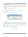
6.2. WMS Client . . . . . . . . . . . . .
6.2.1. Overview of WMS Support
6.2.2. Selecting WMS Servers . .
6.2.3. Loading WMS Layers . . .
6.2.4. Using the Identify Tool . . .
6.2.5. Viewing Properties . . . . .
6.2.6. WMS Client Limitations . .
6.3. WFS Client . . . . . . . . . . . . .
6.3.1. Loading a WFS Layer . . .
.
.
.
.
.
.
.
.
.
.
49
49
49
49
50
51
53
53
55
55
55
.
.
.
.
58
58
58
60
60
.
.
.
.
.
.
.
.
.
.
.
.
.
.
.
.
62
62
63
63
65
66
67
67
68
68
68
68
69
69
70
71
72
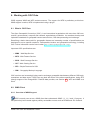
9. Making MapServer Map Files
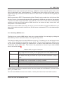
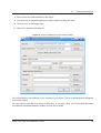
9.1. Creating the Project File . . . . . . . . . . . . . . . . . . . . . . . . . . . . . . . . . . .
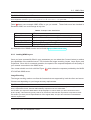
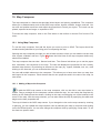
9.2. Creating the Map File . . . . . . . . . . . . . . . . . . . . . . . . . . . . . . . . . . . .
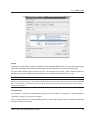
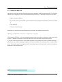
9.3. Testing the Map File . . . . . . . . . . . . . . . . . . . . . . . . . . . . . . . . . . . . .
74
74
74
77
7. Working with Projections
7.1. Overview of Projection Support
7.2. Getting Started . . . . . . . . .
7.2.1. Specifying a Projection
7.3. Custom Projections . . . . . .
.
.
.
.
.
.
.
.
.
.
.
.
.
.
.
.
.
.
.
.
.
.
.
.
.
.
.
.
.
.
.
.
.
.
.
.
.
.
.
.
.
.
.
.
.
.
.
.
.
.
8. GRASS Integration
8.1. Starting QGIS with GRASS . . . . . . .
8.2. Loading GRASS Data . . . . . . . . . .
8.3. Creating a Location . . . . . . . . . . .
8.4. Vector Data Model . . . . . . . . . . . .
8.5. Digitizing and Editing Tools . . . . . . .
8.5.1. Toolbar . . . . . . . . . . . . . .
8.5.2. Category Tab . . . . . . . . . . .
8.5.3. Settings Tab . . . . . . . . . . .
8.5.4. Symbology Tab . . . . . . . . . .
8.5.5. Table Tab . . . . . . . . . . . . .
8.6. Region Tool . . . . . . . . . . . . . . . .
8.7. GRASS Toolbox . . . . . . . . . . . . .
8.7.1. Modules inside the toolbox . . .
8.7.2. GRASS Browser . . . . . . . . .
8.7.3. Customizing the modules section
8.8. Creating a new GRASS layer . . . . . .
QGIS 0.9.0 User and Installation Guide
.
.
.
.
.
.
.
.
.
.
.
.
.
.
.
.
.
.
.
.
.
.
.
.
.
.
.
.
.
.
.
.
.
.
.
.
.
.
.
.
.
.
.
.
.
.
.
.
.
.
.
.
.
.
.
.
.
.
.
.
.
.
.
.
.
.
.
.
.
.
.
.
.
.
.
.
.
.
.
.
.
.
.
.
.
.
.
.
.
.
.
.
.
.
.
.
.
.
.
.
.
.
.
.
.
.
.
.
.
.
.
.
.
.
.
.
.
.
.
.
.
.
.
.
.
.
.
.
.
.
.
.
.
.
.
.
.
.
.
.
.
.
.
.
.
.
.
.
.
.
.
.
.
.
.
.
.
.
.
.
.
.
.
.
.
.
.
.
.
.
.
.
.
.
.
.
.
.
.
.
.
.
.
.
.
.
.
.
.
.
.
.
.
.
.
.
.
.
.
.
.
.
.
.
.
.
.
.
.
.
.
.
.
.
.
.
.
.
.
.
.
.
.
.
.
.
.
.
.
.
.
.
.
.
.
.
.
.
.
.
.
.
.
.
.
.
.
.
.
.
.
.
.
.
.
.
.
.
.
.
.
.
.
.
.
.
.
.
.
.
.
.
.
.
.
.
.
.
.
.
.
.
.
.
.
.
.
.
.
.
.
.
.
.
.
.
.
.
.
.
.
.
.
.
.
.
.
.
.
.
.
.
.
.
.
.
.
.
.
.
.
.
.
.
.
.
.
.
.
.
.
.
.
.
.
.
.
.
.
.
.
.
.
.
.
.
.
.
.
.
.
.
.
.
.
.
.
.
.
.
.
.
.
.
.
.
.
.
.
.
.
.
.
.
.
.
.
.
.
.
.
.
.
.
.
.
.
.
.
.
.
.
.
.
.
.
.
.
.
.
.
.
.
.
.
.
.
.
.
.
.
.
.
.
.
.
.
.
.
.
.
.
.
.
.
.
.
.
.
.
.
.
.
.
.
.
.
.
.
.
.
.
.
.
.
.
.
.
.
.
.
.
.
.
.
.
.
.
.
.
.
.
.
.
.
.
.
.
.
.
.
.
.
.
.
.
.
.
.
.
.
.
.
.
.
.
.
.
.
.
.
.
.
.
.
.
.
.
.
.
.
.
.
.
.
.
.
.
.
.
.
.
.
.
.
.
.
.
.
.
.
.
.
.
.
.
.
.
.
.
.
.
.
.
.
.
.
.
.
.
.
.
.
.
.
.
.
.
.
.
.
.
.
.
.
.
.
.
.
.
.
.
.
.
.
.
.
.
.
.
.
.
.
.
.
.
.
.
.
.
.
.
.
.
.
.
.
.
.
.
.
.
.
.
.
.
.
.
.
.
.
.
.
.
.
.
.
.
.
.
.
.
.
.
.
.
.
.
.
.
.
.
.
.
.
.
.
.
.
.
.
.
.
.
.
.
.
.
.
.
.
.
.
.
.
.
.
.
.
.
.
.
.
.
.
.
.
.
.
.
.
.
.
.
.
.
.
.
.
.
.
.
.
.
.
.
.
.
.
.
.
.
.
.
.
.
.
.
.
.
.
.
.
.
.
.
.
.
.
.
.
.
.
.
.
.
.
.
.
.
.
.
.
.
.
.
.
.
.
.
.
.
.
.
.
.
.
.
.
.
.
.
.
.
.
.
.
.
.
.
.
.
.
.
.
.
.
.
.
.
v
Contents
10. Map Composer
10.1.Using Map Composer . . . . . . . . . . . . . .
10.1.1. Adding a Map to the Composer . . . . .
10.1.2. Adding other Elements to the Composer
10.1.3. Other Features . . . . . . . . . . . . . .
10.1.4. Creating Output . . . . . . . . . . . . .
.
.
.
.
.
.
.
.
.
.
.
.
.
.
.
.
.
.
.
.
.
.
.
.
.
.
.
.
.
.
.
.
.
.
.
.
.
.
.
.
.
.
.
.
.
.
.
.
.
.
.
.
.
.
.
.
.
.
.
.
.
.
.
.
.
.
.
.
.
.
.
.
.
.
.
.
.
.
.
.
.
.
.
.
.
.
.
.
.
.
.
.
.
.
.
.
.
.
.
.
.
.
.
.
.
.
.
.
.
.
78
78
78
80
80
80
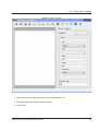
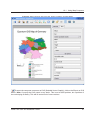
11. Using Plugins
11.1.An Introduction to Using Plugins . . . . . . .
11.1.1. Finding and Installing a Plugin . . . .
11.1.2. Managing Plugins . . . . . . . . . . .
11.1.3. Data Providers . . . . . . . . . . . . .
11.1.4. Core Plugins . . . . . . . . . . . . . .
11.1.5. External Plugins . . . . . . . . . . . .
11.1.6. Plugin templates . . . . . . . . . . . .
11.2.Using the Decorations Plugins . . . . . . . .
11.2.1. Copyright Label Plugin . . . . . . . . .
11.2.2. North Arrow Plugin . . . . . . . . . . .
11.2.3. Scale Bar Plugin . . . . . . . . . . . .
11.3.Using the GPS Plugin . . . . . . . . . . . . .
11.3.1. What is GPS? . . . . . . . . . . . . .
11.3.2. Loading GPS data from a file . . . . .
11.3.3. GPSBabel . . . . . . . . . . . . . . . .
11.3.4. Importing GPS data . . . . . . . . . .
11.3.5. Downloading GPS data from a device
11.3.6. Uploading GPS data to a device . . .
11.3.7. Defining new device types . . . . . . .
11.4.Using the Delimited Text Plugin . . . . . . . .
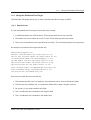
11.4.1. Requirements . . . . . . . . . . . . . .
11.4.2. Using the Plugin . . . . . . . . . . . .
11.5.Using the Graticule Creator Plugin . . . . . .
11.6.Using the Georeferencer Plugin . . . . . . . .
11.7.Using the Python Plugin . . . . . . . . . . . .
11.7.1. Setting up the Structure . . . . . . . .
11.7.2. Making the Plugin Recognizable . . .
11.7.3. Resources . . . . . . . . . . . . . . .
11.7.4. Creating the GUI . . . . . . . . . . . .
11.7.5. Creating the Plugin . . . . . . . . . . .
11.7.6. Issues and Problems . . . . . . . . . .
11.7.7. Adding Feedback . . . . . . . . . . . .
11.7.8. Summary . . . . . . . . . . . . . . . .
.
.
.
.
.
.
.
.
.
.
.
.
.
.
.
.
.
.
.
.
.
.
.
.
.
.
.
.
.
.
.
.
.
.
.
.
.
.
.
.
.
.
.
.
.
.
.
.
.
.
.
.
.
.
.
.
.
.
.
.
.
.
.
.
.
.
.
.
.
.
.
.
.
.
.
.
.
.
.
.
.
.
.
.
.
.
.
.
.
.
.
.
.
.
.
.
.
.
.
.
.
.
.
.
.
.
.
.
.
.
.
.
.
.
.
.
.
.
.
.
.
.
.
.
.
.
.
.
.
.
.
.
.
.
.
.
.
.
.
.
.
.
.
.
.
.
.
.
.
.
.
.
.
.
.
.
.
.
.
.
.
.
.
.
.
.
.
.
.
.
.
.
.
.
.
.
.
.
.
.
.
.
.
.
.
.
.
.
.
.
.
.
.
.
.
.
.
.
.
.
.
.
.
.
.
.
.
.
.
.
.
.
.
.
.
.
.
.
.
.
.
.
.
.
.
.
.
.
.
.
.
.
.
.
.
.
.
.
.
.
.
.
.
.
.
.
.
.
.
.
.
.
.
.
.
.
.
.
.
.
.
.
.
.
.
.
.
.
.
.
.
.
.
.
.
.
.
.
.
.
.
.
.
.
.
.
.
.
.
.
.
.
.
.
.
.
.
.
.
.
.
.
.
.
.
.
.
.
.
.
.
.
.
.
.
.
.
.
.
.
.
.
.
.
.
.
.
.
.
.
.
.
.
.
.
.
.
.
.
.
.
.
.
.
.
.
.
.
.
.
.
.
.
.
.
.
.
.
.
.
.
.
.
.
.
.
.
.
.
.
.
.
.
.
.
.
.
.
.
.
.
.
.
.
.
.
.
.
.
.
.
.
.
.
.
.
.
.
.
.
.
.
.
.
.
.
.
.
.
.
.
.
.
.
.
.
.
.
.
.
.
.
.
.
.
.
.
.
.
.
.
.
.
.
.
.
.
.
.
.
.
.
.
.
.
.
.
.
.
.
.
.
.
.
.
.
.
.
.
.
.
.
.
.
.
.
.
.
.
.
.
.
.
.
.
.
.
.
.
.
.
.
.
.
.
.
.
.
.
.
.
.
.
.
.
.
.
.
.
.
.
.
.
.
.
.
.
.
.
.
.
.
.
.
.
.
.
.
.
.
.
.
.
.
.
.
.
.
.
.
.
.
.
.
.
.
.
.
.
.
.
.
.
.
.
.
.
.
.
.
.
.
.
.
.
.
.
.
.
.
.
.
.
.
.
.
.
.
.
.
.
.
.
.
.
.
.
.
.
.
.
.
.
.
.
.
.
.
.
.
.
.
.
.
.
.
.
.
.
.
.
.
.
.
.
.
.
.
.
.
.
.
.
.
.
.
.
.
.
.
.
.
.
.
.
.
.
.
.
.
.
.
.
.
.
.
.
.
.
.
.
.
.
.
.
.
.
.
.
.
.
.
.
.
.
.
.
.
.
.
.
.
.
.
.
.
.
.
.
.
.
.
.
.
.
.
.
.
.
.
.
.
.
.
.
.
.
.
.
.
.
.
.
.
.
.
.
.
.
.
.
.
.
.
.
.
.
.
.
.
.
.
.
.
.
.
.
.
.
.
.
.
.
.
.
.
82
82
82
82
83
83
84
85
86
86
87
87
89
89
89
90
90
90
91
91
93
93
94
96
97
101
101
102
102
103
103
107
108
108
QGIS 0.9.0 User and Installation Guide
.
.
.
.
.
.
.
.
.
.
.
.
.
.
.
.
.
.
.
.
.
.
.
.
.
.
.
.
.
.
.
.
.
vi
Contents
12. Creating Applications
12.1.Designing the GUI . . . .
12.2.Creating the MainWindow
12.3.Finishing Up . . . . . . .
12.4.Running the Application .
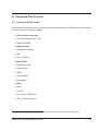
13. Help and Support
13.1.Mailinglists .
13.2.IRC . . . . .
13.3.BugTracker .
13.4.Blog . . . . .
13.5.Wiki . . . . .
.
.
.
.
.
.
.
.
.
.
.
.
.
.
.
.
.
.
.
.
.
.
.
.
.
.
.
.
.
.
.
.
.
.
.
.
.
.
.
.
.
.
.
.
.
.
.
.
.
.
.
.
.
.
.
.
.
.
.
.
.
.
.
.
.
.
.
.
.
.
.
.
.
.
.
.
.
.
.
.
.
.
.
.
.
.
.
.
.
.
.
.
.
.
.
.
.
.
.
.
.
.
.
.
.
.
.
.
.
.
.
.
.
.
.
.
.
.
.
.
.
.
.
.
.
.
.
.
.
.
.
.
.
.
.
.
.
.
.
.
.
.
.
.
.
.
.
.
.
.
.
.
.
.
.
.
.
.
.
.
.
.
.
.
.
.
.
.
.
.
.
.
.
.
.
.
.
.
.
.
.
.
.
.
.
.
.
.
.
.
.
.
.
.
.
.
.
.
.
.
.
.
.
.
.
.
.
.
.
.
.
.
.
.
.
.
.
.
.
.
.
.
.
.
.
.
.
.
.
.
.
.
.
.
.
.
.
.
.
.
.
.
.
.
.
.
.
.
.
.
.
.
.
.
.
.
.
.
.
.
.
.
.
.
.
.
.
.
.
.
.
.
.
.
.
.
.
.
.
.
.
.
.
.
.
.
.
.
.
.
.
.
.
.
.
.
.
.
.
.
.
.
.
.
.
.
.
.
.
.
.
.
.
.
.
.
.
.
.
.
.
.
.
.
.
.
.
.
.
.
.
.
.
.
.
.
109
109
110
115
115
.
.
.
.
.
118
118
119
119
119
120
A. Supported Data Formats
121
A.1. Supported OGR Formats . . . . . . . . . . . . . . . . . . . . . . . . . . . . . . . . . . 121
A.2. GDAL Raster Formats . . . . . . . . . . . . . . . . . . . . . . . . . . . . . . . . . . . . 122
B. Building under windows using msys
B.1. MSYS: . . . . . . . . . . . . . . . . . . . . . . . . . . . . . . . . . . . . . . . . . .
B.2. Qt4.3 . . . . . . . . . . . . . . . . . . . . . . . . . . . . . . . . . . . . . . . . . .
B.3. Flex and Bison . . . . . . . . . . . . . . . . . . . . . . . . . . . . . . . . . . . . .
B.4. Python stuff: (optional) . . . . . . . . . . . . . . . . . . . . . . . . . . . . . . . . .
B.4.1. Download and install Python - use Windows installer . . . . . . . . . . . .
B.4.2. Download SIP and PyQt4 sources . . . . . . . . . . . . . . . . . . . . . .
B.4.3. Compile SIP . . . . . . . . . . . . . . . . . . . . . . . . . . . . . . . . . .
B.4.4. Compile PyQt . . . . . . . . . . . . . . . . . . . . . . . . . . . . . . . . . .
B.4.5. Final python notes . . . . . . . . . . . . . . . . . . . . . . . . . . . . . . .
B.5. Subversion: . . . . . . . . . . . . . . . . . . . . . . . . . . . . . . . . . . . . . . .
B.6. CMake: . . . . . . . . . . . . . . . . . . . . . . . . . . . . . . . . . . . . . . . . .
B.7. QGIS: . . . . . . . . . . . . . . . . . . . . . . . . . . . . . . . . . . . . . . . . . .
B.8. Compiling: . . . . . . . . . . . . . . . . . . . . . . . . . . . . . . . . . . . . . . . .
B.9. Configuration . . . . . . . . . . . . . . . . . . . . . . . . . . . . . . . . . . . . . .
B.10.Compilation and installation . . . . . . . . . . . . . . . . . . . . . . . . . . . . . .
B.11.Run qgis.exe from the directory where it’s installed (CMAKE_INSTALL_PREFIX)
B.12.Create the installation package: (optional) . . . . . . . . . . . . . . . . . . . . . .
.
.
.
.
.
.
.
.
.
.
.
.
.
.
.
.
.
.
.
.
.
.
.
.
.
.
.
.
.
.
.
.
.
.
.
.
.
.
.
.
.
.
.
.
.
.
.
.
.
.
.
124
124
124
125
125
125
125
125
126
126
126
126
126
127
127
128
128
128
C. Building on Mac OSX using frameworks and cmake (QGIS > 0.8)
C.1. Install XCODE . . . . . . . . . . . . . . . . . . . . . . . . . . . .
C.2. Install Qt4 from .dmg . . . . . . . . . . . . . . . . . . . . . . . . .
C.3. Install development frameworks for QGIS dependencies . . . . .
C.3.1. Additional Dependencies : GSL . . . . . . . . . . . . . . .
C.3.2. Additional Dependencies : Expat . . . . . . . . . . . . . .
C.3.3. Additional Dependencies : SIP . . . . . . . . . . . . . . .
.
.
.
.
.
.
.
.
.
.
.
.
.
.
.
.
.
.
128
128
129
129
130
130
130
QGIS 0.9.0 User and Installation Guide
.
.
.
.
.
.
.
.
.
.
.
.
.
.
.
.
.
.
.
.
.
.
.
.
.
.
.
.
.
.
.
.
.
.
.
.
.
.
.
.
.
.
.
.
.
.
.
.
.
.
.
.
.
.
vii
Contents
C.4.
C.5.
C.6.
C.7.
C.8.
C.9.
C.3.4. Additional Dependencies :
C.3.5. Additional Dependencies :
Install CMAKE for OSX . . . . .
Install subversion for OSX . . . .
Check out QGIS from SVN . . .
Configure the build . . . . . . . .
GEOS Issues . . . . . . . . . . .
Building . . . . . . . . . . . . . .
PyQt
Bison
. . . .
. . . .
. . . .
. . . .
. . . .
. . . .
.
.
.
.
.
.
.
.
.
.
.
.
.
.
.
.
.
.
.
.
.
.
.
.
.
.
.
.
.
.
.
.
.
.
.
.
.
.
.
.
.
.
.
.
.
.
.
.
.
.
.
.
.
.
.
.
.
.
.
.
.
.
.
.
.
.
.
.
.
.
.
.
.
.
.
.
.
.
.
.
.
.
.
.
.
.
.
.
D. Building on GNU/Linux
D.1. Building QGIS with Qt4.x . . . . . . . . . . . . . . . . . . .
D.2. Prepare apt . . . . . . . . . . . . . . . . . . . . . . . . . . .
D.3. Install Qt4 . . . . . . . . . . . . . . . . . . . . . . . . . . . .
D.4. Install additional software dependencies required by QGIS .
D.5. GRASS Specific Steps . . . . . . . . . . . . . . . . . . . . .
D.6. Setup ccache (Optional) . . . . . . . . . . . . . . . . . . . .
D.7. Prepare your development environment . . . . . . . . . . .
D.8. Check out the QGIS Source Code . . . . . . . . . . . . . .
D.9. Starting the compile . . . . . . . . . . . . . . . . . . . . . .
D.10.Running QGIS . . . . . . . . . . . . . . . . . . . . . . . . .
.
.
.
.
.
.
.
.
.
.
.
.
.
.
.
.
.
.
.
.
.
.
.
.
.
.
.
.
.
.
.
.
.
.
.
.
E. Creation of MSYS environment for compilation of Quantum GIS
E.1. Initial setup . . . . . . . . . . . . . . . . . . . . . . . . . . . . .
E.1.1. MSYS . . . . . . . . . . . . . . . . . . . . . . . . . . . .
E.1.2. MinGW . . . . . . . . . . . . . . . . . . . . . . . . . . .
E.1.3. Flex and Bison . . . . . . . . . . . . . . . . . . . . . . .
E.2. Installing dependencies . . . . . . . . . . . . . . . . . . . . . .
E.2.1. Getting ready . . . . . . . . . . . . . . . . . . . . . . . .
E.2.2. GDAL level one . . . . . . . . . . . . . . . . . . . . . . .
E.2.3. GRASS . . . . . . . . . . . . . . . . . . . . . . . . . . .
E.2.4. GDAL level two . . . . . . . . . . . . . . . . . . . . . . .
E.2.5. GEOS . . . . . . . . . . . . . . . . . . . . . . . . . . . .
E.2.6. SQLITE . . . . . . . . . . . . . . . . . . . . . . . . . . .
E.2.7. GSL . . . . . . . . . . . . . . . . . . . . . . . . . . . . .
E.2.8. EXPAT . . . . . . . . . . . . . . . . . . . . . . . . . . . .
E.2.9. POSTGRES . . . . . . . . . . . . . . . . . . . . . . . .
E.3. Cleanup . . . . . . . . . . . . . . . . . . . . . . . . . . . . . . .
F. GNU General Public License
F.1. Quantum GIS Qt exception for GPL
Cited literature
QGIS 0.9.0 User and Installation Guide
.
.
.
.
.
.
.
.
.
.
.
.
.
.
.
.
.
.
.
.
.
.
.
.
.
.
.
.
.
.
.
.
.
.
.
.
.
.
.
.
.
.
.
.
.
.
.
.
.
.
.
.
.
.
.
.
.
.
.
.
.
.
.
.
.
.
.
.
.
.
.
.
.
.
.
.
.
.
.
.
.
.
.
.
.
.
.
.
.
.
.
.
.
.
.
.
.
.
.
.
.
.
.
.
.
.
.
.
.
.
.
.
.
.
.
.
.
.
.
.
.
.
.
.
.
.
.
.
.
.
.
.
.
.
.
.
.
.
.
.
.
.
.
.
.
.
.
.
.
.
.
.
.
.
.
.
.
.
.
.
.
.
.
.
.
.
.
.
.
.
.
.
.
.
.
.
.
.
.
.
.
.
.
.
.
.
.
.
.
.
.
.
.
.
.
.
.
.
.
.
.
.
.
.
.
.
.
.
.
.
.
.
.
.
.
.
.
.
.
.
.
.
.
.
.
.
.
.
.
.
.
.
.
.
.
.
.
.
.
.
.
.
.
.
.
.
.
.
.
.
.
.
.
.
.
.
.
.
.
.
.
.
.
.
.
.
.
.
.
.
.
.
.
.
.
.
.
.
.
.
.
.
.
.
.
.
.
.
.
.
.
.
.
.
.
.
.
.
.
.
.
.
.
.
.
.
.
.
.
.
.
.
.
.
.
.
.
.
.
.
.
.
.
.
.
.
.
.
.
.
.
.
.
.
.
.
.
.
.
.
.
.
.
.
.
.
.
.
.
.
.
.
.
.
.
.
.
.
.
.
.
.
.
.
.
.
.
.
.
.
.
.
.
.
.
.
.
.
.
.
.
.
.
.
.
.
.
.
.
.
.
.
.
.
.
.
.
.
.
.
.
.
.
.
131
131
132
132
133
134
134
134
.
.
.
.
.
.
.
.
.
.
135
135
135
135
136
136
137
137
137
138
139
.
.
.
.
.
.
.
.
.
.
.
.
.
.
.
139
139
139
139
140
140
140
141
143
143
144
145
145
145
146
146
147
. . . . . . . . . . . . . . . . . . . . . . . . . . . . 152
153
viii
Contents
Index
QGIS 0.9.0 User and Installation Guide
154
ix
List of Figures
List of Figures
1.
2.
3.
4.
5.
6.
7.
8.
9.
10.
11.
12.
13.
14.
15.
16.
17.
18.
19.
20.
21.
22.
23.
24.
25.
26.
27.
28.
29.
30.
31.
32.
33.
34.
35.
36.
37.
38.
39.
40.
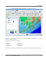
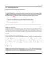
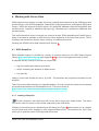
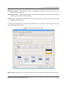
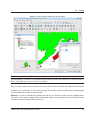
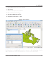
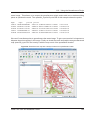
Main window with alaska sample data (GNU/Linux with KDE) . . . .
Measure tools in action . . . . . . . . . . . . . . . . . . . . . . . . .
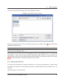
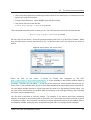
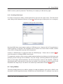
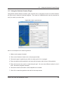
Open OGR Data Source Dialog . . . . . . . . . . . . . . . . . . . . .
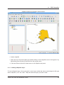
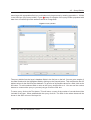
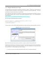
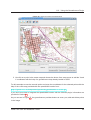
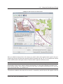
QGIS with Shapefile of Alaska loaded . . . . . . . . . . . . . . . . .
Vector Layer Properties Dialog . . . . . . . . . . . . . . . . . . . . .
Select feature and choose action . . . . . . . . . . . . . . . . . . . .
Vector Digitizing Attributes Capture Dialog . . . . . . . . . . . . . . .
Creating a New Vector Dialog . . . . . . . . . . . . . . . . . . . . . .
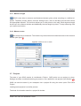
Query Builder . . . . . . . . . . . . . . . . . . . . . . . . . . . . . . .
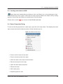
Raster context menu . . . . . . . . . . . . . . . . . . . . . . . . . . .
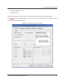
Raster Layers Properties Dialog . . . . . . . . . . . . . . . . . . . .
Dialog for adding a WMS server, showing its available layers . . . .
Adding a WFS layer . . . . . . . . . . . . . . . . . . . . . . . . . . .
Projection Dialog (GNU/Linux) . . . . . . . . . . . . . . . . . . . . .
Custom Projection Dialog (OS X) . . . . . . . . . . . . . . . . . . . .
Creating a GRASS location in QGIS . . . . . . . . . . . . . . . . . .
GRASS Edit Dialog . . . . . . . . . . . . . . . . . . . . . . . . . . . .
GRASS toolbox . . . . . . . . . . . . . . . . . . . . . . . . . . . . . .
Module generated through parsing the XML-file . . . . . . . . . . . .
Export to MapServer map module in QGIS . . . . . . . . . . . . . .
Map Composer . . . . . . . . . . . . . . . . . . . . . . . . . . . . . .
Map Composer with map view, legend, scalebar, and text added . .
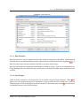
Plugin Manager . . . . . . . . . . . . . . . . . . . . . . . . . . . . . .
Copyright Plugin . . . . . . . . . . . . . . . . . . . . . . . . . . . . .
North Arrow Plugin . . . . . . . . . . . . . . . . . . . . . . . . . . . .
Scale Bar Plugin . . . . . . . . . . . . . . . . . . . . . . . . . . . . .
The GPS Tools dialog window . . . . . . . . . . . . . . . . . . . . . .
File selection dialog for the import tool . . . . . . . . . . . . . . . . .
The download tool . . . . . . . . . . . . . . . . . . . . . . . . . . . .
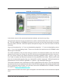
Delimited Text Dialog . . . . . . . . . . . . . . . . . . . . . . . . . . .
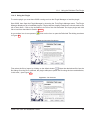
File Selected . . . . . . . . . . . . . . . . . . . . . . . . . . . . . . .
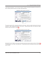
Fields Parsed from Text File . . . . . . . . . . . . . . . . . . . . . . .
Selecting the X and Y Fields . . . . . . . . . . . . . . . . . . . . . .
Create a graticule layer . . . . . . . . . . . . . . . . . . . . . . . . .
Select an image to georeference . . . . . . . . . . . . . . . . . . . .
Select an image to georeference . . . . . . . . . . . . . . . . . . . .
Add points to the raster image . . . . . . . . . . . . . . . . . . . . .
Georeferenced map with overlayed roads from spearfish60 location
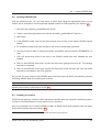
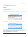
Enter new PostGIS table name . . . . . . . . . . . . . . . . . . . . .
Enter field names for new PostGIS table . . . . . . . . . . . . . . . .
QGIS 0.9.0 User and Installation Guide
.
.
.
.
.
.
.
.
.
.
.
.
.
.
.
.
.
.
.
.
.
.
.
.
.
.
.
.
.
.
.
.
.
.
.
.
.
.
.
.
.
.
.
.
.
.
.
.
.
.
.
.
.
.
.
.
.
.
.
.
.
.
.
.
.
.
.
.
.
.
.
.
.
.
.
.
.
.
.
.
.
.
.
.
.
.
.
.
.
.
.
.
.
.
.
.
.
.
.
.
.
.
.
.
.
.
.
.
.
.
.
.
.
.
.
.
.
.
.
.
.
.
.
.
.
.
.
.
.
.
.
.
.
.
.
.
.
.
.
.
.
.
.
.
.
.
.
.
.
.
.
.
.
.
.
.
.
.
.
.
.
.
.
.
.
.
.
.
.
.
.
.
.
.
.
.
.
.
.
.
.
.
.
.
.
.
.
.
.
.
.
.
.
.
.
.
.
.
.
.
.
.
.
.
.
.
.
.
.
.
.
.
.
.
.
.
.
.
.
.
.
.
.
.
.
.
.
.
.
.
.
.
.
.
.
.
.
.
.
.
.
.
.
.
.
.
.
.
.
.
.
.
.
.
.
.
.
.
.
.
.
.
.
.
.
.
.
.
.
.
.
.
.
.
.
.
.
.
.
.
.
.
.
.
.
.
.
.
.
.
.
.
.
.
.
.
.
.
.
.
.
.
.
.
.
.
.
.
.
.
.
.
.
.
.
.
.
.
.
.
.
.
.
.
.
.
.
.
.
.
.
.
.
.
.
.
.
.
.
.
.
.
.
.
.
.
.
.
.
.
.
.
.
.
.
.
.
.
.
.
. 10
. 17
. 21
. 22
. 28
. 33
. 37
. 40
. 41
. 44
. 45
. 52
. 56
. 59
. 60
. 64
. 66
. 71
. 72
. 76
. 79
. 81
. 83
. 86
. 87
. 88
. 89
. 91
. 92
. 94
. 94
. 95
. 95
. 96
. 97
. 98
. 99
. 100
. 106
. 106
x
List of Figures
41.
42.
43.
44.
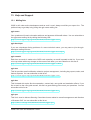
Enter DSN for connection to PostGIS database
Message Box with Plugin results . . . . . . . .
Starting the new demo application . . . . . . .
Adding a layer the demo application . . . . . .
QGIS 0.9.0 User and Installation Guide
.
.
.
.
.
.
.
.
.
.
.
.
.
.
.
.
.
.
.
.
.
.
.
.
.
.
.
.
.
.
.
.
.
.
.
.
.
.
.
.
.
.
.
.
.
.
.
.
.
.
.
.
.
.
.
.
.
.
.
.
.
.
.
.
.
.
.
.
.
.
.
.
.
.
.
.
.
.
.
.
.
.
.
.
.
.
.
.
107
108
116
116
xi
List of Tables
List of Tables
1.
2.
3.
4.
5.
PostGIS Connection Parameters
WMS Connection Parameters . .
Example Public WMS URLs . . .
GRASS Digitizing Tools . . . . .
QGIS Core Plugins . . . . . . . .
QGIS 0.9.0 User and Installation Guide
.
.
.
.
.
.
.
.
.
.
.
.
.
.
.
.
.
.
.
.
.
.
.
.
.
.
.
.
.
.
.
.
.
.
.
.
.
.
.
.
.
.
.
.
.
.
.
.
.
.
.
.
.
.
.
.
.
.
.
.
.
.
.
.
.
.
.
.
.
.
.
.
.
.
.
.
.
.
.
.
.
.
.
.
.
.
.
.
.
.
.
.
.
.
.
.
.
.
.
.
.
.
.
.
.
.
.
.
.
.
.
.
.
.
.
.
.
.
.
.
.
.
.
.
.
.
.
.
.
.
.
.
.
.
.
.
.
.
.
.
.
.
.
.
.
.
.
.
.
.
24
50
51
67
84
xii
1. Forward
Welcome to the wonderful world of Geographical Information Systems (GIS)! Quantum GIS (QGIS)
is an Open Source Geographic Information System. The project was born in May of 2002 and was
established as a project on SourceForge in June of the same year. We’ve worked hard to make
GIS software (which is traditionaly expensive commerical software) a viable prospect for anyone with
basic access to a Personal Computer. QGIS currently runs on most Unix platforms, Windows, and
OS X. QGIS is developed using the Qt toolkit (http://www.trolltech.com) and C++. This means
that QGIS feels snappy to use and has a pleasing, easy to use graphical user interface.
QGIS aims to be an easy to use GIS, providing common functions and features. The initial goal
was to provide a GIS data viewer. QGIS has reached that point in its evolution and is being used
by many for their daily GIS data viewing needs. QGIS supports a number of raster and vector data
formats, with new support easily added using the plugin architecture (see Appendix A for a full list of
currenly supported data formats). QGIS is released under the GNU General Public License (GPL).
Developing QGIS under this license means that you can inspect and modify the source code and
guarantees that you, our happy user will always have access to a GIS program that is free of cost and
can be freely modified. You should have received a full copy of the license with your copy of QGIS,
and you also find it as Appendix F.
Note: The latest version of this document can always be found at
http://qgis.org/docs/userguide.pdf
1.1. Features
QGIS has many common GIS features and functions. The major features are listed below, devided
into Core Features and Plugins.
Core Features
• Raster and vector support by the OGR library
• Support for spatially enabled PostgreSQL tables using PostGIS
• GRASS integration, including view, edit, and analysis
• Digitizing GRASS and OGR/Shapefile
• Map Composer
• OGC support
QGIS 0.9.0 User and Installation Guide
1
1.1 Features
• Overview panel
• Spatial bookmarks
• Identify/Select features
• Edit/View/Search attributes
• Feature labeling
• On the fly projection
• Save and restore projects
• Export to Mapserver map file
• Change vector and raster symbology
• Extensible plugin architecture
Plugins
• Add WFS Layer
• Add Delimited Text Layer
• Decorations (Copyright Label, North Arrow and Scale bar)
• Georeferencer
• GPS Tools
• GRASS
• Graticule Creator
• PostgreSQL Geoprocessing functions
• SPIT Shapefile to PostgreSQL/PostGIS Import Tool
• Python Console
• openModeller
QGIS 0.9.0 User and Installation Guide
2
1.2 Whats New in 0.9.0
1.2. Whats New in 0.9.0
As usual the new version 0.9.0 bring some very interesting features to you.
• Python language bindings to write plugins in Python and to create GIS enabled applications in
Python that use the QGIS libraries
• Removed automake build system - QGIS now needs CMake for compilation
• Many new GRASS modules added to the GRASS toolbox
• Map Composer updates
• Fix for 2.5D shapefiles
• Improvements to the Georeferencer
• Localization support extended to 26 languages
QGIS 0.9.0 User and Installation Guide
3
2. Introduction To GIS
A Geographical Information System (GIS)(1)1 is a collection of software that allows you to create,
visualise, query and analyse geospatial data. Geospatial data refers to information about the geographic location of an entity. This often involves the use of a geographic coordinate, like a latitude
or longitude value. Spatial data is another commonly used term, as are: geographic data, GIS data,
map data, location data, coordinate data and spatial geometry data.
Applications using geospatial data perform a variety of functions. Map production is the most easily
understood function of geospatial applications. Mapping programs take geospatial data and render
it in a form that is viewable, usually on a computer screen or printed page. Applications can present
static maps (a simple image) or dynamic maps that are customised by the person viewing the map
through a desktop program or a web page.
Many people mistakenly assume that geospatial applications just produce maps, but geospatial data
analysis is another primary function of geospatial applications. Some typical types of analysis include
computing:
1. distances between geographic locations
2. the amount of area (e.g., square metres) within a certain geographic region
3. what geographic features overlap other features
4. the amount of overlap between features
5. the number of locations within a certain distance of another
6. and so on...
These may seem simplistic, but can be applied in all sorts of ways across many disciplines. The results of analysis may be shown on a map, but are often tabulated into a report to support management
decisions.
The recent phenomena of location-based services promises to introduce all sorts of other features,
but many will be based on a combination of maps and analysis. For example, you have a cell phone
that tracks your geographic location. If you have the right software, your phone can tell you what kind
of restaurants are within walking distance. While this is a novel application of geospatial technology,
it is essentially doing geospatial data analysis and listing the results for you.
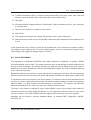
1
This chapter is by Tyler Mitchell (http://www.oreillynet.com/pub/wlg/7053) and used under the Creative Commons License. Tyler is the author of Web Mapping Illustrated, published by O’Reilly, 2005.
QGIS 0.9.0 User and Installation Guide
4
2.1 Why is all this so new?
2.1. Why is all this so new?
Well, it’s not. There are many new hardware devices that are enabling mobile geospatial services.
Many open source geospatial applications are also available, but the existence of geospatially focused hardware and software is nothing new. Global positioning system (GPS) receivers are becoming commonplace, but have been used in various industries for more than a decade. Likewise,
desktop mapping and analysis tools have also been a major commercial market, primarily focused
on industries such as natural resource management.
What is new, is how the latest hardware and software is being applied and who is applying it. Traditional users of mapping and analysis tools were highly trained GIS Analysts or digital mapping
technicians trained to use CAD-like tools. Now, the processing capabilities of home PC’s and open
source software packages have enabled an army of hobbyists, professionals, web developers, etc. to
interact with geospatial data. The learning curve has come down. The costs have come down. The
amount of geospatial technology saturation has increased.
How is geospatial data stored? In a nutshell, there are two types of geospatial data in widespread
use today. This is in additional to traditional tabular data that is also widely used by geospatial
applications.
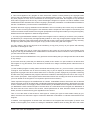
2.1.1. Raster Data
One type of geospatial data is called raster data or simply "a raster". The most easily recognised form
of raster data is digital satellite imagery or air photos. Elevation shading or digital elevation models
are also typically represented as raster data. Any type of map feature can be represented as raster
data, but there are limitations.
A raster is a regular grid made up of cells, or in the case of imagery, pixels. They have a fixed number
of rows and columns. Each cell has a numeric value and has a certain geographic size (e.g. 30x30
meters in size).
Multiple overlapping rasters are used to represent images using more than one colour value (i.e. one
raster for each set of red, green and blue values is combined to create a colour image). Satellite
imagery also represents data in multiple "bands". Each band is essentially a separate, spatially
overlapping raster where each band holds values of certain wavelengths of light. As you can imagine,
a large raster takes up more file space. A raster with smaller cells can provide more detail, but takes
up more file space. The trick is finding the right balance between cell size for storage purposes and
cell size for analytical or mapping purposes.
QGIS 0.9.0 User and Installation Guide
5
2.1 Why is all this so new?
2.1.2. Vector Data
Vector data is also used in geospatial applications. If you stayed awake during trigonometry and
coordinate geometry classes, you will already be familiar with some of the qualities of vector data.
In its simplest sense, vectors are a way of describing a location by using a set of coordinates. Each
coordinate refers to a geographic location using a system of x and y values.
This can be thought of in reference to a Cartesian plane - you know, the diagrams from school
that showed an x and y-axis. You might have used them to chart declining retirement savings or
increasing compound mortgage interest, but the concepts are essential to geospatial data analysis
and mapping.
There are various ways of representing these geographic coordinates depending on your purpose.
This is a whole area of study for another day - map projections.
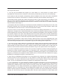
Vector data takes on three forms, each progressively more complex and building on the former.
1. Points - A single coordinate (x y) represents the discrete geographic location
2. Lines - Multiple coordinates (x1 y1, x2 y2, x3 y4, ... xn yn) strung together in a certain order.
Like drawing a line from Point (x1 y1) to Point (x2 y2) and so on. These parts between each
point are considered line segments. They have a length and the line can be said to have a
direction based on the order of the points. Technically, a line is a single pair of coordinates
connected together; whereas, a line string is multiple lines connected together.
3. Polygons - When lines are strung together by more than two points, with the last point being at
the same location as the first, we call this a polygon. A triangle, circle, rectangle, etc. are all
polygons. The key feature of polygons is that there is a fixed area within them.
QGIS 0.9.0 User and Installation Guide
6
3. Getting Started
This chapter gives a quick overview of running QGIS with data available on the QGIS web page.
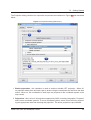
3.1. Installation
Building QGIS from source is documented in Appendix B for windows, Appendix C for Mac OSX and
Appendix D for GNU/Linux. The Installation instructions are distributed with the QGIS source code
and also available at http://qgis.org.
Standard installer packages are available for Windows and Mac OS X. For many flavors of GNU/Linux
binary packages are provided. Get the latest information on binary packages at the QGIS website at
http://download.qgis.org.
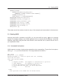
3.2. Sample Data
If you do not have any GIS data handy, you can obtain an Alaska dataset from the QGIS web site at
http://qgis.org. The projection for the data is Alaska Albers Equal Area with unit meter:
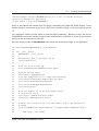
PROJCS["NAD_1927_Albers",
GEOGCS["GCS_North_American_1927",
DATUM ["D_North_American_1927",
SPHEROID["Clarke_1866", 6378206.4,294.9786982]],
PRIMEM["Greenwich",0.0],
UNIT["Degree", 0.0174532925199433]],
PROJECTION["Albers"],
PARAMETER["False_Easting", 0.0],
PARAMETER["False_Northing",0.0],
PARAMETER["Central_Meridian",-154.0],
PARAMETER["Standard_Parallel_1", 55.0],
PARAMETER["Standard_Parallel_2",65.0],
PARAMETER ["Latitude_Of_Origin",50.0],
UNIT["Meter",1.0]]
For use with GRASS, a sample GRASS database (e.g. Spearfish) can be obtained from the official
GRASS GIS-website http://grass.itc.it/download/data.php. The projection of the Spearfish
dataset is UTM Zone 13, Northern Hemisphere:
PROJCS["UTM Zone 13, Northern Hemisphere",
QGIS 0.9.0 User and Installation Guide
7
3.3 Starting QGIS
GEOGCS["clark66",
DATUM["North_American_Datum_1927",
SPHEROID["clark66",6378206.4,294.9786982]],
PRIMEM["Greenwich",0],
UNIT["degree",0.0174532925199433]],
PROJECTION["Transverse_Mercator"],
PARAMETER["latitude_of_origin",0],
PARAMETER["central_meridian",-105],
PARAMETER["scale_factor",0.9996],
PARAMETER["false_easting",500000],
PARAMETER["false_northing",0],
UNIT["meter",1]]
These data sets will be used as a basis for many of the examples and screenshots in this document.
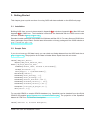
3.3. Starting QGIS
Assuming that QGIS is installed in the PATH, you can start QGIS by typing: qgis at a command
prompt or by double clicking on the QGIS application link (or shortcut) on the desktop. Under MS
Windows, start QGIS using the Start menu shortcut, and under Mac OS X, double click the icon in
your Applications folder.
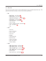
3.3.1. Command Line Options
QGIS supports a number of options when started from the command line. To get a list of the options,
enter qgis --help on the command line. The usage statement for QGIS is:
qgis --help
Quantum GIS - 0.9.0 ’Ganymede’
Quantum GIS (QGIS) is a viewer for spatial data sets, including
raster and vector data.
Usage: qgis [options] [FILES]
options:
[--snapshot filename]
emit snapshot of loaded datasets to given file
[--lang language]
use language for interface text
[--project projectfile] load the given QGIS project
[--extent xmin,ymin,xmax,ymax] set initial map extent
[--help]
this text
FILES:
Files specified on the command line can include rasters,
QGIS 0.9.0 User and Installation Guide
8
3.4 QGIS GUI
vectors, and QGIS project files (.qgs):
1. Rasters - Supported formats include GeoTiff, DEM
and others supported by GDAL
2. Vectors - Supported formats include ESRI Shapefiles
and others supported by OGR and PostgreSQL layers using
the PostGIS extension
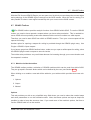
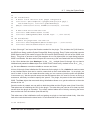
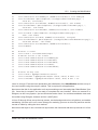
Tip 1 E XAMPLE U SING
COMMAND LINE ARGUMENTS
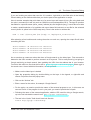
You can start QGIS by specifying one or more data files on the command line. For example, assuming you
are in your data directory, you could start QGIS with two shapefiles and a raster file set to load on startup
using the following command: qgis ak_shade.tif alaska.shp majrivers.shp
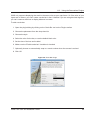
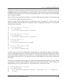
Command line option --snapshot
This option allows you to create a snapshot in PNG format from the current view. This comes in
handy when you have a lot of projects and want to generate snapshots from your data.
Currently it generates a PNG-file with 800x600 pixels. A filename can be added after --snapshot.
Command line option --lang
Based on your locale QGIS, selects the correct localization. If you like to change your language, you
can provide another language with this option.
Command line option --project
Starting QGIS with an existing project file is also possible. Just add the command line option
-project followed by your project name and QGIS will open with all layers loaded described in the
given file.
Command line option --extent
To start with a specific map extent use this option. You need to add the bounding box of your extent
in the following order separated by a comma:
--extent xmin,ymin,xmax,ymax
3.4. QGIS GUI
When QGIS starts, you are presented with the GUI as shown below (the numbers 1 through 6 in blue
ovals refer to the six major areas of the interface as discussed below):
QGIS 0.9.0 User and Installation Guide
9
3.4 QGIS GUI
Figure 1: Main window with alaska sample data (GNU/Linux with KDE)
Note: Your window decorations (title bar, etc.) may appear different depending on your operating
system and window manager.
The QGIS GUI is divided into six areas:
1. Menu Bar
2. Tool Bar
3. Map Legend
4. Map View
5. Map Overview
6. Status Bar
These six components of the QGIS interface are described in more detail in the following sections.
QGIS 0.9.0 User and Installation Guide
10
3.4 QGIS GUI
3.4.1. Menu Bar
The menu bar provides access to various QGIS features using a standard hierarchical menu. The
top-level menus and a summary of some of the functions provided are:
• File
– New Project - see Section 3.7
– Open Project - see Section 3.7
– Open Recent Projects - see Section 3.7
– Save Project - see Section 3.7
– Save Project As - see Section 3.7
– Save as Image
– Export to MapServer Map - see Section 9
– Print - see Section 10
– Exit
• View
– Zoom Full
– Zoom To Selection
– Zoom To Layer
– Zoom Last
– Refresh
– Show Bookmarks
– New Bookmark
– Show most toolbars
– Hide most toolbars
– Toolbar Visibility
• Layer
– Add a Vector Layer - see Section 4
– Add a Raster Layer - see Section 5
– Add a PostGIS Layer - see Section 4.2
– Add a WMS Layer - see Section 6.2
– Remove Layer
– New Vector Layer - see Section 4.4.3
QGIS 0.9.0 User and Installation Guide
11
3.4 QGIS GUI
– In Overview
– Add All To Overview
– Remove All From Overview
– Hide All Layers
– Show All Layers
• Settings
– Project Properties - see Section 3.7
– Custom Projection - see Section 7.3
– Options - see Section 3.8
• Plugins - (Futher menu items are added by plugins as they are loaded.)
– Plugin Manager - see Section 11.1.2
• Help
– Help Contents
– QGIS Homepage
– Check QGIS Version
– About
3.4.2. Toolbars
The toolbars provide access to most of the same functions as the menus, plus additional tools for
interacting with the map. Each toolbar item has popup help available. Hold your mouse over the item
and a short description of the tool’s purpose will be displayed.
Every menubar can be moved around according to your needs. Additionally every menubar can be
switched off using your right mouse button context menu holding the mouse over the toolbars.
Tip 2 R EAPPEARING
TOOLBARS
If you have accidentally hidden all your toolbars, you can get them back by choosing Show most toolbars
from the View|Toolbars menu.
3.4.3. Map Legend
The map legend area is used to set the visibility and z-ordering of layers. Z-ordering means that
layers listed nearer the top of the legend are drawn over layers listed lower down in the legend. The
checkbox in each legend entry can be used to show or hide the layer.
QGIS 0.9.0 User and Installation Guide
12
3.4 QGIS GUI
Layers can be grouped in the legend window by adding a layer group and dragging layers into the
group. To do so, go with the mouse to the legend window, right click, choose ’Add group’. A new
folder appears. Now drag the layers to the folder symbol. It is then possible to toggle the visibility of
all the layers in the group with one click. To bring layers out of a group, go with the mouse to the layer
symbol, right click, choose ’Make to toplevel item’. To give the folder a new name, choose ’Rename’
in the right click menu of the group.
The content of the right mouse button context menu depends on if the loaded legend item you hold
your mouse over is a raster or a vector layer. For GRASS vector layers the ’toggle editing’ is not
available. See section 8.5 for infos on editing GRASS vector layers.
• Right mouse button menue for raster layers
– Zoom to layer extend
– Zoom to best scale (100%)
– Show in overview
– Remove
– Properties
– Rename
– Add Group
– Expand all
– Collapse all
– Show file groups
• Right mouse button menue for vector layers
– Zoom to layer extend
– Show in overview
– Remove
– Open attribute table
– Toggle editing (not available for GRASS layers)
– Save as shapefile
– Save selection as shapefile
– Properties
– Rename
– Add Group
– Expand all
– Collapse all
QGIS 0.9.0 User and Installation Guide
13
3.4 QGIS GUI
– Show file groups
• Right mouse button menue for layer groups
– Remove
– Rename
– Add Group
– Expand all
– Collapse all
– Show file groups
If several vector data sources have the same vector type and the same attributes, their symbolisations
may be grouped. This means that if the symbolisation of one data source is changed, the others
automatically have the new symbolisation as well. To group symbologies, open the right click menu
in the legend window and choose ’Show file groups’. The file groups of the layers appear. It is now
possible to drag a file from one file group into another one. If this is done, the symbologies are
grouped. Note that QGIS only permits the drag if the two layers are able to share symbology (same
vector type and same attributes).
3.4.4. Map View
This is the ’business end’ of QGIS - maps are displayed in this area! The map displayed in this
window will depend on the vector and raster layers you have chosen to load (see sections that follow
for more information on how to load layers). The map view can be panned (shifting the focus of the
map display to another region) and zoomed in and out. Various other operations can be performed
on the map as described in the toolbar description above. The map view and the legend are tightly
bound to each other - the maps in view reflect changes you make in the legend area.
Tip 3 Z OOMING
THE
M AP
WITH THE
M OUSE W HEEL
You can use the mouse wheel to zoom in and out on the map. Place the mouse cursor inside the map area
and roll it forward (away from you) to zoom in and backwards (towards you) to zoom out. The mouse cursor is
the center where the zoom occurs. You can customize the behavior of the mouse wheel zoom using the Map
tools tab under the Settings|Options menu.
3.4.5. Map Overview
The map overview area provides a full extent view of layers added to it. Within the view is a rectangle
showing the current map extent. This allows you to quickly determine which area of the map you are
currently viewing. Note that labels are not rendered to the map overview even if the layers in the map
overview have been set up for labeling. You can add a single layer to the overview by right-clicking on
QGIS 0.9.0 User and Installation Guide
14
3.5 Rendering
it in the legend and choosing Add to overview. You can also add or remove all layers to the overview
using the Overview tools on the toolbar.
You can also grab the red rectangle showing your current extent and pan around; the map view will
update accordingly.
3.4.6. Status Bar
The status bar shows you your current position in map coordinates (e.g. meters or decimal degrees)
as the mouse pointer is moved across the map view. The status bar also shows the view extents of
the map view as you pan and zoom in and out. A progress bar in the status bar shows progress of
rendering as each layer is drawn to the map view. In some cases, such as the gathering of statistics
in raster layers, the progress bar will be used to show the status of lengthy operations. On the right
side of the status bar is a small checkbox which can be used to temporarily prevent layers being
rendered to the map view (see Section 3.5 below). At the far right of the status bar is a projector icon.
Clicking on this opens the projection properties for the current project.
3.5. Rendering
By default, QGIS renders all visible layers whenever the map canvas must be refreshed. The events
that trigger a refresh of the map canvas include:
• Adding a layer
• Panning or zooming
• Resizing the QGIS window
• Changing the visibility of a layer or layers
QGIS allows you to control the rendering process in a number of ways.
3.5.1. Scale Dependent Rendering
Scale dependent rendering allows you to specify the minimum and maximum scales at which a layer
will be visible. To set scale dependency rendering, open the properties dialog by double-clicking on
the layer in the legend. On the General tab, set the minimum and maximum scale values and then
click on the Use scale dependent rendering checkbox.
You can determine the scale values by first zooming to the level you want to use and noting the scale
value in the QGIS status bar.
QGIS 0.9.0 User and Installation Guide
15
3.6 Measuring
3.5.2. Controlling Map Rendering
Map rendering can be controlled in the following ways:
Suspending Rendering
To suspend rendering, click the Render checkbox in the lower right corner of the statusbar. When
the Render box is not checked, QGIS does not redraw the canvas in response to any of the events
described in Section 3.5. Examples of when you might want to suspend rendering include:
• Add many layers and symbolize them prior to drawing
• Add one or more large layers and set scale dependency before drawing
• Add one or more large layers and zoom to a specific view before drawing
• Any combination of the above
Checking the Render box enables rendering and causes and immediate refresh of the map canvas.
Setting Layer Add Option
You can set an option to always load new layers without drawing them. This means the layer will
be added to the map, but its visibility checkbox in the legend will be unchecked by default. To set
this option, choose Options from the Settings menu and click on the Rendering tab. Check the New
layers added to the map are not displayed checkbox. Any layer added to the map will be off (invisible)
by default.
Updating the Map Display During Rendering
You can set an option to update the map display as features are drawn. By default, QGIS does
not display any features for a layer until the entire layer has been rendered. To update the display
as features are read from the datastore, choose Options from the Settings menu and click on the
Rendering tab. Set the feature count to an appropriate value to update the display during rendering.
Setting a value of 0 disables update during drawing (this is the default). Setting a value too low
will result in poor performance as the map canvas is continually updated during the reading of the
features. A suggested value to start with is 500.
3.6. Measuring
Measuring works within projected coordinate systems only (e.g., UTM). If the loaded map is defined
with a geographic coordinate system (latitude/longitude), the results from line or area measurements
will be incorrect. To fix this you need to set an appropriate map coordinate system.
QGIS 0.9.0 User and Installation Guide
16
3.7 Projects
3.6.1. Measure length
QGIS is also able to measure real distances between given points according to a defined ellipsoid. Therefore choose Options from the Settings menu, click on the Map tools tab and choose
the appropriate ellipsoid. The tool then allows you to click points on the map. Each segment-length
shows up in the measure-window and additionaly the total length is printed. To stop measuring click
your right mouse button.
3.6.2. Measure areas
Also areas can be measured. The window only shows the accumulated area-size in the measure
window (see figure 2).
Figure 2: Measure tools in action
(a) Measure lines
(b) Measure areas
3.7. Projects
The state of your QGIS session is considered a Project. QGIS works on one project at a time.
Settings are either considered as being per-project, or as a default for new projects (see Section 3.8).
QGIS can save the state of your workspace into a project file using the menu option File->Save
Project.
Loading saved projects is a similar process.
The kinds of information saved in a project file include:
QGIS 0.9.0 User and Installation Guide
17
3.8 GUI Options
• Layers added
• Layer properties, including symbolization
• Projection for the map view
• Last viewed extent
The project file is saved in XML format, so it is possible to edit the file outside QGIS if you know what
you are doing.
The file format was updated several times compared to earlier QGIS versions. Project files from older
QGIS versions may not work properly anymore.
3.8. GUI Options
Some basic options for QGIS can be selected using the Options dialog. Select the Settings entry
from the menu and choose Options (Alt-O). Some of the options you can customize are:
• General
• Appearance
• Rendering
• Map tools
• Projection
• Help Browser
Modify them according to your needs. Some of the changes may require a restart of QGIS before
they will be effective.
On GNU/Linux everything is saved in:
$HOME/.config/QuantumGIS/qgis.conf
This is a normal text file consisting of blocks, where QGIS saves its current display options, PostGIS
and WMS connections, and other settings.
On Windows settings are stored in the registry under:
\\HKEY_CURRENT_USER\Software\QuantumGIS\qgis
QGIS 0.9.0 User and Installation Guide
18
3.9 Spatial Bookmarks
On OS X you can find your settings in:
$HOME/Library/Preferences/org.qgis.qgis.plist
3.9. Spatial Bookmarks
Spatial Bookmarks allow you to “bookmark” a geographic location and return to it later.
3.9.1. Creating a Bookmark
To create a bookmark:
1. Zoom or pan to the area of interest.
2. Select the menu option View->New Bookmark or type Ctrl-B.
3. Enter a descriptive name for the bookmark (up to 255 characters).
4. Click OK to add the bookmark or Cancel to exit without adding the bookmark.
Note that you can have multiple bookmarks with the same name.
3.9.2. Working with Bookmarks
To use or manage bookmarks, select the menu option View->Show Bookmarks. The bookmarks dialog allows you to zoom to or delete a bookmark. You can not edit the bookmark name or coordinates.
3.9.3. Zooming to a Bookmark
From the Bookmarks dialog, select the desired bookmark by clicking on it, then click the Zoom To
button. You can also zoom to a bookmark by double-clicking on it.
3.9.4. Deleting a Bookmark
To delete a bookmark from the Bookmarks dialog, click on it then click the Delete button. Confirm
your choice by clicking Yes or cancel the delete by clicking No.
QGIS 0.9.0 User and Installation Guide
19
4. Working with Vector Data
QGIS supports vector data in a number of formats, including those supported by the OGR library data
provider plugin, such as ESRI shapefiles, MapInfo MIF (interchange format) and MapInfo TAB (native
format). QGIS also supports PostGIS layers in a PostgreSQL database using the PostgreSQL data
provider plugin. Support for additional data types (eg. delimited text) is provided by additional data
provider plugins.
This section describes how to work with two common formats: ESRI shapefiles and PostGIS layers.
Many of the features available in QGIS work the same regardless of the vector data source. This is
by design and includes the identify, select, labeling, and attributes functions.
Working with GRASS vector data is described in Section 8.
4.1. ESRI Shapefiles
ESRI Shapefile support is provided by a library of functions known as the OGR Simple Feature
Library http://www.gdal.org/ogr. See Appendix A.1 for a list of all supported formats in OGR.
A shapefile actually consists of a minimum of three files:
• .shp file containing the feature geometries
• .dbf file containing the attributes in dBase format
• .shx index file
Ideally it comes with another file with a .prj suffix. This describes the projection information for the
shapefile.
There can be more files belonging to a shapefile dataset. To have a closer look at this we recommend
the technical specification for the shapefile format. This can be found at
http://www.esri.com/library/whitepapers/pdfs/shapefile.pdf .
4.1.1. Loading a Shapefile
To load a shapefile, start QGIS and click on the Add a vector layer toolbar button. This same
tool can be used to load any of the formats supported by the OGR library.
Clicking on the tool brings up a standard open file dialog (see Figure 3) which allows you to navigate
the file system and load a shapefile or other supported data source. The selection box File of type
allows you to preselect some OGR supported file formats.
QGIS 0.9.0 User and Installation Guide
20
4.1 ESRI Shapefiles
You can also select the Encoding type for the shapefile if desired.
Figure 3: Open OGR Data Source Dialog
Selecting a shapefile from the list and clicking OK loads it into QGIS. Figure 4 shows QGIS after
loading the alaska.shp file.
Tip 4 L AYER C OLORS
When you add a layer to the map, it is assigned a random color. When adding more than one layer at a time,
different colors are assigned to each.
Once loaded, you can zoom around the shapefile using the map navigation tools. To change the
symbology of a layer, open the layer properties dialog by double clicking on the layer name or by
right-clicking on the name in the legend and choosing Properties from the popup menu. See Section
4.3.1 for more information on setting symbology of vector layers.
4.1.2. Improving Performance
To improve the performance of drawing a shapefile, you can create a spatial index. A spatial index
will improve the speed of both zooming and panning. Spatial indexes used by QGIS have a .qix
extension.
Use these steps to create the index:
QGIS 0.9.0 User and Installation Guide
21
4.1 ESRI Shapefiles
Figure 4: QGIS with Shapefile of Alaska loaded
• Load a shapefile
• Open the Layer Properties dialog by double-clicking on the shapefile name in the legend or by
right-clicking and choosing Properties from the popup menu.
• In the tab General click the Create button on the Spatial Index panel
4.1.3. Loading a MapInfo Layer
To load a MapInfo layer, click on the Add a vector layer toolbar bar button and change the file type
filter to MapInfo (*.mif *.tab *.MIF *.TAB) and select the layer you want to load.
QGIS 0.9.0 User and Installation Guide
22
4.2 PostGIS Layers
4.1.4. Loading an ArcInfo Coverage
Loading an an ArcInfo coverage is done using the same method as with a shapefiles and MapInfo
layers. Click on the Add a vector layer toolbar button to open the layer dialog and change the file
type filter to All files (*.*). Navigate to the coverage directory and select one of the following files (if
present in your coverage)
• .lab - to load a label layer (polygon labels, or standing points
• .cnt - to load a polygon centroid layer
• .arc - to load an arc (line) layer
• .pal - to load a polygon layer
4.2. PostGIS Layers
PostGIS layers are stored in a PostgreSQL database. The advantage of PostGIS is the spatial indexing, filtering, and query capability. Using PostGIS, vector functions such as select and identify work
more accurately than with OGR layers in QGIS.
To use PostGIS layers you must:
• Create a stored connection in QGIS to the PostgreSQL database (if one is not already defined)
• Connect to the database
• Select the layer to add to the map
• Optionally provide a SQL where clause to define which features to load from the layer
• Load the layer
4.2.1. Creating a stored Connection
The first time you use a PostGIS data source, you must create a connection to the PostgreSQL
database that contains the data. Begin by clicking on the Add a PostGIS Layer toolbar button. The
Add PostGIS Table(s) dialog will be displayed. To access the connection manager, click on the
New button to display the Create a New PostGIS Connection dialog. The parameters required for a
connection are shown in Table 1.
Once the parameters have been filled in, you can test the connection by clicking on the Test Connection button. To save the password with the connection information, check the Save Password
option.
QGIS 0.9.0 User and Installation Guide
23
4.2 PostGIS Layers
Table 1: PostGIS Connection Parameters
Name
Host
Database
Port
Username
Password
A name for this connection. Can be the same as Database
Name of the database host. This must be a resolvable host name the same
as would be used to open a telnet connection or ping the host
Name of the database
Port number the PostgreSQL database server listens on. The default port
is 5432.
User name used to login to the database
password used with Username to connect to the database
Tip 5 QGIS U SER S ETTINGS
AND
S ECURITY
Your customized settings for QGIS are stored based on the operating system. On Linux/Unix, the settings are
stored in your home directory in .qt/qgisrc. On Windows, the settings are stored in the registry. Depending on
your computing environment, storing passwords in your QGIS settings may be a security risk.
4.2.2. Loading a PostGIS Layer
Once you have one or more connections defined, you can load layers from the PostgreSQL
database. Of course this requires having data in PostgreSQL. See Section 4.2.4 for a discussion on
importing data into the database.
To load a layer from PostGIS, perform the following steps:
• If the PostGIS layer dialog is not already open, click on the Add a PostGIS Layer toolbar button
• Choose the connection from the drop-down list and click Connect
• Find the layer you wish to add in the list of available layers
• Select it by clicking on it. You can select multiple layers by holding down the shift key while
clicking. See Section 4.5 for information on using the PostgreSQL Query Builder to further
define the layer.
• Click on the Add button to add the layer to the map
Tip 6 P OST GIS L AYERS
Normally a PostGIS layer is defined by an entry in the geometry_columns table. From version 0.8.1 on, QGIS
can load layers that do not have an entry in the geometry_columns table. This includes both tables and views.
Defining a spatial view provides a powerful means to visualize your data. Refer to your PostgreSQL manual
for information on creating views.
QGIS 0.9.0 User and Installation Guide
24
4.2 PostGIS Layers
4.2.3. Some details about PostgreSQL layers
This section contains some details on how QGIS accesses PostgreSQL layers. Most of the time
QGIS should simply provide you with a list of database tables that can be loaded, and load them on
request. However, if you have trouble loading a PostgreSQL table into QGIS, the information below
may help you understand any QGIS messages and give you direction on changing the PostgreSQL
table or view definition to allow QGIS to load it.
QGIS requires that PostgreSQL layers contain a column that can be used as a unique key for the
layer. For tables this usually means that the table needs a primary key, or have a column with a
unique constraint on it. QGIS additionally requires that this column be of type int4 (an integer of
size 4 bytes). If a table lacks these items, the oid column will be used instead. Performance will be
improved if the column is indexed (note that primary keys are automatically indexed in PostgreSQL).
If the PostgreSQL layer is a view the same requirements exist, but views don’t have primary keys or
columns with unique constraints on them. In this case QGIS will try to find a column in the view that
is derived from a table column that is suitable. If one cannot be found, QGIS will not load the layer.
If this occurs, the solution is to alter the view so that it does include a suitable column (a type of int4
and either a primary key or with a unique constraint, preferably indexed).
4.2.4. Importing Data into PostgreSQL
shp2pgsql
Data can be imported into PostgreSQL using a number of methods. PostGIS includes a utility called
shp2pgsql that can be used to import shapefiles into a PostGIS enabled database. For example,
to import a shapefile named lakes into a PostgreSQL database named gis_data, use the following
command:
shp2pgsql -s 2964 lakes.shp lakes_new | psql gis_data
This creates a new layer named lakes_new in the the gis_data database. The new layer will have a
spatial reference identifier (SRID) of 2964. See Section 7 for more information on spatial reference
systems and projections.
Tip 7 E XPORTING
DATASETS FROM
P OST GIS
Like the import-tool shp2pgsql there is also a tool to export PostGIS-datasets into shapefiles: pgsql2shp. This
is shipped within your PostGIS distribution.
QGIS 0.9.0 User and Installation Guide
25
4.2 PostGIS Layers
SPIT Plugin
QGIS comes with a plugin named SPIT (Shapefile to PostGIS Import Tool). SPIT can be used to
load multiple shapefiles at one time and includes support for schemas. To use SPIT, open the Plugin
Manager from the Tools menu and load the plugin by checking the box next to the SPIT plugin and
click Ok. The SPIT icon will be added to the plugin toolbar.
To import a shapefile, click on the SPIT tool in the toolbar to open the dialog. You can add one
or more files to the queue by clicking on the Add button. To process the files, click on the Import
button. The progress of the import as well as any errors/warnings will be displayed as each shapefile
is processed.
Tip 8 I MPORTING S HAPEFILES C ONTAINING P OSTGRE SQL R ESERVED W ORDS
If a shapefile is added to the queue containing fields that are reserved words in the PostgreSQL database a
dialog will popup showing the status of each field. You can edit the field names prior to import and change any
that are reserved words (or change any other field names as desired). Attempting to import a shapefile with
reserved words as field names will likely fail.
ogr2ogr
Beside shp2pgsql and SPIT there is another tool for feeding geodata in PostGIS: ogr2ogr. This is
part of your GDAL installation. To import a shapefile into PostGIS, do the following:
ogr2ogr -f "PostgreSQL" PG:"dbname=postgis host=myhost.de user=postgres \
password=topsecret" alaska.shp
This will import the shapefile alaska.shp into the PostGIS-database postgis using the user postgres
with the password topsecret on host myhost.de.
Note that OGR must be built against PostgreSQL to support PostGIS. You can see this by typing
ogrinfo --formats | grep -i post
4.2.5. Improving Performance
Retrieving features from a PostgreSQL database can be time consuming, especially over a network.
You can improve the drawing performance of PostgreSQL layers by ensuring that a spatial index
exists on each layer in the database. PostGIS supports creation of a GiST (Generalized Search Tree)
index to speed up spatial searches of the data.
The syntax for creating a GiST2 index is:
2
GiST index information is taken from the PostGIS documentation available at http://postgis.refractions.net
QGIS 0.9.0 User and Installation Guide
26
4.3 The Vector Properties Dialog
CREATE INDEX [indexname] ON [tablename]
USING GIST ( [geometryfield] GIST_GEOMETRY_OPS );
Note that for large tables, creating the index can take a long time. Once the index is created, you
should perform a VACUUM ANALYZE. See the PostGIS documentation (4) for more information.
The following is an example of creating a GiST index:
gsherman@madison:~/current$ psql gis_data
Welcome to psql 8.0.0, the PostgreSQL interactive terminal.
Type:
\copyright for distribution terms
\h for help with SQL commands
\? for help with psql commands
\g or terminate with semicolon to execute query
\q to quit
gis_data=# CREATE INDEX sidx_alaska_lakes ON alaska_lakes
gis_data-# USING GIST (the_geom GIST_GEOMETRY_OPS);
CREATE INDEX
gis_data=# VACUUM ANALYZE alaska_lakes;
VACUUM
gis_data=# \q
gsherman@madison:~/current$
4.3. The Vector Properties Dialog
The vector properties dialog provides information about a layer, symbology settings, and labeling
options. If your vector layer has been loaded from a PostgreSQL / PostGIS datastore, you can also
alter the underlying SQL for the layer - either by hand editing the SQL on the General tab, or by
invoking the query builder dialog on the General tab. To access the properties dialog, double-click on
a layer in the legend or right-click on the layer and select Properties from the popup menu.
4.3.1. Symbology Tab
QGIS supports a number of symbology renderers to control how vector features are displayed. Currently the following renderers are available:
Single symbol - a single style is applied to every object in the layer.
QGIS 0.9.0 User and Installation Guide
27
4.3 The Vector Properties Dialog
Graduated symbol - objects within the layer are displayed with different symbols classified by the
values of a particular field.
Continuous colour - objects within the layer are displayed with a spread of colours classified by the
numerical values within a specified field.
Unique value - objects are classified by the unique values within a specified field with each value
having a different symbol.
To change the symbology for a layer, simply double click on its legend entry and the vector layer
properties dialog will be shown..
Figure 5: Vector Layer Properties Dialog
New in v0.9 is a function to use image files stored on your computer as fill pattern for vector-layers.
QGIS 0.9.0 User and Installation Guide
28
4.3 The Vector Properties Dialog
Vector transparency
QGIS 0.9.0 allows to set a transparency for every vector layer. This can be done with the slider right
below the legend type (see fig. 5). This is very useful for overlaying several vector layers.
4.3.2. General Tab
The General tab is essentially like that of the raster dialog. It allows you to change the display
name, set scale dependent rendering options, create a spatial index of the vector file (only for OGR
supported formats and PostGIS), and view or change the projection.
The Query Builder button allows you to create a subset of the features in the layer - but this button
currently only is available when you open the attribute table and select the Advanced ... button.
4.3.3. Metadata Tab
The Metadata tab contains information about the layer, including specifics about the type and location,
number of features, feature type, and the editing capabilities. The projection and attribute fields and
their data type are displayed on this tab. This is a quick way to get information about the layer.
4.3.4. Labels Tab
The Labels tab allows you to enable labeling features and control a number of options related to
placement, style, and buffering.
We will illustrate this by labelling the lakes shapefile of the qgis_example_dataset:
1. Load the shapefiles alaska.shp and lakes.shp in QGIS
2. Zoom in a bit to your favorite area with some lakes
3. Make the lakes layer active
4. Open the properties dialog
5. Click on the “Labels” tab
6. Check the “Display labels” checkbox to enable labeling
7. Choose the field to label with. We’ll use NAMES
8. Enter a default for lakes that have no name. The default label will be used each time QGIS
encounters a lake with no value in the NAMES field.
QGIS 0.9.0 User and Installation Guide
29
4.3 The Vector Properties Dialog
9. Click Apply
Now we have labels. How do they look? They are probably too big and poorly placed in relation to
the marker symbol for the lakes.
Click on the “Font Style” tab and use the Font and Colour buttons to set the font and color.
To change the position of the font relative to the feature:
1. Click on the “Font Alignment” tab
2. Change the placement by selecting one of the radio buttons in the “Placement” group. To fix
our labels, choose the “Right” radio button.
3. Click Apply to see your changes without closing the dialog
Things are looking better, but the label is still too close to the marker. To fix this we can use the
options on the “Position” tab. Here we can add offsets for the X and Y directions. Adding an X offset
of 5 will move our labels off the marker and make them more readable. Of course if your marker
symbol or font is larger, more of an offset will be required.
The last adjustment we’ll make is to “buffer” the labels. This just means putting a backdrop around
them to make them stand out better. To buffer the lakes labels:
1. Click the “Buffer” tab
2. Click the “Buffer Labels?” checkbox to enable buffering
3. Choose a size for the buffer using the spin box
4. Choose a color by clicking on Colour and choosing your favorite from the color selector
5. Click Apply to see if you like the changes
If you aren’t happy with the results, tweak the settings and then test again by clicking Apply.
A buffer of 2 points seems to give a good result. Notice you can also specify the buffer size in map
units if that works out better for you.
The remaining tabs on the Label tab allow you control the appearance of the labels using attributes
stored in the layer. The “Data” tabs allow you to set all the parameters for the labels using fields in
the layer.
QGIS 0.9.0 User and Installation Guide
30
4.3 The Vector Properties Dialog
4.3.5. Actions Tab
QGIS provides the ability to perform an action based on the attributes of a feature. This can be
used to perform any number of actions, for example, running a program with arguments built from the
attributes of a feature or passing parameters to a web reporting tool.
Actions are useful when you frequently want to run an external application or view a web page based
on one or more values in your vector layer. An example is performing a search based on an attribute
value. This concept is used in the following discussion.
Defining Actions
Attribute actions are defined from the vector layer properties dialog. To define an action, open the
vector layer properties dialog and click on the Actions tab. Provide a descriptive name for the action.
The action itself must contain the name of the application that will be executed when the action is
invoked. You can add one or more attribute field values as arguments to the application. When the
action is invoked any set of characters that start with a % followed by the name of a field will be
replaced by the value of that field. The special characters %% will be replaced by the value of the
field that was selected from the identify results or attribute table (see Using Actions below). Double
quote marks can be used to group text into a single argument to the program, script or command.
Double quotes will be ignored if proceeded by a backslash.
Two example actions are shown below:
• konqueror http://www.google.com/search?q=%nam
• konqueror http://www.google.com/search?q=%%
In the first example, the web browser konqueror is invoked and passed a URL to open. The URL performs a Google search on the value of the nam field from our vector layer. Note that the application or
script called by the action must be in the path or you must provided the full path. To be sure, we could
rewrite the first example as: /opt/kde3/bin/konqueror http://www.google.com/search?q=%nam.
This will ensure that the konqueror application will be executed when the action is invoked.
The second example uses the %% notation which does not rely on a particular field for its value.
When the action is invoked, the %% will be replaced by the value of the selected field in the identify
results or attribute table.
Using Actions
Actions can be invoked from either the Identify Results dialog or the Attribute table dialog. To invoke
an action, right click on the record and choose the action from the popup menu. Actions are listed in
the popup menu by the name you assigned when defining the actions. Click on the action you wish
to invoke.
QGIS 0.9.0 User and Installation Guide
31
4.3 The Vector Properties Dialog
If you are invoking an action that uses the %% notation, right-click on the field value in the Identify
Results dialog or the Attribute table that you wish to pass to the application or script.
Here is another example that pulls data out of a vector layer and inserts it into a file using bash and
the ‘echo’ command (so it will only work on GNU/Linux and perhaps Mac OS X). The layer in question
has fields for a species name (taxon_name), latitude (lat) and longitude (long). I would like to be able
to make a spatial selection of a localities and export these field values to a text file for the selected
record (shown in yellow in the QGIS map area). Here is the action to achieve this:
bash -c "echo \"%taxon_name %lat %long\" >> /tmp/species_localities.txt"
After selecting a few localities and running the action on each one, opening the output file will show
something like this:
Acacia
Acacia
Acacia
Acacia
mearnsii
mearnsii
mearnsii
mearnsii
-34.0800000000
-34.9000000000
-35.2200000000
-32.2700000000
150.0800000000
150.1200000000
149.9300000000
150.4100000000
As an exercise we create an action that does a Google search on the lakes layer. First we need to
determine the URL needed to perform a search on a keyword. This is easily done by just going to
Google and doing a simple search, then grabbing the URL from the address bar in your browser.
From this little effort we see that the format is: http://google.com/search?q=qgis, where qgis is
the search term. Armed with this information, we can proceed:
• Make sure the lakes layer is loaded
• Open the properties dialog by double-clicking on the layer in the legend, or right-click and
choose Properties from the popup menu
• Click on the “Actions” tab
• Enter a name for the action, for example “Google Search”
• For the action, we need to provide the name of the external program to run. In this case, we
can use Firefox. If the program is not in your path, you need to provide the full path.
• Following the name of the external application, add the URL used for doing a Google search,
up to but not included the search term: http://google.com/search?q=
• The text in the “Action” field should now look like this:
firefox http://google.com/search?q=
QGIS 0.9.0 User and Installation Guide
32
4.3 The Vector Properties Dialog
• Click on the drop-down box containing the field names for the lakes layer. It’s located just to the
right of the Insert Field button.
• From the drop-down box, select NAMES and click Insert Field
• Your action text now looks like this:
firefox http://google.com/search?q=%NAMES
This completes the action and it is ready to use. The final text of the action should look like this:
firefox http://google.com/search?q=%NAMES
We can now use the action. Close the properties dialog and zoom in to an area of interest. Make
sure the lakes layer is active and identify a city. In the result box you’ll now see that our action is
visible:
Figure 6: Select feature and choose action
When we click on the action, it brings up Firefox and navigates to the URL
http://www.google.com/search?q=Tustumena. It is also possible to add further attribute fields to
the action. Therefore you can add a “+” to the end of the action text, select another field and click on
Insert Field. In this example there is just no other field available that would make sense to search for.
You can define multiple actions for a layer and each will show up in the Identify Results dialog. You
can also invoke actions from the attribute table by selecting a row and right-clicking, then choosing
the action from the popup menu.
You can think of all kinds of uses for actions. For example, if you have a point layer containing
locations of images or photos along with a file name, you could create an action to launch a viewer
to display the image. You could also use actions to launch web-based reports for an attribute field or
combination of fields, specifying them in the same way we did in our Google search example.
QGIS 0.9.0 User and Installation Guide
33
4.4 Editing
4.4. Editing
QGIS supports basic capabilities for editing spatial data. Before reading any further you should note
that at this stage editing support is still preliminary. Before performing any edits, always make a
backup of the dataset you are about to edit.
Note - the procedure for editing GRASS layers is different - see Section 8.5 for details.
4.4.1. Setting the Snap Tolerance
Before we can edit vertices, we need to set the snapping tolerance. This is the distance QGIS uses
to “search” for the polygon and vertex you are trying to edit when you click on the map. If you aren’t
within the snap tolerance, QGIS won’t find and select the vertex for editing. Tolerance is set in map
units so you may find you need to experiment to get it set right. If you specify too big of a tolerance,
QGIS may snap to the wrong vertex, especially if you are dealing with a large number of vertices in
close proximity. Set it too small and it won’t find anything and it will pop up an annoying warning to
that effect.
To set the snap tolerance, choose Project Properties from the Settings menu and click on the “General” tab. Remember the tolerance is in map units. For our little digitizing project, the units are in
decimal degrees. Your results may vary, but something on the order of 0.05 to 0.1 should be fine.
4.4.2. Editing an Existing Layer
By default, QGIS loads layers read-only: This is a safeguard to avoid accidentally editing a layer if
there is a slip of the mouse. However, you can choose to edit any layer as long as the data provider
supports it, and the underlying data source is writable (i.e. its files are not read-only).
Layer editing is most versatile when used on PostgreSQL/PostGIS data sources.
Tip 9 DATA I NTEGRITY
Please consider backing up your data source before you start editing, and also at regular intervals during
editing. QGIS is still at a pre-version 1.0 stage, and so may not be able to protect your data in all situations.
All editing sessions start by choosing the Allow editing option. This can be found in the context menu
after right clicking on the legend entry for that layer. Alternately, you can use the
Toggle editing
button from the toolbar to start of stop the editing mode.
Tip 10 E DITING
A
M AP
IS
D IFFERENT
TO
E DITING
AN
ATTRIBUTE TABLE
In this version of QGIS, the Start editing/Stop editing couplet on the map view acts separately to the Start
Editing/Stop Editing couplet on the attribute table.
QGIS 0.9.0 User and Installation Guide
34
4.4 Editing
Tip 11 S AVE R EGULARLY
Remember to toggle Allow editing off or select the Stop editing button regularly. This allows you to save your
changes thus far, and also confirms that your data source can accept all your changes.
Tip 12 C ONCURRENT E DITS
This version of QGIS does not track if somebody else is editing a feature at the same time as you. The last
writer wins.
Once the layer is in edit mode, markers will appear at the vertices.
You can perform the following editing functions:
• Add Features (point, line and polygone)
• Delete Selected Features
• Add Vertex of a Feature
• Delete Vertex of a Feature
• Move Vertex of a Feature
• Add Ring
• Add Island
• Cut Selected Features
• Copy Selected Features
• Paste Selected Features
Adding Features
Before you start adding features, use the pan and zoom tools to first navigate to the area of interest.
Then you can use the Capture Point, Capture Line or Capture Polygon icon on the toolbar to put the
QGIS cursor into digitizing mode.
For each feature, you first digitize the geometry, then enter its attributes.
To digitize the geometry, left-click on the map area to create the first point of your new feature.
For lines and polygons, keep on left-clicking for each additional point you wish to capture. When
you have finished adding points, right-click anywhere on the map area to confirm you have finished
entering the geometry of that feature.
QGIS 0.9.0 User and Installation Guide
35
4.4 Editing
Tip 13 Z OOM
IN
B EFORE E DITING
Before editing a layer, you should zoom in to your area of interest first. This avoids waiting while all the vertex
markers are rendered across the entire layer.
Tip 14 V ERTEX M ARKERS
This version of QGIS does not allow you to change the vertex markers used.
The attribute window will appear, allowing you to enter the information for the new feature. Figure 7
shows setting attributes for a fictitious new river in Alaska.
Editing Vertices of a Feature
For both PostgreSQL/PostGIS and shapefile-based layers, the verticies of features can be edited.
Verticies can be directly edited, that is, you don’t have to choose which feature to edit before you
can change its geometry. In some cases, several features may share the same vertex and so the
following rules apply when the mouse is pressed down near map features:
• Lines - The nearest line to the mouse position is used as the target feature. Then (for moving
and deleting a vertex) the nearest vertex on that line is the editing target.
• Polygons - If the mouse is inside a polygon, then it is the target feature; otherwise the nearest
polygon is used. Then (for moving and deleting a vertex) the nearest vertex on that polygon is
the editing target.
You will need to set the property Settings->Project Properties->General->Snapping Tolerance to a
number greater than zero. Otherwise QGIS will not be able to tell which feature is being edited.
Adding Vertices of a Feature
You can add new verticies to a feature by using the Add Vertex icon on the toolbar.
Note, it doesn’t make sense to add more verticies to a Point feature!
In this version of QGIS, verticies can only be added to an existing line segment of a line feature. If
you want to extend a line beyond its end, you will need to move the terminating vertex first, then add
a new vertex where the terminus used to be.
Moving Vertices of a Feature
You can move verticies using the Move Vertex icon on the toolbar.
Deleting Vertices of a Feature
You can delete verticies by using the Delete Vertex icon on the toolbar.
QGIS 0.9.0 User and Installation Guide
36
4.4 Editing
Figure 7: Vector Digitizing Attributes Capture Dialog
Tip 15 ATTRIBUTE VALUE T YPES
In the current version of QGIS, the attributes dialog box does not check that the data entered matches the
type expected (e.g. numeric vs. text). Make sure of this before pressing Ok, otherwise you may find the error
will be caught later when you try to save your changes.
Note, it doesn’t make sense to delete the vertex of a Point feature! Delete the whole feature instead.
Similarly, a one-vertex line or a two-vertex polygon is also fairly useless and will lead to unpredictable
results elsewhere in QGIS, so don’t do that.
Warning: A vertex is identified for deletion as soon as you click the mouse near an eligible feature.
To undo, you will need to toggle Editing off and then discard your changes. (Of course this will mean
that other unsaved changes will be lost, too.)
QGIS 0.9.0 User and Installation Guide
37
4.4 Editing
Add Ring
New in v0.9
You can create ring polygons in QGIS. This means inside an existing area it is possible to digitize
further polygons, that will occur as a ’whole’, so only the area in between the boundaries of the outer
and inner polygons remain as a ring polygon.
Add Island
New in v0.9
You can add island polygons to a selected multipolygon. The new island polygone has to be digitized
outside the selected multipolygon.
Cutting, Copying and Pasting Features
Selected features can be cut, copied and pasted between layers in the same QGIS project, as long
as destination layers are set to Allow editing beforehand.
Features can also be pasted to external applications as text: That is, the features are represented in
CSV format with the geometry data appearing in the OGC Well-Known Text (WKT) format.
However in this version of QGIS, text features from outside QGIS cannot be pasted to a layer within
QGIS.
When would the copy and paste function come in handy? Well, it turns out that you can edit more
than one layer at a time and copy/paste features between layers. Why would we want to do this?
Say we need to do some work on a new layer but only need one or two lakes, not the 5,000 on our
big_lakes layer. We can create a new layer and use copy/paste to plop the needed lakes into it.
As an example we are copying some lakes to a new layer:
1. Load the layer you want to copy from (source layer)
2. Load or create the layer you want to copy to (target layer)
3. Start editing for both layers
4. Make the source layer active by clicking on it in the legend
5. Use the select tool to select the feature(s) on the source layer
6. Click on the Copy Features tool
7. Make the destination layer active by clicking on it in the legend
8. Click on the Paste Features tool
QGIS 0.9.0 User and Installation Guide
38
4.4 Editing
9. Stop editing and save the changes
What happens if the source and target layers have different schemas (field names and types are not
the same)? QGIS populates what matches and ignores the rest. If you don’t care about the attributes
being copied to the target layer, it doesn’t matter how you design the fields and data types. If you want
to make sure everything - feature and its attributes - gets copied, make sure the schemas match.
Tip 16 C ONGRUENCY
OF
PASTED F EATURES
If your source and destination layers use the same projection, then the pasted features will have geometry
identical to the source layer. However if the destination layer is a different projection then QGIS cannot
guarantee the geometry is identical. This is simply because there are small rounding-off errors involved when
converting between projections.
Deleting Selected Features
If we want to delete an entire polygon, we can do that by first selecting the polygon using the regular
Select Features tool. You can select multiple features for deletion. Once you have the selection set,
use the Delete Selected tool to delete the features. There is no undo function, but remember your
layer isn’t really changed until you stop editing and choose to save your changes. So if you make a
mistake, you can always cancel the save.
The Cut Features tool on the digitizing toolbar can also be used to delete features. This effectively
deletes the feature but also places it on a “spatial clipboard". So we cut the feature to delete. We
could then use the paste tool to put it back, giving us a one-level undo capability. Cut, copy, and paste
work on the currently selected features, meaning we can operate on more than one at a time.
Tip 17 F EATURE D ELETION S UPPORT
When editing ESRI shapefiles, the deletion of features only works if QGIS is linked to a GDAL version 1.3.2 or
greater. The OS X and Windows versions of QGIS available from the download site are built using GDAL
1.3.2 or higher.
Snap Mode
QGIS allows digitized verticies to be snapped to other verticies of the same layer. To set the snapping
tolerance, go to Settings->Project Properties->General->Snapping Tolerance. Note that the snapping
tolerance is in map units.
Saving Edited Layers
When a layer is in editing mode, any changes remain in the memory of QGIS. Therefore they are
not committed/saved immediately to the data source or disk. When you turn editing mode off (or quit
QGIS for that matter), you are then asked if you want to save your changes or discard them.
If the changes cannot be saved (e.g. disk full, or the attributes have values that are out of range), the
QGIS 0.9.0 User and Installation Guide
39
4.5 Query Builder
QGIS in-memory state is preserved. This allows you to adjust your edits and try again.
4.4.3. Creating a New Layer
To create a new layer for editing, choose New Vector Layer from the Layer menu. The New Vector
Layer dialog will be displayed as shown in Figure 8. Choose the type of layer (point, line, or polygon).
Figure 8: Creating a New Vector Dialog
Note that QGIS does not yet support creation of 2.5D features (i.e. features with X,Y,Z coordinates) or
measure features. At this time, only shapefiles can be created. In a future version of QGIS, creation
of any OGR or PostgreSQL layer type will be supported.
Creation of GRASS-layers is supported within the GRASS-plugin. Please refer to section 8.8 for
more information on creating GRASS vector layers.
To complete the creation of the new layer, add the desired attributes by clicking on the Add button and
specifying a name and type for the attribute. Only real, integer, and string attributes are supported.
Once you are happy with the attributes, click Ok and provide a name for the shapefile. QGIS will
automatically add a .shp extension to the name you specify. Once the layer has been created, it will
be added to the map and you can edit it in the same way as described in Section 4.4.2 above.
4.5. Query Builder
The Query Builder allows you to define a subset of a table and display it as a layer in QGIS. It can
be used for all OGR supported formats, GRASS files and PostGIS layers. For example, if you have a
QGIS 0.9.0 User and Installation Guide
40
4.5 Query Builder
towns layer with a population field you could select only larger towns by entering population > 100000
in the SQL box of the query builder. Figure 9 shows an example of the query builder populated with
data from a PostGIS layer with attributes stored in PostgreSQL.
Figure 9: Query Builder
The query builder lists the layer’s database fields in the list box on the left. You can get a sample of
the data contained in the highlighted field by clicking on the Sample button. This retrieves the first 25
distinct values for the field from the database. To get a list of all possible values for a field, click on the
All button. To add a selected field or value to the query, double-click on it. You can use the various
buttons to construct the query or you can just type it into the SQL box.
To test a query, click on the Test button. This will return a count of the number of records that will be
included in the layer. When satisfied with the query, click Ok. The SQL for the where clause will be
shown in the SQL column of the layer list.
QGIS 0.9.0 User and Installation Guide
41
4.5 Query Builder
Tip 18 C HANGING
THE
L AYER D EFINITION
You can change the layer definition after it is loaded by altering the SQL query used to define the layer. To do
this, open the vector layer properties dialog by double-clicking on the layer in the legend and click on the
Query Builder button on the General tab. See Section 4.3 for more information.
4.5.1. Query PostGIS layers
To query a loaded PostGIS layer there are two options. The first is to click on the button Open Table
to open the attribute table of the PostGIS layer. Then choose the Advanced... button at the bottom.
This starts the Query Builder that allows to define a subset of a table and display it as described in
Section 4.5.
The second option to load a PostGIS layer, is to open the Layer Properties dialog by double-clicking
on the PostGIS layer name in the legend or by right-clicking and choosing Properties from the popup
menu. In the tab General click the Query Builder button at the bottom.
4.5.2. Query OGR formats and GRASS files
To query a loaded GRASS file or OGR supported format you currently need to click on the button
Open Table to open the corresponding attribute table and choose the Advanced... button. This starts
the Query Builder and allows to define a subset of a table and display it as described in Section 4.5.
The second option to start the Query Builder as decribed in Section 4.5.1 is currently not supported
for OGR and GRASS-layers.
QGIS 0.9.0 User and Installation Guide
42
5. Working with Raster Data
QGIS supports a number of raster data formats. This section describes how to work with raster data
in QGIS.
5.1. What is raster data?
Raster data in GIS are matrices of discrete cells that represent features on, above or below the
earth’s surface. Each cell in the raster grid is the same size, and cells are usually rectangular (in
QGIS they will always be rectangular). Typical raster datasets include remote sensing data such as
aerial photography or satellite imagery and modelled data such as an elevation matrix.
Unlike vector data, raster data typically do not have an associated database record for each cell.
In GIS, a raster layer would have georeferencing data associated with it which will allow it to be
positioned correctly in the map display to allow other vector and raster data to be overlaid with it.
QGIS makes use of georeferenced rasters to properly display the data.
5.2. Raster formats supported in QGIS
QGIS supports a number of different raster formats. Currently tested formats include:
• Arc/Info Binary Grid
• Arc/Info ASCII Grid
• GRASS Raster
• GeoTIFF
• Spatial Data Transfer Standard Grids (with some limitations)
• USGS ASCII DEM
• Erdas Imagine
Because the raster implementation in QGIS is based on the GDAL library, other raster formats implemented in GDAL are also likely to work, but have not yet been tested. See Appendix A.2 for more
details.
QGIS 0.9.0 User and Installation Guide
43
5.3 Loading raster data in QGIS
5.3. Loading raster data in QGIS
Raster layers are loaded either by clicking on the Load Raster icon or by selecting the View > Add Raster Layer menu option. More than one layer can be loaded at the same time by holding
down the Control key and clicking on multiple items in the file dialog.
Please refer to section 8.2 if you intend to load GRASS rasterdata.
5.4. Raster Properties Dialog
To view and set the properties for a raster layer, right click on the layer name. This displays the raster
layer context menu that includes a number of items that allow you to:
Figure 10: Raster context menu
• Zoom to the full extent of the raster
• Zoom to the best scale of the raster
• Show the raster in the map overview window
• Remove the layer from the map
• Open the raster layers properties
• Rename the layer
• Add a layer group
• Expand legend tree view
QGIS 0.9.0 User and Installation Guide
44
5.4 Raster Properties Dialog
• Collapse legend tree view
• Show file groups
Choose Properties from the context menu to open the raster properties dialog for the layer.
Figure 11 shows the properties dialog. There are five tabs on the dialog: Symbology, General,
Metadata, Pyramids and Histogram.
Figure 11: Raster Layers Properties Dialog
QGIS 0.9.0 User and Installation Guide
45
5.4 Raster Properties Dialog
5.4.1. Symbology Tab
QGIS supports three forms of raster layers:
• Single Band Grayscale Rasters
• Palette Based RGB Rasters
• Multiband RGB Rasters
From these three basic layer types, eight forms of symbolised raster display can be used:
• Single Band Grayscale
• Single Band Pseudocolor
• Paletted Grayscale (where only the red, green or blue component of the image is displayed)
• Paletted Pseudocolor (where only the red, green or blue component of the image is displayed,
but using a pseudocolor algorithm)
• Paletted RGB
• Multiband Grayscale (using only one of the bands to display the image)
• Multiband Pseudocolor (using only one of the bands shown in pseudocolor)
• Multiband RGB (using any combination of three bands)
QGIS can invert the colors in a given layer so that light colors become dark (and dark colors become
light). Use the Invert Color Map checkbox to enable / disable this behavior.
QGIS has the ability to display each raster layer at varying transparency levels. Use the transparency
slider to indicate to what extent the underlying layers (if any) should be visible though the current
raster layer.
QGIS can restrict the data displayed to only show cells whose values are within a given number of
standard deviations of the mean for the layer. This is useful when you have one or two cells with
abnormally high values in a raster grid that are having a negative impact on the rendering of the
raster. This option is only available for pseudocolor images.
QGIS 0.9.0 User and Installation Guide
46
5.4 Raster Properties Dialog
Tip 19 V IEWING
A
S INGLE B AND
OF A
M ULTIBAND R ASTER
If you want to view a single band (for example Red) of a multiband image, you might think you would set the
Green and Blue bands to “Not Set”. But this is not the correct way. To display the Red band, set the image
type to grayscale, then select Red as the band to use for Gray.
5.4.2. General Tab
The General tab displays basic information about the selected raster, including the layer source and
display name in the legend (which can be modified). This tab also shows a thumbnail of the layer, its
legend symbol, and the palette.
Additionally scale-dependent visability can be set in this tab. You need to check the checkbox and
set an appropriate scale where your data will be displayed in the map canvas.
Also the spatal reference system is printed here as a PROJ.4-string. This can be modified by hitting
the Change button.
5.4.3. Metadata Tab
The Metadata tab displays a wealth of information about the raster layer, including statistics about
each band in the current raster layer. Statistics are gathered on a ’need to know’ basis, so it may well
be that a given layers statistics have not yet been collected.
Tip 20 G ATHERING R ASTER S TATISTICS
To gather statistics for a layer, select pseudocolor rendering and click the Apply button. Gathering statistics
for a layer can be time consuming. Please be patient while QGIS examines your data!
5.4.4. Pyramids Tab
Large resolution raster layers can slow navigation in QGIS. By creating lower resolution copies of
the data (pyramids), performance can be considerably improved as QGIS selects the most suitable
resolution to use depending on the level of zoom.
You must have write access in the directory where the original data is stored to build pyramids.
Several resampling methods can be used to calculate the pyramides:
• Average
• Nearest Neighbour
• Average Magphase
QGIS 0.9.0 User and Installation Guide
47
5.4 Raster Properties Dialog
Please note that building pyramids may alter the original data file and once created they cannot be
removed. If you wish to preserve a ’non-pyramided’ version of your raster, make a backup copy prior
to building pyramids.
5.4.5. Histogram Tab
The histogram tab allows you to view the distribution of the bands or colors in your raster. You must
first generate the raster statistics by clicking the Refresh button. You can choose which bands to
display by selecting them in the list box at the bottom right of the dialog. Two different chart types are
allowed: Barcharts and Linegraphs.
Once you view the histogram, you’ll notice that the band statistics have been populated on the metadata tab.
QGIS 0.9.0 User and Installation Guide
48
6. Working with OGC Data
QGIS supports WMS and WFS as data sources. The support for WFS is preliminary at this time.
WMS support is native; WFS is implemented using a plugin.
6.1. What is OGC Data
The Open Geospatial Consortium (OGC), is an international organization with more than 300 commercial, governmental, nonprofit and research organisations worldwide. Its members develop and
implement standards for geospatial content and services, GIS data processing and exchange.
Describing a basic data model for geographic features an increasing number of specifications are
developed to serve specific needs for interoperable location and geospatial technology, including
GIS. Further information can be found under http://www.opengeospatial.org/.
Important OGC specifications are:
• WMS - Web Map Service
• WFS - Web Feature Service
• WCS - Web Coverage Service
• CAT - Web Catalog Service
• SFS - Simple Features for SQL
• GML - Geography Markup Language
OGC services are increasingly being used to exchange geospatial data between different GIS implementations and data stores. QGIS can now deal with three of the above specifications, being SFS
(though support of the PostgreSQL / PostGIS data provider, see Section 4.2); WFS and WMS as a
client.
6.2. WMS Client
6.2.1. Overview of WMS Support
QGIS currently can act as a WMS client that understands WMS 1.1, 1.1.1 and 1.3 servers. It
has particularly been tested against publicly accessible servers such as DEMIS and JPL OnEarth.
QGIS 0.9.0 User and Installation Guide
49
6.2 WMS Client
WMS servers act upon requests by the client (e.g. QGIS) for a raster map with a given extent, set of
layers, symbolisation style, and transparency. The WMS server then consults its local data sources,
rasterizes the map, and sends it back to the client in a raster format. For QGIS this would typically be
JPEG or PNG.
WMS is generically a REST (Representational State Transfer) service rather than a fully-blown Web
Service. As such, you can actually take the URLs generated by QGIS and use them in a web browser
to retrieve the same images that QGIS uses internally. This can be useful when troubleshooting
problems, as there are several brands of WMS servers in the market and they all have their own
interpretation of the WMS standard.
WMS layers can be added quite simply, as long as you know the URL to access the WMS server, you
have a serviceable connection to that server, and the server understands HTTP as the data transport
mechanism.
6.2.2. Selecting WMS Servers
The first time you use the WMS feature, there are no servers defined. You can begin by clicking the
Add WMS layer button inside the toolbar, or through the Layer menu.
The dialog for adding layers from the WMS server pops up. Fortunately you can add some servers
to play with by clicking the Add default servers button. This will add at least three WMS servers
for you to use, including the NASA (JPL) WMS server. To define a new WMS server in the Server
Connections section, select New. Then enter in the parameters to connect to your desired WMS
server, as listed in table 2:
Table 2: WMS Connection Parameters
Name
URL
Proxy Host
Proxy Port
Proxy User
Proxy Password
A name for this connection. This name will be used in the Server Connections drop-down box so that you can distinguish it from other WMS Servers.
URL of the server providing the data. This must be a resolvable host name;
the same format as you would use to open a telnet connection or ping a
host.
Network address or host name of the proxy server you would use to access
this WMS server, or leave blank if no proxy is needed.
Port number of the proxy server.
User name used to login to the proxy server.
Password used to login to the proxy server.
At least Name and URL are required entries; the proxy entries can be left blank if you have a clear
path to your WMS server.
Once the new WMS Server has been created, it will be preserved across future QGIS sessions.
QGIS 0.9.0 User and Installation Guide
50
6.2 WMS Client
Tip 21 O N WMS S ERVER URL S
Be sure, when entering in the WMS server URL, that you have the base URL. For example, you shouldn’t
have fragments such as request=GetCapabilities or version=1.0.0 in your URL.
Table 3 shows some example WMS URLs to get you started. These links were last checked in
December 2006, but could change at any time:
Table 3: Example Public WMS URLs
Name
Atlas of Canada
DEMIS
Geoscience Australia
NASA JPL OnEarth
QGIS Users
URL
http://atlas.gc.ca/cgi-bin/atlaswms_en?
http://www2.demis.nl/wms/wms.asp?wms=WorldMap&
http://www.ga.gov.au/bin/getmap.pl?dataset=national
http://wms.jpl.nasa.gov/wms.cgi?
http://qgis.org/cgi-bin/mapserv?map=/var/www/maps/main.map&
An exhaustive list of WMS servers can be found at http://wms-sites.com.
6.2.3. Loading WMS Layers
Once you have successfully filled in your parameters you can select the Connect button to retrieve
the capabilities of the selected server. This includes the Image encoding, Layers, Layer Styles, and
Projections. Since this is a network operation, the speed of the response depends on the quality of
your network connection to the WMS server.
Your screen should now look a bit like Figure 12, which shows the response provided by the NASA
JPL OnEarth WMS server.
Image Encoding
The Image encoding section now lists the formats that are supported by both the client and server.
Choose one depending on your image accuracy requirements.
Tip 22 I MAGE E NCODING
You will typically find that a WMS server offers you the choice of JPEG or PNG image encoding. JPEG is a
lossy compression format, whereas PNG faithfully reproduces the raw raster data.
Use JPEG if you expect the WMS data to be photographic in nature and/or you don’t mind some loss in
picture quality. This trade-off typically reduces by 5 times the data transfer requirement compared to PNG.
Use PNG if you want precise representations of the original data, and you don’t mind the increased data
transfer requirements.
QGIS 0.9.0 User and Installation Guide
51
6.2 WMS Client
Figure 12: Dialog for adding a WMS server, showing its available layers
Layers
The Layers section lists the layers available from the selected WMS server. You may notice that some
layers are expandible, this means that the layer can be displayed in a choice of image styles.
You can select several layers at once, but only one image style per layer. When several layers are
selected, they will be combined at the WMS Server and transmitted to QGIS in one go.
Tip 23 WMS L AYER O RDERING
In this version of QGIS, WMS layers rendered by a server are overlaid in the order listed in the Layers section,
from top to bottom of the list. If you want to overlay layers in the opposite order, then you can select Add WMS
layer a second time, choose the same server again, and select the second group of layers that you want to
overlay the first group.
Transparency
In this version of QGIS, the transparency setting is hard-coded to be always on, where available.
Therefore no option for it exists on-screen.
This, in theory, allows you to overlay WMS layers on other layers (raster, vector or WMS) and still see
through to those lower layers.
QGIS 0.9.0 User and Installation Guide
52
6.2 WMS Client
Tip 24 WMS L AYER T RANSPARENCY
The availability of WMS image transparency depends on the image encoding used: PNG and GIF support
transparency, whilst JPEG leaves it unsupported.
Coordinate Reference System
A Coordinate Reference System is the OGC terminology for a QGIS Projection.
Each WMS Layer can be presented in multiple CRSs, depending on the capability of the WMS server.
You may notice that the x changes in the Coordinate Reference System (x available) header as you
select and deselect layers from the Layers section.
To choose a CRS, select Change... and a screen similar to Figure 14 in Section 7.2 will appear. The
main difference with the WMS version of the screen is that only those CRSs supported by the WMS
Server will be shown.
Tip 25 WMS P ROJECTIONS
For best results, make the WMS layer the first layer you add in the project. This allows the project projection
to inherit the CRS you used to render the WMS layer. On-the-fly projection (see Section 7.2.1) can then be
used to fit any subsequent vector layers to the project projection. In this version of QGIS, if you add a WMS
layer later, and give it a different CRS to the current project projection, unpredictable results can occur.
6.2.4. Using the Identify Tool
Once you have added a WMS server, and if any layer from a WMS server is queryable, you can then
use the Identify tool to select a pixel on the map canvas. A query is made to the WMS server for
each selection made.
The results of the query are returned in plain text. The formatting of this text is dependent on the
particular WMS server used.
6.2.5. Viewing Properties
Once you have added a WMS server, you can view its properties by right-clicking on it in the legend,
and selecting Properties.
Metadata Tab
The Metadata tab displays a wealth of information about the WMS server, generally collected from
the Capabilities statement returned from that server.
Many definitions can be gleaned by reading the WMS standards (5), (6), but here are a few handy
definitions:
QGIS 0.9.0 User and Installation Guide
53
6.2 WMS Client
• Server Properties
– WMS Version - The WMS version supported by the server.
– Image Formats - The list of MIME-types the server can respond with when drawing the
map. QGIS supports whatever formats the underlying Qt libraries were built with, which is
typically at least image/png and image/jpeg.
– Identity Formats - The list of MIME-types the server can respond with when you use the
Identify tool. Currently QGIS supports the text-plain type.
• Layer Properties
– Selected - Whether or not this layer was selected when its server was added to this project.
– Visible - Whether or not this layer is selected as visible in the legend. (Not yet used in this
version of QGIS.)
– Can Identify - Whether or not this layer will return any results when the Identify tool is
used on it.
– Can be Transparent - Whether or not this layer can be rendered with transparency. This
version of QGIS will always use transparency if this is Yes and the image encoding supports transparency .
– Can Zoom In - Whether or not this layer can be zoomed in by the server. This version
of QGIS assumes all WMS layers have this set to Yes. Deficient layers may be rendered
strangely.
– Cascade Count - WMS servers can act as a proxy to other WMS servers to get the raster
data for a layer. This entry shows how many times the request for this layer is forwarded
to peer WMS servers for a result.
– Fixed Width, Fixed Height - Whether or not this layer has fixed source pixel dimensions.
This version of QGIS assumes all WMS layers have this set to nothing. Deficient layers
may be rendered strangely.
– WGS 84 Bounding Box - The bounding box of the layer, in WGS 84 coordinates. Some
WMS servers do not set this correctly (e.g. UTM coordinates are used instead). If this
is the case, then the initial view of this layer may be rendered with a very “zoomed-out”
appearance by QGIS. The WMS webmaster should be informed of this error, which they
may know as the WMS XML elements LatLonBoundingBox, EX_GeographicBoundingBox
or the CRS:84 BoundingBox.
– Available in CRS - The projections that this layer can be rendered in by the WMS server.
These are listed in the WMS-native format.
– Available in style - The image styles that this layer can be rendered in by the WMS server.
QGIS 0.9.0 User and Installation Guide
54
6.3 WFS Client
6.2.6. WMS Client Limitations
Not all possible WMS Client functionality had been included in this version of QGIS. Some of the
more notable exceptions follow:
Editing WMS Layer Settings
Once you’ve completed the Add WMS layer procedure, there is no ability to change the settings.
A workaround is to delete the layer completely and start again.
WMS Servers Requiring Authentication
Only public WMS servers are accessible. There is no ability to apply a user name and password
combination as an authentication to the WMS server.
6.3. WFS Client
In QGIS, a WFS layer behaves pretty much like any other vector layer. You can identify and select
features and view the attribute table. The WFS plugin doesn’t support editing at this time.
Adding a WFS layer is very similar to the procedure used with WMS. The difference is there are no
default servers defined, so we have to add our own.
6.3.1. Loading a WFS Layer
As an example we use the DM Solutions WFS server and display a layer. The URL is:
http://www2.dmsolutions.ca/cgi-bin/mswfs_gmap?VERSION=1.0.0&SERVICE=
wfs&REQUEST=GetCapabilities
1. Make sure the WFS plugin is loaded; if not, open the Plugin Manager and load it
2. Click on the Add WFS Layer tool on the plugins toolbar
3. Click on New
4. Enter “DM Solutions” as the name
5. Enter the URL (see previous page)
6. Click OK
QGIS 0.9.0 User and Installation Guide
55
6.3 WFS Client
7. Choose “DM Solutions” from the drop-down box
8. Click Connect
9. Wait for the list of layers to be populated
10. Click on the “Canadian Land” layer
11. Click Add to add the layer to the map
12. Wait patiently for the features to appear
Figure 13: Adding a WFS layer
You’ll notice there is no feedback while connecting to the server or while loading a layer. Once the
layer is loaded, you can identify and select a province or two and view the attribute table.
QGIS 0.9.0 User and Installation Guide
56
6.3 WFS Client
Remember this plugin is still experimental. You might also experience random behavior and crashes.
You can look forward to improvements in a future version of the plugin.
Tip 26 F INDING WMS
AND
WFS S ERVERS
You can find additional WMS and WFS servers by using Google or your favorite search engine. There are a
number of lists, some of them maintained and some not, that list public servers you can use.
QGIS 0.9.0 User and Installation Guide
57
7. Working with Projections
QGIS supports on-the-fly (OTF) projection of vector layers. This feature allows you to display layers
with different coordinate systems and have them overlay properly.
7.1. Overview of Projection Support
QGIS has support for approximately 2,700 known projections. Projections are stored in a Sqlite
database that is installed with QGIS. Normally you do not need to manipulate the database directly. In
fact, doing so may cause projection support to fail. Custom projections are stored in a user database.
See Section 7.3 for information on managing your custom projections.
The projections available in QGIS are based on those defined by EPSG and are largely abstracted
from the spatial_references table in PostGIS version 1.x. Note that the identifiers used in QGIS do not
correspond to the EPSG or PostGIS spatial reference identifiers. The EPSG and PostGIS identifiers
are present in the database and can be used to specify a projection in QGIS.
In order to use OTF projection, your data must contain information about its coordinate system. For
PostGIS layers QGIS uses the spatial reference identifier that was specified when the layer was
created. For data supported by OGR, QGIS relies on the presence of a format specific means of
specifying the coordinate system. In the case of shapefiles, this means a file containing the Well
Known Text (WKT) specification of the the coordinate system. The projection file has the same base
name as the shapefile and a prj extension. For example, a shapefile named lakes.shp would have a
corresponding projection file named lakes.prj.
7.2. Getting Started
At startup, QGIS does not have OTF projection enabled. To use OTF projection, you must open the
Project Properties dialog, select a projection for the map, and enable projections. There are two ways
to open the Project Properties dialog:
1. Select Project Properties from the Settings menu
2. Click on the projector icon in the lower right-hand corner of the statusbar
Tip 27 P ROJECT P ROPERTIES D IALOG
If you open the Project Properties dialog from the Settings menu, you must click on the Projection tab to view
the projection settings. Opening the dialog from the projector icon will automatically bring the Projection tab to
the front.
QGIS 0.9.0 User and Installation Guide
58
7.2 Getting Started
The Projection dialog contains four important components as numbered in Figure 14 and described
below.
Figure 14: Projection Dialog (GNU/Linux)
1. Enable projections - this checkbox is used to enable or disable OTF projection. When off,
no projection takes place and each layer is drawn using the coordinates as read from the data
source. When on, the coordinates in each layer are projected to the coordinate system of the
map canvas.
2. Projections - this is a list of all projection supported by QGIS, including Geographic, Projected,
and Custom coordinate systems. To use a coordinate system, select it from the list by expanding the appropriate node and selecting the projection. The active projection is pre-selected.
QGIS 0.9.0 User and Installation Guide
59
7.3 Custom Projections
3. Proj4 text - this is the projection string used by the Proj4 projection engine. This text is readonly and provided for informational purposes.
4. Search - if you know the PostGIS, EPSG, QGIS SRSID identifier or the name for a projection,
you can use the search feature to find it. Enter the identifier and click on Find.
7.2.1. Specifying a Projection
QGIS automatically sets the map projection to the coordinate system of the first layer loaded. One
way to specify the map projection is to first load a layer with the projection you want for the entire
map. Then open the Project Properties dialog and click on the Enable on the fly projection checkbox.
You can now close the Project Properties dialog and add additional layers to the map.
If you have already added layers and want to enable OTF projection, open the Project Properties dialog and find the projection or geographic coordinate system you want to use in the list of projections.
Alternatively you can use the search feature as described in the previous section.
7.3. Custom Projections
If QGIS doesn’t have the projection you need, you can define a custom projection. To define a
projection, select Custom Projections from the Settings menu. Custom projections are stored in your
QGIS user database. In addition to your projections, this database contains your spatial bookmarks
and other custom data.
Figure 15: Custom Projection Dialog (OS X)
At version 0.9.0 of QGIS, defining a custom projection requires a good understanding of the Proj.4
projection library. To begin, refer to Cartographic Projection Procedures for the UNIX Environment
QGIS 0.9.0 User and Installation Guide
60
7.3 Custom Projections
- A User’s Manual by Gerald I. Evenden, U.S. Geological Survey Open-File Report 90-284, 1990
(available at ftp://ftp.remotesensing.org/proj/OF90-284.pdf). This manual describes the use
of the proj and related command line utilities. The cartographic parameters used with proj and
described in the user manual are the same as those used by QGIS.
The Custom Projections dialog requires only two parameters to define a user projection:
1. a descriptive name, and
2. the cartographic parameters.
To create a new projection, click the New button and enter a descriptive name and the projection
parameters. Figure 15 shows the dialog with an example projection. The parameters shown were
entered based on a knowledge of the projection and the information found in OF90-284.
You can test your projection parameters to see if they give sane results by clicking on the Test tab and
pasting your projection parameters into the Parameters field. Then enter known WGS 84 latitude and
longitude values in North and East fields respectively. Click on Calculate and compare the results
with the known values in your projected coordinate system.
QGIS 0.9.0 User and Installation Guide
61
8. GRASS Integration
The GRASS (3) plugin provides access to GRASS from within QGIS. This includes the ability to view,
edit, and create data, as well as perform analysis using the GRASS geoprocessing modules.
In this chapter we’ll introduce the plugin and some of the ways you can use it to work with GRASS
data. The following features are provided with the GRASS plugin:
•
Add GRASS vector layers
•
Add GRASS raster layers
•
GRASS Toolbox
•
Changing the GRASS region
•
Vector layers digitizing
•
Open existing mapset
•
Create new GRASS mapset
•
Create new GRASS vector layer
•
Close GRASS mapset
8.1. Starting QGIS with GRASS
To use GRASS features from within QGIS, you must load the GRASS plugin with the plugin manager
(see Section 11.1.2) just like all QGIS plugins. After you load it, a new toolbar will appear on the user
interface.3
After loading the plugin, you can immediately load an existing GRASS dataset using the appropriate
toolbar buttons for vector and raster data (see Section 8.2), or you can create a new GRASS location
with QGIS (see Section 8.3).
3
The GRASS plugin is unique in that it creates its own toolbar
QGIS 0.9.0 User and Installation Guide
62
8.2 Loading GRASS Data
8.2. Loading GRASS Data
With the GRASS plugin, you can load vector or raster layer using the appropriate button on the
toolbar. As an example we use the spearfish sample location in UTM projection (see Section 3.2).
1. Download the spearfish_grass60data-0.3.zip file
2. Create a new folder grassdata and unzip the spearfish_grass60data-0.3.zip into it.
3. Start QGIS
4. In the GRASS toolbar, click on the Open mapset icon to bring up the Select GRASS mapset
wizard.
5. For Gisdbase browse and enter the path to the newly created folder grassdata.
6. You should now be able to select the location spearfish60 and the mapset PERMANENT or
user1.
7. Click OK. Notice that some of the tools in the GRASS toolbar that were disabled are now
enabled.
8. Click on Add GRASS raster layer, choose the map name geology and click OK. The geology
map will be visualized.
9. Click on Add GRASS vector layer, choose the map name roads and click OK. Now the roads
map will be overlayed on top of the geology.
As you see, it is very simple to load GRASS raster and vector layers in QGIS. See following sections
for editing GRASS data and creating new locations.
Tip 28 GRASS DATA L OADING
If you have problems loading data or QGIS terminates abnormally, check to make sure you have loaded the
GRASS plugin properly as described in Section 8.1.
8.3. Creating a Location
GRASS stores data in a “location” which represents a specific area with a specific coordinate system.
In order to use GRASS data, we must import it into a location.4
Here is an example how to create a GRASS location in Albers Equal Area projection with unit meter
for the QGIS sample data (see Section 3.2).
4
This is not strictly true - you can view external data sets without importing them
QGIS 0.9.0 User and Installation Guide
63
8.3 Creating a Location
Figure 16: Creating a GRASS location in QGIS
1. Start QGIS
2. Make sure the GRASS plugin is loaded
3. Load the alaska.shp shapefile (see Section 4.1.1).
4. In the GRASS toolbar, click on the New mapset tool to bring up the mapset wizard
5. Each location is stored in a directory. Select an existing data directory or create a new one for
storing the location
6. Click Next
7. We can use this wizard to create a new mapset within an existing location or create a new
location altogether. Click “Create new location” radio button
8. Enter a name for the location - we’ll use Alaska
9. Click Next
10. Define the projection by clicking on the “Projection” radio button to enable the projection list
11. We are using Albers Equal Area Alaska (meters) projection. Since we happen to know that its
PostGIS SRID is 5000, we enter it in the search box. (If you want to repeat this process for
another layer and haven’t memorized the PostGIS SRID, click on the projector icon in the lower
right-hand corner of the statusbar (see Section 7.2).)
12. Click Find to select the projection
13. Click Next
QGIS 0.9.0 User and Installation Guide
64
8.4 Vector Data Model
14. To define the default region, we have to enter the bounds in the north, south, east, and west
direction. Here we simply click on the button Set current QGIS extent.
15. Click Next
16. We need to define a mapset within our new location. Name it whatever you like - your username
is a good choice
17. Check out the summary to make sure it’s correct
18. Click Finish
19. The mapset and location are created and opened as the current working set
20. Notice that some of the tools in the GRASS toolbar that were disabled are now enabled for us
to use
If that seemed like a lot of steps, it’s really not all that bad and a very quick way to create a location.
Our location is now ready for use. To view the default region, zoom out. Clicking the Display Current
Grass Region tool toggles the display region on and off.
8.4. Vector Data Model
It is important to understand the GRASS vector data model prior to digitizing. In general, GRASS
uses a topological vector model. This means that areas are not represented as closed polygons, but
by one or more boundaries. A boundary between two adjacent areas is digitized only once, and it is
shared by both areas. Boundaries must be connected without gaps. An area is identified (labeled)
by the centroid of the area.
Besides boundaries and centroids, a vector map can also contain points and lines. All these geometry
elements can be mixed in one vector and will be represented in different so called ’layers’ inside QGIS.
It is possible to store more ’layers’ in one vector dataset. For example, fields, forests and lakes can be
stored in one vector. Adjacent forest and lake can share the same boundary, but they have separate
attribute tables. It is also possible to attach attributes to boundaries. For example, the boundary
between lake and forest is a road, so it can have a different attribute table.
The ’layer’ of the feature is defined by ’layer’ inside GRASS. ’Layer’ is the number which defines if
there are more than one layer inside the dataset, e.g. if the geometry is forest or lake. For now, it can
be only a number, in the future GRASS will also support names as fields in the user interface.
Attributes can be stored in external database tables, for example DBF, PostgreSQL, MySQL,
SQLITE3, etc.
QGIS 0.9.0 User and Installation Guide
65
8.5 Digitizing and Editing Tools
Attributes in database tables are linked to geometry elements using ’category’. ’Category’ (key, ID)
is an integer attached to geometry primitives, and it is used as the link to one column in the database
table.
Tip 29 L EARNING
THE
GRASS V ECTOR M ODEL
The best way to learn the GRASS vector model and its capabilities is to download one of the many GRASS
Tutorials where the vector model is described more deeply. See http://grass.itc.it/gdp/manuals.php for
more information, books and tutorials in several languages.
8.5. Digitizing and Editing Tools
The digitizing tools for GRASS vector layers are accessed using the Edit GRASS Vector Layer
tool on the toolbar. Make sure you have loaded a GRASS vector and it is the selected layer in the
legend before clicking on the edit tool. If you would like to create a new GRASS vector, you need to
use the toolbar-entry Plugins->GRASS->Create new GRASS vector layer
Figure 17 shows the GRASS Edit dialog that is displayed when you click on the edit tool.
Figure 17: GRASS Edit Dialog
The tools and settings are discussed in the following sections.
QGIS 0.9.0 User and Installation Guide
66
8.5 Digitizing and Editing Tools
8.5.1. Toolbar
Table 4 lists the digitizing tools provided by the GRASS plugin. These correspond to the tool buttons
in the toolbar(s) across the top of the dialog.
Table 4: GRASS Digitizing Tools
Icon
Tool
Purpose
New Point
digitize new point
New Line
digitize new line (finish by selecting new tool)
New Boundary
digitize new boundary (finish by selecting new tool)
New Centroid
digitize new centroid (label existing area)
Move vertex
select one vertex of existing line or boundary and identify new position
Add vertex
add a new vertex to existing line
Delete vertex
delete one vertex from existing line (confirm selected vertex by another
click)
Move line
select existing line and click on new position
Split line
split an existing line to 2 parts
Delete line
delete existing line (confirm selected line by another click)
Edit attributes
edit attributes of existing element (note that one element can represent
more features, see above)
Exit
close digitizing session (rebuilds topology afterwards)
8.5.2. Category Tab
This tab allows you to set the way in which the category will be assigned to each new feature and/or
assign a category to a feature.
• Mode: what category should be attached to geometry
– Next not used - next category not yet used in vector file
– Manual entry - define the category in the ’Category’-entry field
– No category - digitize geometry without entering any category
QGIS 0.9.0 User and Installation Guide
67
8.6 Region Tool
• Category - a number (ID) attached to digitized feature
• Field (layer) - feature (attribute table) identification
Tip 30 C REATING
ADDITIONAL ’ LAYERS ’ WITH
QGIS
If you would like to add more layers to your dataset, just add a new number in the ’Field (layer)’ entry box and
press return. In the Table tab you can create your new table connected to your new layer.
8.5.3. Settings Tab
This tab allows you to set the snapping in screen pixels. This is the threshold in pixels in which
new points or line ends are snapped to existing nodes. This helps prevent gaps or dangles between
boundaries. The default is set to 10 pixels.
8.5.4. Symbology Tab
This tab allows you to view and set symbology and color settings for various geometry types and their
topological status (e.g. closed / opened boundary).
8.5.5. Table Tab
This tab provides information about the database table for a given ’layer’. Here you can add, modify
or create new database tables for the current layer.
Tip 31 GRASS E DIT P ERMISSIONS
You must be the owner of the GRASS mapset you want to edit. It is impossible to edit vectors in mapsets
which are not yours, even if you have write permissions.
8.6. Region Tool
The current region (window) in GRASS is very important for all raster modules. All newly-created
rasters have the extension and resolution of the current region, regardless of their original region. The
region is stored in $LOCATION/$MAPSET/WIND file, and it defines north, south, east, west, number
of columns, number of rows, horizontal and vertical spatial resolution.
It is possible to switch on/off the GRASS region in the QGIS canvas using the Display Current GRASS
Region button.
QGIS 0.9.0 User and Installation Guide
68
8.7 GRASS Toolbox
With the Edit Current GRASS Region you can open a tool in which you can change the current region
and symbology of the GRASS region rectangle on the QGIS canvas. When the tool is running, it is
also possible to select a new region interactively with your mouse on the QGIS canvas.
8.7. GRASS Toolbox
The GRASS toolbox provides analytic functions from GRASS within QGIS. To use the GRASS
toolbox you need to have opened a mapset where you have write-permission. This is needed because QGIS will most probably create new datasets which need to be written to a valid mapset.
Therefore you need to start QGIS from within a GRASS session. Then your current mapset will be
opened for writing.
Another option for opening a mapset for writing is provided through the GRASS plugin entry. Use
Plugins->GRASS->Open mapset.
If you have a greyed out GRASS toolbox button, make sure you open a valid mapset for writing, since
the GRASS plugin needs a mapset to store its results.
The toolbox also provides a very useful data browser for browsing through your current location and
the mapsets it contains.
8.7.1. Modules inside the toolbox
The GRASS toolbox provide a collection of GRASS modules which can be used from within QGIS.
They are grouped in thematic blocks which can be defined by the user (see Section 8.7.3).
When clicking on a module a new tab will be added to your toolbox which provides three new subtabs:
1. Options
2. Output
3. Manual
Options
This tab provides you with a very simplified entry field where you need to select the needed maps
and enter parameters to run the selected module. Note, that these options are kept as simple as
possible in order to keep the structure clear. If you need more of the module’s options, feel free to
use the GRASS shell to run the module.
QGIS 0.9.0 User and Installation Guide
69
8.7 GRASS Toolbox
Output
This tab provides you with the output generated from the running module. After you hit the ’run’
button, the module switches to the Output-tab and you will see information about the process. If all
goes well, you will see Successfully finished at the end.
Manual
This tab shows the help page of each GRASS module. You can have a look at the manual-page if
you want to get a deeper knowledge about the purpose of the module. You may have recognized
that some modules have more options and parameters than given in the ’Options’ tab. This is correct
and done by design. To keep the GUI simple as possible only the needed options and parameters
are put in the Options tab. But you can always use the GRASS shell to run the module with all its
parameters.
Tip 32 D ISPLAY
RESULTS IMMEDIATELY
If you want to display your calculation results immediately in your map canvas, you can use the ’View Output’
button at the bottom of the module tab.
8.7.2. GRASS Browser
Another useful feature is the GRASS browser. In Figure 19(a) you can see the current location with
its mapsets.
The browser on the left allows you to browse through all your mapsets inside your selected location.
The right side of the browser window shows some meta information for the selected dataset, e.g.
resolution, bounding box, data source, attribute table for vector data. . .
The toolbar inside the browser tab gives you the following tools for the selected dataset:
•
Add selected map to canvas
•
Copy selected map
•
Rename selected map
•
Delete selected map
•
Set current region to selected map
•
Refresh browser window
QGIS 0.9.0 User and Installation Guide
70
8.7 GRASS Toolbox
The ’Rename’ and ’Delete’ buttons are only available in your current mapset. All other tools also work
on maps from other mapsets as well.
Figure 18: GRASS toolbox
(a) GRASS browser inside the toolbox
(b) GRASS shell inside the toolbox
8.7.3. Customizing the modules section
Nearly all GRASS modules can be adopted to the GRASS toolbox. A XML interface is provided to
parse the very simple XML files which configure the modules inside the toolbox.
A brief description of adding new modules, changing the modules group, etc. can be found on the
QGIS wiki at http://wiki.qgis.org/qgiswiki/Adding_New_Tools_to_the_GRASS_Toolbox.
A sample XML file for generating the module v.buffer (v.buffer.qgm) looks like this:
<?xml version="1.0" encoding="UTF-8"?>
QGIS 0.9.0 User and Installation Guide
71
8.8 Creating a new GRASS layer
<!DOCTYPE qgisgrassmodule SYSTEM "http://mrcc.com/qgisgrassmodule.dtd">
<qgisgrassmodule label="Vector buffer" module="v.buffer">
<option key="input" typeoption="type" layeroption="layer" />
<option key="buffer"/>
<option key="output" />
</qgisgrassmodule>
Figure 19: Module generated through parsing the XML-file
The parser reads this definition and creates a new tab inside the toolbox when you select the module:
8.8. Creating a new GRASS layer
With this version of QGIS it is also possible to create new vectors from within GRASS very easily.
Just select Plugins->GRASS->Create new GRASS layer from the toolbar, give a new name in the
text box and start digitizing. If you encounter a greyed-out button, make sure you have a working
mapset enabled. If you forgot how to enable a mapset have a look at Section 8.2.
Since GRASS is able to organize all sort of geometries in one layer, there is no need to select the
geometry. This only applies to shapefile creation (see sec. 4.4.3).
QGIS 0.9.0 User and Installation Guide
72
8.8 Creating a new GRASS layer
Some hints to make your digitizing more useful:
• Make sure to create an attribute table with its needed columns before you start digitizing if you
would like to assign attributes to your digitized object. Go to the table tab inside the digitize
window.
• If you plan to create a polygon layer, consider setting the mode to No category. Then start
digitizing the boundaries which actually do not need an entry in the attribute table. If you have
done this, change back to Next not used and start digitizing the centroids, which hold the
attribute information of a polygon.
QGIS 0.9.0 User and Installation Guide
73
9. Making MapServer Map Files
QGIS can be used to create map files for MapServer. You use QGIS to “compose” your map by
adding and arranging layers, symbolizing them, and customizing the colors.
In order to use the MapServer exporter, you must have Python on your system and QGIS must have
been compiled with support for it.
9.1. Creating the Project File
To create a MapServer map file:
1. Add your layers to QGIS
2. Symbolize your layers, setting the renderer and colors
3. Arrange the layers in the order you want them to appear in MapServer
4. Save your work to a QGIS project file
This gets us to the point where we are ready to create the map file.
Tip 33 M AP S ERVER E XPORT R EQUIRES
A
QGIS P ROJECT F ILE
This has been a source of confusion for a number of people. The MapServer export tool operates on a saved
QGIS project file, not the current contents of the map canvas and legend. When using the tool, you need to
specify a QGIS project file as input.
9.2. Creating the Map File
The exporter tool (msexport) is installed in your QGIS binary directory and can be used independently
of QGIS.
From QGIS you can start the exporter by choosing Export to MapServer Map... from the File menu.
Here is a summary of the input fields:
Map file
Enter the name for the map file to be created. You can use the button at the right to browse for
the directory where you want the map file created.
Qgis project file
Enter the full path to the QGIS project file (.qgs) you want to export. You can use the button at
the right to browse for the QGIS project file.
QGIS 0.9.0 User and Installation Guide
74
9.2 Creating the Map File
Map Name
A name for the map. This name is prefixed to all images generated by the mapserver.
Map Width
Width of the output image in pixels.
Map Height
Height of the output image in pixels.
Map Units
Units of measure used for output
Image type
Format for the output image generated by MapServer
Web Template
Full path to the MapServer template file to be used with the map file
Web Header
Full path to the MapServer header file to be used with the map file
Web Footer
Full path to the MapServer footer file to be used with the map file
Only the Map file and QGIS project file inputs are required to create a map file, however you may
end up with a non-functional map file, depending on your intended use. Although QGIS is good at
creating a map file from your project file, it may require some tweaking to get the results you want but it’s still way better than writing a map file from scratch.
Creating a Map File
Let’s create a map file using the shape files alaska, lakes and rivers layers from the qgis_sample_data:
1. Load the alaska, rivers and lakes layers into QGIS
2. Change the colors and symbolize the data as you like
3. Save the project using Save Project from the File menu
4. Open the exporter by clicking on Export to MapServer Map... in the File menu
5. Enter a name for your new map file
6. Browse and find the project file you just saved
7. Enter a name for the map
QGIS 0.9.0 User and Installation Guide
75
9.2 Creating the Map File
8. Enter 600 for the width and 400 for the height
9. Our layers are in decimal degrees so we don’t need to change the units
10. Choose “png” for the image type
11. Click OK to generate the map file
Figure 20: Export to MapServer map module in QGIS
You’ll notice there is no feedback on the success of your efforts. This is an enhancement scheduled
for the next version.
You can view the map file in an editor or using less. If you take a look, you’ll notice that the export
tool adds the metadata needed to enable our map file for WMS.
QGIS 0.9.0 User and Installation Guide
76
9.3 Testing the Map File
9.3. Testing the Map File
Let’s test our work by using the shp2img command to create an image from the map file. The shp2img
utility is part of MapServer, but is also distributed with FWTools. To create an image from our map:
• Open a terminal window
• If you didn’t save your map file in your home directory, change to the directory where you saved
it
• Run shp2img
• View the created image
Assuming our map file was named mapserver_test.map, the shp2img command is:
shp2img -m mapserver_test.map -o mapserver_test.png
This creates a PNG for us to view, containing all the layers that were on when we saved the QGIS
project. In addition, the extent of the PNG will be the same as when we saved the project.
If you plan to use the map file to serve WMS requests, you probably don’t have to tweak anything. If
you plan to use it with a mapping template or a custom interface, you may have a bit of manual work
to do. To see how easy it is to go from QGIS to serving maps on the web, take a look at Christopher
Schmidt’s 5 minute flash video. 5
5
http://openlayers.org/presentations/mappingyourdata/
QGIS 0.9.0 User and Installation Guide
77
10. Map Composer
The map composer is a feature that provides limited layout and printing capabilities. The composer
allows you to add elements such as the QGIS map canvas, legend, scalebar, images, and text. You
can size and position each item and adjust the properties to create your layout. The result can be
printed, exported as an image, or exported to SVG.
To access the map composer, click on the Print button in the toolbar or choose Print from the File
menu.
10.1. Using Map Composer
To use the map composer, first add the layers you want to print to QGIS. The layers should be
rendered and symbolized to your liking prior to composing the map.
Opening the map composer provides you with a blank canvas to which you can add the current map
view, legend, scalebar, and text. Figure 21 shows the initial view of the map composer before any
elements are added.
The map composer has two tabs: General and Item. The General tab allows you to set the paper
size, orientation, and resolution for the map. The Item tab displays the properties for the currently
selected map element. By selecting an element on the map (eg. legend, scalebar, text, etc.) and
clicking on the Item tab, you can customize the settings.
You can add multiple elements to the composer. This allows you to have more than one map view
and legend in the composer. Each element has its own properties and in the case of the map, its
own extent.
10.1.1. Adding a Map to the Composer
To add the QGIS map canvas to the map composer, click on the Add a new map button in
toolbar. Drag a rectangle on the composer canvas to add the map. You can resize the map later by
clicking on the Select/move item button, clicking on the map, and dragging one of the handles in the
corner of the map. With the map selected, you can also resize the map by specifying the width and
height on the Item properties tab.
The map is linked to the QGIS map canvas. If you change the view on the map canvas by zooming
or panning, you can update the map composer view by selecting the map in composer and clicking
on the Set Extent button. You can also change the composer view by specifying a map scale. To set
the view to a specific scale:
QGIS 0.9.0 User and Installation Guide
78
10.1 Using Map Composer
Figure 21: Map Composer
1. Choose Scale (calculate extent) from the Set drop-down box
2. Enter the scale denominator in the scale box
3. Press Enter
QGIS 0.9.0 User and Installation Guide
79
10.1 Using Map Composer
10.1.2. Adding other Elements to the Composer
Already existing QGIS templates can be used to easily load and adapt map layouts. To open
an existing template, click on the Open Template button. Choose a template and customize its
appearance.
To add a logo, north arrow or any kind of image to the composer, click on the Add Image button.
The image will be placed on the composer canvas and you can move it where you like.
A legend can be added to the composer canvas and customized to show only the desired layers.
To add a legend, click on the Add Vector Legend button. The legend will be placed on the composer
canvas and you can move it where you like. Click on the Items tab to customize the appearance of
the legend, including which layers are shown.
To add a scalebar to the composer, click on the Add Scalebar button. Use the Item tab to
customize the segment size, number of segments, scalebar units, size, and font for the scalebar.
You can add text labels to the composer by clicking on the Add New Label button. Use the Item
tab while the text is selected to customize the settings or change the default text.
Figure 22 shows the map composer after adding each type of map element.
10.1.3. Other Features
The map composer has navigation tools to zoom in and out. To zoom in, click the zoom in tool. The
map composer canvas will be scaled by a factor to 2. Use the scrollbars to adjust the view to the area
of interest. Zooming out works in a similar fashion.
If you find the view in an inconsistent state, you can use the refresh button to redraw the map composer canvas.
10.1.4. Creating Output
The map composer allows you to print the map to a printer, export to a PNG, or export to SVG. Each
of these functions is available from the composer toolbar.
To save the composer canvas as a templates, click on the Save Template As button. Browse to
the directory you like and save a template to use it again for another map canvas.
It is possible to export the result as an image by clicking on the Export as image button.
QGIS 0.9.0 User and Installation Guide
80
10.1 Using Map Composer
Figure 22: Map Composer with map view, legend, scalebar, and text added
To export the composer canvas as an SVG (Scalable Vector Graphic), click on the Export as SVG
button. Note: Currently the SVG output is very basic. This is not a QGIS problem, but a problem of
the underlaying Qt library. This will be sorted out in future versions.
QGIS 0.9.0 User and Installation Guide
81
11. Using Plugins
11.1. An Introduction to Using Plugins
QGIS has been designed with a plugin architecture. This allows new features/functions to be added
to the application. Many of the features in QGIS are actually implemented as plugins.
There are two types of plugins in QGIS: core and user-contributed. A core plugin is maintained by the
QGIS development team and is part of every QGIS distribution. A user-contributed plugin is an external plugin that is maintained by the individual author. The QGIS SVN website (http://svn.qgis.org)
serves some user contributed plugins.
11.1.1. Finding and Installing a Plugin
When you install QGIS, all of the core plugins are included (see chapter 11.1.4).
Typically user-contributed plugins are distributed in source form and require compiling. For instructions on building and installing a user-contributed plugin, see the documentation included with the
plugin.
11.1.2. Managing Plugins
Managing plugins consists of loading or unloading them from QGIS. Loaded plugins are "remembered" when you exit the application and restored the next time you run QGIS.
To manage plugins, open the Plugin Manager from the Tools menu. The Plugin Manager displays
all the available plugins and their status (loaded or unloaded). Figure 23 shows the Plugin Manager
dialog.
Typically all QGIS plugins are installed in the same location. This location is shown in the Plugin
Directory text field. You can tell QGIS to load plugins from another location by specifying a different
directory.
Tip 34 C RASHING P LUGINS
If you find that QGIS crashes on startup, a plugin may be at fault. You can stop all plugins from loading by
editing your stored settings file (see 3.8 for location). Locate the plugins settings and change all the plugin
values to false to prevent them from loading. For example, to prevent the Delimited text plugin from loading,
the entry in $HOME/.config/QuantumGIS/qgis.conf on Linux should look like this:Add Delimited Text
Layer=false.Do this for each plugin in the [Plugins] section. You can then start QGIS and add the plugins
one at a time from the Plugin Manger to determine which is causing the problem.
QGIS 0.9.0 User and Installation Guide
82
11.1 An Introduction to Using Plugins
Figure 23: Plugin Manager
11.1.3. Data Providers
Data Providers are "special" plugins that provides access to a data store. By default, QGIS supports
PostGIS layers and disk-based data stores supported by the GDAL/OGR library (Appendix A.1). A
Data Provider plugin extends the ability of QGIS to use other data sources.
Data Provider plugins are registered automatically by QGIS at startup. They are not managed by the
Plugin Manager but are used behind the scenes when a corresponding data type is added as a layer
in QGIS.
11.1.4. Core Plugins
QGIS currently contains 9 core plugins that can be loaded using the Plugin Manager. Table 5 lists
each of the core plugins along with a description of their purpose and the toolbar-icon. Note the
GRASS plugin is not included below because it installs its own toolbar (see section 8 for a discussion
of available features in the GRASS plugin).
QGIS 0.9.0 User and Installation Guide
83
11.1 An Introduction to Using Plugins
Table 5: QGIS Core Plugins
Icon
Plugin
Description
Copyright Label
Display a copyright label on the map canvas
Delimited Text
Load a delimited text file containing x,y coordinates as a point layer
GPS Tools
Load and display GPS data
Graticule Creator
Create a latitude/longitude grid and save as a shapefile
Scalebar
Add a scalebar to the map canvas
North Arrow
Add a north arrow to the map canvas
PostgreSQL Geoprocessing
Buffer a PostGIS layer
SPIT
Shapefile to PostGIS Import Tool - import shapefiles into PostgreSQL
Georeferencera
Georeferencing rasterlayers
WFS
Load and display WFS layer
a
The georeferencer-plugin is only available if you have installed the gsl-libraries and headers during compile-time.
Please check the installation-chapter C.3.1 for details.
Tip 35 P LUGINS S ETTINGS S AVED
TO
P ROJECT
When you save a .qgs project, any changes you have made to NorthArrow, ScaleBar and Copyright plugins
will be saved in the project and restored next time you load the project.
11.1.5. External Plugins
QGIS also comes with some externally developed plugins. They are not shipped with the default
distribution. However, they can be compiled and used within QGIS.
Currently the external plugins are only available directly from SVN. To check out all available external
plugins do the following:
svn co https://svn.qgis.org/repos/qgis/trunk/external_plugins external_qgis_plugins
This will create a folder external_qgis_plugins in your current folder. Each subdirectory has its
own compile and install instructions. Read them carefully in order to build the plugin.
QGIS 0.9.0 User and Installation Guide
84
11.1 An Introduction to Using Plugins
11.1.6. Plugin templates
If you like to develop your own QGIS-plugin the main sources include a nice script which guides you
through the process of creating your own template-directory-structure within the QGIS-source-tree.
The script lives in QGIS/src/plugins/plugin_builder.pl.
The only thing to do is coding your functions into the plugin (and of course contribute your plugin the
the QGIS-development-team).
Beside that the QGIS-wiki (http://wiki.qgis.org) and the QGIS-blog (http://blog.qgis.org)
provide useful articles about writing your own plugin as well. Check the websites for details!
QGIS 0.9.0 User and Installation Guide
85
11.2 Using the Decorations Plugins
11.2. Using the Decorations Plugins
The “Decoration” plugins include the following:
• Copyright Label Plugin
• North Arrow Plugin
• Scale Bar Plugin
These “decorate” the map by adding cartographic elements.
11.2.1. Copyright Label Plugin
Figure 24: Copyright Plugin
The title of this plugin is a bit misleading - you can add any random text to the map.
1. Make sure the plugin is loaded
2. Click on the Copyright Label tool on the Plugins toolbar
3. Enter the text you want to place on the map. You can use HTML as shown in the example
4. Choose the placement of the label from the drop-down box
QGIS 0.9.0 User and Installation Guide
86
11.2 Using the Decorations Plugins
5. Make sure the “Enable Copyright Label” checkbox is checked
6. Click OK
In the example above, the first line is in bold, the second (created using <br>) contains a copyright
symbol, followed by our company name in italics.
11.2.2. North Arrow Plugin
The North Arrow plugin places a simple north arrow on the map canvas. At present there is only one
style available. You can adjust the angle of the arrow or let QGIS set the direction automatically. If
you choose to let QGIS determine the direction, it makes its best guess as to how the arrow should
be oriented.
For placement of the arrow you have four options, corresponding to the four corners of the map
canvas.
Figure 25: North Arrow Plugin
11.2.3. Scale Bar Plugin
The Scale Bar plugin adds a simple scale bar to the map canvas. You control the style and placement,
as well as the labeling of the bar.
QGIS 0.9.0 User and Installation Guide
87
11.2 Using the Decorations Plugins
QGIS only supports displaying the scale in the same units as your map frame. So if the units of your
layers are in meters, you can’t create a scale bar in feet. Likewise if you are using decimal degrees,
you can’t create a scale bar to display distance in meters.
To add a scale bar:
1. Open the plugin dialog by clicking on the Scale Bar tool on the Plugins toolbar
2. Choose the placement from the drop-down list
3. Choose the style
4. Select the color for the bar, or use the default black color
5. Set the size of the bar and its label
6. Make sure the “Enable scale bar” checkbox is checked
7. Optionally choose to automatically snap to a round number when the canvas is resized
8. Click OK
Figure 26: Scale Bar Plugin
QGIS 0.9.0 User and Installation Guide
88
11.3 Using the GPS Plugin
11.3. Using the GPS Plugin
11.3.1. What is GPS?
GPS, the Global Positioning System, is a satellite-based system that allows anyone with a GPS
receiver to find their exact position anywhere in the world. It is used as an aid in navigation, for
example in airplanes, in boats, and by hikers. The GPS receiver uses the signals from the satellites
to calculate its latitude, longitude and (sometimes) elevation. Most receivers also have the capability
to store locations (known as waypoints), sequences of locations that make up a planned route, and
a tracklog or track of the receivers movement over time. Waypoints, routes, and tracks are the three
basic feature types in GPS data. QGIS displays waypoints in point layers while routes and tracks are
displayed in linestring layers.
11.3.2. Loading GPS data from a file
There are dozens of different file formats for storing GPS data. The format that QGIS uses is called
GPX (GPS eXchange format), which is a standard interchange format that can contain any number
of waypoints, routes, and tracks in the same file.
To load a GPX file you need to use the GPS Tools plugin. When this plugin is loaded a button
with a small handheld GPS device will show up in the toolbar (the device looks a bit like a mobile
phone). Clicking on this button will open the GPS Tools dialog (see figure 27).
Figure 27: The GPS Tools dialog window
QGIS 0.9.0 User and Installation Guide
89
11.3 Using the GPS Plugin
Use the browse button [...] to select the GPX file, then use the checkboxes to select the feature types
you want to load from that GPX file. Each feature type will be loaded in a separate layer when you
click OK.
11.3.3. GPSBabel
Since QGIS uses GPX files you need a way to convert other GPS file formats to GPX.
This can be done for many formats using the free program GPSBabel, which is available at
http://www.gpsbabel.org. This program can also transfer GPS data between your computer and a
GPS device. QGIS uses GPSBabel to do these things, so it is recommended that you install it. However, if you just want to load GPS data from GPX files you will not need it. Version 1.2.3 of GPSBabel
is known to work with QGIS, but you should be able to use later versions without any problems.
11.3.4. Importing GPS data
To import GPS data from a file that is not a GPX file, you use the tool Import other file in the GPS
Tools dialog. Here you select the file that you want to import, which feature type you want to import
from it, where you want to store the converted GPX file, and what the name of the new layer should
be.
When you select the file to import you must also select the format of that file by using the menu in
the file selection dialog (see figure 28). All formats do not support all three feature types, so for many
formats you will only be able to choose between one or two types.
11.3.5. Downloading GPS data from a device
QGIS can use GPSBabel to download data from a GPS device directly into vector layers. For this
you use the tool Download from GPS (see Figure 29), where you select your type of GPS device, the
port that it is connected to, the feature type that you want to download, the GPX file where the data
should be stored, and the name of the new layer.
The device type you select in the GPS device menu determines how GPSBabel tries to communicate
with the device. If none of the device types works with your GPS device you can create a new type
(see section 11.3.7).
The port is a file name or some other name that your operating system uses as a reference to the
physical port in your computer that the GPS device is connected to. On Linux this is something like
/dev/ttyS0 or /dev/ttyS1 and on Windows it’s COM1 or COM2.
When you click OK the data will be downloaded from the device and appear as a layer in QGIS.
QGIS 0.9.0 User and Installation Guide
90
11.3 Using the GPS Plugin
Figure 28: File selection dialog for the import tool
11.3.6. Uploading GPS data to a device
You can also upload data directly from a vector layer in QGIS to a GPS device, using the tool Upload
to GPS. The layer must be a GPX layer. To do this you simply select the layer that you want to upload,
the type of your GPS device, and the port that it’s connected to. Just as with the download tool you
can specify new device types if your device isn’t in the list.
This tool is very useful together with the vector editing capabilities of QGIS. You can load a map,
create some waypoints and routes, and then upload them and use them in your GPS device.
11.3.7. Defining new device types
There are lots of different types of GPS devices. The QGIS developers can’t test all of them, so if you
have one that does not work with any of the device types listed in the download and upload tools you
can define your own device type for it. You do this by using the GPS device editor, which you start by
clicking the Edit devices button in the download or the upload window.
To define a new device you simply click the New device button, enter a name, a download command,
and an upload command for your device, and click the Update device button. The name will be listed
QGIS 0.9.0 User and Installation Guide
91
11.3 Using the GPS Plugin
Figure 29: The download tool
in the device menus in the upload and download windows, and can be any string.
The download command is the command that is used to download data from the device to a GPX
file. This will probably be a GPSBabel command, but you can use any other command line program
that can create a GPX file. QGIS will replace the keywords %type, %in, and %out when it runs the
command.
%type will be replaced by “-w” if you are downloading waypoints, “-r” if you are downloading routes,
and “-t” if you are downloading tracks. These are command line options that tell GPSBabel which
feature type to download.
%in will be replaced by the port name that you choose in the download window, and %out will be
replaced by the name you choose for the GPX file that the downloaded data should be stored in.
So if you create a device type with the download command “gpsbabel %type -i garmin -o gpx %in
%out” (this is actually the download command for the predefined device type “Garmin serial”) and
then use it to download waypoints from port “/dev/ttyS0” to the file “output.gpx”, QGIS will replace the
keywords and run the command “gpsbabel -w -i garmin -o gpx /dev/ttyS0 output.gpx”.
The upload command is the command that is used to upload data to the device. The same keywords
are used, but %in is now replaced by the name of the GPX file for the layer that is being uploaded, and
%out is replaced by the port name. You can learn more about GPSBabel and it’s available command
line options at http://www.gpsbabel.org
Once you have created a new device type it will appear in the device lists for the download and upload
tools.
QGIS 0.9.0 User and Installation Guide
92
11.4 Using the Delimited Text Plugin
11.4. Using the Delimited Text Plugin
The Delimited Text plugin allows you to load a delimited text file as a layer in QGIS.
11.4.1. Requirements
To view a delimited text file as layer, the text file must contain:
1. A delimited header row of field names. This must be the first line in the text file
2. The header row must contain an X and Y field. These fields can have any name.
3. The x and y coordinates must be specified as a number. The coordinate system is not important
An example of a valid text file might look like this:
name|latdec|longdec|cell|
196 mile creek|61.89806|-150.0775|tyonek d-1 ne|
197 1/2 mile creek|61.89472|-150.09972|tyonek d-1 ne|
a b mountain|59.52889|-135.28333|skagway c-1 sw|
apw dam number 2|60.53|-145.75167|cordova c-5 sw|
apw reservoir|60.53167|-145.75333|cordova c-5 sw|
apw reservoir|60.53|-145.75167|cordova c-5 sw|
aaron creek|56.37861|-131.96556|bradfield canal b-6|
aaron island|58.43778|-134.81944|juneau b-3 ne|
aats bay|55.905|-134.24639|craig d-7|
Some items of note about the text file are:
1. The example text file uses | as delimiter. Any character can be used to delimit the fields.
2. The first row is the header row. It contains the fields name, latdec, longdec, and cell
3. No quotes (") are used to delimit text fields
4. The x coordinates are contained in the longdec field
5. The y coordinates are contained in the latdec field
QGIS 0.9.0 User and Installation Guide
93
11.4 Using the Delimited Text Plugin
11.4.2. Using the Plugin
To use the plugin you must have QGIS running and use the Plugin Manager to load the plugin:
Start QGIS, then Open the Plugin Manager by choosing the Tools|Plugin Manager menu. The Plugin
Manager displays a list of available plugins. Plugins that are already loaded have a check mark to the
left of their name. Click on the checkbox to the left of the Add Delimited Text Layer plugin and click
Ok to load it as described in Section 11.1.2.
A new toolbar icon is now present:
in Figure 30.
Click on the icon to open the Delimited Text dialog as shown
Figure 30: Delimited Text Dialog
First select the file to import by clicking on the ellipsis button:
Select the desired text file from the
file dialog Once the file is selected, the plugin attempts to parse the file using the last used delimiter,
in this case | (see Figure 31).
Figure 31: File Selected
QGIS 0.9.0 User and Installation Guide
94
11.4 Using the Delimited Text Plugin
In this case the delimiter | is not correct for the file. The file is actually tab delimited. Note that the X
and Y field drop down boxes do not contain valid field names.
Figure 32: Fields Parsed from Text File
To properly parse the file, change the delimiter to tab using \t (this is a regular expression for the tab
character). After changing the delimiter, click Parse. The drop down boxes now contain the fields
properly parsed as shown in Figure 32.
Figure 33: Selecting the X and Y Fields
Choose the X and Y fields from the drop down boxes and enter a Layer name as shown in Figure 33.
To add the layer to the map, click Add Layer. The delimited text file now behaves as any other map
layer in QGIS.
QGIS 0.9.0 User and Installation Guide
95
11.5 Using the Graticule Creator Plugin
11.5. Using the Graticule Creator Plugin
The graticule creator allows to create a “grid” of points, line, or polygons to cover our area of interest.
All units must be entered in decimal degrees. The output is a shapefile which can be projected on
the fly to match your other data.
Figure 34: Create a graticule layer
Here is an example how to create a graticule:
1. Make sure the plugin is loaded
2. Click on the Graticule Creator tool on the plugins toolbar
3. Choose the type of graticule you which to create: point, line, or polygon
4. Enter the latitude and longitude for the lower left and upper right corners of the graticule
5. Enter the interval to be used in constructing the grid. You can enter different values for the X
and Y directions (longitude, latitude)
6. Choose the name and location of the shapefile to be created
7. Click OK to create the graticule and add it to the map canvas
QGIS 0.9.0 User and Installation Guide
96
11.6 Using the Georeferencer Plugin
11.6. Using the Georeferencer Plugin
The georeferencer plugin allows to generate world files for rasters. Therefore you select points on
the raster, add their coordinates, and the plugin will compute the world file parameters. The more
coordinates you provide the better the result will be.
As an example we will generate a world file for a topo sheet of South Dakota from SDGS. It can later
be visualized together with in the data of the GRASS spearfish60 location. You can download the
topo sheet here:
http://grass.itc.it/sampledata/spearfish_toposheet.tar.gz
As a first step we download the file and untar it.
wget http://grass.itc.it/sampledata/spearfish_toposheet.tar.gz
tar xvzf spearfish_toposheet.tar.gz
cd spearfish_toposheet
The next step is to start QGIS, load the georeferencer plugin and select the file spearfish_topo24.tif.
Figure 35: Select an image to georeference
Now click on the button Enter world coordinates to open the image in the georeferencer.
With the button Add Point you can start to add points on the raster image and enter their coordinates,
and the plugin will compute the world file parameters. The more coordinates you provide the better
the result will be. For the procedure you have two option.
1. You click on a point in the raster map and enter the X and Y coordinates manually
QGIS 0.9.0 User and Installation Guide
97
11.6 Using the Georeferencer Plugin
Figure 36: Select an image to georeference
2. You click on a point in the raster map and choose the button from map canvas to add the X and
Y coordinates with the help of a georeference map already loaded in QGIS.
For this example we use the second option and enter the coordinates for the selected points with the
help of the roads map provided with the spearfish60 location from:
http://grass.itc.it/sampledata/spearfish_grass60data-0.3.tar.gz
If you don’t know how to integrate the spearfish60 location with the GRASS plugin, information are
provided in Section 8.
As you can see in Figure 37, the georeferencer provides buttons to zoom, pan, add and delete points
in the image.
QGIS 0.9.0 User and Installation Guide
98
11.6 Using the Georeferencer Plugin
Figure 37: Add points to the raster image
After you added enough points to the image you need to select the transformation type for the georeferencing process and save the resulting world file together with the Tiff. In our example we choose
linear transformation although a helmert transformation might be sufficient as well.
Tip 36 C HOOSING
THE TRANSFORMATION TYPE
The linear (affine) transformation is a 1st order transformation and used for scaling, translation and rotation of
geometrically correct images. With the helmert transformation you simply add coordinate information to the
image like geocooding. If your image is contorted you will need to use software that provides 2nd or 3rd order
polynomial transformation, e.g. GRASS GIS.
The points we added to the map will be stored in a spearfish_topo24.tif.points file together with the
QGIS 0.9.0 User and Installation Guide
99
11.6 Using the Georeferencer Plugin
raster image. This allows us to reopen the georeferencer plugin and to add new or delete existing
points to optimize the result. The spearfish_topo24.tif.points file of this example shows the points:
mapX
mapY
pixelX pixelY
591630.196867999969982 4927104.309682800434530
608453.589164100005291 4924878.995150799863040
602554.903929700027220 4915579.220743400044739
591511.138448899961077 4915952.302661700174212
602649.526155399973504 4919088.353569299913943
591647
608458
602549
591563
602618
4.9271e+06
4.92487e+06
4.91556e+06
4.91593e+06
4.91907e+06
We used 5 coordinate points to georeference the raster image. To get correct results it is important to
disperse the points regulary in the image. Finally we check the result and load the new georeferenced
map spearfish_topo24.tif and overlay it with the map roads of the spearfish60 location.
Figure 38: Georeferenced map with overlayed roads from spearfish60 location
QGIS 0.9.0 User and Installation Guide
100
11.7 Using the Python Plugin
11.7. Using the Python Plugin
Writing plugins in Python is much simpler than using C++. To create a PyQGIS plugin, you need
QGIS 0.9, Python, PyQt, and the Qt developer tools (2).
When QGIS starts up it scans certain directories looking for both C++ and Python plugins. For a file
(shared library, DLL, or python script) to be recognized as a plugin it has to have a specific signature.
For Python scripts it’s pretty simple. QGIS looks in the following locations under the installation
directory:
• Linux and other Unix: ./share/qgis/python/plugins
• Mac OS X: ./Contents/MacOS/share/qgis/python/plugins
• Windows: .\share\QGIS\python\plugins
Each Python plugin is contained in its own directory. When QGIS starts up it will scan each subdirectory in share/qgis/python/plugins and initialize any plugins it finds. Once that’s done, the plugin will
show up in the plugin manager.
Let’s create a plugin to fill a gap in the QGIS interface. This plugin will allow us to create a new
PostGIS layer for us to digitize. It will be a simple plugin and pretty rough, but it illustrates how to get
started writing your own PyQGIS plugins.
11.7.1. Setting up the Structure
The first thing we need to do is set up the structure for our plugin. In this example we’ll be developing
our plugin on Linux but the method is the same, just adapt some of the file system commands as
appropriate for your platform. QGIS is installed in a directory named qgis_09 in our home directory.
Let’s create the directory for the plugin.
mkdir ~/qgis_09/share/qgis/python/plugins/new_layer
To get started, we need to create the following files in the new_layer directory (we’ll need some
additional files in a bit):
__init__.py
resources.py
resources.qrc
newlayer.py
QGIS 0.9.0 User and Installation Guide
101
11.7 Using the Python Plugin
11.7.2. Making the Plugin Recognizable
Initializing the plugin is done in the __init__.py script. For our NewLayer plugin the script contains:
1 # load NewLayer class from file newlayer.py
2 from newlayer import NewLayer
3 def name():
4
return "New PostGIS layer"
5 def description():
6
return "Creates a new empty Postgis layer"
7 def version():
8
return "Version 0.1"
9 def classFactory(iface):
10
return NewLayer(iface)
The mandatory things a plugin must return are a name, description, and version, all of which are implemented in our script above. Each method simply returns a string with the appropriate information.
The other requirement is the classFactory method that must return a reference to the plugin itself
(line 10), after receiving the iface object as an argument. With this simple code, QGIS will recognize
our script as a plugin.
11.7.3. Resources
In order to have a nice icon for our plugin, we need a resources file which we’ll name resources.qrc.
This is just a simple XML file that defines the icon resource:
<RCC>
<qresource prefix="/plugins/newlayer">
<file>icon.png</file>
</qresource>
</RCC>
The resource file uses a prefix to prevent naming clashes with other plugins - using the name of the
plugin is usually sufficient. The icon.png file is is just a PNG image that will be used in the toolbar
when the plugin is activated. You can use any image, as long as it’s 22x22 pixels (so it fits on the
toolbar).
To turn the resource file into something the plugin can use, it must be compiled using the PyQt
resource compiler:
QGIS 0.9.0 User and Installation Guide
102
11.7 Using the Python Plugin
pyrcc4 -o resources.py resources.qrc
The -o switch is used to specify the output file. Now that we have resources, we need a way to collect
the information needed for creating a new layer.
11.7.4. Creating the GUI
Normally we would use the same tool that C++ developers use to create a GUI: Qt Designer. This
is a visual design tool that allows you to create dialog and main windows by dragging and dropping
widgets and defining their properties.
To design our NewLayer plugin we could get quite fancy and include widgets for field types and other
options. However, since our time is limited, we’ll use another means to collect the information we
need to create the table. This will illustrate the concepts and then you can venture further using the
tutorials on the QGIS blog.
To collect the user input, we’ll use the QInputDialog class from the Qt library. This prompts the user
for a single line of input. While it will make our plugin a little crude, it serves to illustrate the concepts.
All we need to write now is the Python code to collect the input and create the table.
11.7.5. Creating the Plugin
Now that we have the preliminaries out of the way, we can get down to writing the code that does the
actual work. Let’s start by looking at the things we need to import and the initialization of the plugin
in newlayer.py.
1 # Import the PyQt and QGIS libraries
2 from PyQt4.QtCore import *
3 from PyQt4.QtGui import *
4 from qgis.core import *
5 import psycopg
6 # Initialize Qt resources from file resources.py
7 import resources
8
9 # Our main class for the plugin
10 class NewLayer:
11
12 def __init__(self, iface):
13
# Save reference to the QGIS interface
14
self.iface = iface
QGIS 0.9.0 User and Installation Guide
103
11.7 Using the Python Plugin
15
16
17
18
19
20
21
22
23
24
25
26
27
28
29
def initGui(self):
# Create action that will start plugin configuration
self.action = QAction(QIcon(":/plugins/newlayer/icon.png"),\
"New PosGIS Layer", self.iface.getMainWindow())
QObject.connect(self.action, SIGNAL("activated()"), self.run)
# Add toolbar button and menu item
self.iface.addToolBarIcon(self.action)
self.iface.addPluginMenu("&New PostGIS Layer...", self.action)
def unload(self):
# Remove the plugin menu item and icon
self.iface.removePluginMenu("&New PostGIS Layer...",self.action)
self.iface.removeToolBarIcon(self.action)
In lines 2 through 7 we import the libraries needed for the plugin. This includes the PyQt libraries,
the QGIS core library, and the Python PostgreSQL library psycopg. Every Python script that uses the
QGIS libraries and PyQt needs to import the QtCore and QtGui libraries, as well as the QGIS core
library. This gives us access to the PyQt wrappers for our Qt objects (like our input dialog) and the
QGIS core libraries. We also need to import the resources.py file we created with the icon definition.
In line 10 we declare the class NewLayer. In the __init__ method (lines 12 through 14) our class is
initialized and passed the iface object from QGIS via the classFactory method in line 10 of __init__.py. We store iface as a member variable so we can use it later.
In lines 16 through 24 we initialize the GUI elements for the plugin. In Qt, a QAction is used to create
a user interface action that can be used to create both a menu and toolbar item. In our plugin, we
use it for both. In line 18 we create the action using our icon resource (note the prefix we specified
in resources.qrc). We also provide some text that will appear when it is used in a menu or during a
mouseover, and lastly we need to specify the “parent”. In a plugin, the parent is the main window of
QGIS. The iface object that we stored during initialization allows us to get the reference to the main
window in line 19.
Once the action is created, we can add it to both the toolbar and the Plugins menu (lines 23 and 24).
That takes care of initializing the GUI for the plugin. The other thing we need to do is clean up after
ourself when the plugin is unloaded. The unload method takes care of this by removing the menu
item and the tool from the toolbar (lines 28 and 29).
This takes care of the initialization stuff and getting our plugin to load and unload nicely. Now let’s
look at the code that does the actual work. It’s all contained in the run method.
30 def run(self):
QGIS 0.9.0 User and Installation Guide
104
11.7 Using the Python Plugin
31
32
33
34
35
36
37
38
39
40
41
42
43
44
45
46
47
48
49
50
51
52
53
54
55
56
57
58
59
60
61
# Get the user input, starting with the table name
table_name = QInputDialog.getText(None, "Table Name?", \
"Name for new PostGIS layer")
if table_name[0].length() > 0:
# Get the field names and types
fields = QInputDialog.getText(None, "Field Names", \
"Fields (separate with a comma)")
parts = fields[0].split(’,’)
# Create the SQL statement
sql = "create table " + table_name[0] + " (id int4 primary key, "
for fld in parts:
sql += fld + " varchar(10), "
sql = sql[0:-2]
sql += ")"
# Connect to the database
# First get the DSN
dsn = QInputDialog.getText(None, "Database DSN", \
"Enter the DSN for connecting to the database (dbname=db user=user)")
if dsn[0].length() > 0:
con = psycopg.connect(str(dsn[0]))
curs = con.cursor()
curs.execute(str(sql))
con.commit()
# add the geometry column
curs.execute("select AddGeometryColumn(’" + str(table_name[0]) + \
"’, ’the_geom’, 4326, ’POLYGON’, 2)")
con.commit()
# create the GIST index
curs.execute("create index sidx_" + str(table_name[0]) + " on " + \
str(table_name[0]) + " USING GIST(the_geom GIST_GEOMETRY_OPS)")
con.commit()
The first thing we need to do is use the QInputDialog to get the name of the table to create. This is
done in line 32 where we prompt for it.
In line 34 we check to see if the user actually entered anything before proceeding.
Next we need to get the field names. For this example we are keeping it very simple. Every field will
be a varchar(10), meaning we can store up to 10 characters in it. If we really want to make this plugin
useful, we would need to provide a way for the user to specify the type. In line 36 we prompt the user
to enter a comma delimited list of field names.
We then split this list into its components for use in constructing the SQL statement (line 38).
QGIS 0.9.0 User and Installation Guide
105
11.7 Using the Python Plugin
Figure 39: Enter new PostGIS table name
Figure 40: Enter field names for new PostGIS table
Line 40 contains the first part of the SQL statement. Note we are creating the table with an integer
id field that will be the primary key. We then iterate through the field list, appending the appropriate
code to the SQL statement (line 41).
Once we have all the fields added to the SQL statement, we chop off the trailing characters we don’t
want (line 43) and then add the closing parenthesis to complete the statement (line 44).
Now we are ready to connect to the database and create the table. To access the database, we
are using psycopg (http://www.initd.org). In order to connect we need to specify the data source
name (DSN) with the name of the database, the user, and a password if necessary. If we are running
both QGIS and PostgreSQL on the same machine we usually don’t need to specify a password. In
this case, the DSN will look something like this:
dbname=gis_data user=gsherman
To get the DSN, we prompt the user with a QInputDialog in line 47.
If the user enters a DSN then we can proceed with the connection to the database in line 50. We get
a cursor from the connection in line 51 and then execute the SQL statement to create the table and
commit the change in lines 52 through 53. This creates the table, but for it to be a valid layer and
ready for us to use it needs a couple more things.
QGIS 0.9.0 User and Installation Guide
106
11.7 Using the Python Plugin
Figure 41: Enter DSN for connection to PostGIS database
First it needs a geometry column. We purposely didn’t include one when we created the table so we
could use the AddGeometryColumn function to create it. This function adds a geometry column to
the table and then puts an entry in the geometry_columns table for us. In line 55 we specify the table
name, the name we want for the geometry column, the SRID, feature type, and the dimension of the
feature.
The last thing to do is create a spatial index on the table so we get optimum performance when doing
spatial searches and displaying the data in QGIS. In line 59 we have cobbled together the SQL to
create the index. The actual statement looks like this:
create index sidx_park_land on park_land
USING GIST(the_geom GIST_GEOMETRY_OPS);
11.7.6. Issues and Problems
Our plugin is now complete. Now lets look at some of the things that are wrong with it or where we
could improve it:
• We could use an improved GUI, one that lets the user enter all the needed information on one
dialog
• The user can’t specify field types
• There is limited error checking in the dialog
– If you don’t enter any fields, the plugin fails
– There is no error checking on any of the database operations
• There is no feedback from the plugin once it completes
With all the issues, it still serves as a primordial plugin that illustrates the process and helps get you
started with your own plugin development.
QGIS 0.9.0 User and Installation Guide
107
11.7 Using the Python Plugin
11.7.7. Adding Feedback
Let’s fix one of the small problems by adding some feedback at the end of the process. We’ll just add
a message box to tell the user that everything is done and to check the database to make sure the
table was created.
To do this, we just add the following code after line 61:
# show the user what happened
QMessageBox.information(None, "Results", "Table " + str(table_name[0]) + \
" has been created. Check your database to confirm.")
When the table is created, the user sees this:
Figure 42: Message Box with Plugin results
11.7.8. Summary
Writing a QGIS plugin in Python is pretty easy. Some plugins won’t require a GUI at all. For example,
you might write a plugin that returns the map coordinates for the point you click on the map. Such
a plugin wouldn’t require any user input and could use a standard Qt QMessageBox to display the
result.
You can also write plugins for QGIS in C++, but that’s another story. You can find tutorials on writing
QGIS plugins in both C++ and Python on the QGIS blog at:
http://blog.qgis.org
QGIS 0.9.0 User and Installation Guide
108
12. Creating Applications
One of the goals of QGIS is to provide not only an application, but a set of libraries that can be used
to create new applications. This goal has been realized with the refactoring of libraries that took place
after the release of 0.8. With the release of 0.9, development of standalone applications using either
C++ or Python is possible.
In this chapter we’ll take a brief look at the process for creating a standalone Python application.
The QGIS blog has several examples of creating PyQGIS6 applications. We’ll use one of them as a
starting point to get a look at how to create an application.
The features we want in the application are:
• Load a vector layer
• Pan
• Zoom in and out
• Zoom to the full extent of the layer
• Set custom colors when the layer is loaded
This is a pretty minimal feature set. Let’s start by designing the GUI using Qt Designer.
12.1. Designing the GUI
Since we are creating a minimalistic application, we’ll take the same approach with the GUI. Using
Qt Designer, we create a simple MainWindow with no menu or toolbars. This gives us a blank slate
to work with. To create the MainWindow:
1. Create a directory for developing the application and change to it
2. Run Qt Designer
3. The "New Form" dialog should appear. If it doesn’t, choose New Form... from the File menu.
4. Choose "Main Window" from the templates/forms list
5. Click Create
6. Resize the new window to something manageable
6
An application created using Python and the QGIS bindings
QGIS 0.9.0 User and Installation Guide
109
12.2 Creating the MainWindow
7. Find the Frame widget in the list (under Containers) and drag it to the main window you just
created
8. Click outside the frame to select the main window area
9. Click on the Lay Out in a Grid tool. When you do, the frame will expand to fill your entire main
window
10. Save the form as mainwindow.ui
11. Exit Qt Designer
Now compile the form using the PyQt interface compiler:
pyuic4 -o mainwindow_ui.py mainwindow.ui
This creates the Python source for the main window GUI. Next we need to create the application
code to fill the blank slate with some tools we can use.
12.2. Creating the MainWindow
Now we are ready to write the MainWindow class that will do the real work. Since it takes up quite a
few lines, we’ll look at it in chunks, starting with the import section and environment setup:
1 # Loosely based on:
2 #
Original C++ Tutorial 2 by Tim Sutton
3 #
ported to Python by Martin Dobias
4 #
with enhancements by Gary Sherman for FOSS4G2007
5 # Licensed under the terms of GNU GPL 2
6
7 from PyQt4.QtCore import *
8 from PyQt4.QtGui import *
9 from qgis.core import *
10 from qgis.gui import *
11 import sys
12 import os
13 # Import our GUI
14 from mainwindow_ui import Ui_MainWindow
15 # Import our resources (icons)
16 import resources
17
QGIS 0.9.0 User and Installation Guide
110
12.2 Creating the MainWindow
18 # Environment variable QGISHOME must be set to the 0.9 install directory
19 # before running this application
20 qgis_prefix = os.getenv("QGISHOME")
Some of this should look familiar from our plugin, especially the PyQt4 and QGIS imports. Some
specific things to note are the import of our GUI in line 14 and the import of our resources file on line
16.
Our application needs to know where to find the QGIS installation. Because of this, we set the
QGISHOME environment variable to point to the install directory of QGIS 0.9. In line 20 we store this
value from the environment for later use.
Next we need to create our MainWindow class which will contain all the logic of our application.
21 class MainWindow(QMainWindow, Ui_MainWindow):
22
23
def __init__(self):
24
QMainWindow.__init__(self)
25
26
# Required by Qt4 to initialize the UI
27
self.setupUi(self)
28
29
# Set the title for the app
30
self.setWindowTitle("FOSS4G2007 Demo App")
31
32
# Create the map canvas
33
self.canvas = QgsMapCanvas()
34
# Set the background color to light blue something
35
self.canvas.setCanvasColor(QColor(200,200,255))
36
self.canvas.enableAntiAliasing(True)
37
self.canvas.useQImageToRender(False)
38
self.canvas.show()
39
40
# Lay our widgets out in the main window using a
41
# vertical box layout
42
self.layout = QVBoxLayout(self.frame)
43
self.layout.addWidget(self.canvas)
44
45
# Create the actions for our tools and connect each to the appropriate
46
# method
47
self.actionAddLayer = QAction(QIcon(":/foss4g2007/mActionAddLayer.png"),
48
\
49
"Add Layer", self.frame)
QGIS 0.9.0 User and Installation Guide
111
12.2 Creating the MainWindow
50
51
52
53
54
55
56
57
58
59
60
61
62
63
64
65
66
67
68
69
70
71
72
73
74
75
76
77
self.connect(self.actionAddLayer, SIGNAL("activated()"), self.addLayer)
self.actionZoomIn = QAction(QIcon(":/foss4g2007/mActionZoomIn.png"), \
"Zoom In", self.frame)
self.connect(self.actionZoomIn, SIGNAL("activated()"), self.zoomIn)
self.actionZoomOut = QAction(QIcon(":/foss4g2007/mActionZoomOut.png"), \
"Zoom Out", self.frame)
self.connect(self.actionZoomOut, SIGNAL("activated()"), self.zoomOut)
self.actionPan = QAction(QIcon(":/foss4g2007/mActionPan.png"), \
"Pan", self.frame)
self.connect(self.actionPan, SIGNAL("activated()"), self.pan)
self.actionZoomFull = QAction(QIcon(":/foss4g2007/mActionZoomFullExtent.png"), \
"Zoom Full Extent", self.frame)
self.connect(self.actionZoomFull, SIGNAL("activated()"),
self.zoomFull)
# Create a toolbar
self.toolbar = self.addToolBar("Map")
# Add the actions to the toolbar
self.toolbar.addAction(self.actionAddLayer)
self.toolbar.addAction(self.actionZoomIn)
self.toolbar.addAction(self.actionZoomOut);
self.toolbar.addAction(self.actionPan);
self.toolbar.addAction(self.actionZoomFull);
# Create the map tools
self.toolPan = QgsMapToolPan(self.canvas)
self.toolZoomIn = QgsMapToolZoom(self.canvas, False) # false = in
self.toolZoomOut = QgsMapToolZoom(self.canvas, True) # true = out
Lines 21 through 27 are the basic declaration and initialization of the MainWindow and the set up of
the user interface using the setupUi method. This is required for all applications.
Next we set the title for the application so it says something more interesting than ’MainWindow’ (line
30). Once that is complete, we are ready to complete the user interface. When we created it in
Designer, we left it very sparse—just a main window and a frame. You could have added a menu and
the toolbar using Designer, however we’ll do it with Python.
In lines 33 through 38 we set up the map canvas, set the background color to a light blue, and enable
antialiasing. We also tell it not to use a QImage for rendering (trust me on this one) and then set the
canvas to visible by calling the show method.
Next we set the layer to use a vertical box layout within the frame and add the map canvas to it in line
43.
QGIS 0.9.0 User and Installation Guide
112
12.2 Creating the MainWindow
Lines 48 to 63 set up the actions and connections for the tools in our toolbar. For each tool, we create
a QAction using the icon we defined in our resources file. Then we connect up the activated signal
from the tool to the method in our class that will handle the action. This is similar to how we set things
up in the plugin example.
Once we have the actions and connections, we need to add them to the toolbar. In lines 66 through
72 we create the toolbar and add each tool to it.
Lastly we create the three map tools for the application (lines 75 through 77). We’ll use the map
tools in a moment when we define the methods to make our application functional. Let’s look at the
methods for the map tools.
78
79
80
81
82
83
84
85
86
87
88
89
90
91
92
# Set the map tool to zoom in
def zoomIn(self):
self.canvas.setMapTool(self.toolZoomIn)
# Set the map tool to zoom out
def zoomOut(self):
self.canvas.setMapTool(self.toolZoomOut)
# Set the map tool to
def pan(self):
self.canvas.setMapTool(self.toolPan)
# Zoom to full extent of layer
def zoomFull(self):
self.canvas.zoomFullExtent()
For each map tool, we need a method that corresponds to the connection we made for each action.
In lines 79 through 88 we set up a method for each of the three tools that interact with the map. When
a tool is activated by clicking on it in the toolbar, the corresponding method is called that “tells” the
map canvas it is the active tool. The active tool governs what happens when the mouse is clicked on
the canvas.
The zoom to full extent tool isn’t a map tool—it does its job without requiring a click on the map. When
it is activated, we call the zoomFullExtent method of the map canvas (line 92). This completes the
implementation of all our tools except one—the add layer tool. Let’s look at it next:
93
94
95
96
# Add an OGR layer to the map
def addLayer(self):
file = QFileDialog.getOpenFileName(self, "Open Shapefile", ".", "Shapefiles
(*.shp)")
QGIS 0.9.0 User and Installation Guide
113
12.2 Creating the MainWindow
97
98
99
100
101
102
103
104
105
106
107
108
109
110
111
112
113
114
115
116
117
118
119
fileInfo = QFileInfo(file)
# Add the layer
layer = QgsVectorLayer(file, fileInfo.fileName(), "ogr")
if not layer.isValid():
return
# Change the color of the layer to gray
symbols = layer.renderer().symbols()
symbol = symbols[0]
symbol.setFillColor(QColor.fromRgb(192,192,192))
# Add layer to the registry
QgsMapLayerRegistry.instance().addMapLayer(layer);
# Set extent to the extent of our layer
self.canvas.setExtent(layer.extent())
# Set up the map canvas layer set
cl = QgsMapCanvasLayer(layer)
layers = [cl]
self.canvas.setLayerSet(layers)
In the addLayer method we use a QFileDialog to get the name of the shapefile to load. This is done
in line 96. Notice that we specify a “filter” so the dialog will only show files of type .shp.
Next in line 97 we create a QFileInfo object from the shapefile path. Now the layer is ready to be
created in line 100. Using the QFileInfo object to get the file name from the path we specify it for
the name of the layer when it is created. To make sure that the layer is valid and won’t cause any
problems when loading, we check it in line 102. If it’s bad, we bail out and don’t add it to the map
canvas.
Normally layers are added with a random color. Here we want to tweak the colors for the layer to
make a more pleasing display. Plus we know we are going to add the world_borders layer to the
map and this will make it look nice on our blue background. To change the color, we need to get the
symbol used for rendering and use it to set a new fill color. This is done in lines 106 through 108.
All that’s left is to actually add the layer to the registry and a few other housekeeping items (lines 111
through 119). This stuff is standard for adding a layer and the end result is the world borders on a
light blue background. The only thing you may not want to do is set the extent to the layer, if you are
going to be adding more than one layer in your application.
QGIS 0.9.0 User and Installation Guide
114
12.3 Finishing Up
That’s the heart of the application and completes the MainWindow class.
12.3. Finishing Up
The remainder of the code shown below creates the QgsApplication object, sets the path to the
QGIS install, sets up the main method and then starts the application. The only other thing to note is
that we move the application window to the upper left of the display. We could get fancy and use the
Qt API to center it on the screen.
120 def main(argv):
121
# create Qt application
122
app = QApplication(argv)
123
124
# Initialize qgis libraries
125
QgsApplication.setPrefixPath(qgis_prefix, True)
126
QgsApplication.initQgis()
127
128
# create main window
129
wnd = MainWindow()
130
# Move the app window to upper left
131
wnd.move(100,100)
132
wnd.show()
133
134
# run!
135
retval = app.exec_()
136
137
# exit
138
QgsApplication.exitQgis()
139
sys.exit(retval)
140
141
142 if __name__ == "__main__":
143
main(sys.argv)
12.4. Running the Application
Now we can run the application and see what happens. Of course if you are like most developers,
you’ve been testing it out as you went along.
Before we can run the application, we need to set some environment variables. On Linux or OS X:
QGIS 0.9.0 User and Installation Guide
115
12.4 Running the Application
export LD_LIBRARY_PATH=$HOME/qgis_09/lib
export PYTHONPATH=$HOME/qgis_09/share/qgis/python
export QGISHOME=$HOME/qgis_09
For Windows:
set PATH=C:\qgis;%PATH%
set PYTHONPATH=C:\qgis\python
set QGISHOME=C:\qgis
In the case of Linux or OS X, we assume that QGIS is installed in your home directory in qgis_09.
For Windows, QGIS is installed in C:\qgis.
When the application starts up, it looks like this:
Figure 43: Starting the new demo application
To add the world_borders layer, click on the Add Layer tool and navigate to the data directory. Select
the shapefile and click Open to add it to the map. Our custom fill color is applied and the result is:
Figure 44: Adding a layer the demo application
Creating a PyQGIS application is really pretty simple. In less than 150 lines of code we have an
application that can load a shapefile and navigate the map. If you play around with the map, you’ll
notice that some of the built-in features of the canvas also work, including mouse wheel scrolling and
panning by holding down the Space bar and moving the mouse.
QGIS 0.9.0 User and Installation Guide
116
12.4 Running the Application
Some sophisticated applications have been created with PyQGIS and more are in the works. This is
pretty impressive, considering that this development has taken place even before the official release
of QGIS 0.9.
Tip 37 D OCUMENTATION F OR P Y QGIS
Whether you are writing a plugin or a PyQGIS application, you are going to need to refer to both the QGIS
API documentation (http://qgis.org) and the PyQt Python Bindings Reference Guide
(http://www.riverbankcomputing.com/Docs/PyQt4/pyqt4ref.html). These documents provide information
about the classes and methods you’ll use to bring your Python creation to life.
QGIS 0.9.0 User and Installation Guide
117
13. Help and Support
13.1. Mailinglists
QGIS is still under active development and as such it won’t always work like you expect it to. The
preferred way to get help is by joining the qgis-users mailing list.
qgis-users
Your questions will reach a broader audience and answers will benefit others. You can subscribe to
the qgis-users mailing list by visiting the following URL:
http://lists.qgis.org/cgi-bin/mailman/listinfo/qgis-user
qgis-developer
If you are a developer facing problems of a more technical nature, you may want to join the qgisdeveloper mailing list here:
http://lists.qgis.org/cgi-bin/mailman/listinfo/qgis-developer
qgis-commit
Each time a commit is made to the QGIS code repository an email is posted to this list. If you want
to be up to date with every change to the current code base, you can subscribe to this list at:
http://lists.qgis.org/cgi-bin/mailman/listinfo/qgis-commit
qgis-trac
This list provides email notification related to project management, including bug reports, tasks, and
feature requests. You can subscribe to this list at:
http://lists.qgis.org/cgi-bin/mailman/listinfo/qgis-trac
qgis-doc
This list deals with topics like documentation, context help, user-guide and translation efforts. If you
like to work on the user-guide as well, this list is a good starting point to ask your questions. You can
subscribe to this list at:
http://lists.qgis.org/cgi-bin/mailman/listinfo/qgis-doc
qgis-psc
This list is used to discuss Steering Committee issues related to overall management and direction
of Quantum GIS. You can subscribe to this list at:
http://mrcc.com/cgi-bin/mailman/listinfo/qgis-psc
QGIS 0.9.0 User and Installation Guide
118
13.2 IRC
You are welcome to subscribe to any of the lists. Please remember to contribute to the list by answering questions and sharing your experiences. Note that the qgis-commit and qgis-trac are designed
for notification only and not meant for user postings.
13.2. IRC
We also maintain a presence on IRC - visit us by joining the #qgis channel on irc.freenode.net.
Please wait around for a response to your question as many folks on the channel are doing other
things and it may take a while for them to notice your question. Commercial support for QGIS is also
available. Check the website http://qgis.org/content/view/90/91 for more information.
If you missed a discussion on IRC, not a problem! We log all discussion so you can easily catch up.
Just go to http://logs.qgis.org and read the IRC-logs.
13.3. BugTracker
While the qgis-users mailing list is useful for general ’how do I do xyz in QGIS’ type questions, you
may wish to notify us about bugs in QGIS. You can submit bug reports using the QGIS bug tracker at
http://svn.qgis.org/trac. When creating a new ticket for a bug, please provide an email address
where we can request additional information.
Please bear in mind that your bug may not always enjoy the priority you might hope for (depending
on its severity). Some bugs may require significant developer effort to remedy and the manpower is
not always available for this.
Feature requests can be submitted as well using the same ticket system as for bugs. Please make
sure to select the type enhancement.
If you have found a bug and fixed it yourself you can submit this patch also. Again, the lovely trac
ticketsystem at http://svn.qgis.org/trac has this type as well. Select patch from the type-menu.
Someone of the developers will review it and apply it to QGIS.
Please dont be alarmed if your patch is not applied straight away - developers may be tied up with
other committments.
13.4. Blog
The QGIS-community also runs a weblog (BLOG) at http://blog.qgis.org which has some interesting articles for users and developers as well. You are invited to contribute to the blog after
registering yourself!
QGIS 0.9.0 User and Installation Guide
119
13.5 Wiki
13.5. Wiki
Lastly, we maintain a WIKI web site at http://wiki.qgis.org where you can find a variety of
useful information relating to QGIS development, release plans, links to download sites, message
translation-hints and so on. Check it out, there are some goodies inside!
QGIS 0.9.0 User and Installation Guide
120
A. Supported Data Formats
A.1. Supported OGR Formats
At the date of this document, the following formats are supported by the OGR library. Formats known
to work in QGIS are indicated in bold.
• Arc/Info Binary Coverage
• Comma Separated Value (.csv)
• DODS/OPeNDAP
• ESRI Shapefile
• FMEObjects Gateway
• GML
• IHO S-57 (ENC)
• Mapinfo File
• Microstation DGN
• OGDI Vectors
• ODBC
• Oracle Spatial
• PostgreSQL7
• SDTS
• SQLite
• UK .NTF
• U.S. Census TIGER/Line
• VRT - Virtual Datasource
7
QGIS implements its own PostgreSQL functions. OGR should be built without PostgreSQL support
QGIS 0.9.0 User and Installation Guide
121
A.2
GDAL Raster Formats
A.2. GDAL Raster Formats
At the date of this document, the following formats are supported by the GDAL library. Note that
not all of these format may work in QGIS for various reasons. For example, some require external
commercial libraries. Only those formats that have been well tested will appear in the list of file types
when loading a raster into QGIS. Other untested formats can be loaded by selecting the All other files
(*) filter. Formats known to work in QGIS are indicated in bold.
• Arc/Info ASCII Grid
• Arc/Info Binary Grid (.adf)
• Microsoft Windows Device Independent Bitmap (.bmp)
• BSB Nautical Chart Format (.kap)
• VTP Binary Terrain Format (.bt)
• CEOS (Spot for instance)
• First Generation USGS DOQ (.doq)
• New Labelled USGS DOQ (.doq)
• Military Elevation Data (.dt0, .dt1)
• ERMapper Compressed Wavelets (.ecw)
• ESRI .hdr Labelled
• ENVI .hdr Labelled Raster
• Envisat Image Product (.n1)
• EOSAT FAST Format
• FITS (.fits)
• Graphics Interchange Format (.gif)
• GRASS Rasters8
• TIFF / GeoTIFF (.tif)
• Hierarchical Data Format Release 4 (HDF4)
• Erdas Imagine (.img)
8
GRASS raster support is supplied by the QGIS GRASS data provider plugin
QGIS 0.9.0 User and Installation Guide
122
A.2
GDAL Raster Formats
• Atlantis MFF2e
• Japanese DEM (.mem)
• JPEG JFIF (.jpg)
• JPEG2000 (.jp2, .j2k)
• JPEG2000 (.jp2, .j2k)
• NOAA Polar Orbiter Level 1b Data Set (AVHRR)
• Erdas 7.x .LAN and .GIS
• In Memory Raster
• Atlantis MFF
• Multi-resolution Seamless Image Database MrSID
• NITF
• NetCDF
• OGDI Bridge
• PCI .aux Labelled
• PCI Geomatics Database File
• Portable Network Graphics (.png)
• Netpbm (.ppm,.pgm)
• USGS SDTS DEM (*CATD.DDF)
• SAR CEOS
• USGS ASCII DEM (.dem)
• X11 Pixmap (.xpm)
QGIS 0.9.0 User and Installation Guide
123
B. Building under windows using msys
B.1. MSYS:
MSYS provides a unix style build environment under windows. We have created a zip archive that
contains just about all dependencies.
Get this:
http://qgis.org/uploadfiles/msys/msys.tar.gz
and unpack to c:\msys
/!\ The file above is compressed as gzipped tarball - you can get a free windows application for
creating and decompressing files here:
http://www.7-zip.org/
If you wish to prepare your msys environment yourself rather than using our pre-made one, detailed
instructions are provdided elsewhere in this document.
B.2. Qt4.3
Download qt4.3 opensource precompiled edition exe and install (including the download and install
of mingw) from here:
http://www.trolltech.com/developer/downloads/qt/windows
When the installer will ask for MinGW, you don’t need to download and install it, just point the installer
to c:\msys\mingw
When Qt installation is complete:
Edit C:\Qt\4.3.0\bin\qtvars.bat and add the following lines:
set PATH=%PATH%;C:\msys\local\bin;c:\msys\local\lib
set PATH=%PATH%;"C:\Program Files\Subversion\bin"
I suggest you also add C:\Qt\4.3.0\bin\ to your Environment Variables Path in the windows system
preferences.
If you plan to do some debugging,
C:\Qt\4.3.0\bin\qtvars.bat compile_debug
you’ll need to compile debug version of Qt:
Note: there is a problem when compiling debug version of Qt 4.3, the script ends with this message
QGIS 0.9.0 User and Installation Guide
124
B.3 Flex and Bison
"mingw32-make: *** No rule to make target ‘debug’. Stop.". To compile the debug version you have
to go out of src directory and execute the following command:
c:\Qt\4.3.0 make
B.3. Flex and Bison
*** Note I think this section can be removed as it should be installed int the msys image already. TS
Get Flex http://sourceforge.net/project/showfiles.php?group_id=23617&package_id=16424 (the zip
bin) and extract it into c:\msys\mingw\bin
B.4. Python stuff: (optional)
Follow this section in case you would like to use Python bindings for QGIS. To be able to compile
bindings, you need to compile SIP and PyQt4 from sources as their installer doesn’t include some
development files which are necessary.
B.4.1. Download and install Python - use Windows installer
(It doesn’t matter to what folder you’ll install it)
http://python.org/download/
B.4.2. Download SIP and PyQt4 sources
http://www.riverbankcomputing.com/Downloads/sip4/
http://www.riverbankcomputing.com/Downloads/PyQt4/GPL/
Extract each of the above zip files in a temporary directory.
B.4.3. Compile SIP
c:\Qt\4.3.0\bin\qtvars.bat
python configure.py -p win32-g++
make
make install
QGIS 0.9.0 User and Installation Guide
125
B.5 Subversion:
B.4.4. Compile PyQt
c:\Qt\4.3.0\bin\qtvars.bat
python configure.py
make
make install
B.4.5. Final python notes
/!\ You can delete the directories with unpacked SIP and PyQt4 sources after a successfull install,
they’re not needed anymore.
B.5. Subversion:
In order to check out QGIS sources from the repository, you need Subversion client. This installer
should work fine:
http://subversion.tigris.org/files/documents/15/36797/svn-1.4.3-setup.exe
B.6. CMake:
CMake is build system used by Quantum GIS. Download it from here:
http://www.cmake.org/files/v2.4/cmake-2.4.6-win32-x86.exe
B.7. QGIS:
Start a cmd.exe window ( Start -> Run -> cmd.exe ) Create development directory and move into it
md c:\dev\cpp
cd c:\dev\cpp
Check out sources from SVN For svn head:
svn co https://svn.qgis.org/repos/qgis/trunk/qgis
For svn 0.8 branch
QGIS 0.9.0 User and Installation Guide
126
B.8
Compiling:
svn co https://svn.qgis.org/repos/qgis/branches/Release-0_8_0 qgis0.8
For svn 0.9 branch
svn co https://svn.qgis.org/repos/qgis/branches/Release-0_9_0 qgis0.9
B.8. Compiling:
As a background read the generic building with CMake notes at the end of this document.
Start a cmd.exe window ( Start -> Run -> cmd.exe ) if you don’t have one already. Add paths to
compiler and our MSYS environment:
c:\Qt\4.3.0\bin\qtvars.bat
For ease of use add c:\Qt\4.3.0\bin\ to your system path in system properties so you can just type
qtvars.bat when you open the cmd console. Create build directory and set it as current directory:
cd c:\dev\cpp\qgis
md build
cd build
B.9. Configuration
cmakesetup ..
/!\ NOTE: You must include the ’..’ above.
Click ’Configure’ button. When asked, you should choose ’MinGW Makefiles’ as generator.
There’s a problem with MinGW Makefiles on Win2K. If you’re compiling on this platform, use ’MSYS
Makefiles’ generator instead.
All dependencies should be picked up automatically, if you have set up the Paths correctly. The
only thing you need to change is the installation destination (CMAKE_INSTALL_PREFIX) and/or set
’Debug’.
For compatibility with NSIS packaging cripts I recommend to leave the install prefix to its default
c:\program files\
When configuration is done, click ’OK’ to exit the setup utility.
QGIS 0.9.0 User and Installation Guide
127
B.10 Compilation and installation
B.10. Compilation and installation
make
make install
B.11. Run qgis.exe from the directory where it’s installed
(CMAKE_INSTALL_PREFIX)
Make sure to copy all .dll:s needed to the same directory as the qgis.exe binary is installed to, if not
already done so, otherwise QGIS will complain about missing libraries when started.
The best way to do this is to download both the QGIS current release installer package from
http://qgis.org/uploadfiles/testbuilds/ and install it. Now copy the installation dir from C:\Program
Files\Quantum GIS into c:\Program Files\qgis-0.8.1 (or whatever the current version is. The name
should strictly match the version no.) After making this copy you can uninstall the release version
of QGIS from your c:\Program Files directory using the provided uninstaller. Double check that the
Quantum GIS dir is completely gone under program files afterwards.
Another possibility is to run qgis.exe when your path contains c:\msys\local\bin and
c:\msys\local\lib directories, so the DLLs will be used from that place.
B.12. Create the installation package: (optional)
Downlad and install NSIS from (http://nsis.sourceforge.net/Main_Page)
Now using windows explorer, enter the win_build directory in your QGIS source tree. Read the
READMEfile there and follow the instructions. Next right click on qgis.nsi and choose the option
’Compile NSIS Script’.
C. Building on Mac OSX using frameworks and cmake (QGIS > 0.8)
In this approach I will try to avoid as much as possible building dependencies from source and rather
use frameworks wherever possible.
C.1. Install XCODE
I recommend to get the latest xcode dmg from the Apple XDC Web site. Install XCODE after the
˜941mb download is complete.
QGIS 0.9.0 User and Installation Guide
128
C.2 Install Qt4 from .dmg
C.2. Install Qt4 from .dmg
You need a minimum of Qt4.2. We suggest getting the latest (at time of writing).
ftp://ftp.trolltech.com/qt/source/qt-mac-opensource-4.3.2.dmg
If you want debug libs, Qt also provide a dmg with these:
ftp://ftp.trolltech.com/qt/source/qt-mac-opensource-4.3.2-debug-libs.dmg
I am going to proceed using only release libs at this stage as the download for the debug dmg is
substantially bigger. If you plan to do any debugging though you probably want to get the debug libs
dmg. Once downloaded open the dmg and run the installer. Note you need admin access to install.
After installing you need to make two small changes:
First edit /Library/Frameworks/QtCore.framework/Headers/qconfig.h and change
/!\ Note this doesnt seem to be needed since version 4.2.3
QT_EDITION_UNKNOWN to QT_EDITION_OPENSOURCE
Second change the default mkspec symlink so that it points to macx-g++:
cd /usr/local/Qt4.3/mkspecs/ sudo rm default sudo ln -sf macx-g++ default
C.3. Install development frameworks for QGIS dependencies
Download William Kyngesburye’s excellent all in one framework that includes proj, gdal, sqlite3 etc
http://www.kyngchaos.com/files/software/unixport/AllFrameworks.dmg
Once downloaded, open and install the frameworks.
William provides an additional installer package for Postgresql/PostGIS. Its available here:
http://www.kyngchaos.com/software/unixport/postgres
There are some additional dependencies that at the time of writing are not provided as frameworks
so we will need to build these from source.
QGIS 0.9.0 User and Installation Guide
129
C.3 Install development frameworks for QGIS dependencies
C.3.1. Additional Dependencies : GSL
Retrieve the Gnu Scientific Library from
curl -O ftp://ftp.gnu.org/gnu/gsl/gsl-1.8.tar.gz
Then extract it and build it to a prefix of /usr/local:
tar xvfz gsl-1.8.tar.gz
cd gsl-1.8
./configure --prefix=/usr/local
make
sudo make install
cd ..
C.3.2. Additional Dependencies : Expat
Get the expat sources:
http://sourceforge.net/project/showfiles.php?group_id=10127
tar xvfz expat-2.0.0.tar.gz
cd expat-2.0.0
./configure --prefix=/usr/local
make
sudo make install
cd ..
C.3.3. Additional Dependencies : SIP
Retrieve the python bindings toolkit SIP from
http://www.riverbankcomputing.com/Downloads/sip4/
Then extract and build it to a prefix of /usr/local:
tar xvfz sip-<version number>.tar.gz
QGIS 0.9.0 User and Installation Guide
130
C.3 Install development frameworks for QGIS dependencies
cd sip-<version number>
python configure.py
make
sudo make install
cd ..
C.3.4. Additional Dependencies : PyQt
Make sure you have the latest python fom
http://www.python.org/download/mac/
If you encounter problems compiling PyQt using the instructions below you can also try adding python
from your frameworks dir explicitly to your path e.g.
export PATH=/Library/Frameworks/Python.framework/Versions/Current/bin:$PATH$
Retrieve the python bindings toolkit for Qt from
http://www.riverbankcomputing.com/Downloads/PyQt4/GPL/
Then extract and build it to a prefix of /usr/local:
tar xvfz PyQt-mac<version number here>
cd PyQt-mac<version number here>
python configure.py
yes
make
sudo make install
cd ..
C.3.5. Additional Dependencies : Bison
The version of bison available by default on Mac OSX is too old so you need to get a more recent
one on your system. Download if from:
curl -O http://ftp.gnu.org/gnu/bison/bison-2.3.tar.gz
QGIS 0.9.0 User and Installation Guide
131
C.4 Install CMAKE for OSX
Now build and install it to a prefix of /usr/local :
tar xvfz bison-2.3.tar.gz
cd bison-2.3
./configure --prefix=/usr/local
make
sudo make install
cd ..
C.4. Install CMAKE for OSX
Get the latest release from here:
http://www.cmake.org/HTML/Download.html
At the time of writing the file I grabbed was:
curl -O http://www.cmake.org/files/v2.4/cmake-2.4.6-Darwin-universal.dmg
Once downloaded open the dmg and run the installer
C.5. Install subversion for OSX
The http://sourceforge.net/projects/macsvn/ project has a downloadable build of svn. If you are a GUI
inclined person you may want to grab their gui client too. Get the command line client here:
curl -O http://ufpr.dl.sourceforge.net/sourceforge/macsvn/Subversion_1.4.2.zip
Once downloaded open the zip file and run the installer.
You also need to install BerkleyDB available from the same http://sourceforge.net/projects/macsvn/.
At the time of writing the file was here:
curl -O http://ufpr.dl.sourceforge.net/sourceforge/macsvn/Berkeley_DB_4.5.20.zip
Once again unzip this and run the installer therein.
Lastly we need to ensure that the svn commandline executeable is in the path. Add the following line
to the end of /etc/bashrc using sudo:
QGIS 0.9.0 User and Installation Guide
132
C.6 Check out QGIS from SVN
sudo vim /etc/bashrc
And add this line to the bottom before saving and quiting:
export PATH=/usr/local/bin:$PATH:/usr/local/pgsql/bin
/usr/local/bin needs to be first in the path so that the newer bison (that will be built from source further
down) is found before the bison (which is very old) that is installed by MacOSX
Now close and reopen your shell to get the updated vars.
C.6. Check out QGIS from SVN
Now we are going to check out the sources for QGIS. First we will create a directory for working in:
mkdir -p ~/dev/cpp cd ~/dev/cpp
Now we check out the sources:
Trunk:
svn co https://svn.qgis.org/repos/qgis/trunk/qgis qgis
For svn 0.8 branch
svn co https://svn.qgis.org/repos/qgis/branches/Release-0_8_0 qgis0.8
For svn 0.9 branch
svn co https://svn.qgis.org/repos/qgis/branches/Release-0_9_0 qgis0.9
The first time you check out QGIS sources you will probably get a message like this:
Error validating server certificate for ’https://svn.qgis.org:443’:
- The certificate is not issued by a trusted authority. Use the fingerprint to
validate the certificate manually! Certificate information:
- Hostname: svn.qgis.org
- Valid: from Apr 1 00:30:47 2006 GMT until Mar 21 00:30:47 2008 GMT
- Issuer: Developer Team, Quantum GIS, Anchorage, Alaska, US
- Fingerprint: 2f:cd:f1:5a:c7:64:da:2b:d1:34:a5:20:c6:15:67:28:33:ea:7a:9b
(R)eject, accept (t)emporarily or accept (p)ermanently?
QGIS 0.9.0 User and Installation Guide
133
C.7 Configure the build
I suggest you press ’p’ to accept the key permanently.
C.7. Configure the build
CMake supports out of source build so we will create a ’build’ dir for the build process . By convention I
build my software into a dir called ’apps’ in my home directory. If you have the correct permissions you
may want to build straight into your /Applications folder (although personally I dont really recommend
this). The instructions below assume you are building into a pre-existing ${HOME}/apps directory ...
cd qgis
mkdir build
cd build
cmake -D CMAKE_INSTALL_PREFIX=$HOME/apps/ -D CMAKE_BUILD_TYPE=Release ..
To use a specific GRASS version, You can optionally use the following cmake invocation (with modifications to suite your system (thanks William Kyngesburye for this hint):
cmake -D
-D
-D
-D
..
CMAKE_INSTALL_PREFIX=${HOME}/apps/ \
GRASS_INCLUDE_DIR=/Applications/GRASS-6.3.app/Contents/Resources/include \
GRASS_PREFIX=/Applications/GRASS-6.3.app/Contents/Resources \
CMAKE_BUILD_TYPE=Release \
C.8. GEOS Issues
I had some issues with GEOS headers so I made the following edits:
In file /Library/Frameworks/GEOS.framework/Headers/io.h, comment out line 61
In file /Library/Frameworks/GEOS.framework/Headers/geom.h, comment out line 145
C.9. Building
Now we can start the build process:
make
If all built without errors you can then install it:
make install
QGIS 0.9.0 User and Installation Guide
134
D. Building on GNU/Linux
D.1. Building QGIS with Qt4.x
*Requires:* Ubuntu Edgy / Debian derived distro
These notes are for if you want to build QGIS from source. One of the major aims here is to show
how this can be done using binary packages for *all* dependencies - building only the core QGIS
stuff from source. I prefer this approach because it means we can leave the business of managing
system packages to apt and only concern ourselves with coding QGIS!
This document assumes you have made a fresh install and have a ’clean’ system. These instructions
should work fine if this is a system that has already been in use for a while, you may need to just skip
those steps which are irrelevant to you.
D.2. Prepare apt
The packages qgis depends on to build are available in the "universe" component of Ubuntu. This is
not activated by default, so you need to activate it:
1. Edit your /etc/apt/sources.list file. 2. Uncomment the all the lines starting with "deb"
Also you will need to be running (K)Ubuntu ’edgy’ or higher in order for all dependencies to be met.
Now update your local sources database:
sudo apt-get update
D.3. Install Qt4
sudo apt-get install libqt4-core libqt4-debug \
libqt4-dev libqt4-gui libqt4-qt3support libqt4-sql lsb-qt4 qt4-designer \
qt4-dev-tools qt4-doc qt4-qtconfig uim-qt gcc libapt-pkg-perl resolvconf
/!\ *A Special Note:* If you are following this set of instructions on a system where you already have
Qt3 development tools installed, there will be a conflict between Qt3 tools and Qt4 tools. For example,
qmake will point to the Qt3 version not the Qt4. Ubuntu Qt4 and Qt3 packages are designed to live
alongside each other. This means that for example if you have them both installed you will have three
qmake exe’s:
/usr/bin/qmake -> /etc/alternatives/qmake
QGIS 0.9.0 User and Installation Guide
135
D.4
Install additional software dependencies required by QGIS
/usr/bin/qmake-qt3
/usr/bin/qmake-qt4
The same applies to all other Qt binaries. You will notice above that the canonical ’qmake’ is managed
by apt alternatives, so before we start to build QGIS, we need to make Qt4 the default. To return Qt3
to default later you can use this same process.
You can use apt alternatives to correct this so that the Qt4 version of applications is used in all cases:
sudo
sudo
sudo
sudo
sudo
sudo
sudo
sudo
sudo
update-alternatives
update-alternatives
update-alternatives
update-alternatives
update-alternatives
update-alternatives
update-alternatives
update-alternatives
update-alternatives
--config
--config
--config
--config
--config
--config
--config
--config
--config
qmake
uic
designer
assistant
qtconfig
moc
lupdate
lrelease
linguist
Use the simple command line dialog that appears after running each of the above commands to
select the Qt4 version of the relevant applications.
D.4. Install additional software dependencies required by QGIS
sudo apt-get install gdal-bin libgdal1-dev libgeos-dev proj libtool \
libgdal-doc libhdf4g-dev libhdf4g-run python-dev \
swig libgsl0-dev g++ libjasper-1.701-dev libtiff4-dev subversion gsl-bin \
libsqlite3-dev sqlite3 ccache make libpq-dev flex bison cmake txt2tags \
python-qt4 python-qt4-dev python-sip4 sip4 python-sip4-dev
/!\ Debian users should use libgdal-dev above rather
/!\ *Note:* For python language bindings SIP >= 4.5 and PyQt4 >= 4.1 is required! Some stable
GNU/Linux distributions (e.g. Debian or SuSE) only provide SIP < 4.5 and PyQt4 < 4.1. To include
support for python language bindings you may need to build and install those packages from source.
D.5. GRASS Specific Steps
/!\ *Note:* If you don’t need to build with GRASS support, you can skip this section.
Now you can install grass from dapper:
QGIS 0.9.0 User and Installation Guide
136
D.6 Setup ccache (Optional)
sudo apt-get install grass libgrass-dev libgdal1-grass
/!\ You may need to explicitly state your grass version e.g. libgdal1-1.3.2-grass
D.6. Setup ccache (Optional)
You should also setup ccache to speed up compile times:
cd /usr/local/bin
sudo ln -s /usr/bin/ccache gcc
sudo ln -s /usr/bin/ccache g++
D.7. Prepare your development environment
As a convention I do all my development work in $HOME/dev/<language>, so in this case we will
create a work environment for C++ development work like this:
mkdir -p ${HOME}/dev/cpp
cd ${HOME}/dev/cpp
This directory path will be assumed for all instructions that follow.
D.8. Check out the QGIS Source Code
There are two ways the source can be checked out. Use the anonymous method if you do not have
edit privaleges for the QGIS source repository, or use the developer checkout if you have permissions
to commit source code changes.
1. Anonymous Checkout
cd ${HOME}/dev/cpp
svn co https://svn.qgis.org/repos/qgis/trunk/qgis qgis
2. Developer Checkout
cd ${HOME}/dev/cpp
svn co --username <yourusername> https://svn.qgis.org/repos/qgis/trunk/qgis qgis
QGIS 0.9.0 User and Installation Guide
137
D.9 Starting the compile
The first time you check out the source you will be prompted to accept the qgis.org certificate. Press
’p’ to accept it permanently:
Error validating server certificate for ’https://svn.qgis.org:443’:
- The certificate is not issued by a trusted authority. Use the
fingerprint to validate the certificate manually! Certificate
information:
- Hostname: svn.qgis.org
- Valid: from Apr 1 00:30:47 2006 GMT until Mar 21 00:30:47 2008 GMT
- Issuer: Developer Team, Quantum GIS, Anchorage, Alaska, US
- Fingerprint:
2f:cd:f1:5a:c7:64:da:2b:d1:34:a5:20:c6:15:67:28:33:ea:7a:9b (R)eject,
accept (t)emporarily or accept (p)ermanently?
D.9. Starting the compile
I compile my development version of QGIS into my ˜/apps directory to avoid conflicts with Ubuntu
packages that may be under /usr. This way for example you can use the binary packages of QGIS
on your system along side with your development version. I suggest you do something similar:
mkdir -p ${HOME}/apps
Now we create a build directory and run ccmake:
cd qgis
mkdir build
cd build
ccmake ..
When you run ccmake (note the .. is required!), a menu will appear where you can configure various
aspects of the build. If you do not have root access or do not want to overwrite existing QGIS
installs (by your packagemanager for example), set the CMAKE_BUILD_PREFIX to somewhere you
have write access to (I usually use /home/timlinux/apps). Now press ’c’ to configure, ’e’ to dismiss
any error messages that may appear. and ’g’ to generate the make files. Note that sometimes ’c’
needs to be pressed several times before the ’g’ option becomes available. After the ’g’ generation is
complete, press ’q’ to exit the ccmake interactive dialog.
Now on with the build:
make
make install
QGIS 0.9.0 User and Installation Guide
138
D.10 Running QGIS
It may take a little while to build depending on your platform.
D.10. Running QGIS
Now you can try to run QGIS:
$HOME/apps/bin/qgis
If all has worked properly the QGIS application should start up and appear on your screen.
E. Creation of MSYS environment for compilation of Quantum GIS
E.1. Initial setup
E.1.1. MSYS
This is the environment that supplies many utilities from UNIX world in Windows and is needed by
many dependencies to be able to compile.
Download from here:
http://puzzle.dl.sourceforge.net/sourceforge/mingw/MSYS-1.0.11-2004.04.30-1.exe
Install to c:\msys
All stuff we’re going to compile is going to get to this directory (resp. its subdirs).
E.1.2. MinGW
Download from here:
http://puzzle.dl.sourceforge.net/sourceforge/mingw/MinGW-5.1.3.exe
Install to c:\msys\mingw
It suffices to download and install only g++ and mingw-make components.
QGIS 0.9.0 User and Installation Guide
139
E.2
Installing dependencies
E.1.3. Flex and Bison
Flex and Bison are tools for generation of parsers, they’re needed for GRASS and also QGIS compilation.
Download the following packages:
http://gnuwin32.sourceforge.net/downlinks/flex-bin-zip.php
http://gnuwin32.sourceforge.net/downlinks/bison-bin-zip.php
http://gnuwin32.sourceforge.net/downlinks/bison-dep-zip.php
Unpack them all to c:\msys\local
E.2. Installing dependencies
E.2.1. Getting ready
Paul Kelly did a great job and prepared a package of precompiled libraries for GRASS. The package
currently includes:
• zlib-1.2.3
• libpng-1.2.16-noconfig
• xdr-4.0-mingw2
• freetype-2.3.4
• fftw-2.1.5
• PDCurses-3.1
• proj-4.5.0
• gdal-1.4.1
It’s available for download here:
http://www.stjohnspoint.co.uk/grass/wingrass-extralibs.tar.gz
QGIS 0.9.0 User and Installation Guide
140
E.2
Installing dependencies
Moreover he also left the notes how to compile it (for those interested):
http://www.stjohnspoint.co.uk/grass/README.extralibs
Unpack the whole package to c:\msys\local
E.2.2. GDAL level one
Since Quantum GIS needs GDAL with GRASS support, we need to compile GDAL from source Paul Kelly’s package doesn’t include GRASS support in GDAL. The idea is following:
1. compile GDAL without GRASS
2. compile GRASS
3. compile GDAL with GRASS
So, start with downloading GDAL sources:
http://download.osgeo.org/gdal/gdal141.zip
Unpack it to some directory, preferably c:\msys\local\src.
Start MSYS console, go to gdal-1.4.1 directory and run the commands below. You can put them all
to a script, e.g. build-gdal.sh and run them at once. The recipe is taken from Paul Kelly’s instructions
- basically they just make sure that the library will be created as DLL and the utility programs will be
dynamically linked to it...
CFLAGS="-O2 -s" CXXFLAGS="-O2 -s" LDFLAGS=-s ./configure --without-libtool \
--prefix=/usr/local --enable-shared --disable-static --with-libz=/usr/local \
--with-png=/usr/local
make
make install
rm /usr/local/lib/libgdal.a
g++ -s -shared -o ./libgdal.dll -L/usr/local/lib -lz -lpng ./frmts/o/*.o \
./gcore/*.o ./port/*.o ./alg/*.o ./ogr/ogrsf_frmts/o/*.o \
./ogr/ogrgeometryfactory.o ./ogr/ogrpoint.o ./ogr/ogrcurve.o \
./ogr/ogrlinestring.o ./ogr/ogrlinearring.o ./ogr/ogrpolygon.o \
./ogr/ogrutils.o ./ogr/ogrgeometry.o ./ogr/ogrgeometrycollection.o \
./ogr/ogrmultipolygon.o ./ogr/ogrsurface.o ./ogr/ogrmultipoint.o \
QGIS 0.9.0 User and Installation Guide
141
E.2
Installing dependencies
./ogr/ogrmultilinestring.o ./ogr/ogr_api.o ./ogr/ogrfeature.o \
./ogr/ogrfeaturedefn.o ./ogr/ogrfeaturequery.o ./ogr/ogrfeaturestyle.o \
./ogr/ogrfielddefn.o ./ogr/ogrspatialreference.o ./ogr/ogr_srsnode.o \
./ogr/ogr_srs_proj4.o ./ogr/ogr_fromepsg.o ./ogr/ogrct.o ./ogr/ogr_opt.o \
./ogr/ogr_srs_esri.o ./ogr/ogr_srs_pci.o ./ogr/ogr_srs_usgs.o \
./ogr/ogr_srs_dict.o ./ogr/ogr_srs_panorama.o ./ogr/swq.o \
./ogr/ogr_srs_validate.o ./ogr/ogr_srs_xml.o ./ogr/ograssemblepolygon.o \
./ogr/ogr2gmlgeometry.o ./ogr/gml2ogrgeometry.o
install libgdal.dll /usr/local/lib
cd ogr
g++ -s ogrinfo.o -o ogrinfo.exe -L/usr/local/lib -lpng -lz -lgdal
g++ -s ogr2ogr.o -o ogr2ogr.exe -lgdal -L/usr/local/lib -lpng -lz -lgdal
g++ -s ogrtindex.o -o ogrtindex.exe -lgdal -L/usr/local/lib -lpng -lz -lgdal
install ogrinfo.exe ogr2ogr.exe ogrtindex.exe /usr/local/bin
cd ../apps
g++ -s gdalinfo.o -o gdalinfo.exe -L/usr/local/lib -lpng -lz -lgdal
g++ -s gdal_translate.o -o gdal_translate.exe -L/usr/local/lib -lpng -lz -lgdal
g++ -s gdaladdo.o -o gdaladdo.exe -L/usr/local/lib -lpng -lz -lgdal
g++ -s gdalwarp.o -o gdalwarp.exe -L/usr/local/lib -lpng -lz -lgdal
g++ -s gdal_contour.o -o gdal_contour.exe -L/usr/local/lib -lpng -lz -lgdal
g++ -s gdaltindex.o -o gdaltindex.exe -L/usr/local/lib -lpng -lz -lgdal
g++ -s gdal_rasterize.o -o gdal_rasterize.exe -L/usr/local/lib -lpng -lz -lgdal
install gdalinfo.exe gdal_translate.exe gdaladdo.exe gdalwarp.exe \
gdal_contour.exe gdaltindex.exe gdal_rasterize.exe /usr/local/bin
Finally, manually edit gdal-config in c:\msys\local\bin to replace the static library reference with
-lgdal:
CONFIG_LIBS="-L/usr/local/lib -lpng -lz -lgdal"
GDAL build procedure can be greatly simplified to use libtool with a libtool line patch: configure gdal as below: ./configure –with-ngpython –with-xerces=/local/ –with-jasper=/local/ –withgrass=/local/grass-6.3.cvs/ –with-pg=/local/pgsql/bin/pg_config.exe
Then fix libtool with: mv libtool libtool.orig cat libtool.orig | sed ’s/max_cmd_len=8192/max_cmd_len=32768/g’ > libtool
Libtool on windows assumes a line length limit of 8192 for some reason and tries to page the linking
and fails miserably. This is a work around.
Make and make install should be hassle free after this.
QGIS 0.9.0 User and Installation Guide
142
E.2
Installing dependencies
E.2.3. GRASS
Grab sources from CVS or use a weekly snapshot, see:
http://grass.itc.it/devel/cvs.php
In MSYS console go to the directory where you’ve unpacked or checked out sources (e.g.
c:\msys\local\src\grass-6.3.cvs)
Run these commands:
export PATH="/usr/local/bin:/usr/local/lib:$PATH"
./configure --prefix=/usr/local --bindir=/usr/local --with-includes=/usr/local/include \
--with-libs=/usr/local/lib --with-cxx --without-jpeg --without-tiff --without-postgres \
--with-opengl=windows --with-fftw --with-freetype \
--with-freetype-includes=/usr/local/include/freetype2 --without-x --without-tcltk \
--enable-x11=no --enable-shared=yes --with-proj-share=/usr/local/share/proj
make
make install
It should get installed to c:\msys\local\grass-6.3.cvs
By the way, these pages might be useful:
• http://grass.gdf-hannover.de/wiki/WinGRASS_Current_Status
• http://geni.ath.cx/grass.html
E.2.4. GDAL level two
At this stage, we’ll use GDAL sources we’ve used before, only the compilation will be a bit different.
But first in order to be able to compile GDAL sources with current GRASS CVS, you need to patch
them, here’s what you need to change:
http://trac.osgeo.org/gdal/attachment/ticket/1587/plugin_patch_grass63.diff
(you can patch it by hand or use patch.exe in c:\msys\bin)
Now in MSYS console go to the GDAL sources directory and run the same commands as in level
one, only with these differences:
QGIS 0.9.0 User and Installation Guide
143
E.2
Installing dependencies
1. when running ./configure add this argument: -with-grass=/usr/local/grass-6.3.cvs
2. when calling g++ on line 5 (which creates libgdal.dll), add these arguments:
-L/usr/local/grass-6.3.cvs/lib -lgrass_vect -lgrass_dig2 -lgrass_dgl -lgrass_rtree -lgrass_linkm -lgrass_dbmiclient -lgrass_dbmibase -lgrass_I -lgrass_gproj
-lgrass_vask -lgrass_gmath -lgrass_gis -lgrass_datetime
Then again, edit gdal-config and change line with CONFIG_LIBS
CONFIG_LIBS="-L/usr/local/lib -lpng -L/usr/local/grass-6.3.cvs/lib \
-lgrass_vect -lgrass_dig2 -lgrass_dgl -lgrass_rtree -lgrass_linkm \
-lgrass_dbmiclient -lgrass_dbmibase -lgrass_I -lgrass_gproj -lgrass_vask \
-lgrass_gmath -lgrass_gis -lgrass_datetime -lz -L/usr/local/lib -lgdal"
Now, GDAL should be able to work also with GRASS raster layers.
E.2.5. GEOS
Download the sources:
http://geos.refractions.net/geos-2.2.3.tar.bz2
Unpack to e.g. c:\msys\local\src
To compile, I had to patch the sources: in file source/headers/timeval.h line 13. Change it from:
#ifdef _WIN32
to:
#if defined(_WIN32) && defined(_MSC_VER)
Now, in MSYS console, go to the source directory and run:
./configure --prefix=/usr/local
make
make install
QGIS 0.9.0 User and Installation Guide
144
E.2
Installing dependencies
E.2.6. SQLITE
You can use precompiled DLL, no need to compile from source:
Download this archive:
http://www.sqlite.org/sqlitedll-3_3_17.zip
and copy sqlite3.dll from it to c:\msys\local\lib
Then download this archive:
http://www.sqlite.org/sqlite-source-3_3_17.zip
and copy sqlite3.h to c:\msys\local\include
E.2.7. GSL
Download sources:
ftp://ftp.gnu.org/gnu/gsl/gsl-1.9.tar.gz
Unpack to c:\msys\local\src
Run from MSYS console in the source directory:
./configure
make
make install
E.2.8. EXPAT
Download sources:
http://dfn.dl.sourceforge.net/sourceforge/expat/expat-2.0.0.tar.gz
Unpack to c:\msys\local\src
Run from MSYS console in the source directory:
QGIS 0.9.0 User and Installation Guide
145
E.3
Cleanup
./configure
make
make install
E.2.9. POSTGRES
We’re going to use precompiled binaries. Use the link below for download:
http://wwwmaster.postgresql.org/download/mirrors-ftp?\
file=%2Fbinary%2Fv8.2.4%2Fwin32%2Fpostgresql-8.2.4-1-binaries-no-installer.zip
copy contents of pgsql directory from the archive to c:\msys\local
E.3. Cleanup
We’re done with preparation of MSYS environment.
Now you can delete all stuff in
c:\msys\local\src - it takes quite a lot of space and it’s not necessary at all.
QGIS 0.9.0 User and Installation Guide
146
F. GNU General Public License
GNU GENERAL PUBLIC LICENSE
Version 2, June 1991
Copyright (C) 1989, 1991 Free Software Foundation, Inc. 59 Temple Place - Suite 330, Boston, MA
02111-1307, USA
Everyone is permitted to copy and distribute verbatim copies of this license document, but changing it is not
allowed.
Preamble
The licenses for most software are designed to take away your freedom to share and change it. By contrast,
the GNU General Public License is intended to guarantee your freedom to share and change free software–to
make sure the software is free for all its users. This General Public License applies to most of the Free Software
Foundation’s software and to any other program whose authors commit to using it. (Some other Free Software
Foundation software is covered by the GNU Library General Public License instead.) You can apply it to your
programs, too.
When we speak of free software, we are referring to freedom, not price. Our General Public Licenses are
designed to make sure that you have the freedom to distribute copies of free software (and charge for this
service if you wish), that you receive source code or can get it if you want it, that you can change the software
or use pieces of it in new free programs; and that you know you can do these things.
To protect your rights, we need to make restrictions that forbid anyone to deny you these rights or to ask you
to surrender the rights. These restrictions translate to certain responsibilities for you if you distribute copies of
the software, or if you modify it.
For example, if you distribute copies of such a program, whether gratis or for a fee, you must give the recipients
all the rights that you have. You must make sure that they, too, receive or can get the source code. And you
must show them these terms so they know their rights.
We protect your rights with two steps: (1) copyright the software, and (2) offer you this license which gives you
legal permission to copy, distribute and/or modify the software.
Also, for each author’s protection and ours, we want to make certain that everyone understands that there is
no warranty for this free software. If the software is modified by someone else and passed on, we want its
recipients to know that what they have is not the original, so that any problems introduced by others will not
reflect on the original authors’ reputations.
Finally, any free program is threatened constantly by software patents. We wish to avoid the danger that
redistributors of a free program will individually obtain patent licenses, in effect making the program proprietary.
To prevent this, we have made it clear that any patent must be licensed for everyone’s free use or not licensed
at all.
The precise terms and conditions for copying, distribution and modification follow. TERMS AND CONDITIONS
FOR COPYING, DISTRIBUTION AND MODIFICATION
QGIS 0.9.0 User and Installation Guide
147
0. This License applies to any program or other work which contains a notice placed by the copyright holder
saying it may be distributed under the terms of this General Public License. The "Program", below, refers to
any such program or work, and a "work based on the Program" means either the Program or any derivative
work under copyright law: that is to say, a work containing the Program or a portion of it, either verbatim or with
modifications and/or translated into another language. (Hereinafter, translation is included without limitation in
the term "modification".) Each licensee is addressed as "you".
Activities other than copying, distribution and modification are not covered by this License; they are outside its
scope. The act of running the Program is not restricted, and the output from the Program is covered only if its
contents constitute a work based on the Program (independent of having been made by running the Program).
Whether that is true depends on what the Program does.
1. You may copy and distribute verbatim copies of the Program’s source code as you receive it, in any medium,
provided that you conspicuously and appropriately publish on each copy an appropriate copyright notice and
disclaimer of warranty; keep intact all the notices that refer to this License and to the absence of any warranty;
and give any other recipients of the Program a copy of this License along with the Program.
You may charge a fee for the physical act of transferring a copy, and you may at your option offer warranty
protection in exchange for a fee.
2. You may modify your copy or copies of the Program or any portion of it, thus forming a work based on the
Program, and copy and distribute such modifications or work under the terms of Section 1 above, provided that
you also meet all of these conditions:
a) You must cause the modified files to carry prominent notices stating that you changed the files and the date
of any change.
b) You must cause any work that you distribute or publish, that in whole or in part contains or is derived from
the Program or any part thereof, to be licensed as a whole at no charge to all third parties under the terms of
this License.
c) If the modified program normally reads commands interactively when run, you must cause it, when started
running for such interactive use in the most ordinary way, to print or display an announcement including an
appropriate copyright notice and a notice that there is no warranty (or else, saying that you provide a warranty)
and that users may redistribute the program under these conditions, and telling the user how to view a copy of
this License. (Exception: if the Program itself is interactive but does not normally print such an announcement,
your work based on the Program is not required to print an announcement.)
These requirements apply to the modified work as a whole. If identifiable sections of that work are not derived
from the Program, and can be reasonably considered independent and separate works in themselves, then this
License, and its terms, do not apply to those sections when you distribute them as separate works. But when
you distribute the same sections as part of a whole which is a work based on the Program, the distribution of
the whole must be on the terms of this License, whose permissions for other licensees extend to the entire
whole, and thus to each and every part regardless of who wrote it.
Thus, it is not the intent of this section to claim rights or contest your rights to work written entirely by you;
rather, the intent is to exercise the right to control the distribution of derivative or collective works based on the
Program.
In addition, mere aggregation of another work not based on the Program with the Program (or with a work
based on the Program) on a volume of a storage or distribution medium does not bring the other work under
QGIS 0.9.0 User and Installation Guide
148
the scope of this License.
3. You may copy and distribute the Program (or a work based on it, under Section 2) in object code or
executable form under the terms of Sections 1 and 2 above provided that you also do one of the following:
a) Accompany it with the complete corresponding machine-readable source code, which must be distributed
under the terms of Sections 1 and 2 above on a medium customarily used for software interchange; or,
b) Accompany it with a written offer, valid for at least three years, to give any third party, for a charge no more
than your cost of physically performing source distribution, a complete machine-readable copy of the corresponding source code, to be distributed under the terms of Sections 1 and 2 above on a medium customarily
used for software interchange; or,
c) Accompany it with the information you received as to the offer to distribute corresponding source code. (This
alternative is allowed only for noncommercial distribution and only if you received the program in object code
or executable form with such an offer, in accord with Subsection b above.)
The source code for a work means the preferred form of the work for making modifications to it. For an executable work, complete source code means all the source code for all modules it contains, plus any associated
interface definition files, plus the scripts used to control compilation and installation of the executable. However,
as a special exception, the source code distributed need not include anything that is normally distributed (in
either source or binary form) with the major components (compiler, kernel, and so on) of the operating system
on which the executable runs, unless that component itself accompanies the executable.
If distribution of executable or object code is made by offering access to copy from a designated place, then
offering equivalent access to copy the source code from the same place counts as distribution of the source
code, even though third parties are not compelled to copy the source along with the object code.
4. You may not copy, modify, sublicense, or distribute the Program except as expressly provided under this
License. Any attempt otherwise to copy, modify, sublicense or distribute the Program is void, and will automatically terminate your rights under this License. However, parties who have received copies, or rights, from you
under this License will not have their licenses terminated so long as such parties remain in full compliance.
5. You are not required to accept this License, since you have not signed it. However, nothing else grants you
permission to modify or distribute the Program or its derivative works. These actions are prohibited by law if
you do not accept this License. Therefore, by modifying or distributing the Program (or any work based on the
Program), you indicate your acceptance of this License to do so, and all its terms and conditions for copying,
distributing or modifying the Program or works based on it.
6. Each time you redistribute the Program (or any work based on the Program), the recipient automatically
receives a license from the original licensor to copy, distribute or modify the Program subject to these terms
and conditions. You may not impose any further restrictions on the recipients’ exercise of the rights granted
herein. You are not responsible for enforcing compliance by third parties to this License.
7. If, as a consequence of a court judgment or allegation of patent infringement or for any other reason (not
limited to patent issues), conditions are imposed on you (whether by court order, agreement or otherwise) that
contradict the conditions of this License, they do not excuse you from the conditions of this License. If you
cannot distribute so as to satisfy simultaneously your obligations under this License and any other pertinent
obligations, then as a consequence you may not distribute the Program at all. For example, if a patent license
would not permit royalty-free redistribution of the Program by all those who receive copies directly or indirectly
through you, then the only way you could satisfy both it and this License would be to refrain entirely from
QGIS 0.9.0 User and Installation Guide
149
distribution of the Program.
If any portion of this section is held invalid or unenforceable under any particular circumstance, the balance of
the section is intended to apply and the section as a whole is intended to apply in other circumstances.
It is not the purpose of this section to induce you to infringe any patents or other property right claims or
to contest validity of any such claims; this section has the sole purpose of protecting the integrity of the
free software distribution system, which is implemented by public license practices. Many people have made
generous contributions to the wide range of software distributed through that system in reliance on consistent
application of that system; it is up to the author/donor to decide if he or she is willing to distribute software
through any other system and a licensee cannot impose that choice.
This section is intended to make thoroughly clear what is believed to be a consequence of the rest of this
License.
8. If the distribution and/or use of the Program is restricted in certain countries either by patents or by copyrighted interfaces, the original copyright holder who places the Program under this License may add an explicit
geographical distribution limitation excluding those countries, so that distribution is permitted only in or among
countries not thus excluded. In such case, this License incorporates the limitation as if written in the body of
this License.
9. The Free Software Foundation may publish revised and/or new versions of the General Public License from
time to time. Such new versions will be similar in spirit to the present version, but may differ in detail to address
new problems or concerns.
Each version is given a distinguishing version number. If the Program specifies a version number of this
License which applies to it and "any later version", you have the option of following the terms and conditions
either of that version or of any later version published by the Free Software Foundation. If the Program does
not specify a version number of this License, you may choose any version ever published by the Free Software
Foundation.
10. If you wish to incorporate parts of the Program into other free programs whose distribution conditions are
different, write to the author to ask for permission. For software which is copyrighted by the Free Software
Foundation, write to the Free Software Foundation; we sometimes make exceptions for this. Our decision will
be guided by the two goals of preserving the free status of all derivatives of our free software and of promoting
the sharing and reuse of software generally.
NO WARRANTY
11. BECAUSE THE PROGRAM IS LICENSED FREE OF CHARGE, THERE IS NO WARRANTY FOR THE
PROGRAM, TO THE EXTENT PERMITTED BY APPLICABLE LAW. EXCEPT WHEN OTHERWISE STATED
IN WRITING THE COPYRIGHT HOLDERS AND/OR OTHER PARTIES PROVIDE THE PROGRAM "AS IS"
WITHOUT WARRANTY OF ANY KIND, EITHER EXPRESSED OR IMPLIED, INCLUDING, BUT NOT LIMITED TO, THE IMPLIED WARRANTIES OF MERCHANTABILITY AND FITNESS FOR A PARTICULAR PURPOSE. THE ENTIRE RISK AS TO THE QUALITY AND PERFORMANCE OF THE PROGRAM IS WITH YOU.
SHOULD THE PROGRAM PROVE DEFECTIVE, YOU ASSUME THE COST OF ALL NECESSARY SERVICING, REPAIR OR CORRECTION.
12. IN NO EVENT UNLESS REQUIRED BY APPLICABLE LAW OR AGREED TO IN WRITING WILL ANY
COPYRIGHT HOLDER, OR ANY OTHER PARTY WHO MAY MODIFY AND/OR REDISTRIBUTE THE PRO-
QGIS 0.9.0 User and Installation Guide
150
GRAM AS PERMITTED ABOVE, BE LIABLE TO YOU FOR DAMAGES, INCLUDING ANY GENERAL, SPECIAL, INCIDENTAL OR CONSEQUENTIAL DAMAGES ARISING OUT OF THE USE OR INABILITY TO USE
THE PROGRAM (INCLUDING BUT NOT LIMITED TO LOSS OF DATA OR DATA BEING RENDERED INACCURATE OR LOSSES SUSTAINED BY YOU OR THIRD PARTIES OR A FAILURE OF THE PROGRAM
TO OPERATE WITH ANY OTHER PROGRAMS), EVEN IF SUCH HOLDER OR OTHER PARTY HAS BEEN
ADVISED OF THE POSSIBILITY OF SUCH DAMAGES.
QGIS 0.9.0 User and Installation Guide
151
F.1 Quantum GIS Qt exception for GPL
F.1. Quantum GIS Qt exception for GPL
In addition, as a special exception, the QGIS Development Team gives permission to
link the code of this program with the Qt library, including but not limited to the following
versions (both free and commercial): Qt/Non-commerical Windows, Qt/Windows, Qt/X11,
Qt/Mac, and Qt/Embedded (or with modified versions of Qt that use the same license as
Qt), and distribute linked combinations including the two. You must obey the GNU General
Public License in all respects for all of the code used other than Qt. If you modify this file,
you may extend this exception to your version of the file, but you are not obligated to do
so. If you do not wish to do so, delete this exception statement from your version.
QGIS 0.9.0 User and Installation Guide
152
Literature
[1] T. Mitchell. Web mapping illustrated, published by o’reilly, 2005.
[2] G. Sherman. Shuffing quantum gis into the open source gis stack, free and open source software
for geospatial (foss4g) conference victoria, bc, 2007.
Web-References
[3] GRASS GIS. http://grass.itc.it, 2006.
[4] PostGIS. http://postgis.refractions.net/, 2006.
[5] Web Map Service (1.1.1) Implementation Specification. http://portal.opengeospatial.org,
2002.
[6] Web Map Service (1.3.0) Implementation Specification. http://portal.opengeospatial.org,
2004.
Index
%%, 31
display results, 70
edit permissions, 68
loading data, 63
query builder, 42
region, 68
display, 68
editing, 69
snapping tolerance, 68
starting QGIS, 62
symbology settings, 68
table editing, 68
toolbox, 69
Browser, 70
customize, 71
modules, 69
topology, 65
vector data model, 65
actions, 31
defining, 31
examples, 31
using, 31
Allow Editing, 34
bookmarks, 19
command line options, 8
coordinate reference system, 53
crashes, 82
CRS, 53
data
sample, 7
data providers, 83
delimited text, 20
identify
WMS, 53
installation, 7
editing, 34
an existing layer, 34
copying features, 38
creating a new layer, 40
cutting features, 38
icons, 34
pasting features, 38
saving changes, 39
snap, 39
EPSG, 58
ESRI
shapefiles, 20
layer
visibility, 12
layers
initial visibility, 16
layout
toolbars, 12
legend, 12
license
exception, 152
GPL, 147
GDAL
supported formats, 122
GRASS, 62
attribute linkage, 66
attribute storage, 65
category settings, 67
digitizing, 65
digitizing tools, 66, 67
main window, 9
map
overview, 14
view, 14
MapInfo
MIF files, 20
TAB files, 20
154
Index
measure, 16
measure:areas, 17
measure:line length, 17
menus, 11
MIF files, 20
OGC
coordinate reference system, 53
CRS, 53
introduction, 49
WMS
client, 49
OGR, 20
query builder, 42
supported formats, 121
plugin
Georeferencer, 84
plugins, 82
copyright, 84
core, 83
delimited text, 84
external, 84
geoprocessing, 84
gps, 84
graticule, 84
installing, 82
manager, 82
managing, 82
north arrow, 84
scalebar, 84
SPIT, 84
template, 85
types, 82
plugins settings, 84
PostGIS, 20, 58
Exporting, 25
layers, 23
query builder, 42
spatial index, 26
GiST, 26
SPIT, 26
QGIS 0.9.0 User and Installation Guide
editing field names, 26
importing data, 25
loading, 26
reserved words, 26
PostgreSQL
connection, 23
testing, 23
connection manager, 23
connection parameters, 24
database, 24
host, 24
layer details, 25
loading layers, 23, 24
password, 24
port, 24
PostGIS, 20
query builder, 42
username, 24
Projections
coordinate reference system, 53
CRS, 53
custom, 60
enabling, 59
specifying, 60
WMS, 53
working with, 58
projects, 17
Query Builder, 40, 41
adding fields, 41
changing layer definitions, 42
generating sample list, 41
getting all values, 41
testing queries, 41
query builder
GRASS, 42
OGR, 42
PostGIS, 42
PostgreSQL, 42
raster layers, 43
context menu, 44
155
Index
data formats, 43
definition, 43
GDAL implementation, 43
georeferenced, 43
histogram, 48
icolor map inversion, 46
loading, 44
metadata, 47
metadata), 48
properties, 45, 47
pyramids, 47
rendering interpretation, 46
resolution pyramids, 47
standard deviation, 46
statistics, 47
supported channels, 46
supported formats, 122
transparency, 46
rasters
metadata, 53
properties, 53
WMS, 49
rendering, 15
options, 16
scale dependent, 15
suspending, 16
update during drawing, 16
scale, 15
security, 24
settings, 24
shapefile
format, 20
loading, 20
specification, 20
shapefiles, 20
SHP files, 20
spatial bookmarks,
seebookmarks19
spatial index
shapefiles, 21
symbology
QGIS 0.9.0 User and Installation Guide
changing, 28
TAB files, 20
Toggle Editing, 34
toolbars, 12
vector layers, 20–42
add
island, 38
ring, 38
adding
feature, 35
vertex, 36
ArcInfo Coverage, 23
copy
feature, 38
cut
feature, 38
deleting
feature, 39
vertex, 36
editing, 34
vertex, 36
ESRI shapefiles, 20
MapInfo, 22
moving
vertex, 36
paste
feature, 38
PostGIS, see PostGIS
properties dialog, 27
renderers
continuous color, 28
graduated symbol, 28
single symbol, 27
unique value, 28
symbology, 27
transparency, 29
WFS
remote server, 57
WKT, 58
WMS
156
Index
capabilites, 53
client, 49
about, 49
connection parameters, 50
layers, 51
limits, 55
coordinate reference system, 53
CRS, 53
identify, 53
image encoding, 51
layer settings
editing, 55
layer transparency, 53
metadata, 53
properties, 53
remote server
authentication, 55
layer ordering, 52
selection, 50
URL, 51
URL, 50
zoom
mouse wheel, 14
QGIS 0.9.0 User and Installation Guide
157