Download fulltext01 - DiVA Portal

Institutionen för datavetenskap
Department of Computer and Information Science
Final thesis
Implementation of an application debugger
for software in embedded systems
by
Christoffer Markusson
LIU-IDA/LITH-EX-A--08/050--SE
2008-11-07
Linköpings universitet
SE-581 83 Linköping, Sweden
Linköpings universitet
581 83 Linköping
Linköpings universitet
Department of Computer and Information Science
Final thesis
Implementation of an application debugger
for software in embedded systems
by
Christoffer Markusson
LIU-IDA/LITH-EX-A--08/050--SE
2008-11-07
Supervisior: Daniel Carlson
Powertrain Control System Development, Scania CV AB
Examiner: Petru Eles
Department of Computer and Information Science, Linköpings universitet
iv
Copyright
The publishers will keep this document online on the Internet – or its possible replacement –
for a period of 25 years starting from the date of publication barring exceptional
circumstances.
The online availability of the document implies permanent permission for anyone to read,
to download, or to print out single copies for his/hers own use and to use it unchanged for
non-commercial research and educational purpose. Subsequent transfers of copyright cannot
revoke this permission. All other uses of the document are conditional upon the consent of the
copyright owner. The publisher has taken technical and administrative measures to assure
authenticity, security and accessibility.
According to intellectual property law the author has the right to be mentioned when
his/her work is accessed as described above and to be protected against infringement.
For additional information about the Linköping University Electronic Press and its
procedures for publication and for assurance of document integrity, please refer to its www
home page: http://www.ep.liu.se/.
© Christoffer Markusson
v
vi
Abstract
Debugging applications that are running in embedded systems is becoming harder and harder
due to the growing complexity of the systems. This is especially true for embedded systems
that are developed for the automotive market.
To aid the debugging there are tools called debuggers. Historically, debuggers have been
implemented by using a debug port to connect a software debugger running at the developer
machine to dedicated on-chip debugging hardware. The problem with this approach is that it
is expensive and that it is not possible to use it if the debug port on the system is not available.
Therefore there is a demand for user-friendly debuggers that are not as expensive and require
no extra hardware.
This report presents alternatives to debugging embedded systems. From these alternatives a
completely software based debugger solution called monitor-based debugging is selected and
acts as a foundation for an implementation that is described in the report. The implementation
uses GNU Debugger (GDB) and its remote debugging capabilities to perform debugging.
The implemented debugger is evaluated by using it to debug applications that are running
in a powertrain control unit in a modern truck. It is also compared to two commercial
hardware based debuggers. In the evaluation it is found that the debugger’s functionalities and
user-friendliness are on par with the commercial alternatives, but that it lacks some in its nonintrusive capabilities when comparing it with the high-end alternatives on the market.
Keywords: Remote debugging, debugging embedded systems, monitor-based debugger,
software based debugger, GNU Debugger, GDB.
vii
viii
Acknowledgements
The work which resulted in this report and the implementation of an application debugger was
carried out at the group NEP at Scania CV AB. I would like to thank all the people working
there for creating a great working environment in which one immediately feels welcome in.
Special thanks go to my supervisor Daniel Carlson and senior engineer Anders Eskilson for
their advice regarding the implementation of the debugger.
Lastly I would like to thank my examiner Petru Eles for help with various administrative
issues.
Södertälje, autumn 2008
Christoffer Markusson
ix
x
Table of contents
1
INTRODUCTION .......................................................................................................... 1
1.1 BACKGROUND .......................................................................................................... 1
1.2 PROBLEM.................................................................................................................. 2
1.2.1
How debugging of applications was done ..................................................... 2
1.3 PURPOSE ................................................................................................................... 3
1.4 STRUCTURE OF THE REPORT ..................................................................................... 3
2
INTRODUCTION TO EMBEDDED DEBUGGING.................................................. 5
2.1 WHAT IS AN EMBEDDED SYSTEM .............................................................................. 5
2.2 WHAT IS DEBUGGING ............................................................................................... 6
2.2.1
What is a debugger ........................................................................................ 6
2.2.2
How a debugger works .................................................................................. 7
2.3 WHY DEBUGGING ..................................................................................................... 8
2.4 WHAT DIFFERS EMBEDDED DEBUGGING FROM NORMAL DEBUGGING ....................... 8
2.4.1
Intrusion ......................................................................................................... 9
3
COMPARISON OF DIFFERENT DEBUGGING TOOLS FOR EMBEDDED
SYSTEMS ...................................................................................................................... 11
3.1 MAIN ALTERNATIVES ............................................................................................. 11
3.1.1
Monitor-based debugging ............................................................................ 11
3.1.2
In-Circuit Emulation (ICE) .......................................................................... 13
3.1.3
On-chip debugging....................................................................................... 14
3.1.4
On-chip tracing ............................................................................................ 16
3.2 TRENDS ON THE DEBUG TOOLS MARKET ................................................................. 17
4
SELECTION OF A DEBUGGING TOOL ................................................................ 19
4.1 PROBLEMS AND REQUIRED PROPERTIES OF THE SELECTED SOLUTION ..................... 19
4.2 OTHER CONSIDERATIONS ........................................................................................ 20
4.2.1
The problem with debugging a debugger .................................................... 20
5
PRESENTATION OF THE SELECTED TOOL ...................................................... 21
5.1 WHICH DEBUGGER TO BASE THE SOLUTION ON ....................................................... 21
5.2 GNU DEBUGGER (GDB) ........................................................................................ 21
5.2.1
Introduction.................................................................................................. 21
5.2.2
Overall structure .......................................................................................... 22
5.2.3
Porting GDB ................................................................................................ 23
5.2.4
GDB server .................................................................................................. 23
5.2.5
GDB remote stub.......................................................................................... 24
5.2.6
The GDB remote serial protocol (RSP) ....................................................... 25
5.3 OVERVIEW OF THE SOLUTION ................................................................................. 27
6
IMPLEMENTATION OF THE SELECTED TOOL ............................................... 29
6.1 SYSTEM DESCRIPTION ............................................................................................. 29
6.1.1
Application ................................................................................................... 29
6.1.2
SBSW (Standard Basic Software) ................................................................ 29
6.1.3
EBSW (ECU Specific Basic Software) ......................................................... 29
6.1.4
EMAL (ECU Specific Microcontroller Abstraction Layer) ......................... 30
xi
6.1.5
SMAL (Standardized Microcontroller Abstraction Layer) .......................... 30
6.1.6
HW (Hardware) ........................................................................................... 30
6.2 WHERE THE DEBUGGER COMES IN .......................................................................... 30
6.2.1
Program ....................................................................................................... 31
6.2.2
GDB ............................................................................................................. 31
6.2.3
TCP/IP ......................................................................................................... 31
6.2.4
GDB to CAN ................................................................................................ 31
6.2.5
CAN .............................................................................................................. 31
6.2.6
DSBSW (Debugger SBSW) .......................................................................... 31
6.2.7
DSMAL (Debugger SMAL) .......................................................................... 32
6.2.8
DEMAL (Debugger EMAL) ......................................................................... 32
6.3 IMPLEMENTATION OF THE FRONT-END.................................................................... 32
6.3.1
GUI for the front-end ................................................................................... 32
6.3.2
Building GDB for the front-end ................................................................... 32
6.3.3
Customizing GDB ........................................................................................ 33
6.4 IMPLEMENTATION OF THE COMMUNICATION LINK .................................................. 34
6.4.1
CAN (Control Area Network) ...................................................................... 34
6.4.2
Interfacing GDB using CAN ........................................................................ 35
6.4.3
Proxy implementation .................................................................................. 35
6.4.4
The communication chain in the proxy ........................................................ 37
6.5 IMPLEMENTATION OF THE BACK-END ..................................................................... 39
6.5.1
Debug interrupts .......................................................................................... 40
6.5.2
Correspondence to required stub routines .................................................. 42
6.5.3
Send and receive Finite State Machines (FSMs) ......................................... 46
6.5.4
Command processing at the back-end ......................................................... 50
6.5.5
Command handlers ...................................................................................... 52
7
EVALUATION ............................................................................................................. 63
7.1 COMPARISON OF THE THREE DEBUGGERS ............................................................... 63
7.1.1
About the reference debuggers .................................................................... 63
7.1.2
User-friendliness .......................................................................................... 63
7.1.3
Scalability and generality ............................................................................ 64
7.1.4
Handling of non-intrusiveness ..................................................................... 64
7.1.5
Functionality ................................................................................................ 65
7.1.6
Cost .............................................................................................................. 65
7.1.7
Performance ................................................................................................. 65
7.2 POTENTIAL RISKS ................................................................................................... 66
7.3 THE PROBLEM WITH NON-WRITEABLE PROGRAM MEMORY ..................................... 66
7.4 TRACEPOINTS ......................................................................................................... 67
8
CONCLUSIONS AND FUTURE WORK .................................................................. 69
8.1
8.2
9
CONCLUSIONS ........................................................................................................ 69
FUTURE WORK ........................................................................................................ 69
REFERENCES.............................................................................................................. 71
xii
Table of figures
Figure 1. Organization at NE. ................................................................................................... 1
Figure 2. Layers in Common Platform. ..................................................................................... 2
Figure 3. Overview of a monitor-based debugger. .................................................................. 11
Figure 4. Basic control flow during monitor-based debugging............................................... 12
Figure 5. Overview of an ICE debugger. ................................................................................ 13
Figure 6. Overview of an on-chip debugger............................................................................ 15
Figure 7. Overview of an on-chip tracer. ................................................................................ 16
Figure 8. GDB modules........................................................................................................... 22
Figure 9. A RSP packet. .......................................................................................................... 25
Figure 10. Overview of the implemented debugger. ............................................................... 27
Figure 11. System that the debugger will be implemented in. ................................................ 29
Figure 12. Debugger placement in the system. ....................................................................... 30
Figure 13. Proxy implementation class view. ......................................................................... 35
Figure 14. Communication chain in the proxy. ....................................................................... 38
Figure 15. Control flow in the debugger back-end. ................................................................ 40
Figure 16. Sequence diagram for debug interrupts. ................................................................ 42
Figure 17. GDB packet queue. ................................................................................................ 44
Figure 18. GDB send FSM. ..................................................................................................... 47
Figure 19. GDB receive FSM.................................................................................................. 48
Figure 20. Back-end send FSM. .............................................................................................. 49
Figure 21. Back-end receive FSM. .......................................................................................... 49
Figure 22. Command processing at the back-end. .................................................................. 51
Figure 23. Tracepoint implementation. ................................................................................... 60
xiii
xiv
1
Introduction
This report presents the result of the master thesis project “Implementation of an application
debugger for software in embedded systems” that was performed at Scania CV AB in
Södertälje during 2008.
In this chapter the background of the master thesis project, the problem the thesis tries to
solve and the purpose of the project are presented. The chapter is ended with an overview of
the organization of the rest of the report.
1.1 Background
Scania is one of the leading manufacturers of heavy duty trucks, busses and engines for
marine and industrial use in the world.
A modern truck is a complex technical system where mechanical parts are controlled by
electronic systems. These electronic systems are called electronic control units (ECU).
The group of components in the truck that delivers power to the road is called the
powertrain. The main components in the powertrain are the engine and gear transmission
system. Each one of the main components has at least one dedicated control unit which
controls them.
The department at Scania that is responsible for developing the control units is called NE,
Powertrain Control System Development. The organization of NE can be seen in Figure 1.
Figure 1. Organization at NE.
NE - Powertrain Control
System Development
NEC
Control Strategy
NEV
Test and Tools
NEA
Coordination
NEP
System Platform
NES
Application SW
NED
Diagnosis
The groups at NE that are interesting for this report are NEP and NES.
NEP is the group that is responsible for developing the system platform for the control
units. The system platform consists of hardware and software. The hardware is made up of a
microcontroller and sensors and actuators that act as an electrical interface for controlling the
mechanical parts in the powertrain. The software in the system platform is called Common
Platform. Common Platform can be thought of as a collection of drivers and an operating
system in which applications that control the powertrain can be run and interface the
mechanical parts, through the electrical interface provided by the hardware. The work in this
master thesis project has been performed at NEP.
NES is the group that is responsible for developing the applications that are run on the
platform. It is the applications that perform the actual work of controlling the powertrain. For
instance, one application in the control unit for the engine could be responsible of controlling
its combustion. An application that is run in the control unit for the gearbox could be
responsible for selecting the correct gear.
1
1.2 Problem
For applications running on the powertrain control units the layered view in Figure 2 can be
used. A more detailed description of Common Platform can be found in its architecture
description [48] and in chapter six of this report.
Figure 2. Layers in Common Platform.
APPLICATION
SBSW
EBSW
Common Platform
SMAL
EMAL
HW
The applications are run on top of a collection of layers which are called Common Platform.
Common Platform consists of drivers and functionality to be used by the applications in the
application layer to interface the hardware.
The developers of the applications must be able to debug them and as of the beginning of
this thesis project there existed no user-friendly and feasible way for the application
developers to do this.
1.2.1 How debugging of applications was done
To debug an application it must be run. This can either be done by running it on a simulator of
the hardware or by running it on the actual hardware.
The problem with running the application on a simulator is that a simulator can never fully
replace the hardware. Therefore some bugs will not be found when running the application in
a simulator.
When the application developers run their applications on the real hardware they use the
same hardware that is used in the truck. This means that the control unit is enclosed in a metal
protection case and that the debug port on the system is removed. The reason for this is that it
is not desirable for Scania to let competitors reverse engineer their control systems. That
would be possible if the debug port was available.
Because of this, the application developers cannot use a debugger that uses the debug port
to debug their applications. The only way for the application developers to interface with the
system is through the same communication interface that the control unit uses to
communicate with the rest of the truck.
There exists a tool called ATI Vision [36] that utilizes this communication interface to
perform a very basic kind of debugging. Vision can take a file called the map-file that the
compiler produces together with the compiled program. This map-file contains information
about the addresses of all the static variables in the program. Vision uses this information to
log these variables during runtime, by connecting to the communication interface of the
system. Vision also gives the possibility to change the values of the variables. Vision is
however not a substitute for a full-fletched application debugger.
2
There also is the possibility to use special control units where the debug port is available.
There are however two problems with that approach. First of all it is expensive; the debugger
that is used to connect to the debug port costs about 15,000 EUR [44]. This could be
considered as a small one time cost for a big company like Scania. But as each person that
develops applications would need one debugger the cost would be considerable.
The second problem, which is much bigger, is that these special control units are limited
and are normally not available to the application developers. Only the engineers who develop
Common Platform at NEP have access to them.
Therefore there exists a need for a user-friendly and cheap debugging alternative that uses
the existing communication interface to interface the system.
This demand is not specific to the situation at Scania. Debuggers that use available debug
ports are generally expensive and not always available for the people who write applications
for embedded systems. According to Karcher [13] in his survey of debugging alternatives for
the automotive market there has been a higher demand for tools that are not too expensive and
which are user-friendly.
1.3 Purpose
The goal with this thesis is to find a user friendly debugging solution which requires no extra
hardware (besides any existing communication interfaces in the system), and present an
implementation of it. In this solution the application developers should be able to write their
programs in an integrated development environment (IDE) and from the same IDE debug the
programs when they are running on the actual hardware.
Furthermore, the solution should be general and scalable: if the IDE is changed there
should be little effort in getting the debugging tool-chain to work in another IDE. If the
hardware is changed there should be little effort in getting the debugger to work with the new
hardware.
These requirements both assure that the solution with little extra effort could be used on
future control units at Scania, but also that it could be used by people working on systems
with similar constraint in other places.
1.4 Structure of the report
The rest of report is organized into the following chapters:

Introduction to embedded debugging. This chapter begins by describing what an
embedded system is. It then describes what debugging in general means and what
embedded debugging is, and what extra problems come from debugging embedded
systems.

Comparison of different debugging tools for embedded systems. This chapter
presents which different debugging tools there exist for debugging embedded systems.
Selection of a debugging tool for the problem in the thesis. Based on the previous
chapter, a debugging tool for debugging the described system is selected.
Presentation of the selected tool. This chapter describes the basic idea behind the
selected tool, to aid the discussion in the implementation chapter.
Implementation of the selected tool. This chapter describes in detail the
implementation of the selected tool.
Evaluation of the selected tool. In this chapter the implementation is evaluated.
The report is ended with a chapter with conclusions and pointers to future work.





3
4
2
Introduction to embedded debugging
This chapter discusses what an embedded system is, what debugging is, and how embedded
systems are debugged.
2.1 What is an embedded system
According to Marwedel in his book about embedded system design [16], an embedded system
is an information processing system that is embedded into a larger product, and that,
normally, is not directly visible to the user of the product. Marwedel goes on and enumerates
some characteristics about embedded systems but eventually comes to the conclusion that not
every embedded system has all of the listed characteristics. Another author [1] defines an
embedded system as one using a microcontroller and performing real-time functions.
Probably there exist as many definitions of embedded systems as there are books about them.
The key point here is that there is no good definition of what an embedded system is.
Instead it is normal to enumerate typical characteristics:
1. It is a dedicated system; it is built to perform a specific task or a specific family of tasks
well. This is in contrast to general purpose systems, which should be able to run pretty
much every type of application.
2. It interacts with its environment. Typically it uses sensors and actuators to do this. The
sensors are used to collect information of the environment. The information is processed
and the actuators are used to alter the environment in some way.
3. It operates in an unconventional or hostile environment. Embedded systems can be
found almost everywhere and often in environments where they need to operate under
extreme circumstances. Again this can be contrasted to a general purpose system which
operates in a controlled environment.
4. It contains programmable components. The behaviour of the system could be modified
by reprogramming these components. This is opposed to other electrical systems which
contain no part that can be changed once they are implemented.
5. It has (hard or soft) real-time requirements. Often the embedded systems need to
perform their task in a given time frame, or the result is useless.
6. It has limited resources and therefore has to be efficient at what it does. Limited
resources can both mean the actual footprint the system has on memory resources and its
run-time efficiency. It could also mean that the power resources that are available are
limited and that the system therefore has to be energy efficient.
7. The system must be dependable. Burns and Wellings [4] define a dependable system as
a system that is reliable, easy to maintain, has a high availability, is safe, and secure.
If we look at the system that the implementation described in this report deals with, it has all
the above enumerated characteristics:
1. It is dedicated to a specific task (controlling a component in the powertrain).
2. It uses sensors to get information of mechanical parts and it uses actuators to control them.
3. It operates besides the engine or gearbox in a truck which must be considered to be a
hostile environment.
5
4. It contains programmable components; each time the application is updated the system is
re-programmed.
5. It has hard real-time requirements. If a result is not produced in time it is useless and
could even in some circumstances lead to the whole system failing.
6. Memory and CPU-time are limited resources and great care is taken to utilize them to
their fullest.
7. The system is safety-critical and therefore must be dependable.
2.2 What is debugging
When people who write code for software make mistakes it is called a bug. The effect of the
bug is called a fault. When a fault is executed in a system it causes a failure in the system [4].
Debugging is the action of finding and removing a known fault in a computer program or
in a hardware implementation. In this report, the debugging of software faults will be in focus.
As Copeland [5] points out in his book about testing, debugging should not be confused with
testing, which is the act of searching for unknown faults or to prove that no faults exist.
Debugging can be performed manually by the developer or with the aid of special tools
called debuggers.
2.2.1 What is a debugger
A debugger is a computer program that is controlling the program that we want to debug. The
most common functions a debugger should support are:






Setting breakpoints. A breakpoint is an artificial stopping point inserted into a
program for the purpose of debugging. When the breakpoint is encountered during
execution of the program, the program is suspended. The user can then investigate the
state of the program. When the investigation is done the user can continue to run the
program from the point it was suspended. The breakpoint could be set to trigger both
when a specific instruction is encountered (instruction breakpoint) or when a variable
gets a specific value (data breakpoint).
Run and Stop. The debugger should be able to start and stop the program whenever
needed and not just when the program flow reaches its end.
Continue and Suspend. The debugger should be able to suspend and then continue
the execution of the program. If nothing is changed in the program when it is
suspended, the state of the program should be the same before and after the pause.
Single step and other types of stepping. The debugger should be able to execute the
program step-wise. The definition of a step could vary. A step could be a single
instruction in a machine language or one statement in a high-level language (which
typically corresponds to several machine level instructions). Other types of stepping
should also be possible, e.g. stepping over a whole function in a high level language.
Reading and writing variables and registers. The debugger should be able to read
out the values of variables and registers in the program and display them to the user.
The debugger should also be able to change these values during runtime.
Display the call stack. When the program is suspended the user should be able to
examine the call stack to see the program flow up to the point that it was suspended.
A debugger that supports these actions is called a run-stop debugger [28], or run-time control
debugger, i.e. a debugger that can control the execution of the program.
6
There are debuggers that besides this also support trace debugging or tracing for short.
Tracing is to record the program flow and the programs data accesses when it is being run
[29]. The recorded information is used in a later stage to perform run-stop debugging.
To make the debugger more user-friendly, it is normally integrated into the IDE the
developer uses when writing the software.
2.2.2 How a debugger works
The debugger could be working at instruction level, i.e. the debugging is done by examining
machine code instruction by instruction. This was common when programs mainly were
written directly in machine languages.
Nowadays most debuggers operate at source level, i.e. the debugging is done by examining
the program line by line in the high level language it was written in. This is considerably more
user-friendly.
When a program is compiled it is broken down from its high level representation into a
machine language. To the outside there is little correspondence between the machine code and
the high level representation. The user that is performing debugging normally only looks at
the high level representation. But when the program is being run it is the machine instructions
that are being executed by the processor. In order for the debugger to let the user control the
execution of the program, by only looking at its high-level representation, there must exist a
mapping between the high level representation and the machine level code. This mapping is
called a Debug Format and there exist several different standards for these.
The debug format that is used for the application that the implementation described in this
report deals with is called DWARF [50]. In DWARF the program is represented as a tree
where nodes represent functions, data and types. There exist a mapping between executable
instructions and the corresponding source code lines and there is a description of how to
unwind the stack. Other debug formats are built up in similar fashions.
It is the compiler that is responsible for generating debug information in the debug format.
Usually this is done by providing an extra switch to it when starting a compilation.
Seizing the actual control of the to be debugged program can be done in several ways
depending on if the program that is being debugged is run on the same machine as the
debugger or not. If the program and the debugger are on the same machine there exist two
ways for the debugger to seize control: if the operating system of the machine has support for
processes, the debugger will launch the debugged program as a child process and control it
through system calls [20].
If there is no support for processes, the debugger and the program will be launched in the
same address space. This will make it possible for the debugger to control the program by
writing to memory. The program that is debugged is started by making a jump to its mainfunction or equivalent.
For embedded systems it typically is the case that the debugger cannot execute on the same
system that the program is being run on. The main reasons for this is that a debugger normally
is to resource demanding to be able to be run on the embedded system and that there normally
does not exist a conventional way for the user of the debugger to control it, e.g. with a
keyboard and a monitor. Therefore the debugger is being run on the same machine that is
used for developing the program and the program is being run on the embedded system. The
program is controlled remotely. This remote control can be done in different ways and these
will be discussed in more detail in the next chapter.
7
2.3 Why debugging
In the development process of embedded systems today, approximately half of the total
development effort goes to the verification process [12]. In this not only the verification of the
hardware is included, but also debugging of the hardware and software together as a system.
It has been estimated that bugs cost the US industry approximately $2 billion a year [19]
and it has been reported that over 77% of the electronic failures in automobiles where
software related [17].
In a study carried out in 2005 it was indicated that approximately 40% of projects
involving embedded development run behind schedule [54]. Combine this with the fact that
the time to market requirement for embedded system projects often is very short, it is easy to
understand that a missed project deadline could have severe consequences for the success of
the project.
Sullivan and Wilson [26] have predicted that the challenges of debugging embedded
systems will only increase as the technology becomes more advanced. The reason for this is
that the pace at which verification can be done for an embedded system cannot keep up with
the pace that the silicon technology advances.
Another trend, which is particularly true for the automobile market, is that more and more
features and functionality are added to systems and that more and more of these are
implemented in software [14]. Leen et al. has shown [15] that the number of electronic
modules in modern vehicles is growing exponentially.
Therefore it is not farfetched to believe that the above mentioned numbers will get worse,
if the methods for finding bugs in software are not improved. There is a strong need for better
and more user-friendly debugging methods to be able to meet the ever growing challenges of
embedded system development.
But not all people believe that a debugger is a good way of handling the increased
complexity in software. In a famous email response [56] Linus Torvalds, the chief architect of
the Linux operating system, expresses his view that debuggers make people careless and less
prone to understand what the problem behind a bug is. Not until very recently [49] was a
debugger merged into the official Linux kernel.
2.4 What differs embedded debugging from normal debugging
Debugging is an activity that can be performed on all types of software and not just for
software in embedded systems. But debugging embedded systems introduces extra
difficulties. One of these has already been touched upon: the debugger and the program being
debugged are not running on the same machines. Therefore the debugger must be able to
remotely control the program.
Another difficulty with debugging embedded systems is that all the internal states of the
system are often not readily accessible. This is foremost an effect of the fact that the system is
embedded; there normally are not any terminals or displays nor any conventional input
devices attached to the system.
But even if there are ways to communicate with the system, it often does not give away
sufficient information to the outside world.
This often comes from the fact that not all the data and address busses which one would
want to monitor are external and therefore not easy to access. To be able to access the internal
states of the embedded systems either special hardware or software is needed. By special
hardware it is meant hardware that is designed together with the system that is going to be
debugged and therefore can access it in a more intimate fashion than what is otherwise
possible. By special software is meant software that can operate on such a privilege level that
8
it can access registers and other parts of the system which normally are not visible to the
application programmer.
In a normal computer system this software would be the operating system. In an embedded
system it is not a certainty that an operating system exists and if it exists it could be very
limited.
To get a debugger to work it is crucial that it has a full understanding of the architecture on
which it is run. For a given processor architecture there could be a large amount of embedded
systems that use a variant of it. This means that often a lot of effort is needed to get the
debugger software to run on the system, compared to get it to run on a general purpose
computer system with a well known operating system.
On the other hand, if special debugging hardware is used no extra effort to write debugging
software is needed. But as debugging hardware often is quite expensive it is not always an
option.
It also is not certain that the expected debugging actions can be performed in all embedded
systems. For instance, what happens when breakpoints are used in systems which control
mechanical parts, i.e. the control system for an engine? Can the system be abruptly halted or
could this damage it? These things must be taken into consideration when debugging
embedded systems.
Another factor that makes debugging embedded systems considerably harder than normal
systems is the fact that they often are real-time systems. If, during debugging, the system is
halted due to breakpoints the real-time requirements are violated. Therefore, a debugger for an
embedded system needs to be as non-intrusive as possible.
2.4.1 Intrusion
Rosenberg explains in his book about debuggers [20] that real-time systems (and concurrent
systems) suffer from something called The Heisenberg Principle. This principle implies that
the act of monitoring a program when debugging could change it to the extent that program
behaviour is changed. The result of this could, for instance, be that bugs that appear during
non-monitored execution do not appear when monitored or that new bugs occur because the
program is being monitored.
Software based debuggers that use breakpoints and other actions that alter the flow of
execution normally cause a huge intrusion effect. Therefore great care needs to be taken to
minimize this effect and find points where monitoring can be performed without disturbing
the software that is being debugged.
Another related concept to this is the ability to perform dynamic modification, which is to
change variables during runtime without affecting the system. This is also a desired but
somewhat troublesome ability to achieve when debugging real-time systems. The main reason
for this is that it can be hard to stop a real-time system. If the system is to be stopped, all the
clocks in it and other facilities that use time should also be stopped, as to not miss any
deadlines. When the system is resumed, great care must be taken to make sure that the clocks
have not gotten out of synch [28].
Intrusion effects are not so noticeable in embedded systems which use hardware based
debugging solutions. The reason for this is that in these solutions the chip normally is
designed in such a way that the debugging hardware can access the system without having
any effect on it. This could, for instance, be done by snooping on internal data and address
busses.
9
10
3
Comparison of different debugging tools for embedded
systems
In this chapter different tools for debugging embedded systems are presented. The chapter is
started with a presentation of the main approaches for debugging embedded systems and
ended with a segment discussing trends for debugging tools.
3.1 Main alternatives
In this section the main alternatives to perform embedded debugging are presented.
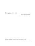
3.1.1 Monitor-based debugging
A monitor-based debugging solution consists of three parts: a front-end, a communication
part and a back-end [10]. The front-end is running at the same machine that the developer
uses when writing and compiling the source code of the program. The communication part
can be any type of media and protocol that can connect the front-end with the back-end. The
monitor executes in the back-end, in the target system, which also is where the debugged
program is executing.
Figure 3. Overview of a monitor-based debugger.
Developer machine
Front-end
Target system
Communication
Back-end
Debugged
program
Besides the media used for communication, monitor-based debugging is a completely
software based solution.
There exist two alternatives as to where the main debugging effort will be performed. The
first option is to run a heavy debug program in the back-end and let the front-end basically act
as a user-interface for this program. This requires that the target system is able to provide a
run-time system for a heavy debugger, and embedded systems normally cannot support a
resource heavy debug program.
The second one is to run a lightweight monitor program at the back-end which acts as a
machine dependent extension to the main debugger program which is running in the frontend. In this way the target system only needs to provide minimal support to the debugging
monitor program. The main debugging is instead done in the front-end, which has a much
better runtime support for it.
The monitor in the back-end could be part of the program that is being debugged or it
could be a separate program. The monitor could also be responsible for downloading the
program that is to be debugged into the target system.
The monitor-based debugger works in the following fashion to perform debugging: there
exist two copies of the program that is being debugged. One copy is used by the front-end and
contains all the debug information of the program. This version is not actually being run, only
used by the front-end to look up information about the program, e.g. which memory address a
certain variable has.
11
The second copy of the program is running in the back-end. This copy could be a stripped
down version without any debug information in it, to make it consume less program memory.
The control of the running program must be transferred to the debugger. This is done by
having the monitor in the back-end generate an exception in the program. The exception
handler transfers control to the monitor, which is controlled remotely by the front-end. The
front-end is controlled by the user of the debugger.
When the user of the debugger has control of the program, some actual debugging work
can be performed. The sequence of events for all debug actions can be seen in Figure 4.
Figure 4. Basic control flow during monitor-based debugging.
User issues a debug command
Front-end uses debug information
to handle the command
Show result of command to the
user
yes
Information sufficient to
handle the command?
no
Order back-end to perform debug
work
Back-end returns the result of the
work to front-end
Let us, for instance, consider the debugging work of reading the value of a variable. This is
initiated by that the user requests the value of the variable. The front-end looks up the address
of the variable by looking in the debug information of the program. This information is not
sufficient to handle the request. The front-end therefore orders the monitor in the back-end to
read the value at the specific memory address. The monitor returns the value of the variable to
the front-end. The front-end now has sufficient information to handle the user request and
shows the value of the variable to the user. The user can then issue a new debug command.
The software to use for the monitor-based debugger could either be bought or an open
source alternative could be used. The software can be platform dependent or platform
independent. However, due to the vast number of different platforms used for embedded
systems, it is almost a requirement that the debugger is platform independent.
12
One of the most common choices to base the monitor-based debugger on is the GNU
Debugger (GDB) [40]. The reason for this is that, as with all software in the GNU family, it is
open source, relative stable and available for a large number of platforms. One notable
monitor-based debugging solution which uses GDB is KGDB [45], the Linux kernel
debugger. In KGDB there is one machine running the Linux kernel (the back-end) and one
machine that is running GDB (the front-end). The communication between the two is either
over a serial line using RS232 or an Ethernet connection.
The biggest advantage when using monitor-based debugging is that it, besides the
communication media, requires no extra hardware. This makes it cheaper than any hardware
based solution and makes it possible to use for any embedded system.
It also is highly flexible because it is a software based solution. This makes it possible to
fine-tune the debugging solution to the system that is being used.
The main disadvantage of a monitor-based debugger is that, as Bannatyne points out [2], it
is intrusive by default because the monitor software needs to reside in on-board memory.
Besides the fact that the monitor program takes up space it also needs to be run. This might
affect the real-time properties of the whole system. The monitor program consistently needs
to communicate with the actual debugger which is controlled by the developer. Because of
this, the debugger monitor itself cannot be halted when breakpoints or similar commands are
issued. This too is a highly intrusive behaviour.
In Sutters implementation of a monitor-based solution [55] he points out that it relies on
the abilities built into the processor to perform debugging. This means that if there is some
part of the system which cannot be accessed by the instruction set supported by the processor
there is no way to debug it.
The time it takes to get a monitor-based solution to work for a particular system could
potentially be much higher compared with a hardware based solution. The reason for this is
that considerable development effort might be needed to adjust the software to the current
system, if it is not carefully designed.
3.1.2 In-Circuit Emulation (ICE)
As mentioned in chapter two, one of the biggest problems with debugging embedded systems
stem from the fact that they are embedded. This often means that there is no viable way to
access and control the internal hardware in the system, which is a requirement for debugging
it in an efficient way.
ICE is a technique in which the system that is to be debugged is emulated by an external
hardware device [13]. This emulation is realised by either replacing the CPU in the system
with the ICE-device or by placing an adaptor on top of the CPU which tri-states it and makes
it possible to use the CPU in the ICE-device instead.
Figure 5. Overview of an ICE debugger.
Target system
Developer machine
Debugger
ICE
CPU
The ICE-device makes internal states of the target system visible. This information is used by
the debugger software running at the developer machine to perform debugging actions. Just
13
like with the monitor-based tool, software at the developer machine is controlling the target
system. The difference is in how this control is achieved and what effect it has on the target
system.
Because the ICE-device emulates the target system it can add high-end debug features that
the target system itself cannot provide. It can also add features that are not immediately
concerned with debugging but nevertheless can be used as debugging aids. This includes
features like code coverage and performance analysis.
ICE also makes it possible to handle real-time issues in a way that is not achievable with
other debug tools. Ganssle gives an example of this [51]: normally it is impossible to single
step an interrupt service routine (ISR) without affecting the behaviour of the system. One
example of this is an ISR that handles incoming data on a serial port. If the transfer rate is not
slower than the time it takes for the developer to single-step through this routine, some data
will be lost as new interrupts will not be handled in time. ICE solves this by capturing the
ISR, without affecting the system behaviour.
Ganssle also points out another situation in which the ICE particularly shines: when using
complex breakpoints. If one would like to break when a particular data-pattern is written to a
particular address, the normal way to implement this would be to single step through the code
until the pattern is recognized, as there is no way the trigger on such a special condition using
the available hardware in the system. The act of single stepping in turns means that the system
speed will be slowed down, which of course affects the real-time properties of the system. If
using ICE however, the hardware emulator can monitor this special condition and trigger on
it, without slowing down the system.
But as O’Keeffe points out [54], the downside with ICE-devices is that they are
considerably more expensive than other debugging solutions.
Hopkins explains [12] that when debugging using ICE it can sometimes be difficult to
know if it is the emulation device that behaves erroneously or the device that is being
debugged. This interferes with one of the most important properties of a debugger according
to Rosenberg [20] – that the user should be able to trust it.
Karcher explains [14] that because of the ever increasing speed in processors in embedded
systems it becomes more and more difficult to emulate the device using a cable and an
adaptor device on the CPU.
Bannatyne discusses a similar problem [2] regarding the evolvement of processors: as the
pin-count on the processor increases it becomes more difficult to physically fit the emulator
adaptor onto the CPU. Space restrictions in the system could also mean that it even is
impossible to fit an adaptor on top of the CPU.
3.1.3 On-chip debugging
On-chip debugging is a technique in which a debugging device is integrated into the system
itself. Through a special debug port on the chip this device can be used to control the
execution of programs running on the processor. The normal way to do this is to connect a
debugger that is running on the developer machine to the on-chip device. That debugger, just
as in the monitor-based and ICE solution, does the major part of the debug work and uses the
on-chip device to realise the debug operations.
14
Figure 6. Overview of an on-chip debugger.
Target system
Developer machine
Debug
port
Debugger
On-chip
debug
device
CPU
The implementation of the on-chip debugger differs from processor to processor [53]. The
debug device has direct access to the internal states of the processor. But what is more
important is that, because the device is an integrated part of the processor, the processor has
been designed with it in mind. Therefore the debug device can monitor and change the state
of the processor without slowing it down and without having any intrusion effects.
There exist standards both for what features the on-chip debug device provides to the
outside and for the debug port that is used for connecting the debugger with the on-chip
device. Of these standards BDM [30] for the on-chip debugger and JTAG [31] for the
interface have been popular choices in the industry. However, some vendors have added
debugging capabilities to their JTAG port and use it for on-chip debugging. JTAG was
originally a standard interface for performing boundary scan testing. Others call their debug
port BDM. This naming could lead to some confusion.
Today the de-facto standard for on-chip debug devices targeting embedded systems is
Nexus 5001 [32] or Nexus for short. The reason a standard is needed is because debugger tool
developers want to support a broad range of processors. If each processor had a different
interface for its on-chip debugging capabilities it would mean that the tool developers would
be required to develop a completely new debugger for each processor. That would make it
impossible for the tool developers to keep up with the pace new processors are introduced.
The Nexus standard is divided into four classes ranging from basic run-time control that
can be found in JTAG based solutions to tracing, watch point triggering and memory
substitution capabilities. The developers of the processor choose which class they should
support. For the basic functionality Nexus uses the JTAG port. For functionality that requires
higher bandwidth an auxiliary port can be added [25].
O’Keeffe [54] lists some of the features which Nexus compliant hardware provides:

Run-time control, i.e. to start and stop the processor, single-step, and modify registers.


Non-intrusive memory access.
Breakpoints, both simple and advanced, i.e. to break on a special condition and not
just when a certain instruction is encountered.
Instruction, program and data trace. Instruction and program trace give the ability to
fully reconstruct the program flow. Data trace allows the debugger to perform realtime analysis of data access.

When tracing using Nexus not all information that is traced needs to be sent to the developer
machine. If for instance the program flow is being traced, only those instructions that interrupt
the normal flow of control are sent [25]. The rest of the instructions can be deduced by the
software debugger by looking at the object code of the program. But even so, the trace
15
requirements imply that a lot of data potentially must be sent to the debugger running at the
developer machine. This leads to high requirements on the connection between the target
system and the developer machine. Potentially the data needs to be buffered and maybe
converted before it is sent. In that case an extra piece of hardware that handles this is required.
Even though a substantial part of the on-chip device solution relies on hardware it still
requires debugger software running at the developer machine. This software is delivered
together with the debugger and adds to the cost of the whole solution. To reduce the costs and
to simplify the design, the debugger software could be replaced by existing open source
alternatives, e.g. GDB. One tool on the market that uses this approach is a debugger called
PEEDI [46]. This debugger will be used as a reference in the evaluation chapter of this report.
The main advantage of using on-chip debugging comes from the fact that it is an integrated
part of the system that is being debugged. Not only will this give good visibility and
controllability of the CPU, but other devices in the system can also be accessed in a nonintrusive way.
Because the debug device is a part of the chip, special care in the design of the chip
concerning debug facilities has been taken. Advanced features such as deep instruction
pipelines, multiple instruction issue and on-chip caches can be accommodated when
debugging, which typically is not possible – even if using advance ICE-devices. In his
comparison [54] between ICE and on-chip debuggers, O’Keeffe explains that high clock
frequencies do not pose the same problem when the debugging device is integrated onto the
chip.
There are downsides with on-chip debuggers too. Integrating the debug device onto the
chip gives extra silicon cost and interface requirements. This makes the system more
expensive and will give a lower yield in production.
O’Keeffe mentions another disadvantage when comparing with ICE: even if on-chip
debuggers can use advanced breakpoints and tracing they are still not as powerful as those
which an ICE-device could create.
3.1.4 On-chip tracing
On-chip tracing is a technique in which real-time data such as program path and data accessed
are non-intrusively recorded, compressed and stored on-chip. This data can be downloaded to
the developer machine and be used for debugging [29]. The program needs only to be run
once and can be analyzed offline, with the same behaviour as if it was running in real-time.
This makes it possible to debug real-time systems in a way that cannot be achieved with
normal run-stop debugging.
Figure 7. Overview of an on-chip tracer.
Target system
Developer machine
Trace
analyzer
software
Trace
storage
On-chip
trace modul
As mentioned in the section about on-chip debugging, the Nexus standard supports tracing.
There are also other tools available that are solely dedicated to tracing [12].
The problem with tracing is the amount of data that is generated. The data can either be
sent directly to the trace analyzer or buffered in trace storage. If the data is to be sent directly
16
to the developer machine, the demands on the bandwidth of the connection becomes very
high. If the data is stored in on-chip memory the cost of the chip increases and the amount of
memory required is high. Consider for instance storing 1 byte of trace data for 512 clock
cycles. That would require 4 Kbit of memory. If the processor is running at 400 MHz, which
means that we can execute one clock cycle in 1 / 400,000,000 seconds, we could store 1.28 µs
of trace data. This is probably not sufficient to catch a bug, so we will need a lot of memory
for the trace storage. Mayer presents a construction technique called emulation extension [18]
that could be used to keep the cost of the system down. In this technique the trace storage is
on an external chip.
The main advantage of on-chip tracing is its non-intrusiveness properties. The system can
be run without interruption and analyzed afterwards. As Thane explains [27], during the
analysis time can be advanced and reversed as seen fit. It is not possible however to directly
observe how mechanical and other external parts that the system interacts with behave when
doing this analysis.
There exist tools that combine both run-stop debugging and tracing, e.g. Nexus devices of
class three or higher. This combination is a powerful, but expensive, tool for debugging
embedded systems.
3.2 Trends on the debug tools market
One trend has been in moving from having hardware do the major part of the debugging work
to letting software handle it. The software uses the debugger hardware to get information
about the processor and the program being run. Ganssle observes [52] that this trend parallels
the overall trend on the embedded market where more and more is being done in software.
Another trend has been the move from ICE solutions to on-chip solutions. Karcher
explains in his outlook of the future of software testing [14] that the reason for this is both that
there is a demand for cheaper solutions but also that the ICE solutions have difficulties with
keeping up with the speed of the systems. This is mainly due to the increased clock
frequencies of the micro controllers. This trend is particularly true for the automotive
industry.
As compilers become more and more advanced it is getting harder for debugger developers
to extract debug information from them. Modern advanced compilers can do sophisticated
optimization that makes the correspondence between machine code of the program and its
high level representation even less tangible than it already is. This could be a serious problem
as it is important that the user trusts the debugging tool. If the debugger reports one view of
the program that does not corresponds to what the user sees, due to that optimization has been
performed, this could damage that trust. Therefore the trend is that there is more and more
cooperation between the compiler writers and the debugger writers.
17
18
4
Selection of a debugging tool
In this chapter the main alternatives previously presented will be compared in the context of
the problem description in the beginning of the report. One of them will be selected as the
base from which a debugger for the system will be built.
The main criterion for the debugging tool considered in this report is that it should require
no extra hardware, besides already existing communication interfaces. The other important
criteria are:


It should be general, i.e. it should be easy to adapt the solution to similar systems.
It should be scalable, i.e. if some parts of the system are evolved it should be easy to
modify the solution so that it still functions.

It should be user-friendly.
Because the system is a real-time system the debugger tool should be as non-intrusive as
possible. “As possible” is a vague and fuzzy requirement. A better requirement might be that
the tool should be able to do debug work in a non-intrusive fashion.
What is common for all the presented alternatives is that they have a debugger program
running at the developer machine that requires assistance from the other parts of the debugger
tool. The difference is in how this assistance is acquired. The ICE, on-chip and trace based
solution all require extra hardware to achieve this.
It would seem then that the choice of debugging tool is simple. If we want a debugger for
an embedded system that requires no extra hardware the only choice is to use a monitorbased solution. However, some properties of the other solutions are desired when realising
the monitor based one. At the same time some properties of the monitor-based solution are
not desirable. These properties will now be discussed.
4.1 Problems and required properties of the selected solution
The biggest problem with the monitor-based solution is that it is intrusive by default. In an
emulated or trace-based solution this problem does not exist. In an on-chip based solution this
problem is minimized due to special hardware.
Instead of emulating the hardware, a simulator could be used in a monitor-based solution.
This is however not feasible because of several reasons:



The development effort of a simulator for a system would be considerable.
It can be very hard mimicking the environment that the system operates in. The effort
to simulate the environment in a sufficient realistic way could outweigh the effort to
build the simulator for the system itself.
If a bug is encountered in the simulated system the user can never be sure if it will
have the same effect in the real system and conversely, if the circumstances that
brought forth a bug in the real system can be recreated in the simulation. This is also
true for the ICE based solutions but less severe, as the program in that case is run on
the same type of hardware as in the real system.
It is however possible to do tracing using a monitor-based solution. After all, tracing is simply
the act of collecting data and use it at a later time to perform debugging. But great care must
be taken when collecting the trace data as to affect the system as little as possible. The frontend must also be able to handle the collected trace data.
19
Another factor related to non-intrusiveness is how to handle breakpoints. Ideally, the state
of the program should be the same before and after a breakpoint, if of course nothing was
changed by the user of the debugger. To implement breakpoints in a monitor-based solution,
investigation is needed to conclude which parts of the system can and which cannot be
stopped and how this affects its properties.
The development time for the monitor-based solution could be far greater compared with
buying a complete debugging tool from some vendor. Therefore care must be taken when
designing the solution as to minimize this. If an existing debugging tool is purchased, some
support for how to install and use it is expected from the user and provided by the vendor.
This is typically not the case when using a monitor and therefore other means must be taken
to assure that the debugging tool is well supported.
4.2 Other considerations
One of the most common uses for a debugger is setting breakpoints, which means that the
program should be suspended. In fact, almost all debugging action requires that the program
is suspended. In the case for embedded systems with no conventional operating system, there
is no easy way to suspend the program without suspending the rest of the system.
But if the system is suspended, there is no way to utilize whatever communication protocol
that the system normally uses. This must be dealt with when implementing the monitor.
Ideally the system has some way to check if the application is running normally or has
stalled, e.g. with a watchdog timer. If the system thinks that the application has stalled it does
some error handling which possibly results in the application being restarted. This must not be
done if the application has stopped responding because of a breakpoint.
4.2.1 The problem with debugging a debugger
A monitor-based debugger is completely software based. In order for it to perform debugging
operations it needs to access special debugging facilities on the processor. Software inevitably
needs to be debugged. In order to debug the monitor-based debugger an existing debugger of
some kind is needed. But this debugger also uses the special debugging facilities on the
processor. Consequently it is not possible to debug the monitor-based debugger when it uses
the debugging facilities.
Instead much more primitive methods are needed, e.g. the use of print-statements (which
for an embedded system means sending data using an external data bus).
This problem could add to the development time of the debugger considerably and should
therefore not be taken lightly.
20
5
Presentation of the selected tool
In this section the general idea behind the monitor-based solution and the components it
builds upon will be presented. This gives the base for understanding its implementation which
is presented in the next chapter. But first let us recapitulate what parts constitute a monitorbased debugger: a front-end debugger running at the developer machine, a back-end debugger
monitor running at the target system and a communication link connecting the two.
5.1 Which debugger to base the solution on
A monitor-based solution is completely software based. In theory it could be based on any
available software debugger, or be written from scratch. Most commercial software
alternatives require the use of a special debug port in the system, i.e. JTAG or Nexus 5001
compatible ports.
Other requirements on the debugger should be that it supports a broad range of
architectures that are used for embedded systems. If the debugger does not support a
particular architecture it should be possible to modify it to change this. That implies that the
debugger should be open source. Add to this the requirement that the debugger itself should
be as bug free as possible, the only viable alternative is GDB which is well tested due to its
large user base. The solution will be based on GDB and GDB is presented in the next section.
Writing the debugger from scratch could also be an alternative. This would give the
required confidence of the capabilities and limitations of the debugger and somewhat make up
for the lack of testing. The whole system could even be designed with debugging capabilities
in mind, leaving room for debugging actions in the real-time scheduler for instance. However,
the development time for a monitor-based solution is already large compared with buying an
existing debugger, even when basing it on an existing debugger. Therefore this will not be
considered as a viable alternative in this report. For those interested in considerations when
writing debuggers from scratch, [20] and [55] are good starting points.
5.2 GNU Debugger (GDB)
5.2.1 Introduction
According to Shebs [22] GDB is one of the most used debuggers in the world. The reason for
this is, amongst others, that it is open source, has a huge user base and, therefore, is well
tested and has support for a large number of platforms. Because it is portable it can be
introduced to new systems as needed. This is crucial for any debugger to be successful on the
embedded market.
GDB has mainly been used to debug applications written in C or C++, but has support for
other languages as well. It can be extended to support new languages. The essential part to
make this extension work is to provide an expression parser for the language as explained in
the implementation description of GDB: GDB Internals [9].
GDB has a quite extensive set of debug actions that it supports. However, the available
ones differ depending on the support from the architecture. In the implementation chapter the
actions that are supported by the target and how they are implemented is presented. A
description of all the commands and their meaning can be found in the GDB manual [24].
In the following sections the overall structure of GDB will be presented. Following this, its
embedded debugging capabilities and different techniques to getting it to run on a new
embedded system will be discussed. In that discussion the system on which GDB runs will be
21
referred to as the host system. The system where the debugged program executes is referred to
as the target system.
5.2.2 Overall structure
GDB consists of three major modules: the user interface, the symbol handling and the target
system handling. This is depicted in Figure 8.
Figure 8. GDB modules.
User
interface
Debugged program
Debug
information
Symbol side
Target side
Hardware
The symbol side handles all the information about the program that can be accessed without
actually running it. This includes symbol table management, source language expression
parsing, display of source code and other things. Essentially, the symbol side of the debugger
can be seen as a part that is consistent over different target types. It is therefore not so
interesting to discuss when specifically looking at debugging embedded systems. As will be
explained later, the symbol side part of GDB will not be run on the target system when
performing embedded debugging.
The target side of GDB is responsible for handling the manipulation of the hardware that
the debugged program is running on. It is this side that is interesting when implementing a
monitor-based debugger.
When performing debugging, the symbol side and the target side work together in the
following fashion: if the user wants to display the value of the variable ARRAY[INDEX + 1],
the symbol side will use the symbol table to look up the address of ARRAY and INDEX. The
target side will fetch the values at those addresses and finally the symbol side will calculate
and display the value to the user.
22
GDB has several user-interfaces. Of these the command line interpreter is the most
common one. Debugging actions are invoked from the user-interface. Doing debug work
should be user-friendly. Typing in commands at a command prompt is considered to be not so
user-friendly by some. Luckily the user-interface can also be implemented in an existing IDE.
This will be discussed more in the implementation chapter.
A monitor-based debugger consists of three parts. When looking at GDB the following
mapping could conceptually be done: the symbol side could be mapped to the front-end and
the target side could be mapped to the back-end. The correspondence to the communication
part is in GDB called the remote debugging protocol.
There are two parts that are needed in order to make GDB support monitor-based
debugging through remote debugging. First of all it has to have support for the architecture
used on the embedded system. If it does not, it needs to be ported to the new architecture.
Secondly, GDB needs to be able to communicate with the remote target and have the target
send responds to debug commands. There are two ways to make this work too: using a GDB
server or creating a remote stub. But first porting of GDB will be discussed.
5.2.3 Porting GDB
According to chapter 16 in [9] there are two aspects in porting GDB to a new architecture:
specifying the machine configuration and implementing required target dependent modules.
Because the system used in the implementation described in this report already is supported
by GDB, this section will only briefly describe what is needed to port GDB.
Specifying the machine configuration is done by modifying existing header files and
configuration scripts in order for GDB to recognize the new architecture.
Implementing the target dependent module is done by giving GDB a description of the
architecture by writing a target architecture definition. The definition tells GDB the layout of
the target processor, e.g. registers, stack and such. A more specific description is sometimes
needed and can be supplied by implementing a target description. This is described in [9].
GDB has support for about 60 embedded architectures [22] and normally both the machine
configuration and the target modules are already included in the GDB distribution. If GDB is
not available for a system, probably not many other tools in the GNU family will be available
either, e.g. a compiler and linker. In that case, an evaluation if the development effort needed
to get the monitor-based solution to work is smaller than the cost to use commercially or
hardware based alternatives is needed.
Besides the architecture description, a set of target vectors need to be implemented. A
target vector is an abstraction that GDB uses to manipulate the target, e.g. fetch register
values and write to memory. A guide to implement a subset of the target vectors needed by
GDB is presented in [7].
When GDB has support for the target system it needs to be cross-compiled on the host
system to create a GDB binary which supports the embedded architecture. Cross-compiling is
the act of building a binary for a processor architecture, using a machine that runs on a
different one. The reason for doing this with GDB is that typically the host system, on which
the program is being developed, does not use the same architecture as the target system.
When GDB has support for the target architecture it needs a way to control the application
running at the target system. This is done by either using a GDB server or writing a GDB
remote stub.
5.2.4 GDB server
GDB server is a control program that GDB can use to control a remote target. It requires the
same operating system support as GDB and is consequently not so useful for embedded
systems with little or no operating system functionality.
23
One might wonder what the reason for using GDB server instead of GDB on the remote
target is. The GDB manual states the following reasons: first of all, GDB server is not as big
as GDB and could be run in more resource constrained environments. Because its code base is
smaller, it also is easier to port GDB server than all of GDB. Secondly, if cross-development
is performed for the embedded system, which typically is the case, it is much more
convenient to use GDB server than GDB for debugging. And, as discussed in the beginning of
the report, there might not even be a way to interface GDB on the embedded system in a
conventional way, e.g. using a keyboard and a monitor.
Because the system in the implementation described in this report does not have the means
to run GDB server it will not be used in the implementation.
5.2.5 GDB remote stub
A remote stub is a relatively small piece of code that is linked together with the program that
is to be debugged. The stub implements the target side of the remote protocol in GDB, i.e. it
implements the monitor in the back-end when using GDB as a front-end in a monitor-based
debugger. The GDB distribution comes with some example stubs for a couple of systems, but
otherwise the stub needs to be written from scratch. The implementation of a remote stub will
be presented in the implementation chapter of this report.
In his presentation of the remote protocol that GDB uses [6], Gatliff explains that there
exist several alternatives as how to get the program with the remote stub onto the system so
that GDB can start to communicate with the target. One way is to put a small application into
non-volatile memory which can respond to GDB when it wishes to upload the program to be
debugged onto the system.
Another way is to place the whole stub in the non-volatile memory.
If the program is downloaded to the target outside of GDBs control, it makes debugging
more cumbersome for the user as the debugging becomes a two step exercise. First the
program needs to be downloaded and then GDB needs to be started. If, on the other hand,
GDB is responsible for downloading the program, the user simply needs to start GDB to start
the debugging session.
However, it is not always desirable or feasible to let GDB handle this. If the target system
initially were developed without considering remote debugging, a way to download programs
already exists. In this case it is not desirable to change this into letting GDB be responsible for
downloading the program. Consider what should be done if GDB is not to be run but a
program should be downloaded. In this case there would exist two ways for the program to be
downloaded. This could lead to unnecessarily added complexity of the system.
In the case of the system used for the implementation described in this report, there is no
separation of the program that is run on the system and the system itself, once the binary file
for the program is produced. The programs are linked together with the system; there is no
system which could receive a program which GDB could download.
Chapter 17 in the GDB manual lists the minimal requirements to get the stub to work:




C-runtime support must be available at the target system.
There must exist a way to download the stub to the target.
A routine handle_exceptions. This routine handles the communication with GDB at
the host. It is this routine that implements all the code for controlling the target.
A routine set_debug_traps. This routine must set up the target system so that
handle_exceptions is called when an exception occurs. Consequently,
handle_exceptions is never called explicitly.
24


In order for GDB at the host to get the initial control of the application, i.e. for
handle_exceptions to be called, a breakpoint must be inserted into the application.
The routine breakpoint does this. However, if other means exist to cause an
exception this could instead be used. One way might be if there exists an interrupt
button at the target which causes an exception. Another way might be if the reception
of a message on the communication link used causes an exception. In that case, the
initial connect message from GDB will cause an exception and the control of the
application will be implicitly transferred to GDB.
Two routines, getDebugChar and setDebugChar, which the stub uses to receive and
send debug commands.
The above names for the routines are what are used in the stubs that come with the official
GDB distribution. Note however that this naming convention is only what is recommended in
the GDB documentation. The GDB at the host does not need to know how it gets the required
debug information from the target. The only thing that is required is that when GDB sends a
specific command, it should get a corresponding response from the target.
How the correspondence to these routines is implemented is presented in the
implementation chapter.
Ideally, from the point of view of GDB running at the host, there should be nothing that
gives away how the remote stub is implemented.
5.2.6 The GDB remote serial protocol (RSP)
A complete description of RSP can be found in appendix D of the GDB manual. It is this
protocol that GDB at the front-end uses to communicate with the GDB stub (or server) at the
back-end.
RSP is a relatively simple protocol for sending ASCII-encoded characters over a serial
line. The reason that the characters in RSP are ASCII-encoded is that it should be easy for a
human to communicate with the target stub, using for instance a PC-terminal.
Messages in RSP are called packets.
Figure 9. A RSP packet.
$
… payload ...
#
checksum
A packet begins with a $. Following this any number of characters could come. These
characters represent the data payload. The end of the payload is indicated by #. After the
payload terminator is a checksum. The checksum is calculated as the sum of the payload
modulo 256. The checksum is sent as two ASCII characters representing the hexadecimal
value of the checksum, i.e. if the checksum value is 0xEF, ASCII 101, 102 should be sent
(which is 0x65 0x66).
RSP is a request/reply protocol. It sends a command (request) and receives a response
(reply). When it has received the reply it can send the next command. All request/reply
sessions are initiated by GDB.
When either GDB or the target receives a packet it should always begin with
acknowledging it by sending + (ACK), or requesting a resend by sending – (NAK). Reasons
for resending could either be an ill-formed packet or that the checksum calculation failed.
To save space, the data payload can be run length encoded. By this it is meant that a
sequence of the same character is replaced by one instance of the character followed by a
repeat count.
GDB supports a lot of commands, but the stub is not required to implement all of them.
Only those listed in Table 1 are required.
25
GDB Command
G
G
M
M
C
S
Table 1. Required GDB commands.
Action
Read general registers.
Write general registers.
Read memory.
Write memory.
Continue.
Single step.
Consequently it is the commands in Table 1 that the initial development effort of the
command processing at the stub should be focused on. GDB also provides the opportunity to
use custom commands that only the stub understands. GDB at the front-end only shows the
response of the custom command to the user and does not do any command processing of its
own. This is a way to extend GDB and customize it for a particular system without recompiling GDB at the front-end.
Here is a short example of how the communication using RSP could look like:
GDB -> $g#67
Target -> +$123456789abcdef0#62
GDB sends the g command. The checksum is in this case the hexadecimal value of g, as it is
the only data in the payload.
The target responds by first sending +, acknowledging that it has received the packet
correctly. It then sends the hexadecimal value of all its registers as the data payload. If we
assume that the size of the general purpose registers at the target is 32 bits, the values of these
would be 0x12345678 and 0x9abcdef0. This can be seen by the ASCII string
123456789abcdef0 in the payload, which simply is the hexadecimal representation of all the
registers concatenated into one string. The checksum is the decimal sum of the data payload
(49 + 50 + 51 + 52 + 53 + 54 + 55 + 56 + 57 + 97 + 98 + 99 + 100 + 101 +
102 + 48 = 1122) % 256, which gives the value 98. 98 are represented as 62 in
hexadecimal.
The importance of the checksum is questionable. If the checksum is wrong it could both
indicate that the payload is corrupt or that the checksum itself has been corrupted. There is no
way to tell, so the whole message needs to be retransmitted.
If an ACK has not showed up after some time (which can be defined by the user of GDB)
it is undefined if the ACK or the data itself was lost. This makes sense in some cases as some
commands (e.g. STOP) could stop the target for an unknown amount of time and it is
therefore impossible to know how long it should take for the target to respond. In other cases
however it would be desirable to have a resend mechanism.
The design aim with RSP has been to put the responsibility of lost packets and similar
incidents at the target and not clutter the protocol with it. The reason for this is that the target
should decide what to do in these cases. In some systems it could be desirable to shut down
the debugging session if a packet is lost. The developer of the stub could see to this. In other
systems it could be desirable to skip the lost packet and act upon the next one instead. Stubs
could be implemented to handle this too.
GDB has built in support for TCP (and UDP) and RS232 to be used when doing remote
communication. If the target system does not support one of these, some kind of proxy
program must be written in order for GDB and the target to be able to communicate. The
implementation of such a program will be discussed in the implementation chapter.
26
5.3 Overview of the solution
With a good understanding of what debugger we will use for the solution and its capabilities
we can summarize and give an overview picture of all the parts in the solution and how they
are connected.
Figure 10. Overview of the implemented debugger.
Target system
Front-end
IDE
Communication
GDB
Proxy
RSP
Back-end
GDB stub
The front-end of the debugger is implemented by GDB. An existing version of GDB
compiled for the architecture of the target system will be used. The user-interface to GDB,
and thereby to the front-end, is an existing IDE on the developer machine. The back-end of
the debugger is implemented by a GDB stub that will be written from scratch. GDB and the
stub communicate using the GDB remote serial protocol, and there is a proxy program
between GDB in the front-end and the target system.
27
28
6
Implementation of the selected tool
In this chapter the implementation of the monitor-based debugger will be presented. The
chapter is started with a presentation of the system the debugger will be implemented in, and
where in the system the different parts of the debugger reside. After this comes the description
of the implementation of the front-end, the communication link and the back-end.
6.1 System description
From the introduction chapter we recall the layered view of the system, as seen in Figure 11.
These layers will be described in this section. Of course, the description is only valid for the
particular system used in the implementation described in this report. However, a
corresponding description can be derived for many other systems, e.g. AUTOSAR [37] based
systems, and therefore the discussion in this section is interesting for anyone who is about to
implement a monitor-based debugger.
Figure 11. System that the debugger will be implemented in.
APPLICATION
SBSW
EBSW
Common Platform
SMAL
EMAL
HW
6.1.1 Application
This is the layer containing the actual applications that are run in the system. They interface
the hardware through functions provided by Common Platform.
6.1.2 SBSW (Standard Basic Software)
This module contains software that is common to all control units that Common Platform
supports. The functions in this layer can be seen and used by the applications. The aim with
the design of Common Platform is to place as much of the functionality as possible in SBSW.
Basically all software that is not dependent on the hardware used can and should be placed in
this module. By doing this, porting Common Platform to new hardware is easier and quicker
as all the functionality in SBSW can be re-used.
6.1.3 EBSW (ECU Specific Basic Software)
This module contains software that is common for a specific control unit, e.g. the control unit
for the engine that Common Platform supports. This includes, for instance, descriptions of
29
how the different electronic devices in the control unit are connected to the microcontroller. If
the mappings are changed for a specific control unit, only this module needs to be updated.
6.1.4 EMAL (ECU Specific Microcontroller Abstraction Layer)
EMAL is the layer that provides drivers and utilities to access the hardware. EMAL is specific
to the hardware in the control unit and needs to be rewritten if Common Platform is to be used
on a new hardware. Besides EMAL there are also functions from the microcontroller vendor
which are placed in MMAL. Conceptually both these layers are on the same abstraction layer.
6.1.5 SMAL (Standardized Microcontroller Abstraction Layer)
SMAL is an interface between SBSW and EMAL, i.e. the interface that SBSW goes through
to access the hardware. SMAL interfaces are standardized for all ECUs that are using
Common Platform.
6.1.6 HW (Hardware)
Normally this is the actual hardware of the control unit, but a simulator could also be used.
The layered approach will, when used properly, reduce the development effort needed
when introducing new hardware. Only hardware specific functions are needed to be
redeveloped. The rest of the layers should be able to be used as they are.
A debug monitor should accommodate to this design philosophy, i.e. only the parts of the
debugger that are hardware dependent should be needed to be changed when the debugger is
used on new hardware. This will make the debugger implementation scalable.
6.2 Where the debugger comes in
Given the system description in the previous section the different parts of the debugger will
be integrated in the system according to Figure 12. The abbreviations in the figure are
explained in this section.
Figure 12. Debugger placement in the system.
Host
Target
DSBSW
IDE
DSMAL
Application layer
Program
GDB
TCP/IP
GDB to
CAN
CAN
SBSW
SMAL
DEMAL
EMAL
Program
HW
GDB stub
30
EBSW
6.2.1 Program
The program exists in two copies. One contains the debug information and is used by GDB at
the host. The other is a striped down version without debugging information running at the
target. Note that the program at the host is not running; it is only used by GDB to get debug
information. What also can be seen from the above figure is the fact that the program that is
running at the target has no knowledge of that it is being debugged nor has the debug stub any
direct contact with the program. All the interactions between GDB and the program are with
the host side version of it.
It should also be noted that the platform itself can be debugged using the debugger,
because the application and the platform are linked together into one binary file. The
debugger cannot however be used to debug itself.
6.2.2 GDB
The GNU Debugger running at the host. Together with the IDE this is the front-end part of
the debugger.
6.2.3 TCP/IP
TCP/IP is the communication protocol that GDB utilises to communicate with the GDB stub
at the target machine. As previously described GDB only supports this protocol and RS232.
6.2.4 GDB to CAN
GDB uses the TCP/IP protocol to communicate with the remote stub. Because GDB has
support for this protocol but the target system typically has not, a conversion program is
needed; GDB to CAN. This makes the stub independent of the GDB version used. The
implementation of the proxy program will be explained in detail in the communication section
of this chapter.
6.2.5 CAN
CAN is the protocol that is used to communicate with the target over a serial bus. This
protocol is explained in more detail in the communication section of this chapter.
6.2.6 DSBSW (Debugger SBSW)
This is the high-level part of the GDB stub. It does everything that is not directly dependent of
the hardware. This includes:

Receiving and sending data on the CAN-bus, i.e. receiving and sending GDB remote
serial protocol packets.


Parsing incoming packets and doing high-level handling of the data payload.
Given a data payload, constructing outgoing packets.
DSBSW mostly consists of functionality for handling packets. If we recall how a monitorbased debugger works this is not so surprising. It is the debugger at the front-end that does
most of the work. When it has done all it can it asks the stub in the back-end for help. One big
part of being able to aid the front-end is to know what it wants. That is what DSBSW figures
out.
When DSBSW has done all it can with the data payload, it calls corresponding debugging
functions in DSMAL.
31
6.2.7 DSMAL (Debugger SMAL)
This is the part of the debug stubs that maps from general debug operations called from
DSBSW to specific debug operations for the hardware used, i.e. functions defined in
DEMAL.
6.2.8 DEMAL (Debugger EMAL)
In this part of the debug stub the actual debugging work is done. DEMAL accesses the
hardware to perform debug operations on request of DSBSW, which in turn performs them on
request of GDB at the front-end. Some actions produce a response payload, e.g. reading
memory at a specified address. Other actions do not produce an explicit payload response, e.g.
setting a breakpoint. In those cases DEMAL only tells DSBSW if the debug actions were
successfully performed or not.
The implementation of DEMAL and DSBSW will be presented in the back-end section of
this chapter. The implementation of DSMAL will not be discussed as it simply is an interface
between DEMAL and DSBSW.
6.3 Implementation of the front-end
The front-end consists of GDB and a user-interface to it. GDB was described in the previous
chapter. As was also mentioned in that chapter the standard user-interface for GDB is a
command line interpreter. Because this is not considered to be so user-friendly, a graphical
user-interface (GUI) will be used in the implementation. There exist several alternatives for
this.
6.3.1 GUI for the front-end
Graphical front-ends could be divided into two categories: the ones that provide a complete
development environment and the ones that just act as a graphical user interface that lies on
top of GDB. Of the later kind a further breakdown could be done by looking at GUIs that are
completely separate from GDB (e.g. DDD [47]) and GUIs that is built together with GDB
(e.g. Insight [39]).
The goal with the implementation is to provide a solution that is as user-friendly as
possible. Therefore, to separate the GUI that the user uses to write code and the GUI the user
uses to debug the code is not a good idea. The front-end should be one that integrates all the
functions the user needs in the same interface, i.e. an IDE.
Users have different opinions on just what should be included in the IDE. A requirement
on the IDE should therefore be that it is highly customizable, both when it comes to how to
arrange the actual functionality in the IDE but also with regard to plugin support. And of
course, the IDE must support GDB as its debugger. A candidate that fulfils all these
requirements is Eclipse CDT [43], but other IDEs could, of course, be used if they support
GDB and the user prefers them. Eclipse CDT is a development environment for developing C
and C++ applications. It has a source editor and gives the user the possibility to both
customize which build suite (i.e. which compiler and linker) to use and which debugger. It
also has support for extending the IDE by writing plugins for it. In fact, CDT is a plugin for a
general IDE for development called Eclipse [42].
6.3.2 Building GDB for the front-end
To cross-compile GDB for the target architecture the following steps need to be performed:

Download the GDB sources. They can be found at [40].
32



The sources are built by using the GNU build system. This means that we first call the
configure script that is provided with the sources. The configure parameter is the
architecture which should be specified in the form --target=ARCHITECTUREVENDOR-OS. In the case of the implementation described in this report the architecture
is PowerPC [33], the vendor is unknown (at least to GDB) and there is no operating
system. Instead of the operating system we provide the application binary interface
used. This tells GDB how it should interact with the underlying hardware of the
architecture. PowerPC uses EABI (Embedded Application Binary Interface) [35].
Therefore the target parameter used is --target=powerpc-unknown-eabi. GDB does
not provide any easy way to list all its supported target combinations but provides a
script, config.sub, which can be used to guess which available architectures there are.
For instance we could guess that there is support for Sun OS by issuing config.sub
sun4. In that case we would get the response sparc-sun-sunos4.1.1 and could use
that as our target parameter.
Besides providing the target parameter we should enable the simulator for the
architecture, if it exists. For PowerPC this is done with --enable-sim-powerpc.
When we have configured the installation we build it by simply using the GNU tool
make.
6.3.3 Customizing GDB
GDB has support for the architecture of the processor in the system the implementation this
report describes deals with. For other systems GDB might not have support at all in which
case GDB must be extended and re-compiled. But even though GDB has support for a
particular architecture it does not mean that GDB knows about every system that uses that
architecture. For instance, the system described in this report is built on a board called
Freescale MPC5566 [41]. That board is based on the PowerPC processor architecture but adds
additional registers and modules. Compilers for PowerPC can still be used for the board
because the additions do not change it in any fundamental way, but GDB has no knowledge
of these additions.
From a user perspective, it could be interesting to be able to look at the extra registers
when debugging. But it would be cumbersome to extend GDB by re-compiling it to support
these registers; any future changes in GDB could, potentially, break the extensions that are
added if they are not incorporated into the official GDB distribution. The official GDB
distribution would become very large if it were to include every architecture variant there
exists. As Hanson explains in his paper about an alternative debugger [11], the bulk of GDB
already mostly consists of code for supporting different variants of platforms and processors.
There is however a way to extend GDB for minor architecture variants such as these without
re-compiling it.
This customization comes in the form of the Target Description protocol, which is
described in appendix F of the GDB manual [24]. This protocol defines a format in which
target features can be described. For instance, a custom register set could be defined in an
XML file and GDB would in that case use that register set when it reads and writes the target
register file, instead of the default one.
GDB can obtain this custom description in two ways. Either it can request it from the
target through the remote serial protocol command qXfer or the user of GDB can supply it
with the set tdesc filename command.
If the target supplies the description it is both easier to maintain the description, e.g. if the
register set is changed, the target automatically should generate a new description, and also
makes it easier for the user of GDB.
33
However, to generate an XML file at the target might not be trivial. Further on, the target
description could be set in some start-up file that GDB uses. In that case there is no extra
burden on the user.
Note that GDB needs to be linked together with the Expat XML parser library [38] in order
to be able to use target descriptions.
Another way to customize GDB without re-compiling it is to use the monitor command.
According to the GDB user manual this allows for sending arbitrary commands directly to the
GDB stub. Since GDB does not care about the commands it sends like this, this command is a
way to extend GDB. For instance this could be used as a way to gather system specific
information from the stub and displaying it to the user.
To communicate with the stub, remote serial protocol packets must be sent using the CANbus. As mentioned in the previous chapter, GDB only has support for TCP and RS232
communication. GDB could be extended to support CAN, but the same discussion as above
goes for this; it would mean that the extension would be required to be integrated in the
official distribution of GDB or else future releases could potentially break it. For some it
might be worth the extra effort to get a communication extension accepted into the official
GDB branch. There are many advantages with this, the biggest one probably being that the
extension would be carefully reviewed and tested by a lot of people. From a user perspective
the big advantage with this would be that there would be no difference using GDB for the
new system with using it with a system that supports RS232 or TCP communication. In the
implementation this report describes however, this will not be done.
Another way to be able to use CAN is to write an external proxy program. That program is
run on the same machine that GDB is. This will be the approach that is used in the
implementation this report describes and the implementation of the proxy will be described in
the next section.
6.4 Implementation of the communication link
The system that the solution has been implemented on uses CAN as the communication
protocol between the target and the host. Here follows a short description of that protocol.
6.4.1 CAN (Control Area Network)
CAN [34] is a broadcast, differential serial bus protocol. Only one node can transmit a
message at a time. It has mainly been used for connecting devices in automotive vehicles, but
can, of course, be used for other applications as well.
The reason that CAN is used in automotive applications is that it is often required that
certain communication does not take longer than some maximum time. For instance, one
device could be the break actuators and the other the control unit that controls the breaks. If
the control unit controls the break by sending a message on the CAN-bus it is not desirable
for the message to arrive too late.
CAN solves this problem by giving the messages priorities. If several devices want to send
messages at the same time, the one with the highest priority will be sent first. According to
Burns and Wellings in their book about real-time systems [4], it can be shown that certain
messages will always arrive in time if the identifiers are properly assigned.
The downside with having a priority scheme is that it limits the transmission speed. For
CAN the bound on the transmission is dependent on the length of the wires used for the bus.
Therefore, it is best suited for connecting devices that are close to each other, e.g. the control
units in an automotive vehicle.
Messages in CAN are called frames. A frame consists of the identifier, the data message,
checksum and flags.
34
6.4.2 Interfacing GDB using CAN
There are at least three approaches to solve the communication of GDB not only with CAN,
but with any communication protocol that is used by the target system.
The first approach has already been discussed and is to extend GDB itself.
The second approach is to go the other way around and add support for one of the two
protocols GDB supports at the target system. This would require adding new hardware to the
system, which does not make the solution feasible in the general case.
The third alternative is to keep both GDB and the target system as unchanged as possible
with regard to their communication interfaces. To achieve this, a program that converts from
the communication protocol used by GDB to the communication protocol used by the target is
needed.
A CAN frame can hold eight bytes of payload data, but other protocols could use bigger or
smaller packets. Therefore, in order to make the proxy general, GDB packets should be able
to be of any size.
6.4.3 Proxy implementation
The UML class view in Figure 13 is used to describe the proxy implementation.
Figure 13. Proxy implementation class view.
«datatype»
comDataType
dataType:comDataType
iCom
#recvFunctionPointer
+switchOrder()
+toCharBuffer()
+read()
+write()
+registerRecvFunction()
+send()
targetCom
GDBCom
#parserFunctionPointer
+aSyncReceive()
dataType:comDataType
targetCANComImpl
#recvFunctionPointer
+aSyncReceive()
targetCANCom
GDBSocketCom
-generalCANTypes
-implementor
+initCAN()
+exitCAN()
-port
-implementor
+initSocket()
+setCallback()
+send()
targetCANComWinImpl
dataType:comDataType
GDBSocketComImpl
#recvFunctionPointer
#parserFunctionPointer
+setCallbacks()
+send()
GDBSocketComWinImpl
The goal with the implementation of the proxy has been to make it independent of both how it
interfaces GDB which is running at the front-end and how it interfaces the target connection.
To realise this, the proxy has been designed based on a variant of the Bridge design pattern
[8], which will be explained now.
The proxy is divided into two parts: the connection to the target and the connection to
GDB. Both these connections are required to implement the abstract interface iCom. This
interface requires that there exists a send-operation and a way to register an asynchronous
receive-operation, which will be called when a message is received on the respective
connection. The reason the receive operation is in the form of a callback is that it should be
allowed for incoming messages to come at any time and that these messages should be
35
handled automatically by the callback function. An alternative to using the callback-based
approach would have been to have a receive function which would be polled. This would
have been less efficient.
targetCom and GDBCom are two other abstract interfaces that inherit from iCom and add
specific requirements on the interface that is needed when communicating with the target and
GDB, respectively. For the target side not much is added, only a function that should be
called when data is asynchronously received. For GDB a pointer to a GDB packet parser
function is also required to be supplied. The reason for this is that typically some conversion
is needed when sending the data from GDB onto the target connection. In the case of the
implementation the target connection is limited to sending eights bytes at a time, i.e. the
maximum amount of payload data for the CAN-bus. Therefore a parser is needed that divides
the data stream from GDB into eight byte chunks.
The data type used throughout the whole proxy is a template parameter with some
requirements on the operations supported on the type used. Having the type as a template
parameter through the whole design makes it more general.
The type should support I/O operations in the same way that the built in types in whatever
language that is used. In the implementation described in this report C++ was used, therefore
the type was required to support the stream operators (<< and >>).
The type should also have an operation for switching the byte order of its internal
representation. This is required if the driver responsible for sending data onto the
communication link and the target system does not use the same byte ordering.
Lastly, the type should be able to give its internal representation as an array of characters.
This makes it easier to use the type together with legacy software; much in the same way as
most types in e.g. C++ has a to_char operation or an implicit conversion for this.
Both the target connection and the GDB connection could be implemented in different
ways. For the GDB connection there exists the alternative between a serial connection and a
TCP connection. For the target connection the alternatives include basically any
communication protocol there is. Furthermore, the platform used at the developer machine
where the proxy is running places additional constraints on the implementation of the
connections, i.e. how to use a communication protocol differs depending on the operating
system used.
Changing either the platform or the connections should require as few changes in the
overall proxy design as possible. This is achieved by separating the implementation of the
connections from their interfaces and is where the Bridge design pattern is used. This design
pattern consists of two parts: the abstraction and the implementor. The abstraction defines the
operations that are needed, but uses an implementor object to execute them. The implementor
in turn is further divided into concrete implementors. What happens when an operation in the
abstraction is called is that the work is delegated to be performed by the concrete
implementor. In this way the same abstraction could use different implementors.
In our particular implementation the CAN-bus has been used as the target connection and
TCP as the GDB connection. targetCANCom is the abstraction for the target connection.
targetCANComImpl is an implementor and targetCANComWinImpl is a concrete
implementation for using a USB CAN driver in Windows. What all this means is that when
the send-operation is called at targetCANCom it will use targetCANComWinImpl to actually
perform a send operation. The GDB connection is designed in the same way.
The benefit from this design comes in its generality. If one would like to implement the
CAN connection in another way, e.g. for the UNIX platform instead, the only thing required
to change would be to add a targetCANComUnixImpl and make sure that this was called
instead. If one would like to implement a serial target connection instead, one would add a
36
targetSerialCom and a corresponding implementor. The same goes for the GDB connection.
This modularity makes the solution easier to adapt for new systems.
The difference with this design and the design in the original Bridge pattern is that in that
one there are refined abstractions for every abstraction. Each refined abstraction can use every
concrete implementor. This makes no sense in the front-end, as this would mean that, for
instance, a targetCANCom could use a targetSerialComImpl to send its messages. The
downside is that this also means that more work is needed when adding a new target
connection, as both the abstraction and the implementor are required to be re-written.
Nevertheless, it is clear where in the design the connection should be added, which makes the
proxy modular.
To summarize. What a developer of a proxy for a new target and/or a new connection type
to GDB needs to provide is the following:
1. A function that handles received data from the target.
2. A function that handles received data from GDB.
3. A function that does any necessary processing of data from GDB before it can be sent to
the target.
4. A type for representing the data sent which has the necessary operations.
5. An abstraction and implementor for the connection used.
6.4.4 The communication chain in the proxy
To get a better understanding of the proxy it can be advantageous to look at how a packet is
transferred from GDB to the target and vice versa.
37
Figure 14. Communication chain in the proxy.
GDB
sendMsg
sendMsg
Socket library
GDBSocketCom->send
GDBaSyncRecvFunction
GDBSocketCom
GDB to CAN proxy
targetCANCom
targetASyncRecvFunction
targetCANCom->send
CAN library
sendMsg
sendMsg
Target
GDBsocketCom uses a socket library to handle messages to and from GDB. targetCANCom
uses a CAN library to do the same with the target.
In a typical debug session GDB issues a send command to send a debug command to the
remote target. The remote target, in this case, is the local host (the developer machine on
which GDB and the proxy is running). This call is intercepted by GDBSocketCom, which uses
a listening socket to capture the communication. GDBSocketCom uses the callback function
registered by the proxy to process the message. In the normal case the message is parsed
using the above mentioned parser function and then just sent on by issuing the send operation
in targetCANCom. Finally, targetCANCom uses a CAN library to send the message to the
target. When the target responds, a corresponding call chain is invoked.
38
The important thing with this call chain is that GDB does not know that its messages are
intercepted by the proxy. GDB thinks that the target is actually running at the local host. This
gives the proxy the opportunity to do some command processing before the command reaches
the target. It is even possible for the proxy to not send the message to the target at all, but
instead fake a response. This could be useful in some situations. For instance, GDB
commands, that the proxy knows that the target does not support, could be intercepted already
in the proxy. This saves time, but, at the same time, creates a dependency between the proxy
and the target that might not be wanted.
6.5 Implementation of the back-end
The back-end consists of the GDB stub. The implementation of the stub will be described in
this section. Some example stubs are included in the GDB distribution. The source code for
these can be used to get some inspiration of how to write a stub. However, those stubs rely too
much on the processor and the specific functionality to be of any use as a general stub
implementation which this implementation tries to be.
The control flow in the debug stub during a whole debug session can be described by the
following graph:
39
Figure 15. Control flow in the debugger back-end.
Init high level debugger, DSBSW. Register callbacks in
the low level handler.
Init low level debugger, DEMAL.
Wait for debug interrupt.
Do low level handling of debug interrupt.
Call high level debug handler.
Do high level handling of debug interrupt.
Call low level handler.
Hardware
support
needed?
yes
no
Debug work
done?
no
yes
As with all other modules in Common Platform, the debugger stub is initialized when the
system is started. When DSBSW is performing its initialization it registers some callbacks in
DEMAL. The reason for this is that it is always DEMAL that is called by the interrupt system
when a debug interrupt has occurred. As we shall see in the next section, all debug work
originates from debug interrupts generated by the hardware. When the low level handling is
done, DEMAL uses the callback hooks to call the high level handler.
6.5.1 Debug interrupts
As was mentioned in chapter two, seizing control of the program being debugged is done
differently depending on if the program being debugged is on the same machine as the
40
debugger or not. If they are, the debugger controls the program by system calls, i.e. it controls
the program with the help of the operating system.
If the program is run on another machine the debug stub seizes control of it. The way it
does this is by registering an interrupt handler for a special kind of interrupt that is called
debug interrupt in some processors [41].
The way to register an interrupt handler differs from processor to processor. Normally the
processor has a number of interrupts it can generate. The interrupts are prioritized. This means
that the interrupt handlers could in turn be interrupted if an interrupt with a higher priority
was generated. Debug interrupts normally have the highest priority of all interrupts in the
processor. The reason for this is that it should be possible to debug other interrupt handlers as
well.
Associated with the different interrupts is a table in the processors internal memory. Each
type of interrupt has an entry in this table. The entries consist of pointers to interrupt handlers,
i.e. addresses to memory locations where the code for the interrupt handlers is. When an
interrupt occurs, the processor will look into the table and call the corresponding interrupt
handler. It is the interrupt handler that handles the interrupt, i.e. does some processing and
then gives back control to the entity that was interrupted.
The stub, therefore, needs to do two things to seize control of the processor. It needs to
provide a function that handles debug interrupts and it needs to write the address of this
function into the processor interrupt table.
One question remains and that is how debug interrupts are generated. This too differs from
processor to processor, but normally the processor can generate debug interrupts for at least
the most fundamental debug action: triggering a breakpoint. The implementation of
breakpoints will be discussed in more detail shortly, but basically a breakpoint is implemented
by writing a breakpoint address to a special breakpoint register in the processor. The entity
that is executing in the processor is the program we want to debug. Therefore the breakpoint
address will be the address of an instruction in this program. When the processor is about to
execute the instruction at this address it will generate a debug interrupt. This will transfer
control to the debug stub through the debug interrupt handler. The stub can transfer this
control to GDB at the front-end. Once GDB has seized control of the program it can control
its execution by sending commands to the stub. The implementation of these commands will
be discussed shortly.
The above described process of seizing control of a running program in a remote system
can be visualized by the following UML sequence diagram:
41
Figure 16. Sequence diagram for debug interrupts.
Program
Debug stub
System
Debug interrupt handler
Register debug interrupt handler
Write address of program in debug register
System init done, program is started
Debug interrupt generated some time later
Control is transfered to debug stub, program suspended
The debug stub wants to seize control of the running program; therefore it registers a debug
interrupt handler and writes an address in the program into a breakpoint register. At the same
time the rest of the system is initialized. When this is done the program is started. Sometime
after this, the processor will fetch the instruction at the address the debug stub wrote, and the
processor will recognize that this address also is in the breakpoint register, and generate a
debug interrupt. The debug interrupt handler will be called and can transfer control of the
whole system to the debug stub.
If there are no concepts like debug interrupts and breakpoint registers in the processor used
for a particular system, the above mentioned procedure can in some cases still be used to seize
control of the program. In that case an interrupt for handling illegal instructions can be used.
Instead of a breakpoint register an illegal instruction can be written into the program memory
of the running program. When the processor encounters the illegal instruction, the interrupt is
generated and control of the program is transferred to the stub.
6.5.2 Correspondence to required stub routines
Recall that GDB requires some minimal routines to get a debugging stub working at the
target. Here is the correspondence to these routines in the implemented solution.
6.5.2.1 handle_exception
This routine corresponds to the low level debug interrupt handler in DEMAL together with
the high level debug handler in DSBSW. The low level handler takes care of the hardware
generated debug interrupt and then calls the high level handler. The high level handler is the
workhorse of the debug stub and is the routine that delegates all debug work on behalf of
GDB at the front-end. The pseudo code for this routine is:
42
do
{
parseIncomingGDBPacket()
if (payload.GDBCommand == continue)
{
debugSessionDone = true
}
else
{
callCommandHandler(payload.GDBCommand)
}
} while (debugSessionDone != true)
The high level handler consists of a command processing loop. In each iteration of this loop
any new incoming GDB packet is parsed. As long as the command in the packet is not
continue, which means that GDB is done with its debug work for now and wants the program
to resume its normal execution, the command handler for the specific command is called and
the loop continues. The implementation of each GDB command will be discussed shortly.
When this function returns, control will be returned to the program and execution is
resumed at the place the program was interrupted.
6.5.2.2 set_debug_trap
This routine should generate the initial debug interrupt. As we have seen in the sequence
diagram in Figure 16, this is done by having the debug stub write an address in the program to
a breakpoint register or equivalent. The question is which address in the program should be
used.
One approach would be to put the address at the beginning of the main routine in the
program. That would mean that the program is suspended directly when it starts with its
normal execution. Another approach would be to use the address of some low level init
routine in the system platform. The problem with both of these approaches is that the debug
stub does not know when, or even if, GDB at the front-end will ever request to take control of
the system. If no debugging is to be done the program would still be suspended, which is not
desirable.
Another way is to set a debug exception to occur when the target receives the first packet
from GDB, i.e. use the address of the function that receives incoming GDB packets. When the
first GDB packet has been received the target can be certain that GDB wants to take control of
the system. As long as GDB does not try to seize control, the program execution will continue
as normal. The downside with this is that the user of the debugger cannot single step the
program from its first point of execution.
The approach used in the implementation this report describes was to use the latter
alternative.
6.5.2.3 getDebugChar and setDebugChar
These two functions correspond to the back-end process of handling incoming and outgoing
GDB packets which will now be explained.
6.5.2.4 Handle incoming debug packets
As already described, GDB packets are sent as CAN-frames to the target system. In the
system platform for the implementation this report describes, there already exist routines for
handling incoming CAN-frames. These routines can be set up in such a way that a specific
routine is called when a CAN-frame with a certain identifier is received. That routine would
be the routine in the debug stub that handles incoming packets and the identifier would be the
43
one the proxy uses when sending GDB packets. In other systems similar frameworks probably
exist or could be implemented by using a header for all incoming data packets to the system.
The routine in the stub simply places incoming data from GDB in a queue.
In order for the packets to be handled, they need to be parsed from the incoming queue.
Parsing could be initiated before the whole GDB packet has been received. In fact, without
parsing the packet there is no easy way to know if the whole packet has been received.
Therefore the parser must keep track of how much of the packet has been parsed. When a
packet has been parsed, it is considered to be removed from the queue. For some GDB packet
the queue could look like in Figure 17.
Figure 17. GDB packet queue.
Queue
Message 1
Message 2
Message
3
Already
parsed
Front
Back
GDB Packet
In the above queue the GDB packet consists of three messages. The last message was padded
(the black part) in order for the packet to fill a complete number of messages. This makes the
design of the parser easier, but wastes space in the queue. The first message in the packet has
already been parsed (the striped part). The front pointer points to where the parsing should
continue. The back pointer points to where the next message should be inserted into the
queue.
The parsing procedure is explained with pseudo code. Recall the structure of a GDB
packet; starts with $, payload, #, and end with a checksum.
44
if (in the middle of parsing a packet)
{
while (Queue.front.message[i] != ’#’)
{
payload += Queue.front.message[i]
if (i at end of message)
{
front++
i = 0
return ParseNotDone
}
else
{
i++
}
}
calculateChecksum()
if (checksum OK)
{
removePacketFromQueue()
return ParseSuccesful
}
else
{
removePacketFromQueue()
return ParseFailed
}
}
else
{
if (Queue.front.message[0] = ‘$’)
{
ContinueParsingPacket()
}
else
{
removePacketFromQueue()
return ParseFailed
}
}
The front pointer indicates where the oldest message in the packet, which is to say the
message that should be parsed from the queue, begins. If we are in the middle of parsing a
packet we continue by reading each character until we find the end of packet marker or find
the end of the message in which case we return and will continue parsing later, probably in
the next iteration of the debug handler loop. If we found the end of packet marker we
calculate the checksum, and if it is correct the parsing was successful otherwise it failed. In
either case we remove the whole packet from the queue, making room for a new one.
If we are on the verge of parsing a new packet, we first check if we really received a new
packet. If we did, we continue parsing the packet as described above.
An alternative to the queue system, where the packets are stored as a number of messages
in a queue containing a fixed number of messages, would be to skip the queue abstraction
completely and just store the incoming frames in a byte buffer. In this buffer it would be
needed to keep track of where the next incoming frame should be stored and where the next
parsing operation should continue from. The implementation of this might be easier than a
queue system. The drawback is that the abstraction level is lowered from message level to
byte level.
45
What happens when a new message arrives when the queue is full, and what happens if
packets are lost, is explained in the section about the send and receive FSMs, 6.5.3.
One big question with handling the incoming packets remains though. When we are
receiving packets from GDB we are in a debug session, which means that the program and the
rest of the system are suspended. If the system is suspended we normally cannot handle
incoming packets as this is handled by functions in the system that cannot be run as long as
we are in a debug session. In the implementation this report describes this is solved by
explicitly polling the CAN hardware for incoming GDB packets, in each iteration of the
debug handler loop.
6.5.2.5 Handle outgoing packets
Handling of outgoing packets is quite simple. The outgoing payload has already been
constructed by the command handler for the packet that the response is intended for. What
needs to be added to the payload is the start of packet marker, end of packet marker and the
checksum.
Hexadecimal values are sent as the corresponding ASCII character, which requires that
values in the payload need to be converted before they are sent.
How the checksum is handled requires some explanation. Consider for instance that the
payload aabb is sent. When the checksum for this is calculated the payload is seen as binary
data, i.e. aabb is the same as AABB. 0xA, 0xA, 0xB, 0xB would be added together in the
calculation and not the ASCII coded values of either aabb or AABB.
The checksum however, is sent as the ASCII coded values of the two hexadecimal
numbers that represent the checksum. This could potentially lead to a mismatch if the target
sent aa as the checksum (ASCII 97, 97) and GDB calculated it as AA (ASCII 65, 65). Luckily
GDB handles this by converting the checksum characters using the formula:
char a
if ((a >= '0') && (a <= '9'))
{
return (a - '0')
}
else if ((a >= 'a') && (a <= 'f'))
{
return (a - 'a' + 10)
}
else if ((a >= 'A') && (a <= 'F'))
{
return (a - 'A' + 10)
}
The stub does the same when it checks the checksum during packet parsing.
Because the outgoing packet is a response to a packet sent by GDB an ACK should be sent
before the response packet. That could be done separately or by simply appending + at the
beginning of the response packet. GDB will see this as two packets: first the special packet
ACK and then the response packet.
When the outgoing packet is constructed it is placed in an outgoing packet queue. The
content of this queue is sent out on the CAN-bus, eight byte at a time.
6.5.3 Send and receive Finite State Machines (FSMs)
One of the key aspects for the robustness and success of the debug stub is to have a solid
infrastructure for sending and receiving packets.
46
To get a good understanding about how to handle lost and corrupt GDB packets during a
debug session, GDBs send and receive FSM will be explained in this section. This description
can be derived by looking at source code file remote.c in the GDB sources. From this
description the corresponding FSMs for the debug stub are derived and limitations of the
protocol and their implications on remote debugging are discussed.
The notation for the transitions in these FSM is Cause for transition / action taken. “-“ as
an action represents that nothing else is done besides changing state.
6.5.3.1 GDB send FSM
Figure 18. GDB send FSM.
NAK received / Re-send
Send / -
Wait for send
command
Wait for ACK
Timeout / Re-send and timeoutCount++
ACK or timeoutCount > 3 / Old packet received / Ignore data and ACK
GDB starts to send a GDB packet when someone on a higher level at the front-end (which is
to say the part of GDB that constructs outgoing GDB packets) issues a send command. GDB
then sends the whole packet and begins waiting for an ACK from the receiver, which would
imply that the packet has been received correctly.
If GDB receives a NAK instead of an ACK it means that the receiver has received the
packet, but that something was wrong with it. GDB re-sends the packet in this case and will
continue to do so a potentially infinite amount of times if the target always responds with
NAK. This implies that it is not a good idea for the target to send NAKs in respond to packets
that it does not support, as this will hang the debug session. Instead the target should send
ACK and an empty packet as response, which means that the packet which GDB sent is not
supported. GDB can then terminate the debug session in a proper way.
If GDB does not receive a response after a certain amount of time has passed it re-sends
the packet and increments a counter. If the counter is greater than three, GDB gives up
sending the packet and moves on. Alas, GDB will try to re-send a packet which it gets no
response for three times.
If GDB receives a packet when it is waiting for an ACK it assumes that this is an old
packet that the receiver has not received an ACK for and therefore has re-sent it. GDB ignores
this packet as it assumes that it already has received it, but sends an ACK in response in order
to get the target to move on.
47
6.5.3.2 GDB receive FSM
Figure 19. GDB receive FSM.
Start received / Timeout / NAK and timeoutCount++
Wait for start of
packet
Wait for rest of
packet
Rest received or timeoutCount > 3 / ACK
When GDB has sent a packet it begins to wait for the start of the response packet. GDB can
wait for the start of the response indefinitely. The reason for this is that GDB has no way of
knowing how long it should take for the stub to act upon a received packet. The packet could,
for instance, be a continue command which simply says that the target should continue its
execution until it stops of its own, e.g. because it has encountered a breakpoint, and then
inform GDB the reason for stopping. The stopping point could be the next instruction the
target executes or it might never be reached.
It is important to distinguish between this situation and the situation in the send FSM
where GDB also can wait indefinitely and its impact it has on the usability of the debugging
tool. In the case of the send FSM, it would for the user look like GDB has hanged for no
apparent reason, because in the normal case the user does not inspect every packet sent during
a debugging session. In the receive situation, however, the user would not get the false
impression that GDB has hanged, as the user is very much aware of what it means by sending
e.g. the continue command.
When GDB eventually receives the start of a packet it assumes that the rest will follow in a
rapid fashion. If it does not, GDB sends a NAK and increments a timeout counter. It tries to
receive the rest of the packet three times. If it has not done so after these three attempts it
gives up and pretends that the packet was received correctly. This is one of the situations
where the debugging session could get out of synch, i.e. GDB and the back-end have different
views of what packets have been sent and received. Potentially, this could lead to that the
debugging session is terminated by GDB.
48
6.5.3.3 Back-end send FSM
Figure 20. Back-end send FSM.
NAK received / Re-send
Send / -
Wait for send
command
Wait for ACK
ACK / Old packet received / ACK
The send FSM for the stub resembles the one in GDB quite much. When a send command has
been issued the stub waits for ACK from GDB. If it receives an NAK it will try to re-send the
packet. No timeouts are needed at the back-end as GDB will eventually give up and send an
ACK. This means that the debugging session could get out of synch, but at least the target
will not hang.
If the back-end receives an old packet when it is waiting for an ACK it makes the same
assumptions that GDB does and responds by sending an ACK.
6.5.3.4 Back-end receive FSM
Figure 21. Back-end receive FSM.
Start received / -
Junk received / NAK
Wait for start of
packet
Start received / NAK
Rest received / if Checksum = OK send ACK else send NAK
49
Wait for rest of
packet
If the stub receives anything (besides the special packet ACK and NAK) but the start of a
packet when it is waiting for a new packet it assumes that the packet was corrupted and
responds with a NAK.
When the start has been received, the stub will wait for the rest of the packet. It makes no
assumptions about how long it should take to receive the rest of it. However, if the stub
receives a new packet while it is waiting for the rest of the current one, it assumes that the rest
of the current packet was lost and that GDB has re-sent the packet. It then sends a NAK and
begins waiting for a new packet; to be sure that it receives it properly. GDB will give up the
current packet after three timeouts and move on to the next one. This could lead to the
debugging session to get out of synch. Again, the stub leaves timeout handling to GDB and
trades the potential risk of hanging for the risk of getting out of synch.
Regardless of how the checksum calculation fared, the stub starts to wait for a new packet
when it is done. If the checksum failed, GDB will receive a NAK and re-send the packet and
the target will try to receive the packet again.
6.5.3.5 Problems with the FSMs
A couple of situations where the debugging session could get out of synch have already been
mentioned and there probably exist even more cases where this could happen.
Surely a more elaborated protocol could be implemented at the stub, in order to reduce the
situations where this could happen. However, debugging a remote system can never be one
hundred percent safe as long as the connection used could corrupt the packets sent. A
consideration between the effort spent making the stub smart enough to juggle itself out of
problematic situations and the risk of getting corrupted packets must be made.
In the typical case the debugging is done over a single connection, i.e. no routers and
unknown networks exist between GDB and the stub. In these cases the rather simple protocol
explained above should suffice.
The user of a remote debugging tool must have a mindset which says that debugging
remote systems is different from debugging normal systems. In some cases the session could
get out of synch and needs to be restarted. GDB also helps a lot with this. It can in most cases
decide if the session needs to be terminated or if it can continue even though some packets
have been lost.
Another thing to consider is the potential of buffer overflows. Could packets at the stub
stack in the incoming and outgoing queues and potentially lead to them getting full?
Remember that resources in embedded systems are limited.
The answer to this is no. The stub never receives a new packet until it has received and
ACKed the old one. At this point the packet is removed from the queue. The same goes for
the outgoing packet queue. The stub never puts a new packet in the outgoing queue until it has
received an ACK for the old one, at which point it is removed from the queue. This gives the
opportunity to calculate the maximum sizes of the queues as they are the same as the
maximum size of incoming and outgoing packets. This maximum size of packets typically is
realised when sending all the register values back and forth. The important thing is that the
size is known by the developer of the stub, and therefore the queues can be statically allocated
with no risk of them overflowing.
6.5.4 Command processing at the back-end
When the infrastructure for handling GDB packets is in place and when there exists a way to
generate and handed debug interrupts in the stub, the one thing left is to handle the debug
commands that are sent. It is the command handlers that do the actual debug work on behalf
of GDB. The command processing in the stub can be broken down into the steps in Figure 22.
50
The command processing is integrated with the send and receive FSMs described in the
previous section.
Figure 22. Command processing at the back-end.
Receive packet
Parse packet
no
Whole packet
parsed?
yes
Handle command
Construct response packet
Send packet
6.5.4.1 Receive packet
The packet is received and placed in an incoming packet queue.
6.5.4.2 Parse packet
The packet is parsed, as described in the previous section. The parsing could go on for some
iterations if the whole packet has not been received yet.
6.5.4.3 Handle command
In this step the GDB command is handled. The first step in this is to check which command
was sent to know which command handler should be called. All GDB commands are
represented with one ASCII character, so this is done by simply looking at the first character
in the payload.
In these routine further parsing might be needed. For instance, if the command was M
(write memory), further parsing is needed to conclude at which address the writing should be
done and what value should be written. Other commands, like the g command (read general
51
registers), requires no extra parsing as all the information is given by the command itself. The
implementation of each command handler will be discussed in detail in the next section.
When all the information required to handle the command has been gathered, the required
action is taken.
As mentioned in the section about the proxy, some packet processing could be done
already at the proxy. This fact raises the discussion as to whether all the command processing
should be done at the back-end or not. The proxy typically both has greater processing power,
bigger memory etc, but also better opportunities to relay processing information to the user.
It is therefore tempting to let the proxy do as much as possible. Conceptually, everything
that the back-end does not need to see, e.g. commands that it does not support, commands that
are poorly formatted, could be handled by the proxy. But this would break the modularisation.
The proxy should be able to be used with any back-end. It should simply be a communication
relay between GDB and the target. If the proxy does any command processing, it is instantly
tightly coupled with the back-end.
One could argue that the proxy could at least check for corrupt packets. This is not
dependent of the back-end. But as the proxy runs at the same computer as GDB, it is much
more likely that any corruption of packets occurs when it is sent from the proxy to the backend and not when it is sent from one process to another on the same computer.
6.5.4.4 Construct response packet
The packet is constructed in the way described in the previous section.
6.5.4.5 Send packet
In this stage the packet that is to be sent lies in the outgoing queue. Therefore it is simply sent.
6.5.5 Command handlers
In this section the implementation of a number of GDB commands and the action that should
be taken by the stub when GDB sends them are explained. Only those commands
implemented by the stub that this report describes are detailed. With each command an
example of the packets exchanged is provided, where GDB issues the command and the target
provides a typical response.
Remember that GDB minimally requires that the g, G, m, M, c, s, ? and k commands are
supported by the stub. GDB itself implements far more commands and a complete list can be
found in the GDB manual.
The reason for a stub to not implement a command could either be that the command is not
applicable, e.g. commands concerning thread handling in a stub with no operating system, or
that the command simply is a more elaborate way of achieving something another command
does, e.g. writing memory by sending the data in binary compared to writing the memory by
sending the data as ASCII-characters. Other reasons could be that the development effort to
implement a command simply is too great compared to the benefit it would give to the user of
the debugger.
6.5.5.1 ‘g’ command (read registers)
The values of the registers declared by GDB in the file gdb/regformat/reg-xyz.dat should be
sent to GDB. The registers should be sent in the order declared in the file and the individual
bytes of the registers should be sent in target byte order. GDB uses this information together
with the architecture description to determine and display the values of the registers to the
user. Each byte of the register value should be described as two hex digits. This means, for
instance, that the byte 0x00 should be sent as 0x30 0x30 (00 ASCII).
52
When GDB issues this command it typically is because the program has been suspended
(for instance due to a breakpoint) and GDB needs the register values to e.g. do a stack
backtrace or determine the value of the program counter. When the program is suspended,
code in the debug stub is executing. This means that the stub cannot simply read out the
register values as they are in the actual processor registers and send them to GDB, because
these values will not be the same as they were when the program initially has suspended due
to the debug interrupt. The register values GDB want are the ones that were saved when the
interrupt was taken. The procedure for saving the working registers differs from processor to
processor. In some processors the values are saved on the stack, e.g. the processor [33] used
for the implementation this report describes.
Regardless where the register values are saved, the stub must be able to fetch them
whenever GDB issues this command. In the stub in the implementation described in this
report the registers are saved on the stack. Therefore, an approach to fetching the registers
from the stack will be explained here.
To read the values from the stack the stack pointer as it was when the debug interrupt was
taken must be saved. One solution to this would be to save it in a dedicated register, for
instance a debug register, during debug interrupts and use this to find the correct values on the
stack. Another approach is to use a global variable that can be accessed both from the routine
that handles context saving during interrupts and the debug stub.
The g command could require that, compared to other commands, a lot of data is sent. On a
32-bit machine each register would be sent as 8 bytes of data. If the machine is RISC based
there are a lot of general purpose registers.
Example:
GDB -> $g#67
Target -> +$00055fe0...a3b321f3#94
GDB sends the command and the target responds by sending all the register values.
6.5.5.2 ‘G’ command (write general registers)
GDB uses this command to send new values for all the registers. The values are sent in the
same order as the stub sends them in the g command. The same discussion as for the g
command goes here. The new register values that are sent should be used by the debugged
program when it is resumed and not by the debug stub. Therefore, the values need to be
written to the place where the registers are saved, i.e. on the stack.
Example:
GDB -> $G#00055fe0...4001fe10#54
Target -> +$OK#9a
GDB sends the values of all the registers and the target responds by sending OK, if the register
values were successfully written. Otherwise, the target should respond by sending an error
packet: Exx.
6.5.5.3 ‘m’ command (read memory)
GDB sends this command together with an address to start reading from and a length in bytes
specifying how much to read. The stub needs to parse out this information from the
command, which means that the stub must convert the address and length sent as ASCIIcharacters into an actual address value that can be used to access the memory. This
53
conversion is needed in more commands, so it is a good idea to write a function that does this.
The stubs provided in the GDB distribution have examples of how to implement this function.
The stub should respond by sending each byte of memory as the two ASCII values
representing the two hex digits.
Example:
GDB -> $m102054,4#f9
Target -> +$898dd246#0d
GDB wants to know the value of the data starting at memory location 0x102053 with length
4. The target responds by sending the value.
6.5.5.4 ‘M’ command (write memory)
This is the opposite of the previous command. GDB sends the data that the stub should write
into memory, at the address provided in the command.
If the target cannot use hardware to set breakpoints, GDB will use this command to write a
TRAP or an illegal instruction at the breakpoint address in order to generate breakpoints.
GDB also uses this command to change e.g. the values of variables during runtime.
In some systems this command cannot be supported fully. The implementation described
in this report is one of them. The reason for not supporting this command could be that part of
the program lies in memory which is not modifiable during run-time. An example of such a
memory would be flash memory. A possible work around to this is discussed in the evaluation
chapter of this report.
In the implementation described in this report the program memory is in flash and the data
memory is in RAM. Therefore, this command is partly supported by allowing writing to those
addresses that are in RAM.
Not supporting this command, of course, limits the capabilities of GDB. GDB cannot
perform all its actions without it and, because of this, it is one of the commands that the GDB
manual lists as required. But even so, if the target system has support for hardware assisted
breakpoints, a lot of debugging work can still be done. If the target neither has support for this
command nor can use hardware breakpoints, GDB as a debugging tool is reduced to a mean
to suspend the processor once and then read out program information.
Example:
GDB -> $M40006104,4:000002ad#5d
Target -> +$OK#9a
GDB sends the memory address to write at (0x40006104), how much to write (4 bytes) and
the value to write (0x000002ad). The target responds with OK if the memory was written
successfully.
6.5.5.5 ‘c’ command (continue)
This command tells the stub that the processor should continue with its normal execution, i.e.
that it should return control to the program being debugged. Additionally, an address can be
provided with this command, specifying that the program should resume at this address. In
that case, the program counter value stored during the debug interrupt should be changed so
that the program will resume from this address and not from what it was at when the debug
interrupt occurred.
54
The implementation of this command could be simple; just return from the high level
debug handler.
After this command is sent, the debugging session could or could not continue. This
depends on if the target encounters any breakpoints. If it does it should sent a packet to GDB
saying why it stopped. These packets are called stop reply packets. In a stop reply packet the
reason the program stopped its execution and some additional information can be sent.
The additional information can be used to send the PC and stack pointer value to GDB as
GDB always will request this information when the program has stopped. By providing this
information in the stop reply packet and not forcing GDB to explicitly ask for it, the time it
takes for some debug actions, single stepping in particular, can significantly be decreased.
The reason for this is that e.g. single stepping will trigger a lot of breakpoints. If GDB must
send additional commands to query about the PC and stack pointer at each breakpoint the
time to perform the whole debug action will increase.
Example:
GDB -> $c#63
Target -> +$T0501:4001fd70;20:001040b4;#17
GDB asks the target to continue. Sometimes later the target stops and tells GDB why it did so,
and provides some additional information. The reason the target stopped is that it received
signal 05 (SIGTRAP). The additional information it provides is the stack pointer (register
0x01) value (0x4001fd70) and the PC (register 0x20) value (0x001040b4). The values for the
signal and the register numbers are only valid for the processor architecture of the system that
the implementation described in this report uses. For other systems one must look in the
architecture description in GDB for that particular system, to find the values that should be
used.
6.5.5.6 ‘s’ command (single step)
This command tells the processor to execute one instruction and then stop the execution and
give back control to GDB. Additionally, an address could be provided with this command,
specifying that the program should be single stepped starting from this address.
This command could be implemented in several ways. One would be to set a breakpoint at
the instruction after the PC address the program will resume at. The problem with this is that
it is hard for the debug stub to know what this address is. For instance, the instruction which
the program resumes at could be a conditional jump instruction.
Another way is to use hardware support for single stepping. In the implementation
described in this report there exists an instruction complete interrupt. Using this, the
implementation of this command is quite straight forward. Activate the interrupt and resume
program execution. After on instruction this interrupt will be taken. The interrupt controller
for this interrupt then needs to transfer control to the debug interrupt handler.
Care must be taken to specifically activate the interrupt just before the program execution
continues and then deactivate the interrupt as soon as one instruction has been taken. The
reason for this is that we do not want the stub to trigger this interrupt by itself; it is the
debugged program that should trigger it.
Rosenberg states [20] that the act of single stepping a program could change its behaviour
on some processors. When single stepping, the instructions are processed by the processor in
strictly program order as opposed to normal execution where the processor could do out of
order execution.
When the stub has single stepped the program it should send a stop reply packet to GDB.
55
Single stepping is slow when using the instruction complete interrupt approach, even when
providing the extra stop reply information described above. If the user wants to single step
one statement at the source code level this could potentially lead to hundreds of instruction
complete events being generated, as one source level statement could correspond to a lot of
machine level instructions. To speed-up single stepping, GDB can in some cases use
breakpoints instead of asking the stub to single step the program. If, for instance, GDB knows
the address of the next source level statement that will be executed, a breakpoint could be
inserted there and the target could run at full speed up to that point.
Example:
GDB -> $s#73
Target -> +$T0501:4001fd70;20:001040b4;#17
GDB sends the s command. The target will single step the program one instruction and then
suspend it, and inform GDB why the target stopped.
6.5.5.7 ‘?’ command (indicate the reason the target halted)
This is a command that is sent by GDB to find out why the program has stopped its normal
execution. The stub must respond by sending a stop reply packet.
Example:
GDB -> $?#3f
Target -> +$T0501:4001fd70;20:001040b4;#17
GDB typically sends the ? command during start up of a debug session, when the program
has stopped but not due to a breakpoint set by GDB.
6.5.5.8 ‘k’ command (kill target)
This command is sent by GDB when the user terminates the debugging session. The response
action is not well defined. Either the program could be shut down, which for an embedded
system typically means that the whole system is shut down, or it could just continue with its
normal execution.
The approach used in the implementation that this report describes was to reset the system,
which means that the program is re-started and thereafter running as normal.
Example:
GDB -> $k#6b
Target -> +
GDB tells the target to kill the program. The target simply ACK this command, and after this
the debug session is ended.
6.5.5.9 0x03 command (remote_interrupt)
If GDB wants to interrupt the program when it is running, 0x03 will be sent. If the stub wants
to support this command a breakpoint must always be set in the function that handles
reception of GDB packets, in the same way the initial debug interrupt is handled. However,
when the command has been received the breakpoint should be removed. Otherwise every
56
packet that GDB sends after this would generate a new debug interrupt. The breakpoint can be
re-inserted when GDB sends the continue command.
Example:
GDB -> 0x03
Target -> +$T0501:4001fd70;20:001040b4;#17
The remote interrupt command is special in that it is not a normal RSP packet, only a
hexadecimal value. The reason for this is that the command really is an interrupt signal, which
should be processed by the systems ordinary signal handler. If no such handler exists in the
system the interrupt signal can be treated as an ordinary RSP packet. This was done in the
implementation this report describes. When the debugged program has been interrupted it also
has stopped, and the target should tell GDB why it did so.
6.5.5.10 Breakpoint commands
A breakpoint is a point in a program at which the normal execution should be stopped and the
program suspended, so that the program state can be inspected and, possibly, modified. It is
crucial that the state before and after the program suspended is un-altered, except for any
changes that explicitly are made by the user of the debugger. In the implementation that this
report describes this was dealt with by suspending all the timers in the system during debug
interrupts.
The breakpoint command is the fundamental action that a debugger must be able to
perform. To implement a breakpoint, three things conceptually have to be done:
1. The instruction at the point where the breakpoint should be inserted must be saved.
2. Instead of the instruction, a breakpoint instruction should be inserted. When this
instruction is executed the program stops.
3. Before the program continues, the old instruction needs to be re-inserted and the
breakpoint removed to make sure that the program semantics is not changed when the
program resumes.
There exist several kinds of breakpoints. Memory, or software, breakpoints are breakpoints
that are implemented by writing a breakpoint instruction into memory. The instruction
typically is a TRAP or illegal instruction. Anything that can suspend the program and transfer
control to a debug interrupt handler will do. This way of implementing breakpoints can only
be used when the program memory is writeable during runtime. That is not the case for the
implementation in this report and therefore hardware breakpoints have been used.
Hardware breakpoints are breakpoints that do not rely on the ability to write into memory
but instead uses hardware facilities in the processor to pause the execution at the point where
the breakpoint is inserted. In the implementation described in this report, hardware
breakpoints are supported by special debug registers in the processor. When an address is
placed in these registers, the processor will suspend the execution if it tries to execute an
instruction from this address. The above listed steps are what GDB does if the target does not
support hardware assisted breakpoints.
Using hardware breakpoints is a more simple approach compared to using software
breakpoints, but the amount of available hardware breakpoint registers in a processor is
limited. Another advantage according to Rosenberg [20] with using hardware breakpoints is
57
that it avoids issues with instructions caches as no extra instructions are inserted in the
program memory.
Watchpoints are like breakpoints, but instead of breaking when a certain instruction is
executed the program pauses when certain data addresses are written to or read from. Just like
with breakpoints, watchpoints can be implemented by using hardware facilities if they are
available. Hardware assisted watchpoints are to prefer because software watchpoints in GDB
are very slow, as stated in its implementation description [9].
There are issues to consider when using watchpoints. Watchpoints for local variables can
only be used when the variable is in scope. If the variable goes out of scope GDB will delete
the watchpoint, as the watched variable does not exist any longer. If a variable that is watched
is larger than what can be monitored by all the watchpoint registers available, GDB will use
software watchpoints instead. When watching a local variable it could be that the variable is
in a register. In that case too, GDB will be forced to use software watchpoints as registers
cannot be watched by using hardware watchpoints. GDB cannot use software watchpoints for
read and access watchpoints. The reason for this is that GDB in that case would need to watch
the execution of every instruction, as every instruction potentially could read the watched
variable. When GDB uses software watchpoints for write watchpoints, it only needs to check
if the value of the variable has changed after each source level single step.
When using hardware breakpoints and hardware watchpoints the stub must be able to keep
track of which breakpoint registers are in use and which are free and which registers should
be cleared when GDB requests to remove a breakpoint. This is because GDB does not know
how many breakpoint registers there are, in fact at the start of a debug session GDB does not
even know if it is possible to use hardware assisted breakpoints. It finds out this by trial and
error.
GDB supports all the mentioned breakpoints types through its zx and Zx commands, where
x tells the stub which type of breakpoint that should be inserted.
GDB supports conditional breakpoints but the stub is not involved in this. GDB
implements them by setting an unconditional breakpoint and at each breakpoint check the
condition. The fact that GDB uses unconditional breakpoints and stops the program several
times is not directly visible to the user, but it slows down execution. If one would like fast
unconditional breakpoints a technique called run time code patching [3] could be used.
Example:
GDB ->
Target
GDB ->
Target
GDB ->
Target
$Z0,1040b4,4#71
-> +$OK#9a
$c#63
-> +$T0501:4001fc50;20:001040b4;#14
$z0,1040b4,4#91
-> +$OK#9a
GDB tells the target to set a hardware breakpoint (Z0) at address 0x1040b4. Additionally
GDB provides the length (4 bytes) of the breakpoint instruction. This should be used if the
target implements the breakpoint by writing to the program memory. The target responds by
sending OK if the breakpoint was set successfully. GDB then tells the target to continue.
Sometime later the breakpoint is hit and the target tells GDB why the program stopped.
Because the breakpoint has been hit, GDB asks the target to remove it (z0). Again, the target
should respond by sending OK if the breakpoint was removed successfully.
One might wonder why GDB removes the breakpoint; there is nothing telling GDB at this
point if the user wants the target to hit the same breakpoint again or not. The answer to this is
that GDB only removes the breakpoint temporarily. If the user does not tell GDB to remove
58
it, it will be re-inserted before GDB sends the next continue command. The reason GDB does
this is that, in order for the program execution to be continued with the breakpoint in place,
the breakpoint must be removed and the program single stepped past it. Otherwise the
program will only hit the same breakpoint again when it continues, and the program execution
will not advance.
The sequence of packets exchanged for the watchpoint commands follows the same
pattern. The difference is the stop reply packet that should be sent, which should tell GDB
that a watchpoint, and not a breakpoint, has been triggered.
6.5.5.11 Tracepoint commands
As mentioned earlier in the report, one of the main difficulties with debugging embedded
systems is to do it in a non-intrusive way. As also has been mentioned, one way to handle this
is to implement tracing. This could be done in a naïve way by inserting print statements in the
program that will report the values of certain variables that we are interested in. There are two
main downsides to this approach. Inserting print statements in a program is cumbersome and
re-compiling of the program is required each time we either remove or add a print statement.
The second thing is that executing print statements is by itself something that affects the state
of the program. At the very least, it would mean an extra function call during the execution.
This could be crucial if we would like to do detailed timing analysis of the program
execution. But even more so, print statements imply I/O-operations and these typically are
much slower than just the time to do a function call, especially for embedded systems where
I/O means sending things using external communication links.
GDB uses a more sophisticated approach to tracing called Tracepoints [38, 52]. In this
technique, GDB tells the program to trace certain information at certain points during its
execution. The program does this and when it is done with its execution it sends the collected
trace information to GDB. GDB can use this information to let the user do debugging work in
the normal way, but as if it were done when the program were executing at nearly full speed.
GDB calls the act of tracing a trace experiment.
The way the target conceptually implements this is with breakpoints. For each line in the
program where GDB has requested there to be a tracepoint a breakpoint is inserted. When the
program reaches this point, a debug interrupt is generated, just like when a normal breakpoint
is hit. The difference is what the target does when it hits this breakpoint: it simply stores
whatever information GDB has requested in a trace buffer in memory and then returns from
the interrupt. This is much faster than the time it would take to store the information with an
I/O-operation. Also, Scottow suggests [21] that if the routines that collect the data are short
and compiled inline, they will have a very small invasive effect on the program that is being
traced and the information collected during the trace experiment should be close to its real
value, i.e. the value it would have had during normal execution.
When GDB requests information from the trace experiment, say the value of variable, the
target reads it from the trace buffer in memory instead of reading its current value.
The limitation with tracing is space. All the information needs to be stored in memory and
memory is a sparse resource in embedded systems. Because of this the tracepoint
implementation for the stub will be limited to collecting variables. In GDB no such limit
exists. This will be discussed more in the evaluation chapter of the report.
6.5.5.12 Tracepoint implementation
The structure for handling tracepoints can be described using the schematics in Figure 23.
59
Figure 23. Tracepoint implementation.
Tracepoint
breakAddress
numberOfPasses
activeFrame
001
001 + length 002
002 + length
Value1
Value2
Frame1
Frame2
00n
...
00n + length
ValueN
Variable1
Variable2
FrameN
length
.
.
.
VariableM
A tracepoint has a breakAddress which is the address at which the program should pause and
collect variables. It keeps track of how many passes it should collect variable data, i.e. how
many times the breakpoint address should be hit during a trace experiment. For each pass the
value of the variable is saved in a new frame. This is the approach GDB uses when it request
trace experiment data; it requests to read data from a particular frame. Values can be saved in
N different frames where N is the maximum number of passes that a tracepoint experiment
can be run for. Finally, a tracepoint has a buffer for each variable it should trace and it can
trace M different variables.
Each variable has a length and a buffer containing the values that have been collected for it
during the tracepoint experiment. Each value in the buffer corresponds to a frame and each
value takes up length bytes in the buffer. If GDB wants to know the value of variable Y during
frame X the variable buffer would be indexed with Y and the variables value buffer would be
indexed by X * length.
Besides storing the value for a variable at its base address, the value stored at each address
up to its base address plus its length is also stored. The reason for this is the way GDB
handles variables that lie adjacent in memory. Let us take the example with two variables A
and B that have addresses 0 and 4, where variable A has length 4 and variable B has length 2.
If GDB where to handle these as two separate variables when it requested which variables
should be collected during a tracepoint experiment, everything would be fine. However, GDB
tries to be extra clever, so instead it says that it would like to collect one variable with length
6 and start address 0. The trouble begins when GDB wants to read back the value of the
variables. When it does this it first requests to read variable A at address 0 and with length 4.
This is fine. But then it asks to read back variable B at address 4 and with length 2. If we
would not store all the addresses from the base address up to the variables length we would be
lost by now because we would have no information of a variable with address 2.
Therefore, to read back the value of a variable we first find the correct buffer as mentioned
above. We then do a linear search in this buffer for an address that matches the one GDB
requested.
The support for displaying the collected information is powerful in GDB. Using a C-like
scripting language the information could for instance be generated with a while loop that goes
through all the collected frames and print out them to the console. Add to this the ability to
log the output in the console to a text file and this information could quite easily be shared
with other programs, e.g. print it as comma-separated file and use it to generate a graph. More
information about how to do this can be found in the GDB manual.
60
Example:
GDB -> $QTinit#59
Target -> +$OK#9a
GDB -> $QTDP:1:00104218:E:0:a-#1f
Target -> +$OK#9a
GDB -> $QTDP:-1:00104218:M-1,40006104,4#9b
Target -> +$OK#9a
GDB ->
$QTro:00040000,00040010:00040010,00040020:00040020,00040030:00040030,000400
40:00
040070,00040080:00040080,00040090:00040090,000400a0:000400a0,000400b0:00040
0b0,000400c0:000400c0
,00040100:00040100,00040110:00040110,00040120:00040120,00040124:00040250,00
0402ac:00040500,00130
ff8#b3
Target -> +$OK#9a
GDB -> $QTStart#b3
Target -> +$OK#9a
GDB begins a tracepoint experiment by telling the target to initialize the tracepoint ( QTinit).
GDB then tells the target to create a new tracepoint (QTDP) at address the 0x00104218, with a
passcount of 0xa. After this GDB tells the target which variables to collect (0x40005104) and
the length of the variables (0x4). In this example there is only one variable, but more variables
can be sent by GDB and their information would in that case be concatenated in the same
packet.
The QTro packet tells the target which memory regions it should read the current values
from when GDB requests the collected tracepoint information. Typically, this corresponds to
read-only memory regions, e.g. program memory. As the memory is read-only it will not
change, and therefore is not needed to be collected during a trace experiment anyway.
Lastly GDB tells the target to start the trace experiment with the QTStart command. The
target should not inform GDB when it is done with the trace experiment. Instead there exists a
command which GDB can use to query the target to see if a trace experiment is running. This
was not implemented in the solution this report describes, as this querying would disturb the
trace experiment. Instead the target simply ignores all commands from GDB during a trace
experiment.
GDB request the collected data with the QTFrame command.
GDB ->
Target
...
GDB ->
Target
$QTFrame:0#fa
-> +$F0#76
$QTFrame:ffffffff#fa
-> +$Fffffffff#76
QTFrame:0
means that any memory request from GDB should be fulfilled by reading from the
data stored in frame 0. The target responds by sending F and the frame it will read from (0).
When GDB wants the target to stop reading from the collected tracepoint data, and respond to
memory requests by reading from the real memory, it sends ffffffff as the frame number.
6.5.5.13 Not supported commands
If GDB sends a command to the target that it does not support, the target should respond by
sending an empty packet, $#00. If GDB sends a command that the target supports, but failed
to perform, the stub should send an error packet consisting of E and a two digit number saying
61
which error occurred. However, this number is not well defined in GDB and currently GDB
ignores it and reports to the user that an unknown error occurred. This is too bad, as it would
be a quite handy way to inform the user in a more detailed way what error occurred.
62
7
Evaluation
The implemented debugger this report describes was evaluated by using it to debug the
application that controls the automatic transmission systems used in Scania trucks. The
hardware the application was run on is based on a Freescale MPC5566 board [41] and the
underlying architecture for this board is PowerPC [33].
Two commercial debuggers were used as references. One debugger was selected from the
low end section of the market, which will be referred to as PEEDI [46]. The other debugger
was selected from the high-end section and that debugger will be referred to as Lauterbach
[44].
In this chapter the evaluation will be done by first comparing the three debuggers using
some key parameters previously discussed in the report. Following this, some other
considerations concerning the implemented debugger will be discussed.
7.1 Comparison of the three debuggers
The comparison was done by looking at the following parameters:






User-friendliness.
Scalability and generality.
Handling of non-intrusiveness.
Functionality.
Cost.
Performance.
7.1.1 About the reference debuggers
PEEDI is a debugger that connects to the system using the JTAG port. The front-end of
PEEDI is GDB, i.e. the same as for the implemented solution. The back-end of PEEDI is in
hardware and basically is a monitor like the one in the solution, but implemented in an
external hardware device instead of in software.
Lauterbach is a high end debugger which uses the on-chip Nexus debugging facilities in
the system and has a custom made front-end debugger running at the developer machine.
Lauterbach provides tracing functionality that satisfies the class three requirements in the
Nexus standard.
7.1.2 User-friendliness
Both the implementation described in this report and PEEDI uses GDB as the debugger
running at the developer machine. Consequently both of these can use Eclipse CDT as its
GUI. How user-friendly Eclipse is is of course arguable and depends on whom you ask. But
the author thinks that Eclipse provides more or less everything that you could require for a
debugger GUI, except one thing: no GUI support for tracepoints.
When it comes to customization of the GUI for a particular processor, the implementation
provides the possibility to customize which registers are shown through the means of
providing an XML-file to GDB. This is not possible using PEEDI. Further customization
would require writing a plugin for Eclipse.
The GUI for Lauterbach looks more or less like the one in Eclipse CDT, and it is hard to
motivate why one or the other is more user-friendly. The Lauterbach interface is customized
for the particular processor that is used, which is an advantage. It also provides a GUI for its
63
tracepoint handling. The drawback with the Lauterbach interface is that it only is a debugger
GUI. Editing of source files must be done using an external tool.
When it comes to support of the debuggers from the vendors nothing can compare to the
amount of understanding that can be achieved when developing the debugger in-house.
7.1.3 Scalability and generality
The scalability and generality of the Lauterbach and PEEDI debuggers comes from the fact
that they support the Nexus respectively JTAG interface, which are standardized interfaces for
debugging. This means that they can support a large amount of different systems.
Due to the way the solution is implemented, it is scalable. Because all hardware dependent
functionality in the stub is separated from the hardware independent parts, only that part
needs to be rewritten if new hardware should be supported. The generality of the solution
comes from the fact that it does not rely on any particular hardware or software features that
are exclusive for the system described in this report. The existing feature it uses is either
common for most embedded systems or alternatives are discussed in this report.
But the implemented solution is scalable and general only to a point: if GDB does not
support the architecture, the back-end of the debugger is of little use. If one would like to use
the debugger for an architecture that GDB does not support it would be required to write a
target definition for that architecture. The same goes for PEEDI.
7.1.4 Handling of non-intrusiveness
PEEDI has poor support for doing non-intrusive debugging as it does not support any kind of
trace facility.
The implementation described in this report has a limited support for tracing variables. The
limitation comes from the available amount of RAM. The trace data can only be collected
when the tracing is done.
Regarding non-intrusiveness when doing normal debug work, the solution handles this by
suspending all the timers in the processor during a debug interrupt. In the particular system
used for the implementation this can be handled by the processor by setting a bit in a debug
control register. PEEDI and Lauterbach use the same approach. In other systems this might
not be possible, which means that the timers would be needed to be paused manually. This
would be slower as it is not possible to suspend all the running timers in the processor at the
same time and therefore would lead to a more intrusive behaviour.
Pausing all the timers deals with intrusiveness in at least the following way: from the
perspective of all activities in the system that are handled by relying on timers it will look like
no time passed from the moment the system was interrupted due to a debug interrupt to the
moment the system returned from this interrupt. This includes, for instance, systems which
rely on timers to generate system clock ticks which in turn can be used for static scheduling.
Suspending these timers during a debug interrupt greatly neglects the possibility to miss a
deadline because a debug interrupt was generated.
But, of course, suspending timers to get non-intrusiveness only works so far. If the system
that is being debugged is part of a bigger system the rest of the system would probably fail
miserably if it relied on some part of the debugged subsystem and this was paused during
debugging. This is true for PEEDI and Nexus too and is a consequence of the nature of the
system and not of how it is debugged. The user of the debugger must understand this and have
a feeling for what is possible for debugging and what is not.
Lauterbach supports the Nexus class 3 standard which means that it is capable of tracing
data access and program flow on the fly without disturbing the execution of the system. The
amount of data that can be stored during tracing and the available bandwidth to send it is huge
64
compared to what the implemented solution is capable of, i.e. hundreds of megabytes
compared to a couple of kilobytes.
7.1.5 Functionality
In the end all three debuggers use the same hardware resources to implement run time control
of the processor, i.e. breakpoints and such. The implemented solution accesses these registers
using assembler code; the other two use the JTAG port. Memory modifications and accesses
in the implemented solution are done by explicitly calling routines that read and write to
memory. In the reference debuggers this is done by utilizing the on-chip debugger’s capability
to add instructions in the pipeline. This is less intrusive.
When interrupting the system, PEEDI and Lauterbach will show to the user where in the
application the system was interrupted. When interrupting the system using the
implementation it will always look like the application was interrupted in the function that
receives debug packets. The reason for this is that as the debugger is a part of the application
that is being debugged, the application actually was in the function that handles reception of
debug packets. From a user perspective this could be confusing. A solution to this would be to
fake where the application was, by doing a search backward on the stack to find the PC value
as it was when a debug packet received interrupt occurred. That PC value corresponds to the
user perceived point in the application. This is, however, hard to implement as it is in the
general case not known how far backwards on the stack one would need to search.
All three debuggers suffer from the limitations that come from the fact that the program
memory is in flash, e.g. limited amount of breakpoints, limited possibility to write to
variables.
It should also be noted that it was discovered during the evaluation that PEEDI does not
implement watchpoints correctly. This resulted in that PEEDI failed to set ignore counts on
watchpoint, i.e. to not break on a watchpoint until it has been encountered a certain amount of
times. This shows that even if an expensive debugger is used it is not perfect, and will have
bugs of its own.
7.1.6 Cost
PEEDI costs about 1,500 EUR, Lauterbach about 15,000 EUR. The solution presented in this
report is free if one considers development time free. Otherwise, it could be considered
expensive. But due to the scalability of the solution the development effort needed to deploy
the debugger for a new system should be considerable less compared to the initial
development effort.
One could argue that the same is true for both the commercial alternatives as they have
support for more than one type of processor. But if the system is changed to a processor that
is not supported it will be required to buy a new version of the debugger.
There also is the fact that adding on-chip debug resources onto the microcontroller
increases the cost of it. This is not needed when using the implemented solution, but
realistically some other means to debug the system before the debug stub is implemented
must exist. Therefore, at least one microcontroller with on-chip debug resources must be
bought even if using the implemented solution.
7.1.7 Performance
One way to measure performance is to see how much time it takes to perform different
debugging operations. The critical part to this is how much hardware support for a particular
operation is available. For instance, if GDB can use hardware assisted watchpoints they are
just as fast as with any other debugger. But if this is not available GDB will implement a
65
watchpoint by single stepping the program and at each step check if the watched data was
accessed. This would mean a huge performance loss.
All three debuggers use the same underlying hardware resources to perform the debugging
operations, but PEEDI and Lauterbach can access some of them to do read only operations
without suspending the debugged program. The implemented solution must always suspend
the program to access any debug resources which could mean that some debug operations are
much slower.
Another performance factor is the communication overhead between the system and the
developer machine. In the case of PEEDI and the implemented solution the communication
overhead comes from the need to send GDB packets back and forth. PEEDI can use a 10 Mbit
Ethernet connection for this, which practically gives no communication overhead as the
packets that are sent are in the order of maximum a couple of hundred bytes. The
implemented solution uses the CAN-bus which in the particular system has a maximum
bandwidth of 250 000 bauds. Lauterbach uses a high speed Nexus connection and, therefore,
has no communication overhead worth mentioning.
7.2 Potential risks
The debugging tool is the master of the system it debugs. It can completely control its
execution, it can read and write to any memory location and it can read and write all registers.
If the debugging tool is built in hardware it uses a special debugging port on the system.
This port is removed from the system when it goes into production as to not give the
possibility to control the system in this way.
In the monitor-based solution, access to the debugging tool goes through the CAN-bus,
which of course cannot be removed from the system in production as it is the only way for the
system to communicate with the outside word. Therefore, it is dangerous to have the
debugging monitor running in production systems, as it potentially could give an
unauthorized way to access the system.
The monitor should be removed in production systems. This should really not be any
problem, as this is no different from how it is done in hardware based solutions.
7.3 The problem with non-writeable program memory
Parts of the program lie in RAM and other parts lie in flash. For any data that is in RAM it is
easy for GDB to change, just write into RAM as normal. The problem is with the flash
memory. Flash memory can only be written to in blocks. A block in the implemented system
has a size of 128 KB. This means that if GDB needs to write 4 bytes of data, say to insert a
breakpoint, it first needs to erase 128 KB and then write 128 KB. The data that it erases needs
to be saved, so in total 256 KB of data needs to be sent over the CAN-bus to write 8 bytes.
This overhead is of course not acceptable, especially considering that the theoretical capacity
of the CAN-bus is 1 Mbits/s. In other systems similar problems exist if the program memory
is in other kinds of read-only memory.
Even if it would be feasible performance wise to erase flash memory during runtime, other
problems still exist: the flash memory is divided into partitions and the program cannot
execute in one partition and write data to the same one. This means that writing to flash
memory would be a mess consisting of a large amount of special cases that the stub would
need to consider. One such special case would be if the stub itself was erased due to a flash
write action.
Theoretically though, it is possible to use a flash based system together with GDB and still
be able to write to memory. GDB has support for flash writing in its remote protocol. What
GDB needs to make this work is a memory map of the system in which it says which parts of
66
memory are in RAM in which parts are in flash. The memory map must be in a special XMLformat that GDB recognizes and the stub would be needed to send this map to GDB when it
asks for it. This in turn means that either the stub would be required to generate the map by
itself, or that the map would be generated by the compiler and then in some way downloaded
to the target.
Together with the memory map and information about block sizes etc, GDB could work
out when flash-writes where needed and when normal memory writes where enough.
7.4 Tracepoints
In the solution the systems RAM is used to store all tracepoint information. RAM is a limited
resource in the system and the amount of tracepoint information that potentially would need
to be stored is huge. From GDBs point of view, there are no limits in what information and
how many frames can be stored. From the targets point of view there must exist a limit. Just
consider what it would mean to store the values of all the registers for say 10000 iterations.
Therefore the implementation is limited to storing variables. How many variables, their size
and for how many iterations must be defined during compilation of the system.
However, there is nothing stopping the implementation, from a theoretical point of view, to
have arbitrarily large values for these three constraints. Therefore, a user of the debugger
could temporarily increase these numbers when doing a trace experiment, and set them to zero
when the experiment is done. The downside with this is that it requires re-compiling, which is
one of the things we would like to prevent by doing tracing instead of print debugging. But
then again, a normal way of doing trace experiments might be to set these constraints to a
quite large value, re-compile once, and then do several trace experiments collecting
information that does not exceed this limit. In that case not as many re-compilations would be
needed.
Lauterbach can trace much more data. The reason for this is that it has a much higher
bandwidth to send the collected data than the implementation that uses CAN, and that it can
send it using the dedicated debug resources on the system. This means that sending the trace
data does not affect the program state which sending data over CAN would. Therefore, the
hardware debugger is better at this.
Another limitation with GDBs tracepoint facility is that it, as of version 6.8, does not have
support for the DWARF-2 debug file format. This is unfortunate, at least for the
implementation described in this report, because most of the non-static variables in the
program use this format. What this means is that only static variables can be traced, because
GDB does not understand how to use the collected data otherwise.
Lastly, as of version 5.0 of the CDT plugin for Eclipse, there is no GUI support for
tracepoints. Therefore, only the console mode of GDB can be used when doing tracepoint
experiments. It would be desirable if the plugin could be used to start trace experiments. More
importantly it would be great if the plugin supported displaying the collected data in a nice
way, e.g. show how the value of a traced variable changed over time.
The reason for tracepoints to not be supported might be that the stubs that are shipped
together with the GDB distribution currently do not include any tracepoint support.
67
68
8
Conclusions and future work
8.1 Conclusions
The implemented debugger solves the most important problem that was stated in the
beginning of the report: it provides a way to debug an embedded system without using any
extra hardware.
Because the debugger is integrated into Eclipse CDT it is as user-friendly as can be
expected from a modern debugger. The run-time control functions that the debugger provides
are on the same level as with commercial alternatives.
Scalability and generality is achieved by separating hardware independent functions in the
debugger from the hardware dependent ones. This is the same approach that is used for many
other development tools, e.g. compilers where the parser is separated from the code generator.
The debugger uses GDB as its front-end but does not touch its implementation. This means
that the debugger also is scalable when it comes to its user-interface as any user-interface that
works with GDB can be used.
Due to its nature, the debugger is intrusive on the program that it debugs. The intrusion
effect is limited by that the debugger can completely suspend a system that it is debugging
and by that it provides tracepoint support. But even so, it cannot compete with the high-end
debuggers on the market, regarding this aspect.
8.2 Future work
This report has shown a way to develop a general and scalable monitor-based debugger as
long as GDB supports the target architecture. If this is not the case, GDB must be extended.
By reading [9], pointers to where in GDB the extension should be added can be found.
However, the documentation is lacking and if an organization would want to do this some
effort would be needed. Only when an organization has a process for both extending GDB
itself and porting the GDB stub, the implemented debugger can be seen as fully scalable.
Further investigation in how the program state is affected by debugging could be needed to
fully comprehend the usefulness of the implemented debugger in real-time systems.
A truck is a distributed system in which one of the control units that the implemented
debugger can debug is part of. The correctness of the debugged control unit does not depend
only on the node itself but on the other nodes in the distributed system as well. Therefore
many bugs can only be found when the whole distributed system is run. But because a node
that is being debugged using the implemented debugger stops responding to anything but
debug packets when it is suspended, other nodes in the system will fail because of this.
Methods to deal with this and approaches to using the implemented debugger in a running
distributed system should be investigated.
69
70
9
References
Books and papers
[1] Ball S. Debugging Embedded Microprocessor Systems. Newnes; 1998.
[2] Bannatyne R. Debugging aids for systems-on-a-chip. Northcon/98 Conference
Proceedings. 1998;159-163.
[3] Buck B, Hollingsworth J. An API for Runtime Code Patching. Computer Science
Department University of Maryland.
[4] Burns A, Wellings A. Real-Time Systems and Programming Languages. 3rd ed. York:
Addison Wesley; 2001.
[5] Copeland L. A Practitioner’s Guide to Software Test Design. Artech House Publishers;
2008.
[6] Gatliff B. Embedding with GNU: the gdb Remote Serial Protocol. Embedded Systems
Programming 1999(11):108-113.
[7] Gaurav A. Implementation of Breakpoints in GDB for Sim-nML based Architectures.
Kanpur: Department of Computer Science and Engineering Indian Institute of Technology;
2007.
[8] Gamma E, Johnson R, Helm R, Vlissides J. Design Patterns: Elements of Reusable
Object-Oriented Software. Addison-Wesley Professional; 1994.
[9] Gilmore J, Shebs S. GDB Internals. Cygnus Solutions; 2004.
[10] Hai Tao Sun. Multiple Ports Remote Embedded Debugger Server. IEEE International
Conference on Electro/Information Technology. 2007;493-497.
[11] Hanson D. A Machine-Independent Debugger - Revisited. Microsoft Research; 1999.
[12] Hopkins A.B.T, McDonald-Maier K.D. Debug support for complex systems on-chip: a
review. IEEE Proc.-Comput. Digit. Tech. 2006;153(4):197-207.
[13] Karcher, M. On-chip Debugging versus In-circuit Emulation - the new era of Embedded
Software Testing. Embedded World Conference 2004. 2004(2):663-668
[14] Karcher M. The Future of Software Testing. FISITA. 2004.
[15] Leen G, Heffernan D, Dunne A. Digital networks in the automotive vehicle. Computing
& Control Engineering Journal. 1999;10(6):257-266.
[16] Marwedel P. Embedded System Design. Dortmund: Springer; 2006.
[17] Mayer A, McDonald-Maier K.D. Debug support, calibration and emulation for multiple
processor and powertrain control SoCs'. DATE. 2005(3).
[18] Mayer A, Siebert H, Leteinturier P, Qual A. Embedded system tool to support debugging,
calibration, fast prototyping and emulation. SAE World Congress and Exhibition. 2004(3).
[19] Moore L, Moya A. Non-Intrusive Debug Technique for Embedded Programming. IEEE
Proc. ISSRE. 2003(14);375-380.
[20] Rosenberg J. How Debuggers Work - Algorithms, Data Structures, and Architecture.
Wiley Computer Publishing; 1996.
[21] Scottow R, Hopkins A, McDonald-Maier K.D. Instrumentation of Real-Time Embedded
Systems for Performance Analysis. Proc. IEEE Instrumentation and Measurement Technology
Conference. 2006:1307-1310.
[22] Shebs S. GDB: An Open Source Debugger for Embedded Development. RedHat. [cited
2008 September 22].
Available from: http://www.redhat.com/support/wpapers/cygnus/cygnus_gdb/
[23] Snyder M, Blandy J. The Heisenberg Debugging Technology. Embedded Systems
Conference West; 1999.
[24] Stallman R, Roland P, Shebs S, et al. Debugging with GDB. 9th ed. 2008.
[25] Stence R. Real Time Calibration and Debug Techniques of Embedded Processors with
71
the Nexus 5001 Interface. 2003 SAE World Congress. 2003.
[26] Sullivan C, Wilson A, Chappell S. Using C based logic synthesis to bridge the
productivity gap. IEEE Design Automation Conf. 2004(1);349-354.
[27] Thane H. Time Machines and Black Box Recorders for Embedded Systems Software.
ERCIM News. 2003(1);52:32-33.
[28] Vermeulen B. Function Debug Techniques for Embedded Systems. IEEE Design & Test
of Computers. 2008;25(3):208-215.
[29] Xiao Hu, Shuming Chen. Applications of On-chip Trace on Debugging Embedded
Processor. ACIS International Conf. on Software Engineering, Artificial Intelligence,
Networking, and Parallel/Distributed Computing. 2007;8(1):140-145.
Specifications
[30] Howard S. A Background Debugging Mode Driver Package for Modular
Microcontrollers. Motorola Semiconductor Application Note AN1230/D. 1996.
[31] The Institute of Electrical and Electronics Engineers, Inc. IEEE standard test access port
and boundary-scan architecture. 2001.
[32] IEEE-ISTO. The Nexus 5001 Forum Standard for a Global Embedded Processor Debug
Interface Version 2.0. 2003.
[33] IBM. Power ISA Version 2.05. 2007.
[34] CIA. Controller Area Network (CAN); 2008 [cited 2008 September 22]. Available from:
http://www.can-cia.org/
[35] Motoroal, Inc. PowerPC Embedded Application Binary Interface. 1995.
Products and software
[36] Accurate Technologies. VISION. http://www.accuratetechnologies.com
[37] Automotive Open System Architecture. http://www.autosar.org/
[38] Clark J. The Expat XML Parser. http://sourceforge.net/projects/expat/
[39] Cygnus. Insight The GDB GUI. http://sources.redhat.com/insight/
[40] GDB. GDB: The GNU Project Debugger. http://sourceware.org/gdb/
[41] Freescale. MPC556 Microcontroller Reference Manual. 2008.
[42] The Eclipse Foundation. Eclipse. http://www.eclipse.org
[43] The Eclipse Foundation. Eclipse C/C++ Development Tooling.
http://www.eclipse.org/cdt/
[44] Lauterbach GmbH. TRACE32-ICD. http://www.lauterbach.com/frames.html
[45] LinSysSoft Technologies. KGDB: Linux Kernel Source Level Debugger.
http://kgdb.linsyssoft.com/
[46] Ronetix . PEEDI JTAG/BDM Emulator. http://www.ronetix.at/peedi.html
[47] Vergara J. DDD - Data Display Debugger. http://www.gnu.org/software/ddd/
Scania internal documents
[48] Eskilson, A. Software Architecture Document Common Platform. 2008.
Internet (URLs verified 2008 September 22)
[49] Andrews J. Kgdb Light KernelTrap; 2008. http://kerneltrap.org/Linux/Kgdb_Light
[50] Eager M. Introduction to the DWARF Debugging Format. Eager Consulting; 2007.
http://dwarfstd.org/Debugging%20using%20DWARF.pdf
[51] Ganssle J. ICE Technology Unplugged. Embedded.com; 1999.
http://www.embedded.com/1999/9910/9910sr.htm
[52] Ganssle J. Trends in debugging. Embedded.com; 1999.
http://www.embedded.com/1999/9909/9909feat1.htm
72
[53] Haller C. The ZEN of BDM. Macraigor Systems Inc; 1997.
http://www.macraigor.com/zenofbdm.pdf
[54] O'Keeffe H. Embedded Debugging. Ashling Microsystems Ltd; 2006.
http://www.ashling.com/technicalarticles/AshlingAVR32WP.pdf?bcsi_scan_893523B24345C
D23=0&bcsi_scan_filename=AshlingAVR32WP.pdf
[55] Sutter E. Monitor-Based Debugging. Embedded.com; 2003.
http://www.embedded.com/story/OEG20020201S0065
[56] Torvalds L. linus-im-a-bastard-speech; 2000. http://linuxmafia.com/faq/Kernel/linus-ima-bastard-speech.html
73