1
DESIGN AND PERFORMANCE OF AN AMMONIA
MEASUREMENT SYSTEM
A Thesis
by
CALE NOLAN BORIACK
Submitted to the Office of Graduate Studies of
Texas A&M University
in partial fulfillment of the requirements for the degree of
MASTER OF SCIENCE
December 2005
Major Subject: Biological and Agricultural Engineering
DESIGN AND PERFORMANCE OF AN AMMONIA
MEASUREMENT SYSTEM
A Thesis
by
CALE NOLAN BORIACK
Submitted to the Office of Graduate Studies of
Texas A&M University
in partial fulfillment of the requirements for the degree of
MASTER OF SCIENCE
Approved by:
Chair of Committee,
Committee Members,
Ronald E. Lacey
Bryan W. Shaw
Make McDermott
Head of Department,
Gerald Riskowski
December 2005
Major Subject: Biological and Agricultural Engineering
iii
ABSTRACT
Design and Performance of an Ammonia
Measurement System. (December 2005)
Cale Nolan Boriack, B.S., Texas A&M University
Chair of Advisory Committee: Dr. Ronald E. Lacey
Ammonia emissions from animal feeding operations (AFOs) have recently come
under increased scrutiny. The US Environmental Protection Agency (EPA) has come
under increased pressure from special interest groups to regulate ammonia. Regulation
of ammonia is very difficult because every facility has different manure management
practices. Different management practices lead to different emissions for every facility.
Researchers have been tasked by industry to find best management practices to reduce
emissions. The task cannot be completed without equipment that can efficiently and
accurately compare emissions. To complete this task, a measurement system was
developed and performance tested to measure ammonia. Performance tests included
uncertainty analysis, system response, and adsorption kinetics.
A measurement system was designed for measurement of gaseous emissions
from ground level area sources (GLAS) in order to sample multiple receptors with a
single sensor. This multiplexer may be used in both local and remote measurement
systems to increase the sampling rate of gaseous emissions. The increased data
collection capacity with the multiplexer allows for nearly three times as many samples to
be taken in the same amount of time while using the same protocol for sampling.
System response analysis was performed on an ammonia analyzer, a hydrogen
sulfide analyzer, and tubing used with flux chamber measurement. System responses
were measured and evaluated using transfer functions. The system responses for the
analyzers were found to be first order with delay in auto mode. The tubing response was
found to be a first order response with delay.
iv
Uncertainty analysis was performed on an ammonia sampling and analyzing
system. The system included an analyzer, mass flow controllers, calibration gases, and
analog outputs. The standard uncertainty was found to be 443 ppb when measuring a 16
ppm ammonia stream with a 20 ppm span.
A laboratory study dealing with the adsorption kinetics of ammonia on a flux
chamber was performed to determine if adsorption onto the chamber walls was
significant. The study found that the adsorption would not significantly change the
concentration of the output flow 30 minutes after a clean chamber was exposed to
ammonia concentrations for concentrations above 2.5 ppm.
v
DEDICATION
I dedicate this thesis to my family and close friends. The support and love that you
provide encourages me to strive to do my best every day.
vi
ACKNOWLEDGEMENTS
I would like to thank my committee for their support throughout this research.
Dr. Lacey, Dr. Shaw, and Dr. McDermott, it has been a pleasure working with you. Dr.
Lacey, thank you for the opportunity to work with you and the CAAQES crew.
I would also like to thank the “Air Crew” for making even the worst of days
great. I will never forget the sampling trips, lunches, conferences, and long nights at the
office. In particular, I would like to thank Jackie, John, Jennifer, and Sergio. You all
will make a positive impact on air quality. May God bless your endeavors.
Finally, I would like to thank my family for their continued support. You all
were there for me through the good times and the bad. Mother, thanks for the chance to
talk over washing dishes. Father, thanks for the chance to learn how things work. The
opportunities in the shop were an experience that could never be replaced. To my
brother, Ordway, thanks for always cracking a joke at the right time. Thanks for all the
great times building random items in the shop. Your support and prayers throughout my
time at Texas A&M has been greatly appreciated.
vii
TABLE OF CONTENTS
Page
ABSTRACT .................................................................................................................... iii
DEDICATION ..................................................................................................................v
ACKNOWLEDGEMENTS .............................................................................................vi
TABLE OF CONTENTS ............................................................................................... vii
LIST OF FIGURES..........................................................................................................ix
LIST OF TABLES ...........................................................................................................xi
CHAPTER
I
INTRODUCTION: WHY MEASURE AMMONIA FROM ANIMAL
FEEDING OPERATIONS ....................................................................................1
II MEASURING TECHNIQUES OF AMMONIA ..................................................4
Measurement Techniques................................................................................4
Measurement Sensors....................................................................................13
III CHALLENGES FACING AMMONIA MEASUREMENT FROM
AGRICULTURAL FEEDING OPERATIONS..................................................17
Factors Affecting Ammonia Production .......................................................17
Measuring Ammonia in Barns ......................................................................21
Measuring Ammonia in Open Areas.............................................................22
IV RESEARCH OBJECTIVES ...............................................................................24
V DEVELOPMENT OF A PROCESS BASED MEASUREMENT
SYSTEM .............................................................................................................25
Background ...................................................................................................25
Goals..............................................................................................................28
Multiplexer Programming .............................................................................32
User Interface ................................................................................................35
Data Management .........................................................................................36
Enclosure.......................................................................................................37
Summary .......................................................................................................38
Future Improvements ....................................................................................39
viii
CHAPTER
Page
VI PERFORMANCE OF THE SYSTEM: UNCERTAINTY ................................40
Methods.........................................................................................................47
Results ...........................................................................................................53
Conclusion.....................................................................................................57
VII PERFORMANCE OF THE SYSTEM: SYSTEM RESPONSE
ANALYSIS .........................................................................................................58
Background ...................................................................................................58
Materials and Methods ..................................................................................62
Results and Discussion..................................................................................65
Conclusion.....................................................................................................68
VIII ADSORPTION KINETICS OF AMMONIA ON FLUX CHAMBERS..........69
Materials and Methods ..................................................................................74
Experimental Protocol...................................................................................76
Results and Discussion..................................................................................77
Conclusions ...................................................................................................80
IX CONCLUSIONS AND FUTURE RESEARCH.................................................81
Future Research.............................................................................................82
REFERENCES................................................................................................................84
APPENDIX A .................................................................................................................89
VITA .............................................................................................................................102
ix
LIST OF FIGURES
FIGURE
Page
3.1. Breakdown of animal waste. ....................................................................................18
5.1. Schematic of the flux sampling chamber used by CAAQES...................................28
5.2. Multiplexed chamber setup ......................................................................................29
5.3. Multiplexer control of chamber................................................................................30
5.4. Multiplexer schematic ..............................................................................................31
5.5. Multiplexer process diagram....................................................................................34
5.6. User interface of the multiplexer..............................................................................36
5.7. Data flow through the sampling system...................................................................37
5.8. Enclosure with side door removed ...........................................................................38
6.1. Ammonia analyzer setup..........................................................................................42
6.2. Calibration setup for ammonia analyzer ..................................................................45
6.3. Calibration procedure for NH3 chemiluminescence analyzer ..................................48
6.4. Flux chamber sampling method ...............................................................................49
6.5. Uncertainty cause and effect diagram. .....................................................................50
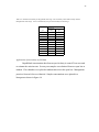
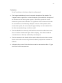
6.6. Histogram of concentrations of ammonia samples taken from open lots. ...............55
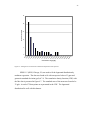
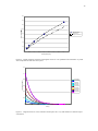
6.7. Cumulative density function for ammonia samples taken from dairy open lot on
July 2004. .............................................................................................................56
7.1. Signal flow of general linear model .........................................................................61
7.2. Output error model ....................................................................................................61
7.3. Laboratory apparatus for determination of system response ...................................63
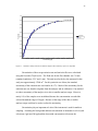
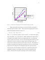
7.4. A plug flow reactor transfer function was found to model the time delay in the
tubing....................................................................................................................67
8.1. Experimental apparatus consisting of mass flow controllers (MFC), flux
chamber, calibration gas, and ammonia analyzers (TEI). ....................................75
8.2. Original Langmuir equation fit and Langmuir kinetics fit .......................................79
8.3. Langmuir kinetics fit ................................................................................................79
x
FIGURE
Page
A.1. LabVIEW program structure showing relationship of programs and
subprograms. ........................................................................................................89
xi
LIST OF TABLES
TABLE
Page
6.1. Uncertainty levels for instrumentation .....................................................................51
6.2. Instrument uncertainty for 20 ppm full scale range .................................................54
7.1. Step responses and transforms to common signal responses ...................................59
7.2. System responses of NH3 analyzer to step inputs of different magnitude...............65
7.3. System responses of H2S analyzer for various inputs ..............................................66
8.1. Chamber time constants and mass adsorbed onto chamber for various
concentrations of ammonia. .................................................................................77
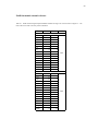
A.1. Details about the digital output FieldPoint modules referring to the valve
references of figure 5.5.........................................................................................90
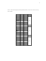
A.2. Details about the digital input and analog FieldPoint modules...............................91
1
CHAPTER I
INTRODUCTION: WHY MEASURE AMMONIA FROM ANIMAL
FEEDING OPERATIONS
An estimated 70% or more of the total ammonia produced in the United States
originates from animal feeding operations (AFOs) (EIIP, 2004). Recently these
operations have been under intense scrutiny for their ammonia production. Ammonia is
known to have a pungent odor and may cause respiratory diseases in both animals and
humans if breathed in large quantities. Particulate matter may form when ammonia
reacts with other compounds in the atmosphere further causing respiratory damage.
Regulators are under increasing pressure to regulate ammonia emissions. However,
ammonia is neither on the list of hazardous air pollutants nor in the national ambient air
standard (U.S. EPA, 2004). The Comprehensive Environmental Response,
Compensation, and Liability Act (CERCLA) requires reporting of ammonia emissions
greater than 100 lbs per day (U.S. House, 2003). Because emission factors have been
developed only for entire operations without regard to management processes, regulators
face a dilemma of regulating an emission without an estimate of how much the operation
is producing or how a management practice may reduce emissions. Since ammonia
production is closely related to management processes, production facilities cannot be
regulated just by their animal production status but must be regulated based on facility
management practices. A science based emission factor must include relationships to
animal type and size, management practices, and climatic effects.
________
This thesis follows the style and format of ASAE Transactions.
2
Several ammonia emission factors have been published. Most emission factors,
however, lack the level of detail needed to use the emission factor for emissions
inventory work (Arogo et al., 2003). These factors are often based upon a nitrogen mass
balance method. Nitrogen inputs and outputs are calculated to determine the nitrogen
loss for a facility. The ammonia production is a function of the nitrogen loss (Phillips et
al., 2000). The mass balance method has many limitations that prevent it from being
used solely for emission factor determination. These limitations include: the inability to
measure the inputs, outputs, and storages accurately; sampling methods and errors
associated with them; and only a small portion of nitrogen is emitted as ammonia
(Phillips et al., 2000). European studies of emissions factors have generally used the
nitrogen mass balance method. Reports by Asman (1992) and Buijsman et al. (1987)
indicate that ammonia emissions in Europe for diary cattle are 39.7 kg/animal-year and
12.7 kg/animal-year respectively. The Compilation of Air Pollution Emission FactorsVolume 1 (AP-42) uses an emissions study performed by the National Acid Precipitation
Assessment Program in 1980 (U.S. EPA, 1985). The emission factor received a poor
rating by EPA for the factor meaning that factor is believed not to be representative of
the population. Arogo, et al. (2003) reported that to determine accurate emission factors,
measurements of swine emission factors should be taken for different weight, building
types, manure treatment systems, and utilization methods.
Currently the only law regarding the emission of ammonia lies in the
Comprehensive Environmental Response, Compensation and Liability Act (CERCLA)
of 1980. The act provides broad authority to respond to release of hazardous substances
that may endanger the public. The act allows the EPA to impose fines on businesses that
emit more than the reportable quantity (RQ) of a pollutant and not report the emission.
The application of the law to animal feeding operation is questioned since the time of
emission is not given and the source is of natural origin. With current emission factors,
dairies may have to report emissions if they have as few as 500 head to have an emission
of over 100 lb/day of ammonia. Since the act is retroactive, fines could be imposed from
the time the act was passed thereby shutting down entire facilities. Currently a handful
3
of lawsuits over ammonia emissions are being debated in court. Each of the lawsuits
cites CERCLA as one reason for suit (US vs. Buckeye Egg Farm, L.P. et al., 2004;
CLEAN vs. Premium Standard Farms, 2001).
If lawsuits set precedent for retroactive regulation of ammonia emissions, one
can only envision the damage to production agriculture. Assuming the emission factor
presented by Asman (1992) was used to determine the threshold for action, the number
of head required to meet the threshold would be approximately 418 hd. Currently 58%
of Texas dairies hold over 500 head (USDA-NASS, 2002). In the US, 41.9% of the
diaries hold over 500 head. Each of these dairies could potentially be affected if
retroactive regulation occurs. Science based process emission factors may allow
operators and regulators to assess the emission to find a proactive solution.
A proper emission factor must be developed for the livestock facilities to be
fairly regulated. Over-regulation causes undo expense to the facility, but underregulation may be detrimental to public health. Regulators must have the necessary
tools to regulate an industry effectively. Regulators may require an industry to develop
and employ best management practices (BMPs) in order to reduce emissions.
The process of determining BMPs involves measuring individual processes
within a facility. By determining process based emission factors, the agricultural
industry may choose management processes that reduce their emissions and therefore
improve public health. Accurate data comparing each management practice must be
presented in a timely manner. In order to obtain data regarding management practices,
efficient use of equipment must be employed.
Process based emission factors are determined by measuring emissions of
individual management processes. For example, an open-lot dairy may have several
management processes such as open lots, milking parlor, solids separation, lagoons, and
compost. Along with the emissions, a nitrogen balance must take place to determine the
relationship of the management change to the overall emissions not just the specific
management process.
4
CHAPTER II
MEASURING TECHNIQUES OF AMMONIA
Ammonia measurement varies by measurement technique and measurement
sensor. Some measurement techniques are better suited for certain types of facilities
than others. This chapter discusses the measurement techniques used to measure
ammonia from AFOs and measurement sensors used to measure ammonia.
Measurement Techniques
Several measurement techniques are available to measure ammonia including:
nitrogen mass balance, plume sampling, flux enclosures, tracer gas, and source
sampling.
Nitrogen Mass Balance
The mass balance method is an indirect method. Physical samples of the source
are analyzed for their nitrogen content and by extension their emission potential. By
tracking the flow of nitrogen throughout the system, the maximum average emission
may be calculated. This method is often used as a check to make sure that the measured
emission flux is within the range bounded by the mass balance method. The mass
balance method may only be used to determine a range of accepted emissions rates due
to the uncertainties associated with measurement of inputs and outputs.
Most of the emission factor development in Europe involved nitrogen mass
balance techniques. Agricultural scientists used years of nutritional research to
determine nitrogen flows in agricultural products. Emissions were determined by
comparing the Nitrogen/Phosphorous ratio across each manure management train
(Asman, 1992).
A mass balance involves estimating the inputs and outputs of nitrogen to the
AFO. Nitrogen may be input in the form of feed and fertilizer. Nitrogen is removed
from the AFO through the sale of agricultural products, volatilization, runoff, and
5
leaching. Only a portion of the total nitrogen volatilized is released as ammonia
(Buijsman et al., 1987).
Nitrogen mass balance has been the preferred method by the US EPA to estimate
emission factors and emissions inventories. Battye et al. (1994) used emission factors
from Asman (1992) to estimate the emissions inventory for agricultural husbandry
operations in the United States. Deficiencies in the knowledgebase were noted from the
study with regard to applicability of European data to developing emission factors for
the United States. Recent updates correlating to measured data may provide a better
estimate of emissions from AFOs (US EPA, 2004).
The advantages of this method are that the method is inexpensive, following a
“cookbook” style for easy baseline regulations, and it lends itself easily as a check for
other methods. The limitations of this method are that it is difficult to characterize all
inputs and outputs and it relies on a large number of critical assumptions. This method
is likely to be used for regulatory purposes.
Plume Sampling
Plume sampling involves measuring upwind and downwind concentrations and
modeling the dispersion of ammonia. The plume sampling method involves sampling
upwind and downwind of the source and back calculating the emission rate using
dispersion modeling. This method may be used with a tower to determine the shapes of
plumes. The sampling method is similar to the particulate sampling methods described
by Sweeten et al. (1998). Dispersion modeling may be based upon Lagrangian or
Gaussian models to develop an emission rate. The solution of the Lagrangian model in
stationary homogeneous turbulence is the Gaussian model (Seinfeld & Pandis, 1998).
Plume sampling is best used for sampling moderate to high emission rates. Low
emission rates may disperse such that the concentration falls below the detection limit of
the sampler. However, plume sampling involves “chasing the plume.” For example, if
the wind drastically changes from North to West, and the sampler is set to sample down
wind of a North wind, the sampler no longer collects an emission from the source in a
6
West wind. The dispersion modeling does not take into account every condition.
Because it is a model, several simplifications are made that may introduce error if the
conditions don’t match the model. The field labor requirements of this method are
reduced dramatically from the flux enclosures method described later in this chapter.
However, the labor requirements are higher in the data processing and analysis stage due
to the requirements of modeling to obtain an emission rate from a downwind
concentration.
The advantages of the plume sampling method and limitations are presented as follows:
Advantages
•
No flush time.
•
Surface moisture conditions not a factor
•
No change to temperature and relative humidity occur.
•
The plume sampling may be used for compounds for which the volatilization is
either liquid or gas controlled.
•
An unlimited number of sensors may be used to measure gas concentrations.
•
Reduced labor in the field.
•
May be used for 24-hour sampling periods
Limitations
•
Plume sampling measures gas emissions indirectly.
•
Wind direction changes result in “chasing the plume.”
•
Low emission rates may have concentrations below the detectable limit of the sensor.
•
Modeling is imperfect.
7
Flux Enclosures
Flux enclosures are small chambers that are placed over the emitting source.
Purified air is introduced at a known rate and the exhaust concentration is measured.
The flux of the source is calculated using:
J=
QC mass
60000A fe
(2.1)
where:
J =emissions flux [µg/m2/s]
Q =flow rate [L/min]
Afe = Area of the footprint of the flux enclosure [m2]
Cmass = Mass concentration [µg/m3]
Two basic types of flux enclosures exist: flux chambers and wind tunnels. The airflow
is not given a particular direction in the flux chamber. Rather, the sweep air is blown
toward the center of the chamber causing eddies to occur. In a wind tunnel, air is blown
across the surface with a given direction.
Sampling points are chosen at random for a given manure management train.
Keinbusch (1986) gives practical guidance on the sampling protocols for the chamber.
The sampling protocol may be adapted to wind tunnels easily.
The flux chamber theory is based on the two-film model (Jiang and Kaye, 1996). The
two film model is often referred to as the phenomenon of volatilization of organic
compounds. This means that the flux chamber may not be used for gases for which the
volatilization process is gas phase controlled. Both hydrogen sulfide and ammonia are
liquid phase controlled (information computed from Linstrom & Mallard, 2005 and
Jiang & Kaye, 1996). Only quiescent surfaces may be sampled with a flux chamber
since the technology is based on the two-film model. The flux chamber cannot be used
for turbulent sources.
8
According to Eklund (1992), the most important operating parameter is the
sweep air flow rate. The optimum sweep air flow rate depends on the design and
operating conditions of the chamber. If the sweep air flow rate is not operating at
optimal conditions, the emission flux may either be underestimated or overestimated. At
high concentrations of the gas being sampled, the flux chamber may actually retard the
emission of the gas from the GLAS. This occurs because the concentration nears the
gas/liquid equilibrium. Because the equilibrium is temperature and humidity dependent,
it cannot be easily determined.
The residence time for the chamber is defined as the time to completely fill the
chamber one time. Eklund (1992) suggests 3 to 4 residence times of flush before
sampling. For example, a 65 L chamber requires approximately 40 minutes of flush at 5
Lpm before sampling can occur. With a single chamber system, this equates to 40
minutes of flush time per sample where the sensors are not being used.
The advantages of the flux chamber method and limitations are presented as
follows:
Advantages
•
Simple inexpensive method to measure gaseous emissions directly.
•
EPA protocol method.
Limitations
•
Different styles and sizes of chambers
•
The flux chamber may only be used for quiescent surfaces. It cannot be used for
turbulent surfaces.
•
Temperature and relative humidity are influenced by solar heating during sampling
•
The flux chamber requires a 40 minute flush time before sampling.
•
The flux chamber may only be used for compounds for which the volatilization
process is liquid controlled (both hydrogen sulfide and ammonia are liquid
controlled).
9
•
Sweep air flow rate must be matched to the chamber type so that emissions are not
overestimated or underestimated.
•
Emission rate may be retarded at high concentrations in the chamber.
•
Emission rate may be increased due to surface disturbance.
•
May only be used during daytime due to worker safety.
Wind tunnels are rectangular structures placed over the GLAS. A fan generates
airflow through the rectangular sample chamber in such a way that the airflow sweeps
across the surface in a linear motion. The wind velocities range from 0.1 to 1.2 m/s
(Schmidt & Bicudo, 2002). This wind speed approximates the ambient wind speed. By
duplicating the ambient wind speeds, one may be able to obtain a more accurate sample.
The inlet air may be filtered for the compound to be measured. Inlet and outlet
concentrations are measured to ascertain that the sampled conditions as close as possible
to ambient conditions. If the wind tunnel is set to filter the air, only the outlet sensor is
needed for the wind tunnel. In this case, the wind tunnel and flux chamber methods may
be compared side-by-side.
Wind tunnel theory is based upon the boundary layer theory (Jiang & Kaye,
1996). Both quiescent and turbulent surfaces may be sampled with a wind tunnel. The
time between samples is reduced from the single flux chamber method because of the
increased flow rate. The wind tunnel is best used for high concentrations of the gas
being sampled. Since the flow rate is much higher for a wind tunnel, more dilution
occurs. At low concentrations, the dilution may cause the concentration to be below the
detection limit of the sampler. The increased flow rate reduces changes in humidity and
temperature within the system. The reduced response time gives the ability to increase
the number of sensors which sample the air. Since no standards exist for the design of
the technology, different size and shape relationships may affect emissions. To avoid
this problem, Schmidt and Bicudo proposed a standard design for a wind tunnel (2002).
The proposed design follows a wind tunnel developed by Lockyer (1984).
The advantages of the wind tunnel method and limitations are presented as follows:
10
Advantages
•
The wind tunnel method measures gaseous emissions directly.
•
Flush time is significantly less with a wind tunnel due to the increased wind speeds.
•
The wind tunnel may be used for quiescent surfaces and turbulent surfaces.
•
Temperature and relative humidity are relatively close to the ambient conditions due
to the rapid air exchange of the system.
•
The wind tunnel may be used for compounds for which the volatilization is either
liquid or gas controlled.
•
An increased number of sensors may be used to measure gas concentrations.
Limitations
•
Air flow rate must be matched to the ambient conditions so that emissions are not
overestimated or underestimated.
•
Low emission rates may have concentrations below the detectable limit of the sensor.
•
Emission rate may be increased due to surface disturbance.
•
No standards for technology.
•
May only be used during daylight at some sites due to worker safety.
Trace Gas
The trace gas method involves releasing a trace gas at a given rate. The
concentrations of ammonia and trace gas are measured downwind. The flux of ammonia
may be calculated using equation 2.2.
11
J NH3
J tracer
=
C NH3
C tracer
(2.2)
where:
J NH3 = Flux of ammonia [µg/m2/s]
J tracer = Flux of trace gas [µg/m2/s]
C NH3 = Concentration of ammonia [µg/m3]
C tracer = Concentration of trace gas [µg/m3]
The trace gas method has been used in the Netherlands to measure the ammonia
emissions from naturally ventilated buildings (Mosquera et al., 2005). Sulfur
hexafluoride (SF6), the trace gas, was injected near the NH3 source. The concentrations
of both SF6 and NH3 were measured near the exhaust of the building. A gas
chromatograph fitted with an electron capture detector (ECD) was used to measure the
SF6 concentration and an AMANDA rotating annular denuder was used to measure the
concentration of NH3 (Scholtens et al., 2004).
The advantages of the trace gas method and limitations are presented as follows:
Advantages
•
May be used in naturally ventilated and mechanically ventilated structures
•
Dispersion modeling not required.
Limitations
•
Trace gas must be emitted near ammonia source
•
Multiple trace gas outlets required for sampling
•
Multiple measurement points required in building
12
Source Sampling
Source sampling involves measuring the flowrate and concentrations of exhaust
points. This method is primarily used for mechanically ventilated structures and
industrial exhaust stacks. Heber et al. (2001) developed a methodology to sample swine
finishing barns. Dust was filtered at each sampling point with the use of a Teflon
membrane filter.
Measurement of airflow is by far the greatest challenge in mechanically
ventilated buildings. The airflow from each fan changes with the static pressure of the
building. The static pressure changes with the number of fans running and the speed of
variable speed fans. Fan performance generally does not match fan curves. The
performance of a fan varies with the loading of dust on the blades. One method of
measuring fan performance is by using the fan assessment numeration system (FANS)
system developed by Simmons et al. (1998). Fans are tested in place with static
pressures ranging from free air to 40 Pa (Gates et al., 2004). With the use of FANS a
new fan curve may be developed for each fan in approximately 30 minutes.
The advantages of the source sampling method and limitations are presented as
follows:
Advantages
•
May be used in mechanically ventilated structures
•
Dispersion modeling not required.
Limitations
•
May not be used in naturally ventilated systems
•
Multiple trace gas outlets required for sampling
•
Multiple measurement points required in building
•
Adsorption on dust not quantified
13
Measurement Sensors
Ammonia emissions may be in the form of ammonia gas and ammonium
particulate. Ammonia emissions may be measured using continuous emission monitors,
wet chemistry, and particulate samplers. Ammonia gas is measured by many different
methods including chemiluminescence, near-infrared light, ultraviolet (UV) light,
electrochemical cells, and wet chemistry.
Ammonia gas measurement
Chemiluminescence involves converting the ammonia to nitric oxide and
measuring the luminescence caused by nitric oxide and ozone reacting in the mixing
chamber (Thermo, 2002a). The chemiluminescence analyzer measures NO, NOx, and
NH3. A stainless steel converter heated to 750ºC is used to convert NH3 to NO. A
molybdenum converter heated to 325°C is used to convert NO2 to NO. The analyzer
multiplexes the three sampling streams to determine the concentration of NH3.
Near -infrared sensors include photo-acoustic and direct optical absorption
sensors. Infrared detectors detect light absorption at 1500 nm wavelength range
(Webber et al., 2001). This wavelength is chosen to reduce interference of water and
carbon dioxide present in the measured gas. The photo acoustic sensor measures
pressure differences caused by ammonia absorbing and desorbing light (Bozoki et al.,
2002). The direct optical absorption sensor measures the adsorption of a selected
ammonia adsorption line (Bozoki et al., 2002).
Ultraviolet instruments based upon differential optical absorption spectroscopy
(UV-DOAS) have been used for open path measurement of ammonia from area sources.
Ammonia absorbs UV light in the 190-230 nm range (Phillips et al., 2001). A Xenon
light source is focused on a receiver placed up to 1000 m away (Myers et al., 2000). A
tunable spectrometer measures the absorption of ammonia. The modulated light source
emits one wavelength that ammonia does not absorb and one wavelength that ammonia
absorbs. The instrument has an interference with components that may attenuate the
light beam (Stevens et al., 1993). These components may be fog, rain, high humidity
14
and dust. Alignment of the transmitter and receiver could be troublesome in field
measurements without an auto alignment mechanism.
Electrochemical cells are small semiconductor circuits that are sensitive to
certain chemicals. The resistance or capacitance changes with concentration. These
sensors have been primarily used as toxic gas monitors. The EC-NH3-100ppm
(Manning Systems Inc, Lexana, KS) has an accuracy of 5% and a repeatability of 2%
full scale (Manning, 2002). Wenger et al. (2005) reported that the Toxi-Ultra ammonia
sensor (Biosystems Inc., Middleton, CT) performed poorly in an agricultural facility.
Hydrogen sulfide reacted with the sensor causing erroneous readings and premature
failure of the sensors.
Wet chemistry involves absorbing ammonia onto an acid solution. The The
ammonia measurement by annular denuder sampling with on-line analysis (AMANDA)
system uses a rotating annular denuder to capture ammonia. Ammonia gas is absorbed
in the acid solution that is pumped through the denuder. Sodium hydroxide is added to
the acid solution and passes across a membrane to deionized water where the
conductivity is measured (Phillips et al., 2001). Classic denuders have used dried oxalic
acid or citrus acid. The acid is washed from the sampler and then titrated with sodium
hydroxide to determine the concentration of ammonia (Leuning et al., 1985).
Particulate Ammonium
The measurement of particulate matter and ammonia in the past has generally
been a disjointed process. This was primarily because of the lack of understanding of
the atmospheric phenomenon in the formation of particulate ammonium.
Particulate matter is generally measured using a gravimetric sampler. This
sampler has an inlet that excludes certain size particles. Currently total suspended
particulate (TSP), PM10, and PM2.5 inlet heads are available. A filter placed after the
inlet captures particles that penetrate the inlet. A vacuum pump is used to pull air
though the inlet head and filter at a measured flow-rate. Gravimetric sampling entails
weighing a filter before and after sampling to determine the weight of particulate
15
collected. The mass of particulate collected on the filter is converted to a concentration
using the time and volumetric flow-rate. Filters must be conditioned in a laboratory
setting for 24 hours prior to weighing to reduce the errors associated with changes in
relative humidity from the field (US EPA, 1998). Since filters must be weighed in a
laboratory setting, volatilization of semi-volatile particles can cause errors in sampling.
Additionally, the filter will cause a change in the equilibrium between the ammonium
particle and the ammonia (Ferm et al., 1988). The change in equilibrium will cause
ammonia to off gas from the particulate as the sample is collected.
Since ammonium particulate is in the form of a semi-volatile particle, it cannot
be measured by gravimetric means. This is because of the ammonia re-volatilizing from
the filter, resulting in an error in the measurement of particulate matter. Without special
care, ammonium particulate contribution to the ambient ammonia concentration is not
taken into account in the measurements.
Several techniques compared by Ferm et al. (1988) may be used to measure both
particulate and gaseous ammonia. One method uses a filter pack for which one filter is
impregnated with a sorbent (oxalic acid) and combined with a pre-filter. The pre-filter is
used to remove the particulate. This method is useful when measuring the total
ammonia concentration (particulate and gas). However, it was shown to overestimate
the ammonia gas concentration. This is because of the equilibrium between the gas and
particulate phases changes with the pressure drop across the pre-filter. Another method
used to measure total ammonia is to use a single filter treated with a sorbent. Only total
ammonia is measured with this method.
Denuder techniques have been used to measure the concentrations of ammonia
gas and ammonium particulate accurately. Denuders take advantage of the fact that the
two phases have different diffusivities in air. The ammonia gas is thus removed from
the particulate ammonium as the air passes along a coated surface under laminar flow.
The particles are collected on a filter. A second denuder is placed after the filter to catch
any ammonia gas that volatilizes off of the filter.
16
Van Putten and Mennen (1995) compared five different techniques for measuring
ammonium aerosol. The five methods included three variations of low volume samplers
as well as a filter pack and annular denuder method. The low volume sampler method
entails sampling as a flow-rate of 1.8 L/min for 24 hours. A denuder filled with active
charcoal was mounted in front of the filter. Several variations of filters were used,
including: standard 8-micron pore size ash-less filter, 8-micron pore size filter
impregnated with citric acid, and a three filter setup. The three filter setup consisted of
three 8-micron pore size filters, with filter one being untreated; filter two treated with
sodium fluoride, and the third impregnated with citric acid. This filter pack used was
similar to the filter pack used by Ferm et al. (1988) except that citric acid was used
instead of oxalic acid. The denuder setup included a 2.5-micron pre-separator, two
denuders coated with sodium carbonate, one denuder coated with citric acid, and a filter
pack with a Teflon filter and citric acid impregnated filter. Ammonium sulfate aerosols
were generated and mixed with ammonia gas. The particle size distribution of the
aerosol was determined with a scanning mobility particle sizer (TSI SMPS model 3934).
Van Putten and Mennon (1995) found that the low flow samplers in each case reported
concentrations lower than the annular denuder. One of the main problems with the
measurement techniques using a denuder is the response time. The denuder often
requires 8 to 24 hours of ammonia flux before it can be analyzed. This poses a problem
when trying to analyze contributions from an area source. Often the wind direction will
change significantly throughout the day resulting in capture of gas only part of the time.
17
CHAPTER III
CHALLENGES FACING AMMONIA MEASUREMENT FROM
AGRICULTURAL FEEDING OPERATIONS
Measuring ammonia from AFOs is a difficult and expensive task to perform.
Many factors affect ammonia emissions ranging from management decisions to climate
conditions. Many challenges exist when measuring ammonia from agricultural feeding
operations.
Facilities from animal feeding operations may be classified into two types: barns
and open areas. An AFO usually contains multiple facilities throughout its operation.
Design of such facilities varies depending on the contractor used. However, guidelines
and standards exist for the design and use of specified types of facilities. Guidelines are
available from Midwest Plan Services, CIGR, ASHRAE, and ASABE.
Factors Affecting Ammonia Production
Many factors affect ammonia production from animal feeding operations.
Understanding how ammonia is emitted and the factors affecting the emissions provides
an important strategy for reducing emissions. To understand how ammonia is produced,
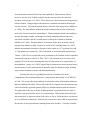
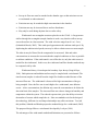
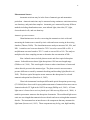
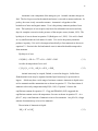
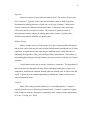
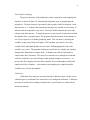
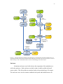
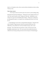
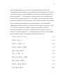
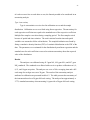
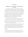
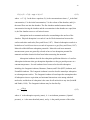
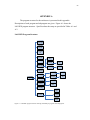
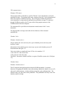
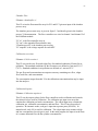
the processes of waste breakdown must be examined. Figure 3.1 details the breakdown
of animal waste.
18
Animal
Protein
Plant Protein
Animal Waste
Feed Waste
(Organic N)
Fecal Matter
(Organic N)
Dead
Bacteria
(Organic N)
Urine
(Urea)
Denitrification
[NO2-]
Uric Acid
Decomposition
Mineralization
(Bacterial Oxidation)
And
Bacterial Decompostion
[NH3]G
[NH3]L
Hydrolysis of Urea
Mineralization
(Bacterial Oxidation)
And
Bacterial Decompostion
[NO]
[N2O]
[NH4+]L
Volatilization
[N2]
Nitrification
NO, N2O
[NO2-]
[NO3-]
Figure 3.1. Breakdown of animal waste. The breakdown of animal waste is a natural process of the nitrogen cycle.
Ammonia, nitrogen oxide, nitrous oxide, nitrogen, and nitrogen dioxide are gaseous products of the breakdown
process (USDA, 1992; Takaya et al., 2003; Robertson et al., 1988).
19
Ammonia is one component of the nitrogen cycle. Animals consume nitrogen as
feed. The feed is processed in the animals and waste is excreted as manure and urine. In
poultry, the waste is only excreted as manure. Ammonia is a byproduct of the
breakdown of urine and organic matter. Urea is the primary ammonia producer from
urine. The hydrolysis of urea requires only hours for substantial conversion and only
days for complete conversion in the presence of the enzyme urease (Asman, 1992). The
hydrolysis of urea is shown in equation 3.1(Rodriguez et al., 2005). Uric acid is found
in very small amounts in fecal matter for cattle. Uric acid is the primary ammonia
producer in poultry. Uric acid is decomposed aerobically to form ammonia as shown in
equation 3.2. Protein in the feed and animal waste is mineralized and decomposed to
form ammonia.
Hydrolysis of urea:
CO(NH 2 )2 + 3H 2 O ⎯Urease
⎯⎯→ CO 2 + 2 NH 4+ + 2OH −
(3.1)
Aerobic decomposition of uric acid:
C 5 H 4 O 3 N 4 + 1.5O 2 + 4H 2 O → 5CO 2 + 4 NH 3
(3.2)
Animal waste may be scraped, flushed, or stored in deep pits. Solids from
flushed animal waste may be separated and the liquid waste may be processed in a
lagoon. Solids may have a wide range of moisture contents. Ammonia in liquid exists
as free ammonia and the ammonium ion as shown in equation 3.3. The dissociation of
ammonia is driven by temperature and pH (Ni, 1999). Equation 3.4 shows the
equilibrium constant for equation 3.3. Clegg and Whitfield (1995) suggested the
equilibrium constant varies with temperature for water as shown in equation 3.5. At a
pH of 7, only a small amount of ammonia exists as free ammonia. At a pH of 8, a larger
amount of ammonia may exist as free ammonia.
Dissociation of Ammonia in liquid:
NH 3 + H + ↔ NH +4
(3.3)
20
10−pH [NH3 ]L
Kd =
NH4+ L
]
(3.4)
2729.33 ⎞
⎛
pK d = ⎜ 0.090387 +
⎟
T ⎠
⎝
(3.5)
[
where:
pK d = − log10 K d
(3.6)
K d = Equilibrium constant
[NH 3 ]L
= Concentration in liquid phase of free ammonia
[NH ]
= Concentration in liquid phase of ammonium ions
+
4 L
T = Temperature [K]
To understand volatilization of ammonia, the two film theory developed by Lewis
and Whitman (1924) may be employed. In the two film theory, three steps of ammonia
mass transfer occur: the convective mass transfer from the surface of the gas film to the
free air stream, the diffusion across the boundary layer, and diffusion inside the bulk
manure. An overall mass transfer coefficient is often used to describe the entire two film
theory. Arogo et al. (1999) defined the overall mass transfer coefficient to be a function
of air viscosity, diffusivity in air, air velocity, liquid temperature, air temperature, and a
characteristic length.
Nitrification is a process where the ammonium ion is oxidized by autotrophic and
heterotrophic bacteria to form nitrites and nitrates. Nitrification requires oxygen to form
nitrites. The byproducts of autotrophic bacteria are different from the byproducts of
heterotrophic bacteria. Autotrophic bacteria exist in aerobic conditions, while
heterotrophic bacteria exist in both aerobic and anaerobic conditions. The role of
heterotrophic bacteria in the nitrogen cycle is unknown (Robertson et al., 1988).
21
Denitrification is the sequential reduction of nitrates and nitrites to nitrogen gas.
Denitrification may take place aerobically or anaerobically (Robertson et al., 1988). One
of the byproducts of the denitrification process is nitrous oxide (Takaya et al., 2003).
Measuring Ammonia in Barns
Barns in AFOs provide a containment structure with necessary shelter from
nature’s elements. Barns may be classified into naturally ventilated and mechanically
ventilated facilities. Ventilation in barns provides multiple functions, including removal
of gases, such as ammonia, from the barn while providing clean, fresh air to the animals.
Temperature in the barns is regulated in part by changing the ventilation rate of air
through the barn. Poultry and pork are often housed in barns. Dairy cattle may be
housed in barns or open lots. The frequency of removal of manure from barns varies
from one operator to another.
Naturally Ventilated Barns
A naturally ventilated barn is a barn for which the ventilation is driven by nonmechanical forces of wind and buoyancy (Bartali and Wheaton, 1999). In a naturally
ventilated barn, the temperature and ventilation rate are controlled by the opening and
closing of openings to the building. The exhaust often flows through a ridge opening
that spans the top of the roof.
Dairy freestall barns in the southern United States are a type of naturally
ventilated barn. Freestall barns are generally more open than other naturally ventilated
barns where the temperature needs to be controlled. A concrete floor may be scraped or
flushed.
Naturally ventilated barns are particularly difficult to measure because the
ventilation rate is often unknown and very difficult to measure. One method of sampling
is upwind and downwind sampling. Multiple houses and waste handling are often built
for the operation. It is difficult to compare emissions from one house to another.
22
Mechanically Ventilated Barns
A mechanically ventilated barn is a facility for which the ventilation is driven by
fans. In a mechanically ventilated barn, fans may be placed either on one end of the barn
or spaced along the sides of a barn. Fans are turned on and off to control the temperature
and ventilation rate of the barn. In some hog barns, manure from the pigs drops into a
pit under the barn. Several fans are used to draw air across the manure to reduce the
concentrations of gases inside the building.
Mechanically ventilated buildings pose several challenges for the measurement
of ammonia. Airflow through these building varies seasonally and temporally. For
example, the recommended airflow for a layer facility is 0.85 m3/h/bird (0.5 cfm/bird) in
cold weather and 6.8 m3/h/bird (4 cfm/bird) in warm weather (MWPS, 1983 ). A typical
25,000 bird broiler house may have ten 1.2 m (48 in) diameter fans. A typical 100,000
bird layer house may have 50 0.9 m (36 in) diameter fans. Fans are typically turned on
and off to regulate the airflow. Some newer facilities have adopted variable speed fans.
When sampling mechanically ventilated buildings, selection of the sampled
exhaust fans is random (Heber et al., 2001). It is expected that the concentrations
leaving the exhaust may not be uniform from one exhaust to another. This depends on
the configuration of the house and whether animals were able to bunch in a particular
area.
Measuring Ammonia in Open Areas
Open areas may be classified as open lots, manure storage, or compost.
Emissions from open lots may be measured by nitrogen mass balance,
upwind/downwind concentration measurements, flux enclosure, or trace gas methods.
Emissions from open areas are likely to be heterogeneous since animal location and
manure accumulation will most likely be heterogeneous.
23
Open lots
Open lots consist of pens in which animals are held. The surface of most open
lots is soil based. Typically feeder cattle and some dairy cattle are held in open lots.
Recommended stocking densities of open lots vary by type of animal. Cattle tend to
locate in some areas within the lot more than others. Cattle may create craters that
collect urine and feces on the pen surface. The surfaces of open lots tend to be
heterogeneous in nature ranging in loading and moisture content. Operators have
different scrape and fill schedules for open lot pens.
Manure Storage
Manure storage involves solids storage, slurry pits, retention ponds, and lagoons.
Much of the solids waste may be removed from flushed manure through the use of solids
separation. Scraped manure from open lot pens and barns may be piled until time to
land-apply the byproduct. Slurry pits hold high solids content manure. This manure is
often land applied using special liquid manure injection systems or with the use of liquid
spreaders.
Liquid manure stores may be aerobic, facultative, or anerobic. The byproducts of
these bioreactors are dependent on many factors including loading rates, oxygen, pH,
temperature, and bacterial condition. Runoff ponds are holding areas for flush water and
runoff. Lagoons provide treatment depending on loading rate, manure characteristics,
and environmental factors.
Compost
Some AFOs compost manure and hay for a value added product. Compost is
typically placed in rows so that it may be turned easily. Compost is turned on a regular
basis to improve aeration. During the composting period, compost reaches temperatures
of 50-60 °C (Liang et al., 2004).
24
CHAPTER IV
RESEARCH OBJECTIVES
The goal of this research is to provide the ability to measure emissions of
ammonia from AFOs. By providing the ability to measure ammonia effectively, BMPs
may be developed to aid operators of AFOs to reduce emissions. Two primary
objectives were established to meet the goal of this research:
1. Develop a process based measurement system for analyzing and evaluating
BMPs relating to fugitive ammonia emissions from AFOs. The system
presented will improve current sampling methods through improved data
management, increased sampling rate, and a more user-friendly interface.
2. Evaluate system performance for the given operating conditions to determine
if system will meet acceptable criteria. The performance of the system will
be tested for uncertainty, system response, and adsorption. The uncertainty
of the system is expected to be less than 20% for the given operating
parameter. An uncertainty budget of the instrument will be developed to
determine system uncertainty. The system response of the instrument is
expected to allow for the measurement of ammonia. System response will be
modeled to determine the limitations of the system. Adsorption on chamber
surfaces is not expected to significantly affect the measurement of
concentrations in the chamber. The adsorption kinetics will be tested for the
chamber to determine the significance.
25
CHAPTER V
DEVELOPMENT OF A PROCESS BASED MEASUREMENT
SYSTEM
The Center for Agricultural Air Quality Engineering and Science (CAAQES)
uses several methods to measure ammonia and hydrogen sulfide from ground level area
sources (GLAS). These measurements are primarily taken from AFOs. Generally,
CAAQES has used a method detailed by Kienbusch (1986) using emission isolation flux
chambers to measure ammonia and hydrogen sulfide emissions. CAAQES had acquired
two 17C (Thermo Inc. Franklin, MA) ammonia analyzers, one 45C hydrogen sulfide
analyzer, and one 450C hydrogen sulfide analyzer, and required enhanced efficiency of
field sampling because of increasing costs. Every field process step was examined to
reduce the time of sampling. This study focused on data management, time
management, and protocol development. The goal of this work was to present the
design a multiplexer system for CAAQES to measure ammonia and hydrogen sulfide
more efficiently during field sampling.
Background
The flux chamber method is based upon the two-film model (Jiang & Kaye,
1996). The two film model relates the emission flux of a gas to the concentration of the
gas in the liquid using Henry’s Law and diffusion. Several factors affect Henry’s law
and diffusivity, including concentration gradient, temperature, and pressure. These
factors are often not addressed by those using the flux chambers.
Humidity can largely affect measured emissions since water can combine with
volatilized ammonia. Care must be taken to not increase the temperature of the air in the
chamber and sequentially reduce the temperature in the lines since this could result in
condensation. Condensation can adversely affect the thermal mass flowmeters as well as
the analyzers. The ammonia and hydrogen analyzers are capable of handing water vapor
but not liquid water.
26
While ammonia is of high concern at CAAQES, hydrogen sulfide is also a
concern. An analyzer bank consists of one ammonia analyzer and one hydrogen sulfide
analyzer. The original system and new system were designed such that both analyzers in
the analyzer bank could be used simultaneously.
Original System
Originally, only one flux chamber was used by CAAQES to sample emissions
from AFOs. The sampling process took approximately 1 hour to sample plus time to
move the flux chamber from one location to another. The flux chamber required 15
minutes to move when sampling a lagoon and approximately 5 minutes to move on dry
surfaces. The total time required to obtain a sample was conservatively estimated to be
1 hour 15 minutes.
LabVIEW 5.1 (National Instruments, Austin, TX) was the programming
language of choice for the original setup. Three programs were required to obtain data
and control the gas flow to and from the chamber. The first program controlled the flow
rates using a mass flow controller (MFC series, Aalborg Instruments, Orangeburg, NY)
via a DAQCard (AI-16-XE-50, National Instruments, Austin, TX) coupled with two
digital to analog converters (Maxim 544, Dallas Semiconductor, Sunnyvale, CA). The
second program logged data from the analog outputs of the analyzers every five seconds.
Temperature data from the ambient air, flux chamber, and source were also recorded
every five seconds. The five second data proved to be cumbersome to analyze and the
one minute data was determined to be sufficient for estimating gaseous emissions. The
third program provided concentration data from the analyzers via the RS-232 serial port.
The digital and analog data were each logged into a file.
Calibration of the analyzers involved attaching a gas cylinder of known
concentration to the system. The calibrated gas was mixed with zero air to reduce the
concentration of the gas as needed. A static mixer (1/2-80-PFA-12-2, Koflo
Corporation, Cary, IL) was used to mix the gas thoroughly. The calibration was
performed according to manufacturer’s recommendations.
27
As data collection progressed, a few shortcomings with the original setup became
apparent. First, the single chamber only allowed the sensor to be used less than half of
the time. This limited the total number of samples to approximately 35 for a 4 day
sampling period when sampling 13 hours per day. Data management was also a
problem. Data was lost and was difficult to manage because of the multiple program
structure. The non-integrated program structure was also difficult for the user to
navigate.
The method of flux chamber sampling is described in detail by Kienbusch (1986)
in Measurement of Gaseous Emission Rates from Land Surfaces Using Isolation Flux
Chamber. The CAAQES protocol follows this method. Upon arriving at the AFO, the
site is divided into various manure handling, storage, treatment, and animal confinement
units. This identifies areas emitting the measured gases. For example, a dairy in Central
Texas may be divided into freestall, open lot, solids separation, lagoon, and composting
areas. Each of these units is further divided into random samples. The number of
samples depends on the total surface area and consistency of the area. Statistical
analysis was used to determine the number of samples required for each unit.
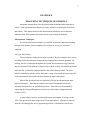
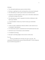
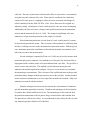
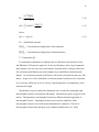
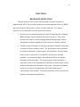
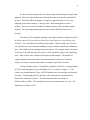
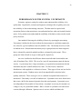
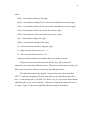
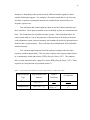
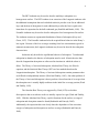
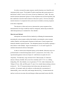
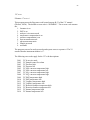
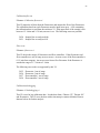
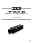
The flux chamber used by CAAQES has a diameter of 0.495 m, a cylinder height
of 0.24 m, and hemispherical top with height of 0.17 m as shown in figure 5.1. The
cylinder was manufactured of 10 ga. AISI 304 stainless steel for durability and chemical
resistance. The hemispherical top, inlet tube, and outlet tube were purchased from
Odotech Inc. (Montreal, Quebec). The inlet and outlet tubes were made of
PerFluoroAlkoxy (PFA). The hemispherical dome was manufactured of acrylic. The
chamber has a volume of 65 L.
28
OUTLET
ACRYLIC TOP
INLET
0.17
SWEEP AIR TUBE
0.24
STAINLESS
STEEL
SKIRT
0.495
Figure 5.1. Schematic of the flux sampling chamber used by CAAQES.
The sampling process begins when the chamber is placed on the GLAS. A flow
rate of 7 L/min (21°C, 1atm) of zero air from a gas cylinder or zero air generator (73712A, AADCO, Village of Cleves, OH) is pumped into the chamber as a sweep air. Zero
air is air that has been purified to remove pollutant gases. Two to four liters per minute
(21°C, 1 atm) are drawn from the chamber and the flow is split into one hydrogen sulfide
analyzer and one ammonia analyzer. The chamber is vented to the atmosphere so that
the remaining gas exits the chamber. The chamber is flushed for thirty minutes followed
by thirty minutes of sampling.
Goals
A new integrated system was proposed for which analyzer downtime was almost
zero. The new system multiplexed three chambers for each set of ammonia and
hydrogen sulfide analyzers. This allowed the analyzers to be used continuously
throughout the sampling trip. The system allowed collection of over 80 samples during
29
a four day sampling period from a single analyzer at an average rate of 1.33 samples per
hour including system setup and takedown each day. Because of the increased amount
of data received from the analyzers, a good data management system was essential.
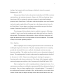
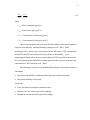
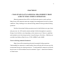
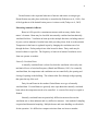
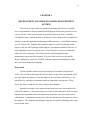
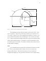
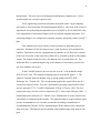
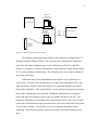
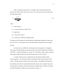
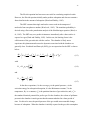
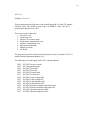
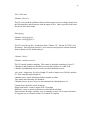
The multiplexer system allowed multiple receptors to be sampled using a single
analyzer. Three chambers could be placed on an emitting source and samples taken
sequentially. Figure 5.2 shows a diagram of the multiplexed chamber setup placed in a
field setting.
1
6
9
10
Ready
Flush
7
12
3
2
8
11
Sample
Mobile
Lab
4
5
Figure 5.2. Multiplexed chamber setup. The mobile lab is placed near the center of the sampling area. Three flux
chambers are placed in random locations within a sample area grid. Grid areas are chosen at random with respect to
time. Flux chambers are sampled sequentially by the analyzer with the use of the multiplexer.
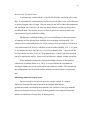
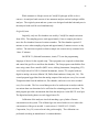
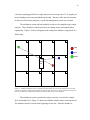
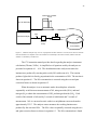
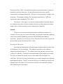
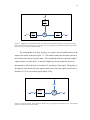
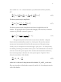
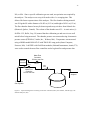
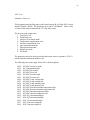
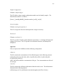
The multiplexer system controls three major processes: zero air flow, sample
flow, and chamber lift. Figure 5.3 shows one chamber with the major control processes.
The chamber must be lowered at the beginning of each test. After the chamber is
30
lowered, the zero air flow begins and remains until the end of the sample. The chamber
is flushed for 30 minutes followed by a 30 minute sample. The chamber is flushed to
remove effects due to the response time of the chamber. The chamber is lifted at the end
of the sample so that it may be relocated for the next sample.
Zero Air
Generator
Ze
Air
Compressor
Sam
ro
A ir
ple
Multiplexer
C
m
ha
Analyzer
ift
rL
be
Vent
Flux Chamber
Figure 5.3. Multiplexer control of chamber. The multiplexer controls the chamber lift, sample flow, and zero air
flow. An air compressor supplies air for the chamber lift. A zero air generator provides zero air for the chamber.
The multiplexer control included a series of solenoid valves (Gold Ring Series
20, Parker Hannifin Corp., Madison, MS) that open and close to calibrate, run and flush
the system. These valves were controlled via Fieldpoint modules (National Instruments,
Austin, TX). LabVIEW 7.1 software was used as the control interface for the Fieldpoint
modules. Mass flow controllers (MFC series, Aalborg Instruments, Orangeburg, NY)
were used to adjust the zero air flow rate entering the chamber. Needle valves (#0639380, Cole-Parmer, Chicago, IL) were used with mass flow meters (MFM series, Aalborg
Instruments, Orangeburg, NY) to adjust the flow of air to be analyzed.
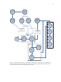
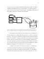
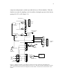
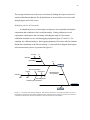
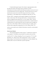
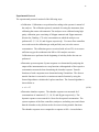
A schematic of the control system is presented in Figure 5.4. Chambers were
controlled by a pneumatic lift mechanism to lower the individual chamber at the
beginning of the test and raise the chamber at the end of the test. All of the chambers
were initially in the upward position with S18, S20, and S22 open (figure 5.4). An air
31
compressor and pneumatic cylinders provided the force to lift the chambers. When the
chamber was ready for sampling, it was lowered by releasing the pressure in the lines by
opening S19, S21, or S23 (figure 5.4).
NC Solenoid Valve
S1
Mass Flow Controller, 15 L/min
S2
MFC1
Zero air to
Chamber
S3
Zero Air Generator
S4
MFC2
S5
Mass Flow Controller, 15 L/min
To Additional Analyzers
for Calibration
S6
S7
Pressure Regulator
MFC3
Static Mixing
Element
S17
Mass Flow Controller, 5 L/min
Calibration
Gas
S18
S19
S20
Pressure Regulator
Backflow Valve
S8
S9
Dryer/Water Separator
S21
NO Solenoid Valve
S10
MFM1
To Chamber Lift
System
S22
S16 Mass Flowmeter
Vacuum Pump
S23
S11
Air Compressor
FV1
Sample
Flow
From
Chamber
S12
FV2
S13
FV3
S14
Adjustable Flow Valve, 2 L/min
S15
Mass Flowmeter
Analyzer
MFM2
Teflon Vacuum Pump
Figure 5.4. Multiplexer schematic. The multiplexer controls zero air flow, sample flow, and pneumatic lift.
Additional multiplexers may be calibrated with the use of valve S17. Mass flow controllers automatically control the
flow. The mass flow meters measure the sample flow from the chamber. Solenoid valves control the flow to each
chamber.
32
Only two of the three chambers were used at any given time. Two mass flow
controllers (MFC1& MFC2, figure 5.4) were used to control the zero air flow rate into
the chambers. Manifolds and six solenoid valves (S1-S6, figure 5.4) were used to
distribute the zero air to the respective flux chambers.
Air from the chambers was drawn through Teflon PFA tubing into the enclosure
where it was metered using a needle control valve (FV1-FV3, figure 5.4). Six solenoid
valves (S9-S14, figure 5.4) controlled the path of flow. The valves were place in the off
position when the chamber was inactive. Two flow paths may be chosen if the chamber
was active depending whether the chamber was in flush mode or was in sample mode.
A standard duty vacuum pump (117CAB18, Thomas Industries, Louisville, KY)
maintained the flow during flushing (first 30 minutes). A second vacuum pump
(N810FTP, KNF Neuberger, Inc., Trenton, NJ) drew the flow to the analyzer during the
sampling period. A mass flow meter (MFM1 & MFM2, figure 5.4) indicated the flow
rate from the chamber.
A gas dilution system was incorporated into the multiplexer for calibration of the
analyzers. Flow of regulated calibration gas was controlled with a mass flow controller
(MFC3, figure 5.4). Zero air flow was controlled by MFC2 and S7. The zero air and
calibration gas are mixed using a static mixing element (1/2-80-PFA-12-2, Koflo
Corporation, Cary, IL). Since only one calibration system is required for both analyzer
banks, a solenoid valve (S17) is available for the calibration of the second analyzer.
Multiplexer Programming
The multiplexer program may be divided into several areas. The subprograms
are designed to be modular so that the measurement system may be used with other
sampling methods. Programming of the multiplexer system is performed in LabVIEW
7.1 (National Instruments, Austin, TX). Details of the subprograms are presented in
appendix A.
33
Flux Chamber Sampling
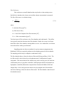
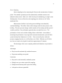
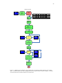
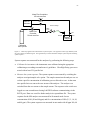
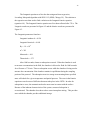
The process structure of the multiplexer used in conjunction with sampling flux
chambers is shown in figure 5.5 illustrating the important steps in programming the
multiplexer. The data structure is presented in the top right of the flow diagram. In the
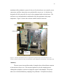
data structure, a “1” indicates the component referring to the variable is active and a “0”
indicates that the component is not active. The bold variables indicate the sum of the
column in the data structure. To begin the process, a user pressed a button that activated
the chamber after it was positioned. The program checked the status of the chamber to
see if it was in queue or in flushing/sampling mode. This was done by checking the
variables: ready (sum), flush, and sample. If all variables were inactive, the ready
variable for the individual chamber was activated. Nothing happened if any of the
variables were active. The program continuously checked to see whether any chamber
changed from flush mode to sample mode. A chamber moved from flush mode to
sample mode after 30 minutes. The mass flow controllers were multiplexed such that
each flow controller was used at all times when multiple chambers were active. To
preserve the flow integrity, the same flow controller was used throughout a flush and
sample period for a chamber. At 60 minutes, the sampling was completed and the
variables were reset for the chamber.
Calibration
Calibration of the analyzers was performed by a dilution system. In this system
calibrated gases were diluted to the required level for multipoint calibration. Calibration
procedure was followed according to manufacturer’s specifications as outlined in the
instruction manuals.
34
Chamber Processes
Input:
Start
Chamber
Check
Ready=0
Flush =0
Sample =0
Chamber
Ready
(Ready = 1)
No
Check
Flush = 0
Chamber Flush Sample Ready mfc1 mfc2 T(chamber)
1
1
0
0
0
1
8:30
2
0
1
0
1
0
8:00
3
0
0
0
0
0
sum
1
1
0
1
1
Yes
Write
Flush =1,
Ready =0
Choose MFC
If MFC 1 = 0
Write mfc 1 = 1
Else write mfc 2 = 1
Write
Time = {current time}
Input data
Flush
Output
Process
Information
Yes
Check Time
(Flush)
{current time}
<Time+30 min
No
Write
Flush=0
Sample =1
Input Data
Sample
Check Time
(Sample)
{current time}
<time +60 min
Output
Process
Information
Yes
Output
Log and
Save Data
No
Write
Sample = 0
mfc 1 =0
mfc 2 =0
End
Figure 5.5. Multiplexer process diagram. Only a chamber that is not in flush or sample mode may enter an empty
queue. A chamber in flush mode enters sampling mode when the sampled chamber completes sampling. A chamber
enters flush mode after the flushed chamber enters sample mode.
35
Error Checking
Checking for errors is an important part of any complex system. The program
enabled the system to check for flow rate errors and alerted the user of the error as it
occurred. The error checking had several levels of errors. If an error was severe
enough, the chamber was stopped and allowed to begin again. Before each sampling
period, the sample lines were flushed to ensure that no condensation remained in the line
from the previous sample. This was one method to reduce the chance of damaging a
mass flow meter or mass flow controller.
Data Acquisition
Data acquisition is an important function of the instrumentation. Data from the
analyzers was logged as well as temperatures from the chambers. Temperatures were
logged using data loggers (HOBO H08-008-04 with TMC6-HC temperature probes,
Onset, Pocasset, MA) that were placed on each chamber. The temperature inside the
chamber, outside the chamber, and from the source were measured each minute.
Relative humidity was logged on two of the six chambers. Data was downloaded from
the data loggers every 24 hours to a computer using serial digital interface and BoxCar
Pro software (Onset, Pocasset, MA). Temperature data was exported to a tab delimited
text file for input in a spreadsheet or database. One minute concentration averages were
output from the analyzers using a serial digital interface through LabVIEW. Flowmeter
data and concentration data were saved to a comma delimited text file.
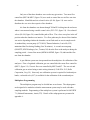
User Interface
A user interface was provided for the user. The user interface consisted of a 5.7”
touchscreen panel (TPC-642SE-CE, Advantech, Cincinnati, OH), three momentary on
selector switches and three momentary on push button switches. The touchscreen panel
allowed users to view system status including concentrations, chamber status, system
errors, flowrates. Users input the sampling source by using the touchscreen. The
selector switches were used to activate the particular chamber. An indicator light in the
switch indicated whether the chamber was active. Once the chamber was active, a push
36
button was pressed to place the chamber in queue. Figure 5.6 shows the user interface of
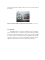
the multiplexer.
Figure 5.6. User interface of the multiplexer. The interface consists of: selector switches to activate each chamber,
push button switches to place a chamber in queue, and a touchscreen to display pertinent data.
Data Management
Data management plays a key role in the sampling trips. Data flow through the
system is presented in figure 5.7. Temperature was logged by the data loggers (HOBO
H08-008-04 with TMC6-HC temperature probes, Onset, Pocasset, MA) and downloaded
to a computer. Flowmeter and concentration data were logged and saved to a flash data
card located in the touch screen. The data was downloaded to a computer by using an
USB link to a computer and ActiveSync software (Microsoft, Redmond, WA).
37
PC Computer
With
Boxcar Pro
Concentration
Data
Launch
Dataloggers
Temperature
& RH Data
Thermo
17C & 45C
HOBO
Dataloggers
User
Switched
Inputs
Download
Dataloggers
PC Computer
With
Boxcar Pro
Serial
Communications
Flowmeter
Data
NI
FieldPoint
Ethernet
FTP
Advantech
Touchscreen
User Inputs
Flashcard
Storage
Save &
Retrieve
Data
PC Computer
with
Database
Chamber
Indicator
Lights
Data Display
Download Data in
Spreadsheet Format
Via USB
PC Computer
With
ActiveSync
Conversion of
Files and
Data Analysis
Additional
Inputs to
Database
Flowmeter
Control
Analyzed
Data
Figure 5.7. Data flow through the sampling system. Dataloggers record temperature and relative humidity data. The
NI FieldPoint modules collect flowrate and concentration data and sent the data to the touchscreen where it is saved on
flashcard storage. Data is downloaded from the touchscreen and dataloggers for further analysis.
Enclosure
Aluminum enclosures were built to house the components of the multiplexer as
well as the analyzers. Each enclosure was built so that it could be pulled with an all
terrain vehicle. This allowed the two analyzer banks to be positioned up to 50 m apart.
The enclosures were sized to contain a standard rack system and included an area for
38
attachment of the multiplexer system. In the rear of each enclosure, user controls, power
connections, and flow connections were positioned for easy access. A side door was
designed to be fully removable for access to the equipment inside each enclosure. The
enclosures were insulated and air conditioned to keep the equipment at the proper
temperature. Figure 5.8 shows the enclosure with the side door removed.
Cooling System
Multiplexer
Analyzer Bank
Power
Distribution
.
Figure 5.8. Enclosure with side door removed. Components are placed for easy access in the enclosure. Each
enclosure contains an analyzer test bank, power distribution system, multiplexer with flowmeters, and cooling system.
Summary
The new system increased the number of samples taken, allowed better retention
of data and was easier to use. This increased productivity for the sampling period.
Although the multiplexer system was designed to operate with chambers, it may have
other uses in field and laboratory sampling of air pollutants. CAAQES can currently
39
obtain over 90 samples per day with two analyzer banks and multiplexers when working
24 hours per day.
Future Improvements
Several improvements can still be made to the enclosure system including tubing
management and replacement dataloggers. Tubing may become entangled in the feet of
cattle in the open lots and free stalls, resulting in a broken line. Additionally several
wrenches are required to attach and detach the chambers. Tubing may be managed by
providing quick disconnects, covering the lines, and limiting the amount of excess line
run out.
Current dataloggers do not allow for integrated data management. Temperature and
relative humidity is logged separately from the concentration and flowrate data.
Additionally, some problems have been found with data integrity of the current
dataloggers. This problem has been identified as a faulty connection between the
datalogger and temperature sensor. The sensor may become partially disconnected
without the user knowing resulting in the entire data set being lost for that datalogger.
40
CHAPTER VI
PERFORMANCE OF THE SYSTEM: UNCERTAINTY
Scientists, engineers, and policy makers must understand the reliability of air
quality data. In particular, scientists and engineers working in the air quality sector use
the reliability of data in determining emissions. The data must be reported with
uncertainty limits so that practitioners can understand and use what was learned from the
study. Policy makers must understand the credibility of the data in order to make sound
policy decisions.
One method of showing the reliability of data is by reporting the uncertainty.
Uncertainty is defined as the interval about the measurement or result that contains the
true value for a given confidence interval (ASME, 1998). Uncertainty arises as a result
of random errors. Measurement uncertainty may be grouped into two main categories:
those evaluated by statistical methods and those evaluated by other means. These
groups are often referred to as type A and type B, respectively.
An error is defined as the difference between an individual result and the true
value (Eurachem/Citac, 2000). The error for a specific measurement cannot be known
exactly. A system may have a large uncertainty, yet a particular measurement with the
instrument may have a small random error value. For this reason, a statistical
distribution is often applied to a collection of errors. Three types of error are involved in
measurement systems. Random errors arise from unpredictable variations in the
quantity measured. These errors give rise to variations in repeated observations of a
measurand. Uncertainty is a result of random error. Systematic errors arise from factors
that create a shift in the measured quantity from the actual quantity. Systematic errors
are independent of the number of observations. Systematic errors may be constant over
a range or vary in a predictable manner. Bias is a result of systematic error and can be
corrected through calibration. Spurious error is an error which invalidates the
41
measurement. This error arises from instrument malfunction or human error. Lost or
invalid samples are a result of spurious error.
Every engineering system has uncertainty associated with it. In gas sampling,
uncertainty is often associated with instrumentation and flow. One focus at the Center of
Agricultural Air Quality Engineering and Science (CAAQES) at Texas A&M University
is the maintenance of uncertainty budget for all air pollution sampling equipment. The
uncertainty budget is one component in a quality assurance and quality control (QA/QC)
plan.
Flux chambers have been used by several researchers to determine gaseous
emissions. Kienbusch (1986) developed a user’s guide for the use of an isolation flux
chamber. Purified air (zero-air) is pumped into the chamber at a set flow rate by means
of the zero-air stream. At the same time, polluted air is extracted by means of the sample
stream. The sample stream flow rate is less than the zero-air stream flow rate. The
differential flow is vented through the top of the chamber to insure that a positive flow
out of the chamber vent occurs.
In the CAAQES protocol, the zero-air flow is set at 7 sL/min and the sample
flow at 2 to 4 L/min. The simplified sampling setup is presented in figure 6.1. The
sample is extracted from the chamber using a vacuum pump (N810FTP, KNF
Neuberger, Inc., Trenton, NJ). The vacuum pump supplies the required flow rate of 2
L/min to the analyzer sensor. Zero-air is generated by purifying compressed air with a
zero-air generator (737-12, AADCO Instruments, Village of Cleaves, OH). The air is
compressed using a oil-less scroll air compressor (SF-2, Atlas-Copco, Holyoke, MA). A
chemiluminescence analyzer (17C, Thermo Corp., Franklin MA) is used to measure the
concentration of ammonia in the chamber. The ammonia analyzer requires that the input
pressure be atmospheric so a vent tube was attached according to manufacturer’s
recommendations (Thermo, 2002a). Standard ranges for the analyzer have a maximum
span of 20 ppm. The analyzer may be operated with extended ranges with spans to 100
ppm.
42
Mass Flow Controller
7L/min
Zero Air Generator
Vent
Ammonia Analyzer
Vent
Needle valve 2L/min
Vacuum
Pump
Flux Chamber
Figure 6.1. Ammonia analyzer setup. Zero air is pumped into the flux chamber at 7 L/min, and 2 L/min are extracted
from the chamber to be sampled. Flow to the chamber is controlled by a mass flow controller, and flow from the
chamber is controlled by a needle valve.
The 17C instruction manual provides details regarding the analyzer instrument
calculations (Thermo, 2002a). A simplified set of equations used by the analyzer are
presented in equations 6.1 – 6.10. The chemiluminescence analyzer measures the
luminescence produced by reacting nitric oxide (NO) with ozone (O3). The reaction
produces light which is directly proportional to the concentration of NO. The reaction is
shown in equation 6.1. The NO concentration is corrected using the zero and span
correction factors as shown in equation 6.2.
When the analyzer is set to automatic mode, the multiplexer solenoids
sequentially switch between measurements of NO, nitrogen oxides (NOx), and total
nitrogen (Nt) to obtain the concentrations of NH3 and nitrogen dioxide (NO2). Each
switch of the solenoid is followed by 3 seconds of stabilization and 7 seconds of
measurement. NOx is converted to nitric oxide in a molybdenum converter heated to
approximately 325°C. The analyzer sensor measures the resulting luminescence
produced by the converted NOx. The NOx values are partially corrected using the zero
and span correction factors as shown in equation 6.3. The NO2 concentration is found
43
by subtracting the partially corrected NOx concentration from the corrected NO
concentration and correcting for converter efficiency as shown in equation 6.4. The NOx
concentration is fully corrected by adding the corrected NO2 and NO concentrations as
shown in equation 6.5. Total nitrogen is converted to nitric oxide in a stainless steel
converter heated to approximately 750°C. The analyzer sensor measures the resulting
luminescence produced by the converted Nt. The Nt values are partially corrected using
the zero and span correction factors as shown in equation 6.6. The corrected NOx
concentration measured in the Nt cycle is fully corrected as shown in equations 6.7 and
6.8. The NH3 concentration is found by subtracting the partially corrected Nt
concentration from the corrected NOx concentration and correcting for converter
efficiency as shown in equation 6.9. The Nt concentration is fully corrected by adding
the corrected NH3 and NOx concentrations as shown in equation 6.10.
NO + O 3 → NO 2 + O 2 + hν
(6.1)
[NO] = a 1 ([x ]NO − b1 )
(6.2)
[NO x ]p = a 2 ([x ]NO
(6.3)
x
− b2 )
[NO 2 ] = a 4 ([NO x ]p − [NO])
(6.4)
[NO x ] = [NO 2 ] + [NO]
(6.5)
[N t ]p = a 3 ([x ]N
(6.6)
t
− b3 )
[NO 2a ] = a 5 ([NO xa ]p − [NO])
(6.7)
[NO xa ] = [NO 2a ] + [NO]
(6.8)
[NH 3 ] = a 6 ([N t ]p − [NO xa ])
(6.9)
[N t ] = [NH 3 ] + [NO x ]
(6.10)
44
where:
[NO] = concentration reading of NO {ppb}
[NOx] = concentration reading of NOx converted in molybdenum converter {ppb}
[NO2] = Concentration reading of NO2 converted in molybdenum converter {ppb}
[NOx]=Concentration of NOx converted in SS converter {ppb}
[NO2a]=Concentration of NO2 converted in SS converter {ppb}
[Nt] = Concentration reading of Nt {ppb}
[NH3] = concentration reading of NH3 {ppb}
[x] = uncorrected concentration of input gas {ppb}
an = Span correction factors where n=1,…,6
bn = Zero correction factors where n=1,2,3
subscript p indicates that the concentration has been partially corrected
The span and zero correction factors for the NO, NOx, and Nt consist of
temperature corrections and calibration factors. The span correction factors for NO2 and
NH3 consist of converter efficiency corrections and calibration factors.
The calibration setup for the analyzer consisted of two mass flow controllers
(GFC 17, Aalborg, Orangeburg, NY) that control the zero air and calibration gas flow
rates. A static mixing tube (½-80-PFA-12-2, Koflo, Cary, IL) was used to insure that the
calibration and zero air were well mixed. Calibration was performed with a flowrate of
12 L/min. Figure 6.2 shows the simplified calibration setup for an analyzer.
45
Mass Flow
Controller
15L/min max flow
Zero Air Generator
Mass Flow
Controller
5L/min max flow
Static
Mixer
Vent
Ammonia Analyzer
Calibration
Gas
Cylinder
Figure 6.2. Calibration setup for ammonia analyzer
The standard operating procedure (SOP) used to calibrate is outlined in the 17C
Instruction manual (Thermo, 2002a). The zero point was calibrated first, followed by
each of the individual calibration gases. Each calibration gas (NO, NO2, and NH3;
Praxair, Los Angeles, CA) had a concentration of approximately 50 ppm, an uncertainty
of 2%, and was balanced with nitrogen. The calibration gases were used to calibrate in
the 50 ppm span range.
Calibration checks of the chemiluminescence analyzer were performed on a
weekly basis. For each check, the analyzers were single point calibrated at 80% of the
span (maximum set point) onsite with each piece of equipment running for at least 24
hours before calibration. This assured that the zero-air generator was properly purifying
the air and all instruments were stabilized. Multipoint calibrations were completed
before and after each sampling venue or once per month (whichever was less). The
multipoint calibration was performed using concentrations of 20%, 40%, 60%, and 80%
of the span. Each calibration stage was run until the values have stabilized for more than
10 consecutive readings. At least 20% zero-air was input into the analyzer when
calibrating. This allowed oxygen to enter the converters to allow the reactions to take
place.
46
System biases include system response and concentration biases in the chamber.
Each of the biases is likely to have some uncertainty surrounding the correction factor.
The concentration biases within the chamber and tubing include ammonia emission
suppression, adsorption, and interferences. Results from Mukhtar et al. (2003) showed
that bias due to adsorption of ammonia on polymer tubing was negligible. Work by
Capareda et. al (2005) indicated that adsorption of ammonia on the chamber constituted
less than an 8% negative bias. The response time of the system is a bias that is
minimized as the system reaches stability. Measurements taken in the stabilizing range
must be corrected for the system response. The chamber is a form of a continuously
stirred tank reactor (CSTR). Therefore the chamber represents a first order response.
The ammonia concentration at a given time is defined as
C( t ) = C 0 + C ∞ (1 − exp(t / τ))
(6.11)
Where:
C(t) = concentration at time t
C0 =concentration at time t=0
C∞ = Concentration after system reaches stability
t =time
τ = time constant
Both biases and uncertainties exist within the sampling and analyzing systems.
These biases and uncertainties can be part of the entire system or just the
instrumentation. System biases include analyzer constants and analyzer response.
Uncertainties from the system arise from instrumentation, calibration gases, data
analysis and processing, presentation and interpretation of results, and uncertainty in
correction factors.
The reported uncertainty on datasheets often represents a 95% confidence
interval. This corresponds to the range of values two standard deviations from the mean.
The standard uncertainty for a normal distribution is one half of the reported uncertainty
47
(Eurachem/CITAC, 2000). The standard uncertainty represents the range of values one
standard deviation from the mean. For the calibration gas, the accuracy may be
represented by a rectangular distribution. This gives a more conservative estimate of the
uncertainty. The standard uncertainty for a rectangular distribution is 1 / 3 of the
reported uncertainty (Eurachem/CITAC, 2000).
The objective of this paper is to perform an instrumentation uncertainty analysis
of a sampling setup used to measure ammonia emissions. By analyzing the uncertainty
budget, areas for which uncertainty can be reduced may be identified.
Methods
The process of uncertainty analysis allowed the combined uncertainty to be
estimated. Several steps were involved including: specifying the measurand, identifying
sources of uncertainty, quantifying uncertainty, and calculating the combined
uncertainty. Quantifying Uncertainty in Analytical Measurement was used as a guide for
the uncertainty analysis (Eurachem/CITAC, 2000).
Specifying the Measurand
Specifying the measurand involved identifying the methods and procedures used
in calibration as well as in sampling. The calibration procedure for the ammonia
sampler is presented in figure 6.3. The sampler and zero air generator were run at least
24-h prior to calibration. The proper measurement ranges of the sampler were selected.
The zero was calibrated by passing zero air to the sampler and selecting the zero
coefficients. The NO, NOx, and Nt coefficients were set after passing the NO calibration
gas through the sampler. The NOx conversion efficiency was calibrated by passing NO2
calibration gas to the sampler. The Nt converter efficiency was calibrated by passing
NH3 calibration gas to the sampler.
48
Setup analyzer:
Turn on analyzers
and Zero Air
Generators
Zero calibration
PMT Calibration
NOx conversion
Calibration
Nt conversion
Calibration
Select
Measurement
Range
Set Zero
Coefficients
Set NO, NOx,
& Nt
Coefficients
Set NO2
coefficients
Set NH3
coefficient
Figure 6.3. Calibration procedure for NH3 chemiluminescence analyzer. The zero is calibrated followed by the photomultiplier tube (PMT) and the converters.
The sampling methods used in flux chamber sampling are presented in figure 6.4.
The flux chamber was prepared and set in the proper location. The location of the flux
chamber was placed randomly with respect to the spatial variables. The zero air flow
rate for the chamber was set at 7 L/min. The chamber was allowed to equilibrate for 30
min followed by 30 min of sampling. The sample flowed to the analyzer, where the
concentration was measured. The concentration was converted to a flux. Multiple
samples were collected at random (spatially) for a particular source. The emission rate
for the source was determined from the multiple samples.
49
Sample
Set up analyzer
and Flux Chamber
Flush
Chamber at
7L/min
Emission Rate
Flux calculations
from
Multiple Samples
30 minutes elapsed time
Set to sample
mode
Calculate emission
Rate
Sample
Concentration
Concentration
correction factors
Calculate Flux
Figure 6.4. Flux chamber sampling method. Zero air enters the chamber at 7 L/min. The flux is calculated from the
concentration and flowrate. The emission rate is calculated from multiple flux measurement for a given area.
The emission flux was calculated using equation 6.12.
E fl =
QC v MW
1467A ch
where:
Efl = emission flux [µg/m2/s]
Q = flow of zero air into chamber [sL/min]; STP: 25°C, 1 ATM
Afc= Area of flux chamber (footprint) [m2]
Cv = volumetric concentration of ammonia [ppmNH3]
MW= molecular weight [g/mol]
(6.12)
50
The average emission rate of the source was found by finding the expected value of a
statistical distribution that best fits the distribution of emission fluxes of a source and
multiplying the area of the source.
Identifying sources of Uncertainty
In identifying sources of uncertainty, each process was examined to determine
components that contribute to the overall uncertainty. During calibration several
components contributed to the uncertainty including the analyzer, flow meters,
calibration standard, zero air, and data logging equipment (figure 6.2 and 6.3). For
sampling, the calibrated analyzer, data logging equipment, flow meter and flux chamber
dimensions contributed to the flux uncertainty. A cause and effect diagram showing the
relevant uncertainty sources is presented in figure 6.5.
Accuracy
Q
Calibration
Repeatability
Ach
Efl
Zero Air Concentration
Linearity
Zero Air Flow
Standard Deviation
Among Samples
Calibration
Cv
Noise
Drift
Calibration gas flow
Calibration gas Concentration
ER
Asc
Figure 6.5. Uncertainty cause and effect diagram. Emission rate uncertainty is caused by uncertainties due to area
measurement, emission flux, and sample standard deviation. Emission flux uncertainty is caused by uncertainties in
concentration measurement, flowrate measurement, and area measurement of the chamber.
51
ER= Emission rate, [kg/day]
Asc=Source area, [m2]
The uncertainty because of instrumentation for the system was generated from
three major components: the analyzer, analog inputs and outputs, and flow meters. Each
component’s data sheet contained the necessary information to estimate the instrument
uncertainty. Table 6.1 shows the uncertainty levels for each of the components.
Table 6.1. Uncertainty levels for instrumentation
Manufacturer
National
Instruments
Aalborg
Thermo
Praxair
Component
Field point
module
Mass flow
controller
Ammonia
analyzer
Model
FP-AO-210
GFC-17
17C
Calibration Gas 50 ppm NH3
50 ppm NO
50 ppm NO2
gps
Uncertainty type
Gain
Offset
Accuracy
Repeatability
Linearity
Span drift
Zero drift
Zero noise
Accuracy
Accuracy
Accuracy
Accuracy
Reported
uncertainty
0.40%
14mV
1.5% FS
0.5% FS
1% FS
1%FS
1 ppb
0.5 ppb
2%
2%
2%
5m
Uncertainty
distribution
normal
normal
normal
normal
normal
normal
normal
normal
rectangular
rectangular
rectangular
normal
Standard
Uncertainty Notes
0.20%
a
7mV
0.25% FS
b
0.75% FS
0.5% FS
c
0.5% FS
0.5 ppb
0.25 ppb
0.58 ppm
0.58 ppm
0.58 ppm
2.5m
a. (National Instruments, 2004b)
b. (Aalborg, 2002)
c. (Thermo, 2002)
The uncertainty of the ammonia analyzer presented in Table 6.1 is the
uncertainty of the sensor. Since the analyzer multiplexes to obtain the NH3 and NO2
readings by difference, the total uncertainty must be taken into account. Each
instrumentation uncertainty was assumed to be normally distributed while uncertainty of
the calibration gas was considered rectangular. This was because of the type of analysis
performed by the manufacturer.
Calculating the combined uncertainty
Uncertainty analysis of the analyzer and flow meters were performed using the
law of propagation of uncertainty (type B analysis). The law of propagation of
uncertainty is based upon the first order Taylor series approximation of the measurand
52
‘y’ as determined to be a function of ‘n’ other quantities (Taylor and Kuyatt, 1994). The
law of propagation of uncertainty allows individual standard uncertainties to be collected
to determine the combined standard uncertainty of the system. Equation 6.13 shows
how the combined standard uncertainty is obtained. All uncertainties placed in equation
6.13 must be standard uncertainties, expressed as the standard deviation
(Eurachem/CITAC, 2000).
u c ( y( x 1 , x 2 ,...)) =
∑
n
i =1
2
c i u(x i ) 2
(6.13)
where:
uc = combined uncertainty
y(x1, x2,…) = function with several input variables xn
ci= sensitivity coefficient
u(xi) = uncertainty of input variable
The sensitivity coefficient is obtained by evaluating the partial differential of y with
respect to xi as shown in equation 6.14.
ci =
δy
δx i
(6.14)
By using a first order Taylor series, each error term was assumed to be
independent. This was likely not true in the analyzer. Thus the first order Taylor series
over estimates the uncertainty. By examining the process structure of the analyzer, the
zero drift, span drift, and linearity for NO, NOx and Nt were found to be closely related.
This is because the same sensor is used to measure each of the concentrations. The
uncertainties of zero drift and span drift are long-term (1 day) uncertainties that act as a
bias in the short-term (1 min) time scale. The linearity of the sensor is the distance the
true value lies from a straight line approximation of the measured value. When the NO,
NOx, and Nt readings were very close, the linearity of the sensor acted as a bias. The
linearity term became negligible near values of zero. However, when the concentrations
53
of each were not close to each other or zero, the linearity needed to be considered in an
uncertainty analysis.
Type A uncertainty
Type A uncertainties were involved in calibration curves and the sample
distribution. Calibration curves were fitted using linear regression. The uncertainty for
each regression coefficient was equal to the standard error of the respective coefficient.
Multiple flux samples were taken during a sampling period. The flux samples varied
because of spatial and time variation. The total variation from the time and spatial
variables was assumed to follow a distribution. The sample distribution was found by
fitting a cumulative density function (CDF) of a statistical distribution to the CDF of the
data. The parameters were estimated for the distribution by non linear regression and the
standard error for each coefficient was used to estimate uncertainty about the expected
value of the distribution.
Results
The analyzer was calibrated using 49.3 ppm NO, 49.9 ppm NO2, and 49.7 ppm
NH3 standards. The standards were diluted with zero air to produce calibrations at 0, 4,
8, 12, and 16 ppm set points. The analyzer was set to a 300-s averaging time and a full
scale range for each gas was set to 20 ppm. The results of the uncertainty analysis
attributed to calibration are presented in table 6.2. The table presents the uncertainty of
the instrument based on a 20 ppm full scale setting. The analyzer has approximately a
2.77% standard uncertainty when measuring 16 ppm with a 20 ppm full scale setting.
54
Table 6.2. Instrument uncertainty for 20 ppm full scale range. The uncertainty value remains nearly constant
throughout the entire range. At low concentrations, the percent uncertainty becomes large.
Concentration
ppb
Uncertainty
Percent of
reading
ppb
500
99.80%
499
1000
49.50%
495
2000
24.30%
486
4000
11.78%
471
6000
7.63%
458
8000
5.61%
449
10000
4.42%
442
12000
3.66%
439
14000
3.14%
439
16000
2.77%
443
18000
2.49%
449
Application of uncertainty to field data
Unpublished concentration data from an open lot dairy in central Texas was used
to estimate the emission rate. Seventy two samples were obtained from two open lots at
random. Flux chambers were placed at random intervals in the open lots. Management
practices from each lot were identical. Sample concentrations were plotted in a
histogram as shown in figure 6.6.
55
25
Number of samples
20
15
10
5
50
0
15
00
25
00
35
00
45
00
55
00
65
00
75
00
85
00
95
00
10
50
11 0
50
12 0
50
13 0
50
14 0
50
15 0
50
16 0
50
17 0
50
18 0
50
19 0
50
20 0
50
0
0
Concentration range [ppb]
Figure 6.6. Histogram of concentrations of ammonia samples taken from open lots.
SPSS 11.5 (SPSS, Chicago, IL) was used to fit the lognormal distribution by
nonlinear regression. The data was found to fit with an expected value of 3 ppm and
geometric standard deviation (gsd) of 3.4. The cumulative density function (CDF) with
the flux data is presented in figure 6.7. The standard error of the mean was found to be
32 ppb. A total of 72 data points are represented in the CDF. The lognormal
distribution fits well with this dataset.
56
1.00
0.90
0.80
0.70
Probability
0.60
lognormal
Lot A
0.50
0.40
0.30
0.20
0.10
0.00
0.00
2000.00
4000.00
6000.00
8000.00
10000.00
12000.00
14000.00
16000.00
18000.00
20000.00
Concentration [ppb]
Figure 6.7. Cumulative density function for ammonia samples taken from dairy open lot on July 2004.
Uncertainties of the average emission rate and emission flux were calculated
using the first order Taylor series. The flush rate for the flux chamber was 7 L/min
(standard conditions: 25°C and 1 atm). The total area for the dry lots measured in this
study was approximately 17000 m2. For this particular set of data, the standard
uncertainty of the emission rate was found to be 17%. Much of the uncertainty for the
emission rate was found to originate from the analyzer and its calibration. One method
to reduce uncertainty of the analyzer is to select a smaller analyzer range. However,
nearly 10% of the samples were invalidated because the concentration exceeded the
selected instrument range of 20 ppm. Because of the range of the data, a smaller
analyzer range could not be used to reduce the uncertainty.
Uncertainties play an important role also if the instrument is used for ambient
sampling. Assuming the background ambient concentration of ammonia for a feed yard
is between 0 ppb and 500 ppb and the downwind concentration is between the
57
background concentration and 2000 ppb. Upwind and downwind analyzers would be
calibrated for 2000 ppb. Assuming the average upwind concentration is 100 ppb and the
average downwind concentration is 600 ppb, the contribution of the source is 500 ± 67
ppb (1 SD). This results in a standard uncertainty of 13.5% in the concentration
measurement. The concentration is only one component of the entire uncertainty budget
for ambient samplers. Other factors of uncertainty, such as, meteorological conditions
and modeling uncertainty play a significant role in determining an emission rate.
Conclusion
An essential item in an engineer or scientist’s toolbox is uncertainty analysis,
which allows a confidence interval to be placed around the results of a study. When
information is transferred to the scientific community, confidence intervals allow the
reader to assess the quality of data taken and the statistical significance of compared
values. In air pollution engineering, results of a study are often used to make policy
decisions. Reporting the uncertainty with the results allows the policymakers to make
sound decisions regarding emissions. The proper ranges must be used with the
instrumentation to ensure a reasonable uncertainty. It is often difficult to determine the
average and variability of concentration data in order to select the proper ranges. Results
from this study suggest a calibration standard uncertainty of 2.77% at a concentration of
16 ppm on a 20 ppm span. This uncertainty represents the range obtained using a first
order Taylor series. An emission rate for an open lot dairy with stocking density of
approximately 50 m2/hd was found to be 5.41±1.47 kg/1000hd/day (1 SD) in July 2004
using the method described. This emission rate should not be used as an emission factor
because emissions vary widely with management practices and meteorological
conditions. This emission rate represents only one of the processes in a facility.
58
CHAPTER VII
PERFORMANCE OF THE SYSTEM: SYSTEM RESPONSE
ANALYSIS
Ammonia and hydrogen sulfide are two odorants that result from biological
breakdown of manure from animal feeding operations. Ammonia is produced primarily
from the breakdown of urine while hydrogen sulfide is a result of anaerobic breakdown
of waste in a lagoon. Many methods exist for measuring ammonia and hydrogen sulfide.
The chemiluminescence ammonia analyzer (Thermo Electron Corp. 17C, Franklin, MA)
is one method used for measuring ammonia concentrations and the pulsed florescence
analyzer (Thermo Electron Corp. 450C, Franklin, MA) is a method used to measure
hydrogen sulfide concentrations. Understanding the dynamic response of a
measurement system is necessary when measuring a dynamic emission rate or
performing tests that involve a dynamic concentration.
Product datasheets often contain data regarding the dynamic response of the
specific component. Using the information provided on each datasheet, the entire
system response can be found. The datasheet however, may not provide a complete look
at a specific complex component such as an analyzer. Different settings of the analyzer
averaging times will provide different response times.
The goal of this study is to describe the specific responses of the ammonia and
hydrogen sulfide analyzers to a concentration input. A transfer function was used to
describe the system response using available mathematical transforms. Transfer
functions for tubing connecting the analyzers was assessed using nitric oxide (NO) as the
transport gas. A transfer function was determined as a function of tubing length.
Background
Finding a transfer function involves measuring the response of the specific
instrument or component to a stimulus signal. The stimulus signal may take any form,
but a sine wave, square wave (step function), or impulse function are most easily
59
interpreted. Depending on the system involved, different stimulus signals are better
suited to finding the response. For example, a first order system that is very slow may
not show a response to an impulse function but would be better measured by a low
frequency square wave.
Two transforms that control engineers often use are the Laplace transform and
the Z-transform. The Laplace transform is used to identify systems on a continuous time
basis. The Z-transform is used on discrete time systems. These transforms allow for
easier system analysis. One of the properties of the transform is the ability to measure
each components system response separately and combine the results by superposition to
form the entire system response. This can be done by a multiplication of the individual
transfer functions.
Two common signal responses found in signal processing are the first order
response, and the transport delay. The first order response is the response characterized
by a continuously stirred tank reactor (CSTR) (Perry & Green, 1997). The transport
delay is often characterized by a plug flow reactor (PFR) (Perry & Green, 1997). These
responses to a step function are presented in table 7.1.
Table 7.1. Step responses and transforms to common signal responses. (Franklin et al., 2002)
Signal Response
Step Response (time
Laplace
Type
domain)
Transform
G ( t ) = 1 − e − at
a
s+a
z
z − e aT
G ( t ) = G ( t − Td )
G (s) = e − Tds
z −k0
1st order
Transport delay
Z-Transform
60
When accounting for plug flow in a long tube with a compressible fluid, the
density of the fluid must be taken into account. The time delay may be found by using
the following equation:
Td =
A cs L2
& L 1 dx
M
∫0 ρ(x)
(7.1)
where:
Td = time delay [s]
Acs = cross sectional area of tube [cm2]
L = length [cm]
& = mass flow rate [g/s]
M
ρ(x) = density as a function of length [g/cm3]
The density of the fluid may be found using the Peng-Robinson Equation of state (Perry
& Green, 1997). The equation corrects for non-ideal gas conditions that occur at high
pressure.
Several tools are available for measuring the system response of a component.
One tool used for identifying the system response is the System Identification Toolkit of
LabVIEW 7.1 (National Instruments, Austin, TX). The toolkit is able to input a stimulus
and response signal and return the transfer function of the system response.
A signal is made up of two components, the deterministic portion and the
stochastic portion. The stochastic portion of the signal results from uncertainty of the
system. The deterministic portion is the system response. Depending on the origin of
the stochastic portion of the signal, different models may be used to identify the system.
The general linear model as described in the System Identification Toolkit User Manual
(National Instruments, 2004b) may be described as in figure 7.1.
61
E(n)
C( q )
D(q )
U(n)
B(q)
F(q)
1
A (q )
+
Y(n)
Figure 7.1. Signal flow of general linear model. U(n) and Y(n) are the inputs and outputs of the respective system.
E(n) is the stochastic noise of the system. A(q), B(q), C(q), D(q), and F(q) are polynomials that make up the transfer
function where q is a frequency domain variable.
By assuming that C(q), D(q), and A(q) are equal to one, the model reduces to the
output error model as shown in figure 7.2. This model assumes the stochastic portion of
the model strictly affects only the output. This assumption holds true when the original
signal contains very little noise. A measured signal may be represented by the mean
(deterministic) and coefficient of variation (CV, stochastic) of the signal. The quality of
the signal is often described by the signal to noise ratio, where the signal to noise ratio is
defined as 1/CV for a measured signal (Smith, 1999).
E(n)
U(n)
B(q)
F(q)
+
Y(n)
Figure 7.2. Output error model. In the output error model, A(q), C(q), and D(q) are assumed to be one. The stochastic
portion of the signal only affects the output.
62
To understand the signal response of the analyzers, important parameters that
may affect the response of the analyzer must be understood. The NH3
chemiluminescence analyzer and H2S pulsed fluorescence analyzer may be set for one of
several modes and one of several averaging times. The NH3 analyzer may be set up in
manual mode to measure nitric oxide (NO), nitrogen oxides (NOx), or nitrogen
compounds (Nt). In the manual mode, the averaging times range from 1s to 300 s
(Thermo, 2002a). In automatic mode the analyzer multiplexes each of the manual
modes in order measure NH3 and nitrogen dioxide (NO2). In automatic mode, the
analyzer averaging times may range from 10 s to 300 s (Thermo, 2002a). The H2S
analyzer likewise may be set up for automatic and manual modes. In manual mode, the
combined sulfur (cS) or sulfur dioxide (SO2) may be measured with an averaging time
range of 10 s to 300 s (Thermo, 2002b). In auto mode, the H2S, cS, and SO2 may be
measured with averaging times ranging from 60 s to 300 s (Thermo, 2002b). The
analyzer system response may be obtained if the analyzers contain the zero/span/sample
valve option.
Materials and Methods
The experimental apparatus is shown in figure 7.3 with flowrate set points for
each component. The laboratory setup consisted of one analyzer, three mass flow
controllers (GFC17, Aalborg, Orangeburg, NY), zero air generator (737-12A, Aadco
Instruments, Inc., Village of Cleves, OH), and PFA grade 3.2 mm (1/8 in.) inside
diameter tubing. Several solenoid valves (Gold Ring Series 20, Parker Hannifin Corp.,
Madison, MS) were used to control flow to specific components.
63
Mass Flow Controllers
15L/min max flow
MFC 1b
Zero Air
Generator
MFC 1a
Pressure Gauge
MFC 2
Mass Flow
Controller
5L/min max flow
Static
mixer
Tube
Vent
Vent
Sample
Zero
Analyzer
Calibration
Gas Cylinder
Figure 7.3. Laboratory apparatus for determination of system response. The apparatus contains a gas dilution system
for precise mixing of calibration gases. The apparatus may be used to determine analyzer system response and tubing
system response.
System response was measured for the analyzers by performing the following steps:
•
Calibrate the instruments- the instruments were calibrated using the appropriate
calibration gas according to manufacturer’s guidelines. Ultra High Purity gases were
mixed with at least 25% purified air.
•
Measure the system response- The system response was measured by switching the
analyzer zero/span/sample valve option. The sample stream into the analyzer was set
so that a specific concentration of calibration gas was allowed to vent. At the same
time purified air was sent to the zero stream of the analyzer. The analyzer was
switched from the zero stream to the sample stream. The response to the switch was
logged on a one second interval using LabVIEW software communicating via the
RS232 port. Data was saved for further analysis in a spreadsheet file. The system
response for the NH3 analyzer was measured for Nt manual mode for two
concentration of NO (20 and 40 ppm) and five concentrations of NH3 (2.5, 5, 10, 20,
and 40 ppm). The system response was measured in auto mode with 40 ppm NO, 40
64
ppm NH3, and 2.5 ppm NH3. The averaging times for the NH3 analyzer were set to
1s in manual mode and 10 s in auto mode. The H2S analyzer was measured for cS
manual mode and auto mode with 4 ppm H2S and 4 ppm SO2. The averaging times
for the H2S analyzer were set to 10 s in manual mode and 60 s in auto mode. The
resulting system response is the response to a step function.
•
Analyze system response- System response is analyzed by first noting and removing
the transport delay from the data. A Z-transform is applied to the data using the
LabVIEW System Identification Toolkit. The discrete transfer function is converted
to a continuous transfer function by using the forward algorithm to calculate the
Laplace transform. The forward algorithm is shown below as
Z → 1 + sT
(7.2)
System response to the tube was performed by using the NH3 analyzer set to Nt
mode with an averaging time of 1s. The following steps were performed to determine the
system response to tubing.
•
Calibrate the instruments-Single point calibration is performed according to
manufacturers specifications at the given concentration used to determine tubing
response.
•
Measure the system response- The system response was measured with 6 lengths of
tubing (36.6m, 82.3m, 128.0m, 173.7m, 219.5m, 265.2m) for 20 ppm of NO and two
flowrates (4 and 7 L/min). The system response included both the analyzer response
and the response of the tubing to a step function.
•
Analyze system response- System response was analyzed by first noting and
removing the transport delay from the data. The transfer function of the analyzer
was used to separate the response of the analyzer and tubing. A Z-transform was
applied to the data using the LabVIEW System Identification Toolkit. The discrete
transfer function was converted to a continuous transfer function by using the
forward algorithm to calculate the Laplace transform.
65
Results and Discussion
The NH3 analyzer system responses are presented in Table 7.2.
Table 7.2. System responses of NH3 analyzer to step inputs of different magnitude
Delay
Mode
Input
Transfer function
[s]
Manual
NO
0.95e −3s
s + 0.95
3
NH3
(s + 1)(s + 0.053)e −3s
(s + 0.43)(s + 1.02)(s + 0.045)
3
NO & NH3
0.097eTd s
s + 0.097
<30
Nt
(1s averaging time)
Auto
(10 s averaging time)
In Nt mode, the transfer function was a function of the gas being input into the
analyzer. One reason for this was that ammonia must be converted to NO before being
measured. The transfer function took into account the adsorption and conversion of
ammonia. Although the reaction rate was fast, the reaction does add to the system
response. In Auto mode, the responses were essentially the same but the delays were
dependent on when the analyzer switched modes. The response when in the auto mode
was much slower than that of the manual Nt mode.
66
Table 7.3. System responses of H2S analyzer for various inputs
Transfer function (including
Mode
Input
Delay
delay)
Manual
cS
4 ppm (SO2 & H2S)
0.074e − Td s
0.074 + s
<10
4 ppm (SO2 & H2S)
0.064e − Td s
0.064 + s
<100
(10s averaging time)
Auto
(60 s averaging time)
In manual mode the H2S and SO2 had essentially the same response times. In the
auto mode, the responses were much slower than in the manual mode. The responses for
the two gases in auto mode were almost identical.
The transfer function for the tubing is shown in equation 7.3
0.95e − Td s
0.95 + s
(7.3)
where the time delay, Td is a function of the length of tube. Figure 7.4 shows the
measured and modeled time delay. The delay was found to follow equation 7.1 closely.
The first order portion of the transfer function shows that some dispersion occurs in the
tubing.
67
50
45
40
delay [s]
35
30
25
20
plug flow modeled delay 7 L/min
measured delay 7 L/min
plug flow modeled delay 4 L/min
measured delay 4 L/min
15
10
5
0
0
100
200
300
Tubing length [m]
Figure 7.4. A plug flow reactor transfer function was found to model the time delay in the tubing.
When using the NH3 and H2S analyzers with a flux chamber, the response is
much faster than the chamber response. This can be shown by applying the first order
model of the chamber ash shown in equation 7.4.
C( t ) = (C f − C i )(1 − exp(− t / τ)) + C i
(7.4)
where τ = V / Q in the above equation. The time constant, τ, is considered the response
time of the chamber. For 7 L/min and a 65 L chamber, the theoretical response time is
9.28 minutes for the chamber. Because of this long response time, correction for the
analyzer response is not necessary. However, when measuring NH3 and H2S at a source
without the use of the flux chamber, the response must be taken into account. The
analyzer showed a delayed response that is first order in auto mode. The importance of
obtaining accurate data from a dynamically responding source increases when multiple
sample streams are multiplexed. The tubing that connects the sample port and the
analyzer not only effects the sample time but may have a significant response due to
adsorption of ammonia if a long length of tube connected the sampling head and
analyzer. This study did not measure the adsorption kinetics response to tubing.
68
Adsorption kinetics on polymer tubing increases the amount of air that must be sampled
before a measured result accurately depicts an actual concentration sampled.
Conclusion
Several conclusions can be drawn from the work presented:
•
The transfer function for the 17C was a function of the gas input. The transfer
function was slower for ammonia than for nitric oxide since ammonia must be
converted to nitric oxide before being measured in the analyzer.
•
In auto mode, the analyzer response is much slower than in the manual mode. This
was primarily because of the averaging time used was smaller in the manual mode.
•
The transfer function for the tubing was found to follow a first order response with
delay. The delay transfer function was found to follow the modeled time delay for a
compressible fluid.
Understanding system response for air quality measurement systems is important
when measuring dynamic systems. The system response must be taken into account so
that accurate results may be obtained from dynamically changing measurements.
69
CHAPTER VIII
ADSORPTION KINETICS OF AMMONIA ON FLUX CHAMBERS
Ammonia from animal feeding operations is emitted as a result of biological
breakdown of animal waste. Confined animal feeding operations have come under
scrutiny by environmental interest groups, the U.S. Environmental Protection Agency
(EPA), and nearby residents. Ammonia is one of many odorants that contributes to the
odor emissions from an animal feeding operation. Ammonia is known to have a pungent
odor and may cause respiratory diseases in both animals and humans if breathed in large
quantities. Particulate matter may form from ammonia by reacting with nitrogen oxides
(NOx) and sulfur oxides (SOx) in the atmosphere causing further respiratory damage.
One method for measuring ammonia emissions from a surface is a flux chamber.
A flux chamber measures the potential for a surface to emit a certain pollutant. The
sampling protocol for a flux chamber is detailed in Eklund (1992), Gholson, et al.
(1989), and Kienbusch(1986). Since the chamber isolates the surface from its natural
environment, interferences may bias a measurement. One of the interferences of the flux
chamber that affects the measurement of ammonia is adsorption. The focus of this study
was to determine the kinetics of adsorption when the chamber was exposed to different
concentrations of ammonia. The laboratory study focused on determining whether
adsorption of ammonia on the chamber walls was significant.
The method used in sampling with a chamber involved flushing the chamber
with a set flowrate while continuously sampling the headspace. The chamber was
allowed to vent during the test. Studies done by Kienbusch (1986) indicated that the
chamber acts as a continuously stirred tank reactor (CSTR) when used in this manner.
One of the characteristic properties of a CSTR is a first order response to a step change
in input. Thus, for a step function input of concentration, a chamber without
interferences will have an output concentration that will be described by the first order
equation:
70
C( t ) = (C f − C i )(1 − exp(− t / τ)) + C i
(8.1)
where τ = V / Q . In the above equation, C(t) is the concentration at time t, Cf is the final
concentration, Ci is the initial concentration, V is the volume of the chamber, and Q is
the actual flow rate into the chamber. The flux chamber method assumes that the
concentration leaving the chamber and the concentration in the chamber are equal, that
is, the flux chamber acts as a well mixed reactor.
Adsorption involves ammonia molecules accumulating at the surface of the
chamber. Physical adsorption is a result of van der Waals interactions between the
surface and solute molecules (Perry and Green, 1997). Chemical adsorption results in a
breakdown of a solid over time as a result of exposure to a gas (Perry and Green, 1997).
Materials exhibit different adsorption potentials. Materials used in an ammonia
measurement system are generally selected to have a low adsorption potential for
ammonia and other chemicals often found when measuring the ammonia.
Adsorption isotherms describe the adsorption equilibrium behavior of a surface.
Adsorption isotherms relate gas adsorption dependence to the gas partial pressure at a
constant temperature. Several isotherms have been used to describe adsorption
including: the Langmuir isotherm; Brunauer, Emmett, and Teller (BET) isotherm; and
Freundlich isotherm. The Langmuir isotherm is used to describe monolayer adsorption
on a homogeneous surface. The Langmuir isotherm is based upon the assumptions that
all adsorption sites are equivalent, no horizontal interactions exist among adsorbed
molecules, and the heat of adsorption is the same for all molecules to any site (Seinfeld
and Pandis, 1998). The Langmuir isotherm may be described by:
ni =
n si k i p i
1 + pi k i
(8.2)
where n si is the adsorption capacity (mass), k i is an isotherm parameter (1/partial
pressure), n i is the mass adsorbed (mass), and p i is the partial pressure of the solute.
71
The BET isotherm may be used to describe multilayer adsorption on a
homogeneous surface. The BET isotherm is an extension of the Langmuir isotherm with
the additional assumptions that each adsorbed molecule provides a site for an additional
layer and the heat of adsorption for each additional layer after the first is equal to the
latent heat of evaporation for the bulk condensed gas (Seinfeld and Pandis, 1998). The
Freundlic isotherm may be used to describe adsorption for a heterogeneous flat surface.
The isotherm assumes an exponential distribution of heats of adsorption (Perry and
Green, 1997). The Freundlic isotherm lacks the required linear behavior in the Henry’s
law region. Because of the low coverages resulting from low concentrations typical in
ammonia measurement, the Langmuir isotherm may be used to describe the adsorption
characteristics.
Isotherms only describe the equilibrium behavior of adsorption. To understand
adsorption in chamber, the kinetics of adsorption must be used. Kinetic theories that
describe Langmuirian adsorption are often used in situations in which the solute is
dilute. The Theory of Activated Adsorption, Absolute Rate Theory, the Elovich
equation, and the Statistical Rate Theory (SRT) are four methods that describe
Langmuirian adsorption. The Theory of Activated Adsorption contains parameters that
are difficult to independently measure (Ward and Findlay, 1982). One other problem of
the Theory of Activated Adsorption is that it predicts a linear function of coverage when
the adsorption rate is actually highly nonlinear in the initial low coverage portion (Ward
and Findlay, 1982).
The Absolute Rate Theory was suggested by Clark (1970) to elucidate
discrepancies that occur when a surface is initially exposed to a gas (Ward and Findlay,
1982). With the Absolute Rate Theory, explicit functions for the surface coverage of
adsorption and desorption cannot be found (Rudzinski and Panczyk, 2002).
Additionally, the expression does not clearly show the dependence of the activation
energies of adsorption and desorption on surface coverage (Rudzinski and Panczyk,
2002).
72
The Elovich equation has been more successful at correlating empirical results.
However, the Elovich equation initially under-predicts adsorption and does not contain a
factor that limits the amount of adsorption (Ward and Findlay, 1982).
The SRT assumes that single molecular events result in the transport of
molecules from one phase to another (Ward et al., 1982). The transition probability is
derived using a first order perturbation analysis of the Schröderinger equation (Ward, et
al., 1982). The SRT may over predict in instances immediately after a bare surface is
exposed to a gas (Ward and Findlay, 1982). In this case, the limiting factor is the
collision rate of the gas molecule with the surface. The chamber is likely not to
experience this phenomenon because the dynamics associated with the chamber are
generally slow. Rudzinski and Panczyk (2002) give an expression for the SRT as shown
below:
[
]
dθ ⎡
1− θ
1 θ
⎛ ε ⎞
⎛ ε ⎞⎤
(e)
(e)
= ⎢K a p
exp⎜
exp⎜ −
⎟ − Kd
⎟⎥ 1 − θ p
θ
dt ⎣
p 1− θ
⎝ kT ⎠
⎝ kT ⎠⎦
(8.3)
with
⎛ µ g0 ⎞
⎟⎟
K a = K gs q exp⎜⎜
kT
⎝
⎠
s
0
(8.4)
and
Kd =
⎛ µ g0 ⎞
⎜⎜ −
⎟⎟
exp
q s0
⎝ kT ⎠
K gs
(8.5)
In the above equations, θ is the coverage, p is the partial pressure, ε is the
activation energy for adsorption/desorption, k is the Boltzmann constant, T is the
temperature, Kgs is a constant, q s0 is the partition function of gas molecules, and µ g0 is
the standard chemical potential for perfect gas. For the chamber, the volume of pollutant
present in the chamber is much greater that the amount adsorbed in a short period of
time. For this to be true, the partial pressure of the gas would not measurable change
because of adsorption. When the chamber is initially exposed to the gas, this assumption
73
does not hold true. For a volume dominated system, Rudzinski and Panczyk (2002),
give:
[
θ
dθ ⎡
1− θ
⎛ ε ⎞
⎛ ε ⎞⎤
(e)
= ⎢K a p 2
exp⎜
exp⎜ −
⎟ − Kd
⎟⎥ 1 − θ
θ
−
θ
dt ⎣
kT
1
kT
⎝
⎠
⎝
⎠⎦
]
(8.6)
The above equation may be simplified to
⎡
dθ
1− θ 1 θ ⎤
(e)
= K gs ⎢p 2 k i
−
⎥ 1− θ
dt
θ
ki 1− θ⎦
⎣
[
]
(8.7)
The above equation must be changed into mass form to be applicable to the flux
chamber. By applying the above equation after changing it into mass form, the amount
adsorbed may be found as shown in equation 8.
⎡
ns − n 1 n ⎤ s
dn
= K gs ⎢p 2 k i i
−
⎥ ni − ni
n
k i n si − n ⎦
dt
⎣
[
]
(8.8)
The equation may then be fitted to the measured mass adsorbed. Adsorption
kinetics has been traditionally measured in a closed system. Because the ammonia
measurement instrumentation did not allow the measurement of adsorption using a
closed system, the adsorption was measured using an open system. The adsorption may
be found by performing a mass balance to the system. The modeled outlet concentration
takes into account the system response of the chamber and instrumentation which may
be measured separately to determine the entire system response. Equation 9 below
shows the mass balance of the chamber
dm &
& − dn
= M in − M
out
dt
dt
(8.9)
& and M
& are the mass
where dm / dt is the rate of change in mass of the chamber, M
in
out
flow rates into and out of the chamber respectively, and dn / dt is the adsorption onto the
walls of the chamber.
74
In order to account for system response, transfer functions were found for each
component in the system. The method of Laplace transforms and system responses is
detailed in Feedback Control of Dynamic Systems by Franklin et al. (2002). By using
transfer functions instrument responses of each component may be found separately and
then combined to form the transfer function of the entire system. Likewise, the single
transfer function of a component in the system may be isolated by removing responses
of the other components.
The objectives of this study were to determine the system responses of the
instrumentation, develop an isotherm model for adsorption, and develop a method for
which adsorption may be estimated for a flux chamber.
Materials and Methods
Adsorption was measured for the chamber by calibrating the instrumentation,
measuring the system response without the chamber, measuring the system response
with the chamber, and using transfer functions to both remove system response and
obtain the chamber response function. The adsorption function was found by applying a
mass balance on the chamber. Input concentrations of 5, 10, 20, and 50 ppm were
studied to determine the effects of adsorption.
In order to measure the adsorption kinetics of the chamber, laboratory tests were
performed under a controlled temperature (20±2°C) and pressure (1±0.01 atm). The
experimental apparatus is shown in Figure 8.1 with flowrate set points for each
component. The laboratory setup consisted of one Thermo model 17C ammonia
analyzer (Thermo, Franklin, MA), mass flow controllers (GFC17-15 L/m, Aalborg,
Orangeburg, NY), flux chamber, zero air generator (737-12A, Aadco Instruments, Inc.,
Village of Cleves, OH), and PFA grade 3.2 mm (1/8 in.) inside diameter tubing as shown
in figure 8.1. The 17C ammonia analyzer has both an auto and manual mode of
operation. In automatic mode, the analyzer can determine the concentrations of
ammonia(NH3), nitric oxide (NO), and nitrogen dioxide (NO2). In manual mode, the
analyzer can be set to measure the total nitrogen without speciation between the NH3,
75
NO, or NO2. Since a specific calibration gas was used, no speciation was required by
the analyzer. The analyzer was set up in Nt mode with a 1 s averaging time. This
allowed for faster response times of the analyzer. The flux chamber skirting material
was 304 grade SS with a diameter of 0.495 m (19.5 in.) and height of 0.241 m (9.5 in.).
The flux chamber featured an acrylic dome top and sweep air tubes from Odotech Inc.
(Montreal, Quebec, Canada). The volume of the chamber was 65 L. A static mixer (½80-PFA-12-2, Koflo, Cary, IL) ensured that the calibration gas and zero air were well
mixed before being measured. The chamber pressure was measured using a barometric
pressure sensor (PTB100A, Vaisala, Inc., Woburn, MA). Temperature was measured
using a HOBO model HO8-007-02 with TMC6-HC temp probe (Onset Computer,
Pocasset, MA). LabVIEW with Field Point modules (National Instruments, Austin, TX)
were used to control the mass flow controllers and to log data flow and pressure data.
Mass Flow
Controller
15L/min max flow
Zero Air
Generator
MFC 1a
MFC 2
Mass Flow
Controller
5L/min max flow
Static
Mixer
Vent
Analyzer
Calibration
Gas Cylinder
Figure 8.1. Experimental apparatus consisting of mass flow controllers (MFC), flux chamber, calibration gas, and
ammonia analyzers (TEI).
76
Experimental Protocol
The experimental protocol consisted of the following steps:
• Calibration: Calibrations were performed according to the operator’s manual of
the analyzer. The calibration protocol consisted of zeroing the instrument, then
calibrating the sensor with ammonia. The analyzers were calibrated using high
purity calibration gases consisting of 100ppm ammonia and 50ppm ammonia
(Praxair Inc, Danbury, CT) at the concentration at which the analysis was
performed (2.5, 5, 10, 20, and 40 ppm, respectively). Two mass flow controllers
were used to mix the calibration gas with purified (zero) air to the correct
concentration. The calibration gases were mixed with at least 25% air to ensure
sufficient oxygen for oxidation in the NH3 to NO catalytic converter.
Calibrations were performed at the beginning of each day before the test was
performed.
• Determine system response: System response was determined by analyzing the
output of the instrumentation to a step function with magnitude of the respective
concentration measured when determining the chamber response. Transfer
functions of each component were determined using Z-transform. The discrete
transfer function is converted to a continuous transfer function by using the
forward algorithm to calculate the Laplace transform. The forward algorithm is
shown below as
z → 1 + sT
• Determine chamber response: The chamber response was measured for 5
concentrations of ammonia (2.5, 5, 10, 20, and 40 ppm respectively). The
dynamic response was measured for 1 hour for the upward concentration. The
system responses of the flow controllers, analyzers, and tubing were much faster
than the chamber so they did not need to be removed using transfer functions.
The chamber responses were compared to a response to NO. A mass balance
(8.10)
77
was performed to determine the mass adsorbed. The chamber response was
measured for CAAQES chamber 1Y.
• Determine Langmuir parameters: The chamber dynamic response was measured
until the system reached steady state conditions to determine the coefficients in
the Langmuir isotherm. No measurable mass was adsorbed when the system
reached steady state. The mass adsorbed for each concentration was determined
by applying a mass balance to the chamber and comparing the actual chamber
response to the nitric oxide response. The Langmuir coefficients were
determined by fitting the Langmuir equation using nonlinear regression.
Results and Discussion
The chamber was found to follow a first order response for each test and the
response was found to be a function of concentration. The change in response was
primarily attributed to adsorption of ammonia to the walls of the chamber. Table 8.1
shows the change in the response of ammonia and the resulting mass adsorbed. The
time constant for NO in the chamber was much smaller for the given flowrate and size of
the chamber. The predicted time constant was 575 [s-1]. The chamber acted as a smaller
volume possibly due to incomplete mixing.
Table 8.1. Chamber time constants and mass adsorbed onto chamber for various concentrations of ammonia. The
time constants change as a result of adsorption onto the chamber walls.
-1
Concentration [ppm]
40
2.5
Gas
NO
NH3
time constant [s ]
470
518
Mass adsorbed [µg]
*
14.7
5
NH3
508
27.5
10
NH3
502
46.3
20
NH3
492
79.8
40
NH3
485
135.7
* Nitric Oxide was considered a control for the tests
78
The Langmuir equation was fit to the data using non-linear regression,
Levenberg Marquardt algorithm with SPSS 11.5 (SPSS, Chicago, IL). The solution to
the regression was then used to find a solution to the Langmuir kinetics equation
(equation 8.8). The Langmuir kinetics equation was fit to data collected after 750 s. The
Langmuir results are presented in Figure 8.2 and the kinetics results are presented in
Figure 8.3.
The Langmuir parameters found are:
Langmuir isotherm ki = 0.128
Langmuir kinetics ki = 0.099
Kgs = 1.9 x 10⁻⁴
nsi = 395
Measured τ = 441
Theoretical τ = 575
After 1800 seconds, almost no adsorption occurred. When the chamber is used
to measure concentrations in the field, the chamber is allowed to flush for 1800 seconds
for a flowrate of 7 L/min. Thus no adsorption occurs while the chamber is being used to
measure the concentration if the chamber remains in equilibrium during the sampling
portion of the protocol. The adsorption term is a storage term meaning that a specified
mass will adsorb for a given temperature and partial pressure. The error in the kinetics
equation occurs because of diffusion that must take place in the CSTR. In order for
adsorption to occur, the ammonia molecules must come in contact with the surface.
Because of the inherent characteristics of the system, measured adsorption is
overestimated. The chamber does show to have some incomplete mixing. This provides
areas which the chamber provides additional storage.
79
160
140
Mass adsorbed [µg]
120
100
Mass adsorbed
Langmuir fit
Langmuir kinetics fit
80
60
40
20
0
0
0.5
1
1.5
2
2.5
3
3.5
4
4.5
Partial pressure [Pa]
Figure 8.2. Original Langmuir equation fit and Langmuir kinetics fit. The equilibrium mass adsorbed is very small
when compared to the total mass of the system.
0.12
0.1
2.5 modeled
2.5 measured
5 modeled
5 measured
10 modeled
10 measured
20 modeled
20 measured
40 modeled
40 measured
adsorption rate (ug/s)
0.08
0.06
0.04
0.02
0
500
1000
1500
2000
2500
3000
3500
4000
time (s)
Figure 8.3. Langmuir kinetics fit. After 30 minutes the adsorption rate is very small and does not affect the output
concentration.
80
Conclusions
Several conclusions can be drawn from the work presented.
•
The Langmuir method may be used to assess the adsorption of the chamber. The
Langmuir kinetics equation for a volume dominated system models the adsorption of
the chamber after the initial system response. The kinetic equation for volume
dominated systems assumes that there is a significant volume of ammonia such that
the concentration is not affected by adsorption. Because of the dynamics of the
measurement system, this is true only after approximately one time constant when
the inlet concentration change is relatively small.
•
The mass adsorbed was relatively small and does not need to be taken into account
after a 30 minute flush that takes place before sampling. After 1800 seconds the
concentrations were basically unaffected by the adsorption.
•
The time constant for the chamber did not match with the theoretical time constant.
Further work in this area must be performed to identify why the time constants are
different.
•
Adsorption does not need to be taken into account for concentrations above 2.5 ppm
when used for field measurements.
81
CHAPTER IX
CONCLUSIONS AND FUTURE RESEARCH
Although ammonia emissions from AFOs are not regulated under the Clean Air
Act, they have come under increased scrutiny in recent years. Emission factors have
been developed for entire operations without regard to the manure management
processes employed for a facility. Because ammonia emissions are closely related to
manure management, a science based emission factor must be developed that takes into
account manure management practices.
This research focused on the development and performance of a process based
ammonia measurement system. The system may be used for analyzing and evaluating
BMPs to reduce ammonia emissions from AFOs. The performance evaluation of the
system included uncertainty analysis, system response, and adsorption kinetics.
The developed system used a chemiluminescent ammonia analyzer, zero air
generator, air compressor, and multiplexer system. A multiplexer system was developed
for the system to increase the sampling rate from 0.67 samples per hour to 2 samples per
hour. The new multiplexer system allowed for better data retention with improved data
handling. The multiplexer was designed to be user-friendly by simplifying the operator
interface. The multiplexer system has increased CAAQES productivity in the field by
almost 300%. The multiplexer was developed for use with flux chambers, however, it
may be used with other methods to sample air pollutants in field or laboratory studies.
The uncertainty for the system was analyzed using the law of propagation of
uncertainty. The standard uncertainty of the system was found to be 2.77% when
measuring at 80% full scale, but increased to 17% when measuring at 15% full scale.
The instrument is not recommended to measure below 15% full scale because the
uncertainty quickly becomes more than the measurand. Care must be taken to select the
proper range for the instrument to reduce the uncertainty. Knowledge of uncertainty is
essential to studies of air pollution. The scientific community must be able to use
82
uncertainty to access the quality of data presented. Data regarding emissions must be
reported with uncertainties so that sound decisions regarding policy may be made.
System responses must be taken into account to measure accurate results from
dynamically changing emissions. System responses of the system were measured.
Transfer functions were found for the instrument. The ammonia analyzer transfer
function was found to be a function of gas of the gas input and averaging time. The
tubing transfer function performed as first order system with time delay. The time delay
follows the plug flow model for compressible fluids.
The adsorption kinetics of ammonia on flux chambers was measured and found
to follow Langmuir kinetics. Adsorption was found to be insignificant after 30 minutes
for concentrations above 2.5 ppm at 25°C. The adsorption was found to be a finite
storage term for a given concentration. When used with the flux chamber, adsorption
does not need to be taken into account for concentrations above 2.5 ppm.
The system design has improved sampling of ammonia at AFOs. The
performance of the system was found to be acceptable. The standard uncertainty was
found to be less than 20% when measuring greater than 15% full scale. Instrument
responses were found to be much faster then the chamber responses for the 10s and 60s
averaging times for the ammonia and hydrogen sulfide analyzers respectively.
Adsorption of ammonia onto the walls of the chamber was found to negligibly influence
the concentration after 30 minutes for concentrations above 2.5 ppm at 25°C.
Future Research
The flexibility of the measurement system lends itself to be used in many future
areas of research in the areas of gaseous emissions. The system could be reprogrammed
for ambient sampling or used for sampling with a wind tunnel. Future research will
almost definitely play an important role in selecting BMPs for animal feeding
operations.
Although flux chambers have been used for over 20 years, many of their key
operation parameters are unknown. Additionally, researchers have misused the
83
technology as a result of not understanding the operation of a flux chamber. Researchers
not using flux chambers often ask:
1. How are flowrates chosen?
2. How does the humidity and temperature affect emissions?
3. How does light effect the emission?
4. What modifications does the chamber exhibit on the emissions rate?
5. What is the effect of condensation in lines?
6. Is the chamber well mixed?
CAAQES must be able to answer these questions before flux chambers can effectively
be used to evaluate emission factors for AFOs.
One key component of the sampling system could be improved to reduce
analysis time for data. Data is currently logged in three locations for each sample. A
wireless communication system could provide a reduction in analysis. However, the
wireless communications provides additional complexity to an already multifaceted
system.
Additional work with adsorption kinetics is recommended. Studies could be
performed to find the adsorption kinetics on polymer tubing. Additional work could be
performed to determine individual kinetics equations for stainless steel and acrylic. This
will improve the estimates given by the analysis performed.
84
REFERENCES
Aalborg. 2002. Operating manual: GFC mass flow controller: Data sheet TD9411M
Rev G. Orangeburg, NY: Aalborg.
Arogo. J., R. H. Zhang, G. L. Riskowski, L. L. Christianson, and D. L. Day. 1999. Mass
transfer coefficient of ammonia in liquid swine manure and aqueous solutions. J.
Agric. Eng. Res. 73(1): 77-86.
Arogo, J., P. W. Westerman, and A. J. Heber. 2003. A review of ammonia emissions
from confined swine feeding operations. Trans. ASAE 46(3): 805-817.
Asman, W. A. H. 1992. Ammonia emissions in Europe: Updated emission and emission
variations. Bilthhoven, The Netherlands: National Institute of Public Health and
Environmental Protection.
ASME. 1998. PTC 19.1: Test uncertainty. New York, NY: ASME.
Bartali, E. L., and F. Wheaton. 1999. CIGR handbook of agricultural engineering:
Volume II Animal production & aquacultural engineering. St. Joseph, MI:
ASAE.
Battye, R., W. Battye, C. Overcash, and S. Fudge. 1994. Development and selection of
ammonia emission factors. EPA/600/R-94/190. Washington D.C.: US EPA
Office of Research and Development.
Bozoki, Z., A. Mohacsi, G. Szabo, Z. Bor, M. Erdelyi, W. Chen, and F. K. Tittel. 2002.
Near-infrared diode laser based spectroscopic detection of ammonia: A
comparative study of photoacoustic and direct optical absorption methods. Appl.
Spectroscopy 56(6): 715-719.
Buijsman, E., H. F. M. Maas, and W. A. H. Asman. 1987. Anthropogenic NH3 emissions
in Europe. Atmospheric Environment 21(5): 1009-1022.
Capareda, S. C., C. N. Boriack, S. Mukhtar, A. Mutlu, B. W. Shaw, R. E. Lacey, and C.
B. Parnell, Jr. 2005. The recovery of ammonia and hydrogen sulfide from
ground level area sources using dynamic isolation flux chambers-bench scale
studies. J. Air Waste Manage. Assoc. 55(7): 999-1006.
(CLEAN) Citizens Legal Environmental Action Network, Inc. vs. Premium Standard
Farms, Inc. 2001. Consent Decree. Western District of Missouri, St. Joseph
Division: US District Court.
Clark, C. A. 1970. The Theory of Adsorption and Catalysis. New York, NY: Academic
Press.
Clegg S. L., and M. Whitfield. 1995. A chemical model of seawater including dissolved
ammonia and the stoichiometric dissociation constant of ammonia in estuarian
water and seawater from -2 to 40°C. Geochimica et Cosmochemica Acta 59(12):
2403-2421.
EIIP. 2004. Estimating ammonia emissions from anthropogenic nonagricultural sourcesDraft final report. Research Triangle Park, NC: US EPA.
85
Eklund, B. 1992. Practical guidance for flux chamber measurements of fugitive volatile
organic emission rates. J. Air Waste Manage. Assoc. 42(12): 1583-1591.
Eurachem/CITAC. 2000. Quantifying uncertainty in analytical measurement, 2nd ed.
Berlin, Germany: Eurachem. Available at:
http://www.measurementuncertainty.org/mu/QUAM2000-1.pdf.
Ferm, M., H. Areskoug, J. E. Hanssen, G. Hilbert, and H. Latilla. 1988. Field
intercomparison of measurement techniques for total NH+4 and total NO-3 in
ambient air. Atmospheric Environment 22(10): 2275-2281.
Franklin, G. F., J. D. Powell, and A. Emami-Naeini. 2002. Feedback Control of
Dynamic Systems, 4th ed. Upper Saddle River, NJ: Prentice Hall.
Gates, R. S., K. D. Casey, H. Xin, E. F. Wheeler, and J. D. Simmons. 2004. Fan
assessment numeration system (FANS) design and calibration specifications.
Trans. ASAE 47(5): 1709-1715.
Gholson, A. R., J. R. Albritton, and R. K. M. Janyanty. 1989. Evaluation of the flux
chamber method for measuring volatile organic emissions from surface
impoundments. EPA/600/S3-89/08. Research Triangle Park, NC: US EPA Office
of Research and Development.
Heber, A. J., J. Q. Ni, B. L. Haymore, R. K. Duggirala, and K. M. Keener. 2001. Air
quality and emission measurement methodology at swine finishing buildings.
Trans. ASAE 44(6): 1765-1778.
Jiang, K., and R. Kaye. 1996. Comparison study on portable wind tunnel system and
isolation chamber for determination of VOCs from areal sources. Water Sci. &
Technol. 34(3-4): 583-589.
Kienbusch, M. R. 1986. Measurement of gaseous emission rates from land surfaces
using an emission isolation flux chamber. EPA/600/8-86/008. Las Vegas, NV:
US EPA Office of Research and Development.
Lewis, W. K., and W. G. Whitman. 1924. Principles of gas absorption. Ind. Eng. Chem.
16(12): 1215-1220.
Liang, Y., J. J. Leonard, J. J. Feddes, and W. B. McGill. 2004. A simulation model of
ammonia volatilization in composting. Trans. ASAE 47(5): 1667-1680.
Linstrom, P. J., and W. G. Mallard, ed. June 2005. NIST Chemistry WebBook. NIST
standard reference database 69. Gaithersburg, MD: National Institute of
Standards and Technology. Available at http://webbook.nist.gov.
Lockyer, D. R. 1984. A system for the measurement in the field of losses of ammonia
through volatilization. J. Sci. Food Agric. 35(8): 837-848.
Leuning, R., J. R. Freney, O. T. Denmead and J. R. A. Simpson. 1985. Sampler for
measuring atmospheric ammonia flux. Atmospheric Environment 19(7): 11171124.
Manning Systems Inc. 2002. EC-NH3 specifications. Lexana, KS: Manning Systems.
MWPS. 1983. Structures and environment handbook: MWPS-1, 11th ed. Aimes, IA:
Midwest Plan Service.
86
Mosquera, J., G. J. Monteny, and J. W. Erisman. 2005. Overview and assessment of
techniques to measure ammonia emissions from animal houses: The case of the
Netherlands. Environ. Pollut. 135: 381-388.
Mukhtar S., A. J. Rose, S. C. Capareda, C. N. Boriack, R. E. Lacey, B. W. Shaw, and C.
B. Parnell, Jr. 2003. Assessment of ammonia adsorption onto Teflon and LDPE
tubing used in pollutant stream conveyance. Agricultural Engineering
International: the CIGR Journal of Scientific Research and Development.
Manuscript BC 03 012. Vol. V.
Myers, J., T. Kelly, C. Lawrie, and K. Riggs. 2000. Environmental technology
verification report: Opsis Inc. AR-500 ultraviolet open-path monitor. Columbus,
OH: Battelle.
National Instruments. 2004a. The measurement and automation catalog, 2004. Austin,
TX: National Instruments.
National Instruments. 2004b. LabVIEW System Identification Toolkit users manual.
Austin, TX: National Instruments.
Ni, J. 1999. Mechanistic models of ammonia release from liquid manure: a review. J.
Agric. Eng. Res. 72(1):1-17.
Perry, R. H. and D. W. Green, ed. 1997. Perry’s Chemical Engineers Handbook, 7th ed.
New York, NY: McGraw Hill.
Phillips, V. R., R. Scholtens, D. S. Lee, J. A. Garland, and R. W. Sneath. 2000. A review
of methods for measuring emission rates of ammonia from livestock buildings
and slurry or manure stores, Part 1: Assessment of basic approaches. J. Agric.
Eng. Res. 77(4): 355-364.
Phillips, V. R., D. S. Lee, R. Scholtens, J. A. Garland, and R. W. Sneath. 2001. A review
of methods for measuring emission rates of ammonia from livestock buildings
and slurry or manure stores, Part 2: Monitoring flux rates concentrations and
airflow rates. J. Agric. Eng. Res. 78(1): 1-14.
Robertson, L. A. E. W. J. Van Niel, R. A. M. Torremans, and J. G. Kuenan. 1988.
Simultaneous nitrification and denitrification in aerobic chemostat cultures of
Thiosphaera pantotropha. Appl.Environ. Microbiol. 54(11): 2812-2818.
Rodriguez, S. B., A. Alonso-Gaite, and J. Alvarez-Benedi. 2005. Characterization of
nitrogen transformations and volatilization processes in urea fertilized soils.
Vandose Zone J. 4(2):329-336.
Rudzinski, W., and T. Panczyk. 2002. The Langmuirian adsorption kinetics revised: A
farewell to the XXth century theories? Adsorption 8(1):23-34.
Schmidt, D.R., and J.R. Bicudo. 2002. Using a wind tunnel to determine odor and gas
fluxes from manure surfaces. ASAE Paper No. 024083. St. Joseph, MI: ASAE.
Scholtens, R., C. J. Dore, B. M. R. Jones, D. S. Lee, and V. R. Phillips. 2004. Measuring
ammonia emission rates from livestock buildings and manure stores- part 1:
Development and validation of external tracer ratio, internal tracer ratio and
passive flux sampling methods. Atmospheric Environment 38(19): 3003-3015.
87
Seinfield, J. H., and S. N. Pandis. 1998. Atmospheric chemistry and physics. New York,
NY: John Wiley & Sons.
Simmons, J. D., B. D. Lott, and T. E. Hannigan. 1988. A portable anemometer to
determine the output of large in-place ventilation fans. Appl. Eng. Agric. 14(6):
649-653.
Smith, S. W. 1999. The scientist and engineer’s guide to digital signal processing, 2nd
ed. San Diego, CA: California Technical Publishing.
Stevens, R. K., R. J. Drago, and Y. Mamane. 1993. A long path differential optical
absorption spectrometer and EPA-approved fixed-point methods
intercomparison. Atmospheric Environment 27B(2): 231-236.
Sweeten, J. M., C. B. Parnell Jr., B. W. Shaw, and B. W. Auvermann. 1998. Particle size
distribution of cattle feedlot dust emission. Trans. ASAE. 41(5): 1477-1481.
Takaya, N., M. A. B. Catalan-Sakairi, Y. Sakaguchi, I. Kato, Z. Zhou, and H. Shoun.
2003. Aerobic denitrifying bacteria that produce low levels of nitrous oxide.
Appl. Environmental Microbiology 69(6): 3152-3157.
Taylor, B. N. and C. E. Kuyatt. 1994. Guidelines for evaluating and expressing the
uncertainty of NIST measurement results. NIST Technical Note 1297.
Gaithersburg, MD: NIST.
Thermo. 1996. Model 43C pulsed flourescence SO2 analyzer: Instruction manual.
Franklin, MA: Thermo Environmental Instruments Inc
Thermo. 2002a. Model 17C chemiluminescence NH3 analyzer: Instruction manual.
Franklin, MA: Thermo Environmental Instruments Inc.
Thermo. 2002b. Model 450C pulsed flourescence H2S/SO2 analyzer: Instruction manual.
Franklin, MA: Thermo Environmental Instruments Inc.
USDA. 1992. Agricultural waste management field handbook. National Engineering
Handbook Part 651. Washington, D.C.: USDA
USDA-NASS. 2002. US and state level data for dairy, Texas. Washington D.C.: USDA
National Agricultural Statistics Service. Available at
http://www.nass.usda.gov:81/ipedb/.
US EPA. 1985. Compilation of air pollutant emission factors volume 1: Stationary,
point, and area Sources (4th ed.). AP-42. Research Triangle Park, NC: US EPA.
US EPA. 1998. Method compendium: PM2.5 mass weighing laboratory standard
operating procedures. Research Triangle Park, NC: US EPA.
US EPA. 2004. National primary and secondary ambient air quality standards. 40 CFR
Part 50 Code of Federal Regulations Title 40, Part 50. Washington, D.C.: US
EPA.
US House of Representatives. 2003. Comprehensive environmental response,
compensation, and liability. U.S. Code Title 42 Chapter 103. Washington, D.C.:
U.S. House of Representatives.
88
US vs. Buckeye Egg Farm, L. P., Croton Farm, LLC, and Anton Pohlmann. 2004.
Consent Decree. Northern District of Ohio, Western Division: US District Court.
Van Putten, E. M., and M. G. Mennen. 1995. Comparison of five methods for measuring
ammonium aerosol. J. Aerosol Sci. 26(Supplement 1): S419-S420.
Ward, C. A., R. D. Findlay, and M. Rizk. 1982. Statistical rate theory of interfacial
transport. I. Theoretical development. J. Chem. Phys. 76(11): 5599-5605.
Ward, C. A. and R. D. Findlay. 1982. Statistical rate theory of interfacial transport. III.
Predicted Rate of Nondissociative Adsorption. J. Chem. Phys. 76(11): 56155623.
Webber, M. E., D. S. Baer, and R. K. Hanson. 2001. Ammonia monitoring near 1.5 µm
with diode laser absorption sensors. Appl. Optics 40(12): 2031-2042.
Wenger, I. I., C.A. Ouellette, J. J. R. Feddes, and S. E. Hrudey. 2005. The design and
use of the personal environmental sampling backpack (PESB II) for activityspecific exposure monitoring of career pig barn workers. J. Ag. Safety and Health
11(3): 315-324.
89
APPENDIX A
The program structure for the enclosures is presented in this appendix.
Descriptions of each program and subprogram are given. Figure A.1 shows the
LabVIEW program structure. Specifics about the setup are provided in Tables A.1 and
A.2.
LabVIEW Program Structure
Cal
Correction
Calibration
setpoint
Chamber
and alarm
out
Calibration
flow out
TEI
Flow error
Calibration
datalogging
17C Error
TEI
45C Error
TEI
Flow
Calibration
17C Error
TEI
45C Error
TEI
Datalogging
Enclosure
1
Sample
Configuration
Manual
setpoint
TEI
Chamber
Valve
Array
averaging
Chamber
Flow
Chamber
Control
Chamber
Process
Chamber
Status
Figure A.1. LabVIEW program structure showing relationship of programs and subprograms.
90
FieldPoint module channel reference
Table A.1. Details about the digital output FieldPoint modules referring to the valve references of figure 5.5. The
index value is the index of the array used in LabVIEW.
Ref
index
FP channel Module
sv1
sv2
sv3
sv4
sv5
sv6
sv7
sv8, sv16
sv9
sv10
sv11
sv12
sv13
sv14
sv15
sv17
0
1
2
3
4
5
6
7
8
9
10
11
12
13
14
15
0
1
2
3
4
5
6
7
8
9
10
11
12
13
14
15
DO
sv18
sv19
sv20
sv21
sv22
sv23
sv24
sv25
sv26
sv27
sv28
ch1
ch2
ch3
grn pl
alarm
16
17
18
19
20
21
22
23
24
25
26
27
28
29
30
31
0
1
2
3
4
5
6
7
8
9
10
11
12
13
14
15
DO
91
Table A.2. Details about the digital input and analog FieldPoint modules. The index value is the index of the array
used in LabVIEW.
Ref
index
FP channel Module
CH1 on
CH1rdy
CH2 on
CH2 rdy
CH3 on
CH3 rdy
0
1
2
3
4
5
6
7
0
1
2
3
4
5
6
7
DI
MFM1
BP
MFM2
MFC0
MFC1
MFC2
MFC3
MFC4
0
1
2
3
4
5
6
7
0
1
2
3
4
5
6
7
AI
MFC0
MFC1
MFC2
MFC3
MFC4
0
1
2
3
4
5
6
7
0
1
2
3
4
5
6
7
AO
92
LabVIEW Program Descriptions
Chamber Process
Filename: chamberprocess.vi
This VI updates the chamber process state array.
Rows for process state array are as follows as shown also in figure 5.5:
0. Flush
1. Sample
2. Ready
3. MFC1
4. MFC2
The column indices indicate the chamber index.
"Chamber process" input is the input array.
"Chamber" input controls the ready mode of the chamber.
"Chamber process out" is the appended array after each of the commands is completed.
"Time stamp" is the time stamp when the chamber enters flush mode.
"Flush end time" is the elapsed time during flush in seconds. The default value is 1800
seconds (30 minutes).
"Sample end time" is the elapsed time to obtain a sample in seconds. The deault value is
3600 seconds (60 minutes).
Chamber and alarm out
Filename: chamber and alarm out.vi
This VI inputs the chamber status (chamber active) and updates the FieldPoint digital
output array (valve state array) for the pilot light in the chamber switches. If an error is
activated, the stack light on the enclosure changes from green to flashing red.
Manual Setpoint
Filename: manual setpoint.vi
This VI manually sets the flush end time to 1800 seconds and sample end time to 3600
seconds. The flow rates are set at 7 L/min. This VI may be changes to suit future needs.
93
TEI communications
Filename: TEIcomm.vi
This program sends a command to a specific Thermo C series instrument as set by the
instrument id input. The program then reads a response from the C series instrument and
makes the response available for parsing. The serial port for which the particular C
series instrument is connected may optionally be specified by an input. If connected
through FieldPoint modules, this VI must reside in the program structure of the
FieldPoint and not the host computer.
The instrument ID is specified in the Instrument controls menu of the C series
instrument.
The program adds a carriage return after the last character of the command
automatically.
Chamber Valve
Filename: chambervalve.vi
This VI updates the valve state array for a given chamber process state array and
backflow control.
Information for the chamber process state array is given in the chamber process VI
documentation and Figure 5.5.
Valve state indices are numbered from 0-22 for valve numbers 1-23
"Valve state in" is the current state
"Valve sate out" is the new state
"Backflow" determines whether backflow is required. Backflow opens valve S8 (figure
5.4).
Chamber Status
Filename: chamberstatus.vi
This VI interprets the digital input data from the FieldPoint module. It contains
functions for toggling the chamber status (determining whether the chamber is on or off)
when used with momentary switches and interpreting the ready pushbutton data. The
chamber ready out is the status of the pushbutton. The pushbuttons will only work if the
chamber status bit is high.
94
17C error
Filename: 17error.vi
This program parses the flag status code located on page B-23 of the 17C manual
(Thermo, 2002a). The default no error code is “DC000000”. The no error code assumes
the:
1. Ozonator is on
2. PMT is on
3. analyzer is in remote mode
4. temperature compensation is on
5. pressure compensation is on
6. auto measurement mode
7. ppb measurement units
8. sample gas mode
9. no alarms
The program corrects for analyzer modes and reports errors to a parent vi. The VI
assumes that the instrument number is 17.
The following error codes apply for the 17C with descriptions:
5001
5002
5003
5004
5005
5006
5007
5008
5009
5010
5011
5012
5013
5014
5015
5016
17C In service mode
17C Sample/ozone flow alarm
17C Pressure high
17C Pressure low
17C NH3 converter temperature high
17C NH3 converter temperature low
17C NO2 converter temperature high
17C NO2 converter temperature high
17C PMT temperature high
17C PMT temperature low
17C Capillary temperature high
17C Capillary temperature low
17C Reaction chamber temperature high
17C Reaction chamber temperature low
17C Internal temperature high
17C Internal temperature low
95
45C error
Filename: 45error.vi
This program parses the flag status code located on page B-19 of the 43C manual
(Thermo, 1996). The default no error code is “5C000000”. (Note: the 43C is
operationally identical to the 45C)
The no error code assumes the:
1. Test LED is off
2. Flash lamp is on
3. Analyzer is in remote mode
4. Temperature compensation is on
5. Pressure compensation is on
6. Ppb measurement units
7. Sample gas mode
8. No alarms
The program corrects for analyzer modes and reports errors to a parent vi. The VI
assumes that the instrument number is 45.
The following error codes apply for the 45C with descriptions:
5020
5021
5022
5023
5024
5025
5026
5027
5028
5029
5030
5031
5032
5033
45C/450C In service mode
45C Concentration high
45C/450C Flow high
45C/450C Flow low
45C/450C Pressure high
45C/450C Pressure low
45C/450C Lamp voltage high
45C/450C Lamp voltage low
45C/450C Lamp intensity high
45C/450C Lamp intensity low
45C/450C Reaction chamber temperature high
45C/450C Reaction chamber temperature low
45C/450C Internal temperature high
45C/450C Internal temperature low
96
450C error
Filename: 450error.vi
This program parses the flag status code located on page B-18 of the 450C revised
manual (Thermo, 2002b). The default no error code is “4C000000”. (Note: early
versions of the manual contained the 17C flag status code)
The no error code assumes the:
1. Test LED is off
2. Flash lamp is on
3. Analyzer is in remote mode
4. Temperature compensation is on
5. Pressure compensation is on
6. Auto measurement mode
7. Ppb measurement units
8. Sample gas mode
9. No alarms
The program corrects for analyzer modes and reports errors to a parent vi. The VI
assumes that the instrument number is 46.
The following error codes apply for the 45C with descriptions:
5020
5021
5022
5023
5024
5025
5026
5027
5028
5029
5030
5031
5032
5033
5034
5035
5036
5037
5038
45C/450C In service mode
45C Concentration high
45C/450C Flow high
45C/450C Flow low
45C/450C Pressure high
45C/450C Pressure low
45C/450C Lamp voltage high
45C/450C Lamp voltage low
45C/450C Lamp intensity high
45C/450C Lamp intensity low
45C/450C Reaction chamber temperature high
45C/450C Reaction chamber temperature low
45C/450C Internal temperature high
45C/450C Internal temperature low
450C SO2 concentration high
450C H2S concentration high
450C cS concentration high
450C Converter temp high
450C Converter temp low
97
Chamber Flow
Filename: chamberflow.vi
This VI writes the flowcontroller array for FC1 and FC2 given an input of the chamber
process array.
The chamber process state array is given in figure 5.5 and details given in the chamber
process VI documentation. The flow controllers are wired to channel 1 and channel 2 of
the FieldPoint module.
"FC in" is the flowcontroller array in
"FC out" is the appended flowcontroller array
"Chamber process" is the chamber process array
"FC setpoint" is the voltage setpoint for each MFC
Calibration correction
Filename: Cal Correction.vi
This VI corrects the zero flow and calgas flow for standard conditions (SI units for air
pollution). The standard conditions for the flowmeters are defined as 1atm and 21.1°C
(70°F). Standard conditions in air pollution are defined as 1 atm and 25°C.
The gas flows and concentrations are output as an array containing zero flow, calgas
flow, total flow, and concentration.
The concentration output from this VI is the calibration concentration that may be input
into the analyzer.
Calibration Setpoint
Filename: Calibration setpoint.vi
This VI sets the output voltage for the flow controllers used in calibration and controls
the solenoid valves used for calibration. The calibration gas input is an array that
contains the calibration gas bottle concentrations. The concal input array contains the
calibration gas, calibration concentration, and total flow. This VI has two modes of
operation. In automatic mode, each gas is input into separate ports (S24-S28). In
manual mode, only S24 is used for calibration. The calgas input array assumes a high
and low concentration for each gas is used. In the main program, the input is in the form
of a comma delimited file with the cylinder concentrations.
98
Calibration flow out
Filename: Calibration flow out.vi
This VI inputs the AI data from the flowmeters and outputs the flow of the flowmeters.
The calibration data from each flowmeter must be input in an array. A file containing
the calibration data is read from the enclosure VI. If the input flow of the sample is not
between 1.5 L/min and 2.5 L/min, an error is set. The following errors are possible:
5050 Sample flow to analyzer high
5051 Sample flow to analyzer low
Flow error
Filename: flowerror.vi
This VI checks the ranges of flowmeters and flow controllers. If the flowmeters and
flow controllers are out of range an error occurs. An error occurs if the flowcontroller is
0.1 L/min from setpoint. An error occurs from a flow flowmeter if the flowmeter is
outside the range of 1.7 L/min to 5 L/min
The following error codes are supported by this VI.
5055
5056
5057
5058
Flowmeter 1 out of range
Flowmeter 2 out of range
Flowcontroller 1 out of range
Flowcontroller 2 out of range
Calibration datalogging
Filename: Cal datalogging.vi
This VI is used to log calibration data. It reads data from a Thermo 17C, Thermo 45C
and flowmeters. The VI saves the data with a timestamp in comma delimited form to
dataenc1cal.txt for further analysis.
99
Flow Calibration
Filename: flowcal.vi
This VI is used with the calibration data from flowmeters to correct voltage output from
the flowcontrollers and flowmeters with an output of flow. Data is typically read from a
file placed in the main folder.
Datalogging
Filename: dataloggingb.vi
Filename: dataloggingb2.vi
This VI is used to log data. It reads data from a Thermo 17C, Thermo 45C/450C, and
flowmeters. Data is parsed from the C series analyzers and placed in comma delimited
form to dataenc1.txt for further analysis.
Chamber Control
Filename: chambercontrol.vi
This VI controls chamber sampling. This control is designed according to figure 5.5.
Chamber in and Chamber out should be wired to shift registers of a while loop.
Chamber out additionaly may be wired to provide information such as:
valve state- output array for valves (length=32) used as inputs to two DO-401 modules
FC- flow controller input (length=8)
Chamber status- cluster indicating whether chamber is online
Time stamp-start timestamp for chambers
Chamber process- process array (see documentation on chamberprocess.vi)
Control cluster should be wired as follows:
Digital input status- wired to output of DI-330 module
Backflow- creates a control such that one can backflush inlet lines
Flush end time & sample end time- wire to constants or other VI's to control end times
FC setpoint-wire to constant or other VI to control FC setpoint
100
Sample Configuration
Filename: sampleconfig.vi
This VI builds a unique sample configuration number used to identify samples. The
identification number is as follows:
[Source]_ [mmddyyhhMM]_[chamber number]_mfc[#]_enc[id]
Array averaging
Filename: movingaveragearray.vi
This VI averages the flow rates and outputs the averages in an array.
Enclosure 1
Filename: enclosure1.vi
This VI is a main VI used to control functions of enclosure 1. It manages all inputs and
outputs of the system. The VI logs data, has calibration functions, and manages the
multiplexer.
Input files
Files are input to the FieldPoint with the following configuration.
calgas.txt
This file contains the concentrations of the calibration gases in the following structure
0,[NO (H)], [NO (L)], [NO2 (H)], [NO2 (L)],[NH3 (H)], [NH3 (L)],[SO2 (H)],[SO2
(L)],[H2S (H)], [H2S (L)]
where, the brackets indicate concentrations of the gas. Two concentrations are allowed
for each gas.
concal.txt
This file contains the calibration information from the touch screen. The information is
formatted in the following manner:
[calibration gas (0-10) ],[calibration concentration{ppb}],[total flow{L/min}]
101
rlmode.txt
This file contains information about the remote/local mode. The file contains either
“remote” or “local” in it. This file is programmed internally from the touchscreen. In
local mode, the touchscreen provides the input. In remote mode, a computer may be
attached through a wireless connection to provide the overall functionality.
sa.txt
This file contains text that identifies the sample location. Text from this file is input into
the unique sample identification number.
sampleno2.txt
This file contains an 8 digit number that is used to check the last record saved. The
number is processed from the dataenc1.txt file when a record is saved to the compact
flash.
scmode.txt
This file contains information about the sampling/calibration mode. The file contains
either “sample” or “calibrate” in it. This file is programmed internally from the
touchscreen.
Output files
The enclosure1 VI outputs the following files from the FieldPoint module.
armenc1.txt
This file contains information used by the touchscreen in sampling mode.
armenc1cal.txt
This file contains information used by the touchscreen in calibration mode.
dataenc1.txt
This file contains records from the sampling mode that are saved to the compact flash for
further analysis.
dataenc1cal.txt
This file contains records from the calibration mode that are saved to the compact flash
for further analysis.
sampleno2.txt
This file contains an 8 digit number that is used to retain the last record number. The
number is processed from the dataenc1.txt file.
102
VITA
Name:
Cale Nolan Boriack
Correspondence Address:
Department of Biological and Agricultural Engineering
201 Scoates Hall MS. 2117
Texas A&M University
College Station, TX 77843-2117
Email Address:
[email protected]
Education:
B.S., Agricultural Engineering, Minor, Mathematics
Texas A&M University, 2003.
M.S., Biological and Agricultural Engineering
Texas A&M University, 2005.
Professional Experience:
Engineer in Training (EIT)
Publications:
Capareda, S. C., C. N. Boriack, S. Mukhtar, A. Mutlu. B.W. Shaw, R.E. Lacey, C.B.
Parnell Jr. 2005. The Recovery of Ammonia and Hydrogen Sulfide from Ground
Level Area Sources using Dynamic Isolation Flux Chambers-Bench Scale
Studies. J. Air & Waste Manage. Assoc. 55(7): 999-1006.
Mukhtar S., A.J. Rose, S.C. Capareda, C.N. Boriack, R.E. Lacey, B.W. Shaw, and C.B.
Parnell Jr. 2003. Assessment of Ammonia Absorption onto Teflon and
LDPE Tubing used in Pollutant Stream Conveyance. Agricultural
Engineering International: the CIGR Journal of Scientific Research and
Development. Manuscript BC 03 012. Vol. V.