Download Hardware-Software Co-Design for Sensor Nodes in Wireless

Hardware-Software Co-Design for Sensor Nodes in
Wireless Networks
Jingyao Zhang
Dissertation submitted to the Faculty of the
Virginia Polytechnic Institute and State University
in partial fulfillment of the requirements for the degree of
Doctor of Philosophy
in
Computer Engineering
Yaling Yang, Chair
Patrick R. Schaumont
Y.Thomas Hou
Jung-Min Park
Yang Cao
May 17, 2013
Blacksburg, Virginia
Keywords: Sensor networks, multiprocessor sensor node, FPGA,
simulator, hardware-software co-design, power/energy estimation,
testbeds
Copyright 2013, Jingyao Zhang
Hardware-Software Co-Design for Sensor Nodes in Wireless Networks
Jingyao Zhang
(ABSTRACT)
Simulators are important tools for analyzing and evaluating different design options for
wireless sensor networks (sensornets) and hence, have been intensively studied in the past
decades. However, existing simulators only support evaluations of protocols and software aspects of sensornet design. They cannot accurately capture the significant impacts of various
hardware designs on sensornet performance. As a result, the performance/energy benefits of
customized hardware designs are difficult to be evaluated in sensornet research. To fill in this
technical void, in first section, we describe the design and implementation of SUNSHINE,
a scalable hardware-software emulator for sensornet applications. SUNSHINE is the first
sensornet simulator that effectively supports joint evaluation and design of sensor hardware
and software performance in a networked context. SUNSHINE captures the performance
of network protocols, software and hardware up to cycle-level accuracy through its seamless integration of three existing sensornet simulators: a network simulator TOSSIM [1],
an instruction-set simulator SimulAVR [2] and a hardware simulator GEZEL [3]. SUNSHINE solves several sensornet simulation challenges, including data exchanges and time
synchronization across different simulation domains and simulation accuracy levels. SUNSHINE also provides hardware specification scheme for simulating flexible and customized
hardware designs. Several experiments are given to illustrate SUNSHINE’s simulation capability. Evaluation results are provided to demonstrate that SUNSHINE is an efficient tool
for software-hardware co-design in sensornet research.
Even though SUNSHINE can simulate flexible sensor nodes (nodes contain FPGA chips
as coprocessors) in wireless networks, it does not estimate power/energy consumption of
sensor nodes. So far, no simulators have been developed to evaluate the performance of
such flexible nodes in wireless networks. In second section, we present PowerSUNSHINE, a
power- and energy-estimation tool that fills the void. PowerSUNSHINE is the first scalable
power/energy estimation tool for WSNs that provides an accurate prediction for both fixed
and flexible sensor nodes. In the section, we first describe requirements and challenges
of building PowerSUNSHINE. Then, we present power/energy models for both fixed and
flexible sensor nodes. Two testbeds, a MicaZ platform and a flexible node consisting of a
microcontroller, a radio and a FPGA based co-processor, are provided to demonstrate the
simulation fidelity of PowerSUNSHINE. We also discuss several evaluation results based on
simulation and testbeds to show that PowerSUNSHINE is a scalable simulation tool that
provides accurate estimation of power/energy consumption for both fixed and flexible sensor
nodes.
Since the main components of sensor nodes include a microcontroller and a wireless transceiver
(radio), their real-time performance may be a bottleneck when executing computationintensive tasks in sensor networks. A coprocessor can alleviate the burden of microcontroller
from multiple tasks and hence decrease the probability of dropping packets from wireless
channel. Even though adding a coprocessor would gain benefits for sensor networks, designing applications for sensor nodes with coprocessors from scratch is challenging due to
the consideration of design details in multiple domains, including software, hardware, and
network. To solve this problem, we propose a hardware-software co-design framework for
network applications that contain multiprocessor sensor nodes. The framework includes a
three-layered architecture for multiprocessor sensor nodes and application interfaces under
the framework. The layered architecture is to make the design of multiprocessor nodes’
applications flexible and efficient. The application interfaces under the framework are implemented for deploying reliable applications of multiprocessor sensor nodes. Resource sharing
technique is provided to make processor, coprocessor and radio work coordinately via communication bus. Several testbeds containing multiprocessor sensor nodes are deployed to
evaluate the effectiveness of our framework. Network experiments are executed in SUNSHINE emulator [4] to demonstrate the benefits of using multiprocessor sensor nodes in
many network scenarios.
iii
Acknowledgments
The completion of this dissertation could not be possible without the efforts of many individuals. I would like to take this opportunity to express my sincere appreciation to the
people who helped me during my Ph.D. journey.
First of all, I am deeply grateful to my advisor Dr. Yaling Yang for giving me the opportunity
to work on this project. It has been a privilege to have worked with her and have her as
my advisor. Her personality and experience that she imparted with me has developed the
way that I conduct myself academically and professionally. I could not finish my degree
without her guidance, support and continuous encouragement. Every piece of my academic
improvement belongs to her tremendous efforts.
I would like to express my appreciation to Dr. Patrick Schaumont who has helped me so
much and provided me with the guidance necessary to complete this project. Through our
interactions, I was able to learn a lot of technical skills from him. It has been a great pleasure
for me to work with him.
I am honored to have Prof. Y.Thomas Hou, Prof. Jung-Min Park and Prof. Yang Cao as my
Ph.D. advisory committee members. Thank you for your time and suggestions that helped
my research greatly.
I would like to thank my team members involved in the project: Yi Tang, Sachin Hirve,
Srikrishna Iyer, Zhenhe Pan, Xiangwei Zheng and Mengxi Lin. Thank you for your efforts
in the project and for giving me the opportunity to improve my teamwork skills.
My thanks also go to colleagues in the SHINE group, including Zhenhua Feng, Chuan Han,
Chewoo Na, Yongxiang Peng, Yujun Li, Ting Wang, Bo Gao, Chang Liu, and Kexiong Zeng,
who made the working environment pleasant. I would also like to thank students at CESCA
iv
group: Kaigui Bian, Zhimin Chen, Xu Guo, An He, Qian Liu, etc., for giving me suggestions
on my Ph.D. study.
I would like to thank all my friends who have made my time at Blacksburg enjoyable and
memorable.
My deepest gratitude goes to my parents for their unconditional love and for always allowing
me to pursue my own interests since I was a teenager. I would like to acknowledge my family
members in China and the United States for their emotional support. Lastly, I would like
to thank Bin Gu for his patience and continuous support.
v
Grant Information
This dissertation is supported by the National Science Foundation under Grant No. CCF0916763. Any opinions, results and conclusions or recommendations expressed in this material and related work are those of the author(s) and do not necessarily reflect the views of
the National Science Foundation (NSF).
vi
Contents
1 INTRODUCTION
1
1.1
Motivation . . . . . . . . . . . . . . . . . . . . . . . . . . . . . . . . . . . . .
1
1.2
My Contributions and Related Articles . . . . . . . . . . . . . . . . . . . . .
3
1.3
Dissertation Organization . . . . . . . . . . . . . . . . . . . . . . . . . . . .
5
2 A Software-Hardware Emulator for Sensor Networks
6
2.1
Introduction . . . . . . . . . . . . . . . . . . . . . . . . . . . . . . . . . . . .
6
2.2
Related Work . . . . . . . . . . . . . . . . . . . . . . . . . . . . . . . . . . .
8
2.2.1
Event-based network simulators . . . . . . . . . . . . . . . . . . . . .
8
2.2.2
Cycle-level sensornet simulators . . . . . . . . . . . . . . . . . . . . .
11
2.2.3
Comparisons of SUNSHINE with Existing Simulators . . . . . . . . .
14
SYSTEM DESCRIPTION . . . . . . . . . . . . . . . . . . . . . . . . . . . .
16
2.3.1
System Components . . . . . . . . . . . . . . . . . . . . . . . . . . .
16
2.3.2
System Architecture . . . . . . . . . . . . . . . . . . . . . . . . . . .
18
2.3.3
Network Design Flow . . . . . . . . . . . . . . . . . . . . . . . . . . .
20
CROSS-DOMAIN INTERFACE . . . . . . . . . . . . . . . . . . . . . . . . .
22
2.4.1
Integrate SimulAVR with GEZEL . . . . . . . . . . . . . . . . . . . .
22
2.4.2
Timing Synchronization . . . . . . . . . . . . . . . . . . . . . . . . .
22
2.4.3
Cross-Domain Data Exchange . . . . . . . . . . . . . . . . . . . . . .
25
Noise Models . . . . . . . . . . . . . . . . . . . . . . . . . . . . . . .
25
Event Converter . . . . . . . . . . . . . . . . . . . . . . . . . . . . . .
26
2.3
2.4
vii
2.5 HARDWARE SIMULATION SUPPORT . . . . . . . . . . . . . . . . . . . .
2.6
2.7
2.8
28
2.5.1
Hardware Specification Scheme . . . . . . . . . . . . . . . . . . . . .
28
2.5.2
Hardware Behavior . . . . . . . . . . . . . . . . . . . . . . . . . . . .
31
Debugging Methods for Sensornet Development . . . . . . . . . . . . . . . .
32
2.6.1
Debugging Methods for Sensornet Software Applications . . . . . . .
32
2.6.2
Debugging Method for Hardware Components . . . . . . . . . . . . .
34
EVALUATION OF SUNSHINE . . . . . . . . . . . . . . . . . . . . . . . . .
35
2.7.1
Scalability . . . . . . . . . . . . . . . . . . . . . . . . . . . . . . . . .
36
2.7.2
Simulation Fidelity . . . . . . . . . . . . . . . . . . . . . . . . . . . .
41
Conclusion . . . . . . . . . . . . . . . . . . . . . . . . . . . . . . . . . . . . .
44
3 Simulating Power/Energy Consumption of Sensor Nodes in Wireless Networks
45
3.1
Introduction . . . . . . . . . . . . . . . . . . . . . . . . . . . . . . . . . . . .
45
3.2
Related Work . . . . . . . . . . . . . . . . . . . . . . . . . . . . . . . . . . .
48
3.3
PowerSUNSHINE Overview . . . . . . . . . . . . . . . . . . . . . . . . . . .
49
3.3.1
SUNSHINE Simulator . . . . . . . . . . . . . . . . . . . . . . . . . .
49
3.3.2
PowerSUNSHINE Architecture . . . . . . . . . . . . . . . . . . . . .
51
3.3.3
Challenges . . . . . . . . . . . . . . . . . . . . . . . . . . . . . . . . .
53
Power/Energy Models for Fix-Function Components . . . . . . . . . . . . . .
53
3.4.1
Power/Energy Model of Fixed Senor Node . . . . . . . . . . . . . . .
54
3.4.2
Measurement Setup and Results . . . . . . . . . . . . . . . . . . . . .
55
3.4.3
Power/Energy Estimation Method . . . . . . . . . . . . . . . . . . .
59
Power/Energy Models of Reconfigurable Components . . . . . . . . . . . . .
62
3.5.1
Power/Energy Consumption of FPGA Core . . . . . . . . . . . . . .
62
3.5.2
Power/Energy Model of Flexible Platform . . . . . . . . . . . . . . .
63
Test Platform Setup . . . . . . . . . . . . . . . . . . . . . . . . . . . . . . .
63
3.6.1
Flexible Platform Architecture . . . . . . . . . . . . . . . . . . . . . .
63
3.6.2
Flexible Platform Testbed . . . . . . . . . . . . . . . . . . . . . . . .
65
3.4
3.5
3.6
viii
3.6.3
3.7
3.8
Flexible Platform Measurement . . . . . . . . . . . . . . . . . . . . .
66
EVALUATION . . . . . . . . . . . . . . . . . . . . . . . . . . . . . . . . . .
67
3.7.1
Simulation Fidelity for Fixed Platform . . . . . . . . . . . . . . . . .
67
3.7.2
Simulation Fidelity for Flexible Platform . . . . . . . . . . . . . . . .
68
3.7.3
Scalability . . . . . . . . . . . . . . . . . . . . . . . . . . . . . . . . .
71
Conclusion . . . . . . . . . . . . . . . . . . . . . . . . . . . . . . . . . . . . .
72
4 A Hardware-Software Co-Design Framework For Multiprocessor Sensor
Nodes
74
4.1
Introduction . . . . . . . . . . . . . . . . . . . . . . . . . . . . . . . . . . . .
74
4.2
Related Work . . . . . . . . . . . . . . . . . . . . . . . . . . . . . . . . . . .
77
4.2.1
Hardware/Software Interface between MCU and FPGA . . . . . . . .
77
4.2.2
Layered Architecture for Single Processor Sensor Platforms . . . . . .
78
4.2.3
An Existing Operating System for Multiprocessor Sensor Nodes . . .
79
4.3
Problem Statements . . . . . . . . . . . . . . . . . . . . . . . . . . . . . . .
80
4.4
Framework Architecture . . . . . . . . . . . . . . . . . . . . . . . . . . . . .
82
4.5
Application Interfaces of FPGA Coprocessor Via the Framework . . . . . . .
85
4.5.1
FPGA Schematics of The Three-layered Framework . . . . . . . . . .
85
4.5.2
Algorithms of Three-Layers . . . . . . . . . . . . . . . . . . . . . . .
91
CPL Algorithm . . . . . . . . . . . . . . . . . . . . . . . . . . . . . .
91
CAL Algorithm . . . . . . . . . . . . . . . . . . . . . . . . . . . . . .
92
CIL Algorithm . . . . . . . . . . . . . . . . . . . . . . . . . . . . . .
92
4.5.3
GEZEL-based interface . . . . . . . . . . . . . . . . . . . . . . . . . .
93
4.5.4
VHDL-based interface . . . . . . . . . . . . . . . . . . . . . . . . . .
98
4.6
Application Interfaces of MCU Via the Framework . . . . . . . . . . . . . .
99
4.7
Resource Sharing . . . . . . . . . . . . . . . . . . . . . . . . . . . . . . . . . 101
4.8
Evaluation . . . . . . . . . . . . . . . . . . . . . . . . . . . . . . . . . . . . . 103
4.8.1
Development Efforts . . . . . . . . . . . . . . . . . . . . . . . . . . . 104
4.8.2
Testbeds Evaluation . . . . . . . . . . . . . . . . . . . . . . . . . . . 105
ix
Pure Three-layered Framework Evaluation . . . . . . . . . . . . . . . 106
Evaluation of Computation-Intensive Applications . . . . . . . . . . . 109
4.8.3
4.9
Simulation Experiments . . . . . . . . . . . . . . . . . . . . . . . . . 115
Conclusion . . . . . . . . . . . . . . . . . . . . . . . . . . . . . . . . . . . . . 118
5 SUNSHINE Board Evaluation
119
5.1
Introduction . . . . . . . . . . . . . . . . . . . . . . . . . . . . . . . . . . . . 119
5.2
Evaluation . . . . . . . . . . . . . . . . . . . . . . . . . . . . . . . . . . . . . 120
5.3
Conclusion . . . . . . . . . . . . . . . . . . . . . . . . . . . . . . . . . . . . . 124
6 Conclusion and Future Work
129
6.1
Conclusion . . . . . . . . . . . . . . . . . . . . . . . . . . . . . . . . . . . . . 129
6.2
Future Work . . . . . . . . . . . . . . . . . . . . . . . . . . . . . . . . . . . . 131
Bibliography
133
x
List of Figures
2.1
TOSSIM architecture . . . . . . . . . . . . . . . . . . . . . . . . . . . . . . .
10
2.2
ATEMU components architecture . . . . . . . . . . . . . . . . . . . . . . . .
13
2.3
Avrora software architecture . . . . . . . . . . . . . . . . . . . . . . . . . . .
13
2.4
Software architecture . . . . . . . . . . . . . . . . . . . . . . . . . . . . . . .
18
2.5
SUNSHINE’s Network Design Flow: Configuration, Simulation and Prototype 20
2.6
Simulation time in different domains . . . . . . . . . . . . . . . . . . . . . .
23
2.7
Synchronization Scheme . . . . . . . . . . . . . . . . . . . . . . . . . . . . .
24
2.8
The synchronized simulation time in SUNSHINE . . . . . . . . . . . . . . .
25
2.9
Converting a functional-level event to cycle-level events . . . . . . . . . . . .
27
2.10 Event conversion process . . . . . . . . . . . . . . . . . . . . . . . . . . . . .
28
2.11 Hardware specification for a single node. Multiple nodes can be captured by
instantiating multiple AVR microcontrollers and multiple radio chip modules.
30
2.12 Traces for TinyOS Reception application . . . . . . . . . . . . . . . . . . . .
31
2.13 Debugging statements added to code snippets of the intermediate C file . . .
34
2.14 Simulation results using the debugging method . . . . . . . . . . . . . . . . .
35
2.15 Screen shot for the transmission application using a co-sim node . . . . . . .
36
2.16 Scalability . . . . . . . . . . . . . . . . . . . . . . . . . . . . . . . . . . . . .
37
2.17 Memory Utilization . . . . . . . . . . . . . . . . . . . . . . . . . . . . . . . .
38
2.18 Star Network . . . . . . . . . . . . . . . . . . . . . . . . . . . . . . . . . . .
39
2.19 Tree Network . . . . . . . . . . . . . . . . . . . . . . . . . . . . . . . . . . .
40
2.20 Testbed: Five Nodes’ Ring Network . . . . . . . . . . . . . . . . . . . . . . .
41
2.21 Testbed: Two Nodes’ Network . . . . . . . . . . . . . . . . . . . . . . . . . .
42
xi
2.22 Validation Results . . . . . . . . . . . . . . . . . . . . . . . . . . . . . . . . .
43
3.1
SUNSHINE software architecture . . . . . . . . . . . . . . . . . . . . . . . .
50
3.2
Block diagram of PowerSUNSHINE architecture . . . . . . . . . . . . . . . .
52
3.3
Testbed for measuring power consumption of MicaZ sensor node . . . . . . .
56
3.4
Transmission & reception of six packets. After sending out all the six packets,
the radio voltage regulator is turned off. . . . . . . . . . . . . . . . . . . . .
57
3.5
One packet transmission . . . . . . . . . . . . . . . . . . . . . . . . . . . . .
58
3.6
One packet reception . . . . . . . . . . . . . . . . . . . . . . . . . . . . . . .
59
3.7
Block diagram of flexible node . . . . . . . . . . . . . . . . . . . . . . . . . .
64
3.8
One flexible node setup . . . . . . . . . . . . . . . . . . . . . . . . . . . . . .
65
3.9
Testbed for measuring power consumption of flexible sensor node . . . . . .
68
3.10 Validation results of flexible component . . . . . . . . . . . . . . . . . . . . .
70
3.11 Scalability of PowerSUNSHINE on simulating MicaZ nodes . . . . . . . . . .
72
3.12 Scalability of PowerSUNSHINE on simulating flexible sensor nodes
. . . . .
73
4.1
An Example of A Multiprocessor Sensor Node’s Functional Blocks . . . . . .
81
4.2
Node Application’s Design Flow . . . . . . . . . . . . . . . . . . . . . . . . .
82
4.3
Three-layered Architecture for Multiprocessor Sensor Nodes . . . . . . . . .
83
4.4
Two-way Handshake between Processor and Coprocessor . . . . . . . . . . .
84
4.5
Xilinx ISE Generated Three-layered schematics . . . . . . . . . . . . . . . .
87
4.6
CPL’s Finite State Machine . . . . . . . . . . . . . . . . . . . . . . . . . . .
91
4.7
CAL’s Finite State Machine . . . . . . . . . . . . . . . . . . . . . . . . . . .
93
4.8
FIFO Block . . . . . . . . . . . . . . . . . . . . . . . . . . . . . . . . . . . .
94
4.9
GEZEL’s Design Flow . . . . . . . . . . . . . . . . . . . . . . . . . . . . . .
95
4.10 Application Interfaces for FPGA Coprocessors . . . . . . . . . . . . . . . . .
97
4.11 Examples of Application Interfaces for MCUs . . . . . . . . . . . . . . . . . 101
4.12 Resource Arbitration . . . . . . . . . . . . . . . . . . . . . . . . . . . . . . . 102
4.13 Multiprocessor sensor board’s functional block used in evaluation . . . . . . 103
4.14 FPGA Device Utilization of Pure Three-Layered Framework . . . . . . . . . 107
xii
4.15 Oscilloscope Waveforms of Pure Three-layer Framework (a) whole process;
(b) MCU transmission part; (c) FPGA transmission part . . . . . . . . . . . 108
4.16 Testbed for Multiprocessor Node with MCUs as Processor and Coprocessor . 109
4.17 Testbed for Multiprocessor Node with a MCU as Processor and a FPGA as
Coprocessor . . . . . . . . . . . . . . . . . . . . . . . . . . . . . . . . . . . . 110
4.18 FPGA Device Utilization of AES-128 Algorithm . . . . . . . . . . . . . . . . 111
4.19 FPGA Device Utilization of Cordic Algorithm . . . . . . . . . . . . . . . . . 111
4.20 FPGA Device Utilization of CubeHash Algorithm . . . . . . . . . . . . . . . 112
4.21 Oscilloscope Waveforms of AES Algorithm (a) whole process; (b) MCU transmission part; (c) FPGA transmission part . . . . . . . . . . . . . . . . . . . 113
4.22 Oscilloscope Waveforms of Cordic Algorithm (a) whole process; (b) MCU
transmission part; (c) FPGA transmission part . . . . . . . . . . . . . . . . 114
4.23 Oscilloscope Waveforms of CubeHash Algorithm (a) whole process; (b) MCU
transmission part; (c) FPGA transmission part . . . . . . . . . . . . . . . . 115
4.24 Evaluation Results. The Applications With Small Execution Time in Fig. 4.24(a)
Are Zoomed In and Shown in Fig. 4.24(b). . . . . . . . . . . . . . . . . . . . 117
4.25 Tree Network Topology . . . . . . . . . . . . . . . . . . . . . . . . . . . . . . 118
5.1
SUNSHINE PCB Board . . . . . . . . . . . . . . . . . . . . . . . . . . . . . 120
5.2
SUNSHINE Board Testbed Setup . . . . . . . . . . . . . . . . . . . . . . . . 121
5.3
Oscilloscope Waveforms of Three-layered Framework running on SUNSHINE
board (a) whole process; (b) MCU transmission part; (c) FPGA transmission
part . . . . . . . . . . . . . . . . . . . . . . . . . . . . . . . . . . . . . . . . 122
5.4
Oscilloscope Waveforms of AES-128 running on SUNSHINE board (a) whole
process; (b) MCU transmission part; (c) FPGA transmission part . . . . . . 125
5.5
Oscilloscope Waveforms of Cordic running on SUNSHINE board (a) whole
process; (b) MCU transmission part; (c) FPGA transmission part . . . . . . 126
5.6
Oscilloscope Waveforms of Cubehash-512 running on SUNSHINE board (a)
whole process; (b) MCU transmission part; (c) FPGA transmission part . . 127
5.7
SUNSHINE Board Energy Consumption Test Setup . . . . . . . . . . . . . . 128
xiii
List of Tables
2.1
Comparison between simulators . . . . . . . . . . . . . . . . . . . . . . . . .
15
3.1
Measurement results for the MicaZ with a 3V power supply. . . . . . . . . .
60
3.2
Energy consumption (in mJ) of TinyOS applications on MicaZ. Estimated
with PowerSUNSHINE. . . . . . . . . . . . . . . . . . . . . . . . . . . . . . .
69
4.1
Layered Framework Signals: SPI CPL
. . . . . . . . . . . . . . . . . . . . .
88
4.2
Layered Framework Signals: SPI CAL . . . . . . . . . . . . . . . . . . . . .
88
4.3
Layered Framework Signals: CIL . . . . . . . . . . . . . . . . . . . . . . . .
89
4.4
Layered Framework Signals: ACU . . . . . . . . . . . . . . . . . . . . . . . .
90
4.5
Comparison Of Development Efforts Between Our Methodology And Direct
Development . . . . . . . . . . . . . . . . . . . . . . . . . . . . . . . . . . . 104
4.6
Resource Utilization of The Three-layered Framework . . . . . . . . . . . . . 105
4.7
Application Results on Actual Hardware . . . . . . . . . . . . . . . . . . . . 112
4.8
MCU’s Memory Footprints in Bytes . . . . . . . . . . . . . . . . . . . . . . . 116
4.9
FPGA’s Resource Costs . . . . . . . . . . . . . . . . . . . . . . . . . . . . . 116
5.1
Resource Utilization of Three-layered Framework . . . . . . . . . . . . . . . 121
5.2
Resource Utilization of AES-128 . . . . . . . . . . . . . . . . . . . . . . . . . 123
5.3
Resource Utilization of Cordic . . . . . . . . . . . . . . . . . . . . . . . . . . 123
5.4
Resource Utilization of CubeHash-512 . . . . . . . . . . . . . . . . . . . . . . 124
5.5
Comparison of applications’ execution time and energy consumption between
multiprocessor nodes and single processor nodes . . . . . . . . . . . . . . . . 124
xiv
Chapter 1
INTRODUCTION
1.1
Motivation
A sensor nodes is an embedded device which contains a processor, a wireless transceiver,
an energy source and sensors. The processor is used to control peripherals and process
data. The wireless transceiver is used to send/receive data to/from other sensor nodes. The
energy source is usually a battery that supplies power for the sensor node. The sensors on the
node are used to measure and collect data from environment. Different sensors can measure
different objects such as light, motion, temperature, sound, humidity, etc. Sensor nodes can
equip relative sensors to monitor environment according to applications’ requirements. Due
to sensor nodes’ small dimensions and low manufacturing costs, in recent years, wireless
sensor networks (WSNs) have been widely deployed in many applications, such as health
care, alarm systems, manufacturing systems, robotics, etc.
Since nodes in WSNs are often widely distributed in harsh environments, such as deserts,
forests, underwater, etc., deploying and debugging WSNs is time- and cost-consuming. As
a result, it is recommended to first estimate and validate the behaviors of WSNs before deploying applications in actual environment. Therefore, a simulator is essential for accurately
1
simulate WSNs behaviors. Even though several network simulators [1], [5], [6] have been
built in past years, their lack of ability to configure and simulate heterogeneous sensor nodes
in a WSN results in limitations of evaluating WSNs applications.
Furthermore, current simulators concentrate on simulating sensor nodes with a processor
and a transceiver. However, to increase task execution speed, sensor nodes would have a
coprocessor when encountering computation-intensive tasks, such as encryption/decryption,
compression/decompression algorithms, etc. A coprocessor is usually a hardware processor
such as an FPGA because FPGA can execute algorithms in parallel which is much faster
than a processor that executes algorithms in serial. As a result, a sensor node may have a
processor to control peripherals, and a coprocessor to execute computation-intensive tasks.
Therefore, a simulator is needed to estimate behaviors of sensor nodes with multiprocessors.
To solve these issues, we built SUNSHINE (Sensor Unified aNalyzer for Software and Hardware in Networked Environments) to accurately simulate heterogeneous sensor nodes in
WSNs. Since different types of sensor nodes may have different processors or wireless
transceivers, SUNSHINE has the capability to configure and simulate sensor nodes with different processors such as ATMEGA128L, ARM, etc., and with different wireless transceivers
such as CC2420, CC2520, etc. In addition, SUNSHINE can accurately emulate multiprocessor sensor nodes in WSNs.
Most sensor nodes are battery-powered and hence power/energy consumption is an important metrics for WSNs. To accurately estimate power/energy consumption of WSNs,
a methodology is built to calculate each component’s power/energy cost on a sensor node.
PowerSUNSHINE, a tool for estimating different types sensor nodes power/energy consumption during SUNSHINE simulation, is also provided.
Since sensor nodes may contain a processor, a coprocessor and a wireless transceiver, designing and implementing applications for these kinds of sensor nodes is challenging because
many factors, such as communication interfaces, task allocation between processor and co2
processor, device drivers for processor and coprocessor etc., need to take into consideration.
It would be time-consuming and error-prone for network programmers to develop WSNs that
contain multiprocessor nodes applications from scratch. To solve this problem, a hardwaresoftware co-design framework is developed to design applications running on multiprocessor
sensor nodes. A software library is provided so that network programmers only need to
develop application level software codes instead of considering both physical level devices’
drivers and top level network applications.
In the following chapters, challenges, design and implementation methodologies for SUNSHINE, PowerSUNSHINE and the hardware-software co-design framework for multiprocessor sensor nodes will be described respectively.
1.2
My Contributions and Related Articles
This project is a team project. The followings are my main contributions:
In Chapter 2, I was responsible for designing cycle-accurate wireless transceiver’s functional
blocks and maintaining the simulator. I wrote simulation experiments and validated the
simulation results on actual hardware (MICAz motes).
In Chapter 3, I designed a methodology to estimate power/energy consumption for single
processor sensor nodes and multiprocessor sensor nodes. I also evaluated my methodology
on actual sensor nodes.
In Chapter 4, a hardware-software co-design framework for sensor nodes is developed based
on Srikrishna Iyer’s interface abstraction between MCU and FPGA. Beyond Srikrishna’s
work, I developed interfaces between MCU processor and MCU coprocessor. Also, Srikrishna’s work focus on integrating MCU and FPGA in SUNSHINE simulator. My work is
a framework for designing applications running on actual multiprocessor sensor nodes. The
3
framework supports designing two kinds of multiprocessor sensor nodes: a MCU as processor, an FPGA as coprocessor and a radio; two MCUs as processor and coprocessor and a
radio.
The framework was not only validated in simulation, but was also validated on actual hardware. More distinctions between my work and Srikrishna’s work are demonstrated in Chapter 4.2.
In Chapter 5, I evaluated the performance of SUNSHINE board which was designed by
Zhenhe Pan. I used three-layered framework to develop applications running on the SUNSHINE board. Application’s execution time and energy consumption of the SUNSHINE
board were evaluated.
Last but not least, all the simulation and testbed experiments in this dissertation are done
by myself. All the testbed photos are also taken by myself.
The dissertation is composed of the following works:
1. Jingyao Zhang, Srikrishna Iyer, Xiangwei Zheng, Zhenhe Pan, Patrick Schaumont
and Yaling Yang, “ A Hardware-Software Co-Design Framework For Multiprocessor
Sensor Nodes”, submitted.
2. Jingyao Zhang, Srikrishna Iyer, Patrick Schaumont and Yaling Yang, “Simulating
Power/Energy Consumption of Sensor Nodes with Flexible Hardware in Wireless Networks”, IEEE Communications Society Conference on Sensor, Mesh and Ad Hoc Communications and Networks (SECON), Seoul, Korea, 2012.
3. Jingyao Zhang, Yi Tang, Sachin Hirve, Srikrishna Iyer, Patrick Schaumont and Yaling Yang, “A Software-Hardware Emulator for Sensor Networks”, IEEE Communications Society Conference on Sensor, Mesh and Ad Hoc Communications and Networks
(SECON), Salt Lake City, UT, USA, June 2011.
4
4. Srikrishna Iyer, Jingyao Zhang, Yaling Yang, and Patrick Schaumont, “A Unifying
Interface Abstraction for Accelerated Computing in Sensor Nodes”, 2011 Electronic
System Level Synthesis Conference, San Diego, June 2011.
5. Jingyao Zhang, Yi Tang, Sachin Hirve, Srikrishna Iyer, Patrick Schaumont and Yaling Yang, “SUNSHINE: A Multi-Domain Sensor Network Simulator”, ACM SIGMOBILE Mobile Computing and Communications Review Volume 14, Issue 4, October
2010.
1.3
Dissertation Organization
The rest of the dissertation is organized as follows: Chapter 2 describes a software-hardware
emulator we developed for sensor networks. Chapter 3 provides a tool for simulating power/energy consumption of sensor nodes in wireless networks. Chapter 4 presents a hardwaresoftware co-design framework for designing multiprocessor sensor nodes. Chapter 5 evaluates
a multiprocessor sensor node board (SUNSHINE board) we designed. Finally, Chapter 6
provides conclusion and future works.
5
Chapter 2
A Software-Hardware Emulator for
Sensor Networks
2.1
Introduction
Over the past few years, we have witnessed an impressive growth of sensornet applications, ranging from environmental monitoring, to health care and home entertainment. A
remaining roadblock to the success of sensornets is the constrained processing-power and
energy-budget of existing sensor platforms. This prevents many interesting candidate applications, whose software implementations are prohibitively slow and energy-wise impractical
over these platforms. On the other hand, in the hardware community, it is well-known
that the specialized hardware implementation of demanding sensor tasks can outperform
equivalent software implementations by orders of magnitude. In addition, recent advances
in low-power programmable hardware chips (Field-Programmable Gate Arrays) have made
flexible and efficient hardware implementations achievable for sensor node architectures [7].
Hence, the joint software-hardware design of a sensornet application is a very appealing
approach to support sensornets.
6
Unfortunately, joint software-hardware designs of sensornet applications remain largely unexplored since there is no effective simulation tool for these designs. Due to the distributed
nature of sensornets, simulators are necessary tools to help sensornet researchers develop
and analyze new designs. Developing hardware-software co-designed sensornet applications
would have been an extremely difficult job without the help of a good simulation and analysis instrument. While a great effort has been invested in developing sensornet simulators,
these existing sensornet simulators, such as TOSSIM [1], ATEMU [5], and Avrora [6] focus
on evaluating the designs of communication protocols and application software. They all
assume a fixed hardware platform and their inflexible models of hardware cannot accurately
capture the impact of alternative hardware designs on the performance of network applications. As a result, sensornet researchers cannot easily configure and evaluate various joint
software-hardware designs and are forced to fit into the constraints of existing fixed sensor
hardware platforms. This lack of simulator support also makes it difficult for the sensornet
research community to develop a clear direction on improving the sensor hardware platforms.
The performance/energy benefits that are available to the hardware community therefore
remain hard to reach.
To address this critical problem, we developed a new sensornet simulator, named SUNSHINE1 (Sensor Unified aNalyzer for Software and Hardware in Networked Environments),
to support hardware-software co-design in sensornets. By the integration of a network simulator TOSSIM, an instruction-set simulator SimulAVR, and a hardware simulator GEZEL,
SUNSHINE can simulate the impact of various hardware designs on sensornets at cycle-level
accuracy. The performance of software network protocols and applications under realistic
hardware constraints and network settings can be captured by SUNSHINE.
The rest of the chapter is organized as follows. Section 2.2 introduces some related network simulators and makes comparisons between SUNSHINE and other sensornet simula1
SUNSHINE is an open source software, the code is keeping updated and can be checked at
http://rijndael.ece.vt.edu/sunshine/index.html.
7
tors. Section 2.3 provides a description of SUNSHINE’s architecture. Section 2.4 discusses
cross-domain techniques used in SUNSHINE. Section 2.5 describes SUNSHINE’s hardware
simulation support. Section 4.8.3 provides experiment results and evaluation of SUNSHINE.
Finally, Section 4.9 provides some conclusions.
2.2
Related Work
Due to the difficulties in setting up sensor network testbeds, many sensornet researchers
prefer to simulate and validate their applications and protocols before experimenting in real
networks. This makes sensornet simulators an important tool in sensornet research. A
number of wireless network simulators have been proposed, including event-based network
simulators such as NS-2 [8], SensorSim [9], TOSSIM [1], OMNeT++ [10], as well as cycle
accurate sensornet simulators such as SENSE [11], EmStar [12], ATEMU [5], and Avrora [6],
etc. In this section, we first briefly described these network simulators, and then we compared
SUNSHINE with them.
2.2.1
Event-based network simulators
NS-2 [8] is the classical network simulation framework that is used in the context of wired
and wireless networks. NS-2 is a discrete event based simulator that simulates networks at
packet level. It is widely used in wireless network area to evaluate lower layer communication
algorithms. Even though NS-2 is a useful network simulation framework, it is not suitable
for wireless sensor networks for several reasons.
First, NS-2 lacks an appropriate radio module that fits for sensor networks. In addition,
NS-2 focuses on evaluating network protocols, such as routing, mobility and MAC layer
8
protocols, etc. It fails to model application behaviors which can have a great impact on
sensor’s performance and life estimation.
SensorSim [9] is built on NS-2 and is a framework for simulating sensornets. SensorSim aims
at supporting wireless channel models, battery models and simulation of heterogeneous architectures for sensor nodes. However, SensorSim has been withdrawn due to “the unfinished
nature of the software and the inability of providing software support”.
OMNeT++ [10] is another event-based network simulator, which primarily focus on simulating wired and wireless communication networks. OMNeT++ also supports WSNs simulation
based on the extended module library for WSNs. TinyOS applications can be simulated in
OMNeT++ via the programming language translator NesCT [13]. NesCT is used to translate TinyOS applications written in nesC to C++ classes so that the translated codes could
run on OMNeT++. Even though OMNeT++ runs faster than TOSSIM and has better GUI
support, it is time-consuming to locate the bugs of tinyOS applications because the codes
running on OMNET++ are not the original TinyOS codes.
TOSSIM [1] is a discrete event simulator for wireless sensor networks. Each sensor node
platform (e.g. mote) in the networks uses TinyOS as its operating system. TOSSIM is
able to simulate a complete sensor network as well as capture the network’s behaviors and
interactions. Therefore, users are able to analyze TinyOS applications in TOSSIM simulation
before testing and verifying the applications over real motes. TOSSIM also provides debugger
tools for users to examine their TinyOS codes that can help users debug programs more
efficiently.
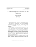
Figure 2.1 [1] shows TOSSIM’s architecture. TOSSIM consists of an Event Queue, Components Graphs, Radio Model, Communication Services, ADC Event, ADC Model and etc. In
the event-based network domain simulator, every sensor node’s behavior can be regarded as
a functional-level event. These events are kept in the simulator’s event queue in sequence
according to their timestamps. These events are processed in ascending order of their times9
Figure 2.1: TOSSIM architecture
tamps. When the simulation time arrives at one event’s timestamp, that event is executed
by the simulator. The Radio Model, Communication Services, ADC Event and ADC Model
are software programs that simulate the real life’s corresponding modules.
As an event based sensor network simulator, TOSSIM has following characteristics [14]:
• Fidelity
TOSSIM aims to provide a high fidelity simulation of TinyOS applications. The simulator is able to simulate packet transmission/reception and packet losses in the simulation. Furthermore, TOSSIM simulates communications at bit level that is more
accurate than ns-2 which simulates communications at packet level.
• Imperfections
TOSSIM cannot model interrupts correctly. On a real mote, an interrupt can fire no
matter other codes are running or not. However, as an event-driven simulator, an interrupt in TOSSIM simulation cannot fire until current running codes finish executing.
10
• Time
As a discrete event-driven simulator, TOSSIM only models event arrival time. It does
not model event’s execution time. This disables users so they cannot estimate and
analyze sensor motes applications’ real execution time.
• Building
TOSSIM modified the nesC compiler (ncc) to support the TinyOS application to be
compiled either for TOSSIM simulation or for running on the real hardware platform.
• Networking
With continuous development of TinyOS and TOSSIM, so far TOSSIM is able to
simulate mica, micaz networking stack, including the MAC, encoding, timing and
synchronous acknowledgements.
TOSSIM is a widely used simulator in sensornet research community due to its higher scalability and more accurate representation of sensornet than NS-2 [1]. Even though TOSSIM
is able to capture network behaviors and interactions, for example packet transmission, reception and packet losses at a high fidelity, it does not provide enough details at cycle-level.
Therefore, TOSSIM cannot capture and compare the performance of various hardware designs and the software implementations of sensornet applications.
In addition, TOSSIM simulation results cannot be considered authoritative because TOSSIM
does not consider several factors that should be considered in real system. For example,
event’s execution time and correct hardware interrupt behavior as discussed above.
2.2.2
Cycle-level sensornet simulators
SENSE [11] is a component-based sensornet simulator written in C++ that adopts objectoriented idea. In other words, in SENSE development, a new component can substitute for
11
another component if they have the same function interfaces. This makes models in SENSE
reusable. The capability of simulating large networks is achieved by packet sharing model.
EmStar [12] is a software framework that emulates sensor nodes running Linux operating
system. Codes simulated in EmStar can be running on actual hardware. EmTOS [15], an
extension of EmStar, allows translating TinyOS applications to EmStar libraries, which can
be simulated in EmStar.
Both SENSE and EmStar are component-based simulators. When simulating different sensor
nodes, many components in the simulator kernel must be modified by the user manually,
which is not user-friendly. On the contrary, using SUNSHINE to simulate different sensor
nodes does not need to hack the simulator’s kernel. Users only need to specify sensor nodes’
components in the configuration step before starting simulation.
ATEMU, the first instruction-level simulator for sensor network, is a fine-grained tool written
in C computer language. ATEMU is able to emulate the operation of each individual sensor
node in the whole sensor network.
As shown in Figure 2.2, ATEMU consists of an AVR Emulator, a graphical debugger tool
(XATDB), a configuration specification File and several peripheral devices. AVR Emulator is in charge of executing instructions running on AVR. XATDB allows user to debug
application programs on the ATEMU emulator. The configuration specification File specifies the hardware platform. Peripheral devices are linked and communicated with the AVR
Emulator.
Even though ATEMU is able to simulate a whole sensor network, it executes slowly when
simulating large scale sensor networks.
Avrora is also an instruction-level sensor network simulator which is written in Java computer
language. Avrora simulates a network of motes with cycle accuracy.
As shown in Figure 2.3 [16], Avrora consists of an Interpreter, an Event Queue, several
12
Figure 2.2: ATEMU components architecture
Figure 2.3: Avrora software architecture
on-chip devices and several off-chip devices. The on-chip devices are communicated with
the Interpreter through Input/Output Register’s interfaces, while the off-chip devices are
controlled through hardware components’ pins or through Serial Peripheral Interface Bus
(SPI). The Event Queue, which stores time-triggered events, is in charge of interpreting
sensor nodes’ behaviors.
13
Avrora uses multi-threading techniques with an efficient synchronization schemes to guarantee different sensor nodes running on different threads can interact with each other based on
a correct causal relationship. Avrora achieves better scalability and faster simulation speed
than ATEMU.
ATEMU [5] and Avrora [6] are the existing sensornet simulators that venture out of the
event-based simulations in network domain. They provide cycle-accurate software domain
simulation to evaluate the fine-grained behaviors of software over AVR controllers of MICA2
sensor boards.
Though ATEMU and Avrora are cycle-level sensornet simulators, they can only simulate
Crossbow AVR/MICA2 sensor boards. They cannot accurately capture the impact of alternative hardware designs on the performance of sensornet applications. In other words,
they do not support flexibility and extensibility in hardware beyond very simple parameter
settings.
2.2.3
Comparisons of SUNSHINE with Existing Simulators
In this part, I made several comparisons between SUNSHINE and other existing network
simulators.
SUNSHINE provides true hardware flexibility where a user can make changes in hardware
design of sensor node’s platforms and verify his/her sensornet application’s feasibility. SUNSHINE is able to simulate different potential hardware architectures. For example, SUNSHINE can simulate a sensor board with an FPGA to handle heavy computational intensive
tasks, such as advanced data packets encryption/decryption and data packets compression.
This provides a new direction to sensornet design and enables network researchers to evaluate
their designs under different hardware platforms. SUNSHINE provides a valuable instrument
to both sensornet community and hardware development community.
14
Table 2.1: Comparison between simulators
XXX
XXX
Name
XXX
Aspect
XXX
HW Flexibility
& Extensibility
Hardware behavior
User-defined
Platform Architecture
User-defined
Application
User-defined
Network Topology
Applications
Cycle Accuracy
Transition between
event-based and
cycle-accurate simulator
TOSSIM
Avrora/ATEMU
SUNSHINE
No
No
Yes
No
No
No
No
Yes
Yes
Yes
Yes
Yes
Yes
Yes
Yes
1
No
≥1
Yes
≥1
Yes
No
No
Yes
Further, each existing simulator can only work in one domain. For example, NS-2 and
TOSSIM only work in event-based network simulation domain while ATEMU and Avrora
can only execute cycle-accurate simulations. While TOSSIM and NS-2 lose their simulation
fidelity due to the coarse simulation granularity, the all cycle-accurate simulations of ATEMU
and Avrora require long execution time. Different from these existing simulators, SUNSHINE
offers its user flexible middle ground between cycle-accurate and event-based simulations.
It can combine a variety of nodes that simulated at coarse event-level and nodes that are
simulated at fine cycle-level.
Finally, SUNSHINE offers ability to capture hardware behavior of sensor nodes. This unique
capability of SUNSHINE can get the finer details of interactions among hardware components
at even bit level, which is not explored in Avrora, ATEMU or TOSSIM.
Table 2.1 summarizes the differences between TOSSIM, Avrora, ATEMU and SUNSHINE.
As shown in Table 2.1, hardware flexibility is one of the most significant advantages of SUN-
15
SHINE. Also, SUNSHINE’s ability of capturing hardware behavior is another improvement
for sensornet simulators.
2.3
SYSTEM DESCRIPTION
SUNSHINE combines three existing simulators: network domain simulator TOSSIM [1],
software domain simulator SimulAVR [2], and hardware domain simulator GEZEL [3]. In the
following, we first briefly introduce these three simulators. Then, we introduce SUNSHINE’s
system architecture and its simulation process.
2.3.1
System Components
• TOSSIM
TOSSIM [1] is an event-based simulator for TinyOS-based wireless sensor networks.
TinyOS is a sensor network operating system that runs on sensor motes. TOSSIM
is able to simulate a complete TinyOS-based sensor network as well as capture the
network behaviors and interactions. TOSSIM provides functional-level abstract implementations of both software and hardware modules for several existing sensor node
architectures, such as the MICAz mote. In TOSSIM, an event-based network simulator, sensor nodes’ behaviors are regarded as functional-level events, which are kept in
TOSSIM’s event queue in sequence according to the events’ timestamps. These events
are processed in ascending order of their timestamps. When the simulation time arrives
at one event’s timestamp, that event is executed by the simulator.
Even though TOSSIM is able to capture the sensor motes behaviors and interactions,
such as packet transmission, reception and packet losses at a high fidelity, it does
not consider the sensor motes processors’ execution time. Therefore, TOSSIM cannot
capture the fine-grained timing and interrupt properties of software code.
16
• SimulAVR
SimulAVR [2] is an instruction-set simulator that supports software domain simulation
for the Atmel AVR family of microcontrollers which are popular choices for processors
in sensor node designs. SimulAVR provides accurate timing of software execution and
can simulate multiple AVR microcontrollers in one simulation. SimulAVR is also integrated into the hardware domain simulator in SUNSHINE, and through this integration, the detailed interactions between sensor hardware and software can be evaluated.
Currently, SimulAVR does not support simulation of sleep mode or wakeup mode of
sensor nodes. We have added sleep and wakeup schemes to provide simulation support
for energy saving mode of sensor networks.
• GEZEL
GEZEL [3] is a hardware domain simulator that includes a simulation kernel and a
hardware description language. In GEZEL, a platform is defined as the combination
of a microprocessor connected with one or more other hardware modules. For example, a platform may include a microprocessor, a hardware coprocessor, and a radio
chip module. To simulate the operations of such a platform, one has to combine software simulation domain, which captures software executions over the microprocessor,
and hardware simulation domain, which captures the behaviors of hardware modules
and their interaction with the microprocessor. GEZEL is able to provide a hardwaresoftware co-design environment that seamlessly integrates the hardware and software
simulation domains at cycle-level. GEZEL has been used for hardware-software codesign of crypto-processors [17], cryptographic hashing modules [18], and formal verification of security properties of hardware modules [19], etc. GEZEL models can be
automatically translated into a hardware implementation that enables a user to create his/her hardware, to determine the functional correctness of the custom hardware
17
TinyOS
application
Binaries for
TOSSIM
simulation
Binaries for
hardware
mote
ncc
GEZEL
Sensor
Node
Hardware
Specification
TOSSIM
Radio
Chip
Module
SimulAVR
Cycle-accurate
co-sim node
Peripherals
TOSSIM node
GEZEL & SimulAVR: cycle accurate
TOSSIM: event-driven
Figure 2.4: Software architecture
within actual system context and to monitor cycle-accurate performance metrics for
the design.
GEZEL is the key technology to enable a user to optimize the partition between hardware and software, and to optimize the sensor node’s architecture. With the support of
GEZEL, the simulator can capture the software-hardware interactions and performance
at cycle-level in a networked context.
2.3.2
System Architecture
SUNSHINE integrates TOSSIM, SimulAVR and GEZEL to simulate sensornet in network,
software, and hardware domains. A user of SUNSHINE can select a subset of sensor nodes to
be emulated in hardware and software domains. These nodes are called cycle-level hardwaresoftware co-simulated (co-sim) nodes and their cycle-level behaviors are accurately captured
by SimulAVR and GEZEL. Other nodes are simulated in network domain by TOSSIM and
only the high-level functional behaviors are captured. These nodes are named TOSSIM
nodes. SUNSHINE is able to run multiple co-sim nodes with TOSSIM nodes in one sim18
ulation. The network topology in the right part of Figure 2.4 illustrates the basic idea of
SUNSHINE. The white nodes are TOSSIM nodes, which are simulated in network domain,
while the shaded nodes are co-sim nodes, which are emulated in software and hardware
domains. When running simulation, these TOSSIM nodes and co-sim nodes interact with
each other according to the network configuration and sensornet applications. Cycle-level
co-sim nodes can show details of sensor nodes’ behaviors, such as hardware behavior, but
are relatively slower to simulate. TOSSIM nodes do not simulate many details of the sensor
nodes but are simulated much faster. The mix of cycle-level simulation with event-based
simulation ensures that SUNSHINE can leverage the fidelity of cycle-accurate simulation,
while still benefiting from the scalability of event-driven simulation.
The simulation process in SUNSHINE is illustrated by Figure 2.4. First, for co-sim nodes
that emulate real sensor motes, executable binaries are compiled from TinyOS applications
using nesC compiler (ncc) and executed directly over these co-sim nodes. This is because
co-sim nodes emulate hardware platform at cycle level. Therefore, TinyOS executable binaries can be interpreted by SimulAVR, the AVR simulation component of SUNSHINE,
instruction-by-instruction. At the same time, GEZEL interprets the sensor node’s hardware
architecture description, and simulates the AVR microcontroller’s interactions with other
hardware modules at every clock cycle. One of the hardware modules that GEZEL simulates is the radio chip module. This radio chip module provides an interface to TOSSIM,
which models the wireless communication channels. Through these wireless channels, cosim nodes interact with other sensor nodes, which are simulated either as co-sim nodes by
GEZEL and SimulAVR, or as functional-level nodes by TOSSIM. To maintain the correct
causal relationship, the interactions between TOSSIM nodes and co-sim nodes are based
on the timing synchronization and cross-domain data exchange techniques, which will be
introduced in Section 2.4.
19
Figure 2.5: SUNSHINE’s Network Design Flow: Configuration, Simulation and Prototype
2.3.3
Network Design Flow
The design flow of a sensornet application using SUNSHINE has three steps: configuration,
simulation and prototype. In the configuration step, a user of SUNSHINE needs to set
network, software and hardware configurations for the sensornet application. Network configuration is used to specify network topology, number of total network nodes, and number
of co-sim nodes that are simulated by SimulAVR and GEZEL. The remaining nodes that are
not specified as co-sim nodes are set to TOSSIM nodes by default. For co-sim nodes, software and hardware configuration are needed. To be specific, software configuration specifies
application software running on each co-sim sensor node. Hardware configuration is sensor
node’s hardware architecture which includes what components are on the nodes, as well as
what communication interfaces are used between the components.
20
Simulation step is launched after configuration. Since the network contains TOSSIM nodes
and co-sim nodes, the simulation contains Network Domain Simulation (simulating TOSSIM
nodes) and Software and Hardware Domain Simulation (simulating co-sim nodes) accordingly. In Network Domain Simulation, real application modules, abstract TinyOS modules
and abstract hardware modules are running on the nodes. To be specific, real network applications are running on the nodes simulated by TOSSIM. Since TOSSIM only simulates
sensor nodes’ applications at coarse-grained level, TOSSIM can only simulate sensor nodes
with abstract TinyOS modules and abstract hardware modules. In Software and Hardware
Domain Simulation, co-sim nodes are evaluated by real application modules, real TinyOS
modules and simulated hardware architecture. Different from nodes simulated by TOSSIM,
Real TinyOS Modules are simulated by SW & HW domain simulation at cycle-level accuracy.
We call SW & HW domain simulation as P-Sim for short. By cross-domain simulation, sensor
nodes’ hardware and software performance as well as network performance can be simulated
in SUNSHINE simulator.
After getting satisfactory simulation results, the prototype is ready to be realized. The binaries run on cycle-level co-sim nodes can be loaded to actual sensor boards. In detail, TinyOS
application is compiled to intermediate C file through nesC compiler and is then compiled
to binary images through microprocessor-related cross compiler. The binary images can be
loaded to the microcontroller on the sensor node. The GEZEL codes running on FPGA can
be first generated to VHDL codes and then be compiled to binary images through corresponding FPGA design tool. The binary images are loaded to the FPGA on the sensor node.
As a result, real application modules, real TinyOS modules and real hardware platforms can
be profiled on wireless sensor network environment.
21
2.4
CROSS-DOMAIN INTERFACE
In this section, we will discuss how we interface the three components of SUNSHINE, each
working in a different domain of simulation.
2.4.1
Integrate SimulAVR with GEZEL
GEZEL provides standard procedures to add co-simulation interfaces with instruction-set
simulators, such as simulators of ARM cores, 8051 microcontrollers, and PicoBlaze processor
cores, to form a hardware-software emulator.
In SUNSHINE, in order to let the simulated AVR microcontroller (simulAVR) exchange
data with the simulated hardware modules, we create cycle accurate hardware-software cosimulation interfaces in GEZEL according to the AVR microcontroller’s datasheet [20]. To
be specific, four cosimulation interfaces between GEZEL and simulAVR, including interfaces
to AVR’s core, source pin (output pin), sink pin (input pin) and A/D pin, are developed in
GEZEL kernel according to the I/O mechanisms provided by simulAVR. Once the interfaces
are established, data can be exchanged between GEZEL-simulated hardware entities and
simulAVR-simulated microcontroller.
With the support of GEZEL’s co-simulation interfaces, SUNSHINE is able to form an emulator (P-sim) to capture the hardware-software interactions and performance of sensor nodes.
P-sim combines the software domain simulator SimulAVR and the hardware domain simulator GEZEL.
2.4.2
Timing Synchronization
SUNSHINE integrates network simulator TOSSIM and hardware-software emulator P-sim
for the purpose of scalability. However, simulations in these three domains run at different
22
Execution time for
simulating a cycle
Simulation time
Infidelity caused by
time difference
Time in cyclelevel simulation
Execution time
for processing
an event
Time in eventlevel simulation
Event in network
domain simulation
Wall clock time
Figure 2.6: Simulation time in different domains
step sizes. Without proper synchronization, we can easily get mismatches in simulation time
between event-driven simulation and cycle-level simulation as shown by Figure 2.6. The
wall clock time is the time required by the simulator to complete a simulation, i.e., the
simulator’s run time. The simulation time is the simulator’s prediction of the execution time
of a sensornet application based on the simulation of the sensornet. As shown in Figure 2.6,
P-sim runs at cycle-level steps, where each simulation step captures the behaviors of an AVR
microcontroller or a hardware component at one clock cycle. Therefore, the simulation time
is gradually increasing. However, in TOSSIM, a discrete event simulator, each simulation
step captures the occurrence and handling of a network event. As the time durations between
events are irregular, the simulation time in TOSSIM also increases at irregular steps. This
difference in simulation time may cause potential violations in causal relationship among
different sensor nodes in simulation.
To solve this issue, SUNSHINE includes a time synchronization scheme as depicted in Figure 2.7. In the design, TOSSIM uses the Event Scheduler to handle all the network events
while P-sim uses the Cycle-level Simulation Engine to control the simulation of hardware
23
modules and the AVR microcontroller every clock cycle. All network events are in the Event
Queue and are sorted according to their timestamps that record their occurrence time. The
Event Scheduler processes the head-of-line (HOL) event in the Event Queue only when the
Cycle-level Simulation Engine has progressed to the event’s timestamp. By selecting either
an event or a cycle-level simulation to be simulated next, SUNSHINE will maintain the
correct causality between different simulation schemes in the whole network.
Event Queue
Event
Scheduler
pop the
head-ofline event
Active Node List
run next cycle
run next event
Node 4
Node 5
timestamp of the
head-of-line event (t1)
Yes
Cycle-level
Simulation
Engine
time for executing
the next cycle (t2)
t1 < t 2
proceed to
the next
cycle
No
Figure 2.7: Synchronization Scheme
The design in Figure 2.7 also provides synchronization supports for co-sim nodes in sleep
mode by maintaining an Active Node List. This list holds the active nodes that need to
be simulated with cycle-level accuracy. The Event Scheduler adds or removes nodes from
the list upon node wakeup or node sleep events. At each cycle-level simulation step, the
Cycle-level Simulation Engine only processes a clock cycle for the nodes of the Active Node
List. As a result, a node’s sleep or wakeup state does not need to be checked every clock
cycle. Given the fact that in sensornets, a sensor node spends most of its time in sleep mode,
this design will greatly accelerate SUNSHINE’s simulation speed.
Based on the synchronization scheme, the desired behavior of a synchronized simulation can
be achieved as shown in Figure 2.8. Events in the network domain are processed with the
correct causal order compared to the cycle-level simulation, and the SUNSHINE simulator
correctly interleaves cycle-level processing with event-driven processing.
24
Simulation time
Switching from cycle-level
simulation domain to
network simulation domain
Switching from
network domain
simulation to
cycle-level
simulation
domain
Time in cyclelevel simulation
Time in event-level
simulation
Event in network
domain simulation
Node sleeping
event
Node wakeup
event
Wall clock time
Figure 2.8: The synchronized simulation time in SUNSHINE
2.4.3
Cross-Domain Data Exchange
Since SUNSHINE integrates simulation engines working in three different domains, it is
necessary to implement interfaces for cross-domain data exchange between these simulators.
The data exchange between SimulAVR and GEZEL is explained in Section 2.4.1. In this
section, we focus on discussing how data exchanges between hardware-software emulator
P-sim with event-based simulator TOSSIM.
Noise Models
A wireless network simulator needs to build radio and noise models to simulate wireless
packet delivery. Since SUNSHINE integrates P-sim with network simulator TOSSIM, it is
convenient to adopt TOSSIM’s radio model to simulate wireless packet transmission and
reception. TOSSIM also uses the closest-fit pattern matching (CPM) noise model [21] to
simulate whether the packets can be successfully received from the channel.
25
Since TOSSIM simulates high functional level network behavior, if there is a collision of the
packets in the channel (i.e., two nodes send packets to the third node at the same time),
TOSSIM simply assumes that the packets are corrupted and drops the packets. This is
different from the real radio chip. In reality, the radio chip performs Frame Check Sequence
(FCS) scheme to check whether the packet is received correctly and marks its CRC bit
accordingly [22].
To simulate the radio chip’s real performance in SUNSHINE, the CPM model is modified by
adding a receive FIFO (RXFIFO) to the radio chip module to store the received packets. In
the simulation, when the CPM model determines a node successfully receives a packet, the
received packet is stored in the RXFIFO with CRC bit set to 1 to demonstrate the packet is
received successfully without error. However, if the CPM model determines a node receives
a corrupted packet, the RXFIFO stores the received data with CRC bit set to 0 to mention
that the data is not received correctly. This process is in accordance with the real radio
chip’s behavior [23].
Event Converter
Sensor nodes in network domain simulated by TOSSIM need to exchange messages with
nodes in software-hardware domain simulated by P-sim through the TOSSIM simulated
channel. However, network domain simulation and hardware-software domain emulation
have different simulation abstractions. For TOSSIM, it abstracts the functions and interactions among network components as high-level abstracted events. For example, as shown
in Figure 2.9, the transmission or reception of an entire packet is regarded as a single event
in TOSSIM. In hardware-software domain emulation, the packet transmission and reception
related functions and interactions among hardware modules are simulated as series of behaviors in many cycles. For example, to simulate the reception of a packet, the bits received
26
and read from the radio chip module should be simulated at each clock cycle. Therefore, a
time converter is needed to bridge this gap in time granularity.
A packet reception
event
Node simulated
in functional level
Bytes received by the radio
chip at each clock cycle
Event
converter
TOSSIM
Node simulated
in cycle level
GEZEL & SimulAVR
Figure 2.9: Converting a functional-level event to cycle-level events
Another issue is the message format defined in TOSSIM is different from the message format
in the real mote according to the radio chip’s datasheet [3]. Therefore, a packet converter is
built to facilitate the conversion of packets between TOSSIM and P-sim.
Figure 2.10 illustrates the event conversion process. If a co-sim node transmits a data packet,
it should follow several steps in simulation. The simulated AVR microcontroller first sends
the packet to the radio chip module at cycle level. The radio chip module stores the packet
in a transmit FIFO (TXFIFO). As soon as the radio chip module receives a send command
from the simulated microcontroller, the time converter transforms P-sim’s simulation time to
TOSSIM’s simulation time, while the packet converter changes the real mote’s packet format
to TOSSIM’s packet format, and sends the packet to the TOSSIM simulated channel. Based
on this scheme, both TOSSIM nodes and co-sim nodes in the receiver side are able to receive
the packets from the sender.
If an event that indicates a co-sim node to receive a packet from the TOSSIM simulated
channel is fired from the Event Queue, the packet converter modifies the abstract TOSSIM
packet to the real bytes of the packet, and puts these bytes into the RXFIFO of the radio
chip module. In addition, the time converter converts TOSSIM’s current event time to
several detailed simulation time, such as the start of frame delimiter (SFD) time, the length
27
TOSSIM
Radio Chip Module
Simulated AVR
event queue
Packet
transmission
event
Packet
reception
event
RXFIFO
Cycle
Accurate
(1 bit/cycle)
Event
converter
registers
TXFIFO
Figure 2.10: Event conversion process
field time, etc, on the basis of the radio chip’s datasheet [23]. These timing information are
provided for the simulated AVR microcontroller to read data from the RXFIFO according
to the datasheet [23].
Using the event converter, SUNSHINE is able to convert coarse packet communication events
to the cycle-level packet reception and transmission behaviors and vice versa. Based on
this mechanism, SUNSHINE satisfies both P-sim’s cycle-level and TOSSIM’s event-level
requirements.
2.5
HARDWARE SIMULATION SUPPORT
As SUNSHINE is able to simulate hardware behavior, in this section, we discuss SUNSHINE’s
support for hardware simulation.
2.5.1
Hardware Specification Scheme
One of the primary contributions of SUNSHINE is to support hardware flexibility and extensibility. SUNSHINE describes sensor motes hardware architecture at simulation’s configuration level using GEZEL-based hardware specification files. Users of SUNSHINE can
make various modifications to sensor motes architecture, such as using different microcontrollers, adopting multiple microcontrollers, adding hardware coprocessors, connecting with
28
new peripherals and performing other customizations on the platform. The syntax of a valid
hardware specification file based on GEZEL is relatively simple. Users are able to write their
own specification files according to GEZEL semantics [24].
To demonstrate this point, Figure 2.11 shows specific details of how hardware architecture
of a MICAz mote is described in SUNSHINE. We listed a snippet of the hardware specification file in Figure 2.11. The file is divided into three pieces, each of which is dedicated
to a relevant hardware part. From the code snippet, we would see that users could pick
hardware components using “iptype” statements to configure a sensor node’s hardware platform. In this specific example, microcontroller Atmega128L and radio chip CC2420 are
chosen to form the MICAz hardware platform. The components’ corresponding ports are
interconnected through virtual wires that are also described in the specification file. For
example, “Atm128sinkpin” wires the input pin B3 of the AVR microcontroller’s core to the
output pin MISO of the CC2420 chip, while “Atm128sourcepin” wires the output pin B0 of
the AVR microcontroller’s core to the SS input pin of the CC2420 chip. While our example shows the MICAz platform, a user can also pick other components to form a different
hardware platform in their sensornet simulation. For example, one can use ARM or 8051
microcontroller instead of Atmega128L by modifying the hardware specification file. Based
on this mechanism, SUNSHINE can easily combine different hardware components to form
different hardware platforms for sensornet simulation. In other words, SUNSHINE supports
running network simulation over flexible hardware platforms that are created based on either
commercial off-the-shelf sensor boards or the user’s customized platform designs.
The example in Figure 2.11 also shows how SUNSHINE enables different co-sim nodes to
run different software applications through the use of “ipparm” statements. The “ipparm”
can also be used to set parameters for hardware components. In Figure 2.11, the statement ipparm “exec = app” means the simulated AVR microcontroller would interpret the
executable binary named ”app”, which is compiled from a software application using ncc
29
compiler. Users can also configure the simulated AVR microcontroller to execute other binaries in a co-sim node through ipparm statements. By configuring different co-sim nodes to
execute different software binaries, SUNSHINE can simulate a sensornet that has multiple
different applications. This is a significant improvement over TOSSIM, which can only run
one application in a whole network. Essentially, SUNSHINE’s simulation configuration steps
are as follows. First, the executable binaries of applications are compiled from their source
codes. Then, as shown in Figure 2.11, a Hardware Specification file is created to describe
how hardware components form the hardware platforms in the sensornet. The Hardware
Specification file also links the generated executable binaries to the corresponding hardware
platforms. After the configuration, SUNSHINE simulation can start.
TinyOS executable
binary named ``app '’
LED0
LED1
LED2
B7
E6
D6
D4
A1 ATmega128
B0
B1
A0
B2
B3
FIFO
FIFOP
CCA
SFD CC2420
SS
SCK
MOSI
MISO
A2
ipblock avr{
iptype ``atm128core '’;
ipparm``exec=app'’;
}
Hardware
Specification
file
ipblock m_miso (out data: ns(1)){
iptype ``atm128sinkpin '’;
ipparm ``core=avr '’;
ipparm ``pin=B3 '’;
}
ipblock m_ss (out data : ns(1)) {
iptype "atm128sourcepin";
ipparm "core=avr";
ipparm "pin=B0";
}
ipblock m_cc2420 (out fifo,fifop,cca,sfd:ns(1);
in ss,sck, mosi:ns(1);
out miso:ns(1)){
iptype``ipblockcc2420'’;
}
Figure 2.11: Hardware specification for a single node. Multiple nodes can be captured by
instantiating multiple AVR microcontrollers and multiple radio chip modules.
From the above description, one would see that SUNSHINE can be used to simulate various
hardware platform designs to find the most suitable hardware module for a given network
environment and a given set of application requirements. Therefore, SUNSHINE is an efficient tool to help hardware designers develop better sensor motes. In addition, researchers
30
in the field of software can also use SUNSHINE to easily configure novel hardware architectures and then evaluate their sensornet applications and protocols over these customized
architectures. Because SUNSHINE can change hardware components easily at simulation’s
configuration level, even software researchers with little hardware knowledge can configure
sensornet hardware platforms themselves.
2.5.2
Hardware Behavior
Unlike other sensornet simulators, SUNSHINE is able to accurately capture sensor nodes’
hardware behaviors. Users are able to know whether the microcontroller is in sleep mode
or active mode as well as identify the radio chip’s current radio control state. In addition,
through interpreting GEZEL code, a hardware description language, SUNSHINE is able
to display cycle-level behavior of hardware components when applications are running on
co-sim nodes. This would help hardware designers know how hardware module behaves in
sensornet applications.
Figure 2.12: Traces for TinyOS Reception application
For example, users can track hardware pins’ activities when running a sensornet application
31
on a co-sim node in SUNSHINE by doing the following. The signal tracing mechanism of
SUNSHINE records stimuli files when the simulation is set in debug mode. These stimuli
files, named Value-Change Dump (VCD) files, can be read by digital waveform viewing tools,
such as GTKWave, to produce graphic illustrations of hardware pins’ values. An experiment
is provided to show SUNSHINE’s capability of capturing the sensor nodes’ hardware performance. In the experiment, a TinyOS Transmission application runs on one co-sim node and
the Reception application runs on the other co-sim node. In the Transmission application,
the sensor node keeps sending packets to the radio channel using the largest message payload
size. In the Reception application, the node listens to the channel and receives packets from
the channel. Figure 2.12 shows detailed activities of the hardware pins at the receiving node.
Through these traces, users are able to detect how the AVR microcontroller interacts with
the CC2420 radio chip.
2.6
Debugging Methods for Sensornet Development
Even though GNU debugger gdb is a common debugging method for programs running in
Linux, it is inefficient to debug large programs especially the programs that contain many
library blocks such as dynamic-link libraries. In the following, we will present the debugging
methods that SUNSHINE provided to facilitate the development of sensornet applications.
These methods are not only helpful for debugging sensornet applications, but are also suitable
for tracing sensor nodes’ cycle-accurate activities in the simulator.
2.6.1
Debugging Methods for Sensornet Software Applications
In TOSSIM, a debugging output system [25] is provided to debug TinyOS applications
via printing desired statements out in simulation by adding “dbg” in TinyOS applications.
Since TinyOS applications are built above TinyOS libraries that hide all the low-level device
32
drivers’ codes, debugging programs at device driver level is impossible using the “gdb”
debugging scheme.
To solve this problem, a debugging method is provided in SUNSHINE simulator to accurately
trace the behaviors of sensor node’s program’s cycle-accurate activities in simulation not
only at application program level but also at low level device drivers. The debugging tool
leverages the fact that common sensor nodes’ microprocessors such as Atmega 128Ls have
reserved registers that are not used by sensor programs. We use two “reserved” registers’
memory addresses [20] to store input and output streams respectively. By using reserved
registers’ memory addresses, we essentially avoid contending the same memory addresses
with sensornet application programs in the debugging process. The output messages can be
shown on the screen by including microprocessor-based libraries.
To debug a sensornet program using this method, a programmer first adds debugging statements to desired places in either TinyOS application (nesC file) or in the intermediate C
file generated from the TinyOS application by nesC compiler. Then, one compiles the sensornet program and runs the compiled code over SUNSHINE simulator. The corresponding
debugging messages will be printed out in the screen during the SUNSHINE simulation. As
a result, users can accurately trace the program’s procedure based on the debugging output
in SUNSHINE.
Figure 2.13 shows an example for using the debugging method in an intermediate C file generated from a TinyOS application written in nesC. In the example, the debugging statements
are added to the main function. Figure 2.14 shows the output messages on the screen while
running simulation in SUNSHINE. The statements can be added to other places in the C
file according to debugging requirements.
33
Figure 2.13: Debugging statements added to code snippets of the intermediate C file
2.6.2
Debugging Method for Hardware Components
SUNSHINE not only provides the method for debugging software program running on sensor
platforms, it also provides a method to trace the activities of hardware components in a sensor
platform to help debug hardware designs. In the following, we will use wireless transceiver
(radio) to illustrate SUNSHINE’s hardware debugging method. Wireless transceiver is an
essential component of a sensor platform and its behavior depends on wireless channel status.
To trace the behavior of the radio component, a debugging on/off switch is added as a macro
into the radio’s module. If the debugging switch in the module is turned on, the activities
34
Figure 2.14: Simulation results using the debugging method
of the radio can be printed out. Otherwise, no debugging messages for the radio are shown
on the screen.
Figure 2.15 shows the screen shot of the activities of a sensor node’s radio for running a
transmission application that broadcasts a packet with three-byte payload. As shown in
the figure, the behaviors of the radio, such as when and what command strobes received
from the microprocessor, when and what packets’ bytes received from the microprocessor,
packet transmission’s start and end time, etc. , are shown at cycle level through SUNSHINE
simulation. Since there is a tradeoff between displaying debugging details and simulator’s
runtime efficiency, it is recommended to show only essential messages when simulating large
sensor networks.
Based on the debugging methods provided in SUNSHINE, sensor nodes’ detailed activities
can be profiled at cycle level.
2.7
EVALUATION OF SUNSHINE
We performed the experiments on a Dell laptop that has Intel (R) Core (TM) 2 Duo CPU
T5750 @ 2.00GHz, 3G RAM and runs Linux 2.6.32-23-generic. SUNSHINE integrates
TinyOS version 2.1.1, SimulAVR and GEZEL version 2.5. We used the latest version of
35
Figure 2.15: Screen shot for the transmission application using a co-sim node
the simulators available at the time of performing the experiments. The hardware platform
configured in these simulations is MICAz.
2.7.1
Scalability
In the following, we simulated several applications to analyze SUNSHINE’s scalability. In
the first application, we varied the number of nodes that are randomly distributed from 2 to
128. Nodes are paired to communicate with each other. We wrote an application to let the
paired nodes send packets between each other. The simulation ends when all of the nodes
receive one message from its neighbor. We considered four cases: the first case is pure co-sim
36
50
wall clock time (s)
40
100% co−sim nodes
50% co−sim nodes
25% co−sim node
100% TOSSIM nodes
30
20
10
0
0
20
40
60
80
100
120
number of nodes
Figure 2.16: Scalability
nodes network, the second one is pure TOSSIM nodes network, the third is the combination
of 50% co-sim nodes with 50% TOSSIM nodes network, and the fourth is 25% co-sim nodes
with 75% TOSSIM nodes network.
Figure 2.16 shows SUNSHINE’s wall clock time which represents the time required by SUNSHINE to complete the simulation. As expected, pure TOSSIM simulation outperforms
SUNSHINE in terms of simulation speed by abstracting away the detailed behaviors of sensor nodes, such as hardware clock cycles and microprocessor’s instructions. On the other
hand, SUNSHINE’s low execution speed comes from its fine-grained simulation accuracy.
Moreover, Figure 2.16 shows that SUNSHINE has the ability of simulating hybrid network
consists of co-sim nodes and TOSSIM nodes. When simulating the mixed network, SUNSHINE’s execution speed is accelerated and hence can be suitable for even large networks.
Figure 2.17 shows the memory utilization of the simulation. The simulation with 100% cosim nodes utilizes large CPU memory because cycle-level simulation needs to cache a lot
37
7
memory utilization (kilobytes)
14
x 10
12
10
100% co−sim nodes
50% co−sim nodes
25% co−sim nodes
100% TOSSIM nodes
8
6
4
2
0
0
20
40
60
80
100
120
number of nodes
Figure 2.17: Memory Utilization
of co-sim nodes’ data and states from GEZEL, simulAVR and TOSSIM. These data and
states can take a large amount of memory space when simulating a large network. To reduce
the memory consumption, SUNSHINE can combine TOSSIM nodes with co-sim nodes to
decrease the memory utilization.
Given these information, combining co-sim nodes with TOSSIM nodes becomes an advantage
of both speeding up the simulator’s run time and decreasing memory usage. Also, this
combination is acceptable since in most network scenarios, only important nodes need to
be simulated at cycle-level fine granularity (i.e. simulated as co-sim nodes) to evaluate
their hardware and software performance. Other nodes, whose detailed behaviors are not
important, can be simulated in TOSSIM. Several specific examples are given as follows.
• Ring Network
We simulated a packet relaying application based on a 320 nodes’ ring network. In
the packet relaying application, the first node sends a packet with two bytes payload
38
length to the next hop. As soon as the second node receives the packet from the
previous one, it forwards the same packet to the next node. The application ends
when the first node receives the two bytes packet from its previous node. In this case,
most of the sensor nodes have the same behaviors (e.g. receiving and forwarding the
data to another node). Since co-sim nodes are used to analyze sensor nodes’ cycle
level software-hardware performance, only simulating a few co-sim nodes is sufficient
to analyze the network behavior. In this experiment, we used 5% co-sim nodes and 95%
TOSSIM nodes to consist the network. We randomly chose co-sim nodes’ positions in
order to show the interconnection between TOSSIM and co-sim nodes. We simulated
the application ten times with different co-sim nodes’ positions and calculated the
average of the simulator’s run time. In the experiment, simulating 320 nodes only takes
217.35s. Using ring network avoids packets collisions in the channel. Dense networks
are deployed to illustrate SUNSHINE’s performance in the following experiments.
• Star Network
2
3
9
8
1
7
4
5
6
Figure 2.18: Star Network
A nine nodes’ star network is simulated in SUNSHINE. The network topology is shown
in Figure 2.18, which includes one base station placed at the center, that receives data
39
from other nodes, and eight normal sensors, that take turns to send one packet to the
base station. The simulation ends when the base station receives all the leaf nodes’
packets. In this application, to analyze fined-grained network behavior, we only need
to simulate the base station and one leaf node as co-sim nodes, while other leaf nodes
can be set to TOSSIM nodes. SUNSHINE finishes simulation in 3.71s using two co-sim
nodes, compared to 19.75s run time using all (nine in this case) co-sim nodes.
• Tree Network
16
13
1
2
3
14
4
5
6
7
15
8
9
10
11
12
Figure 2.19: Tree Network
A three-layered tree network is considered as shown in Figure 2.19. Nodes 1 to 12 send
packets to their parent nodes, 13 to 15, respectively. After receiving the packets from
all their children nodes, nodes 13 to node 15 first perform several computational tasks
(e.g. compressing the data received from its children nodes) and then send the packets
to the root node 16. As soon as node 16 receives the packets from nodes 13 to 15,
simulation ends. Since in a real sensor network, the bottleneck node is highly likely
to be node 16, to investigate the bottleneck node’s behavior under heavy load, it is
reasonable to simulate the root node 16 as co-sim node. In addition, several nodes that
perform computational tasks and can become overloaded, such as nodes 13 to 15, can
also be considered as co-sim nodes. In this experiment, simulating four co-sim nodes
40
Figure 2.20: Testbed: Five Nodes’ Ring Network
(nodes 13 to 16) with 12 TOSSIM nodes (nodes 1 to 12) takes 159.00s. However, using
the root node 16 as co-sim node while others (nodes 1 to 15) are TOSSIM nodes only
takes 24.64s.
According to the above experiments, we can draw a conclusion that SUNSHINE is able
to capture sensor nodes’ cycle accurate hardware-software performance while keep the
simulator’s execution speed fast by mixing co-sim nodes with TOSSIM nodes in the
network simulation. Therefore, users should choose important nodes as co-sim nodes
running at cycle level, while other nodes as TOSSIM nodes to ensure SUNSHINE’s
simulation can scale to large networks.
2.7.2
Simulation Fidelity
In this section, we conducted two real-mote experiments on Crossbow MICAz OEM reference
boards to show the simulation fidelity of SUNSHINE. Each result is the average value of ten
experiment runs.
41
Figure 2.21: Testbed: Two Nodes’ Network
In the first experiment as shown in Figure 2.20, we deployed a five node sensor network to
analyze SUNSHINE’s channel performance. Since SUNSHINE utilizes the TOSSIM’s radio
and noise models which have been validated in [1, 21], in this experiment, it is sufficient to
consider a simple ring network topology with a focus on packet relaying applications (that
are introduced in Section 2.7.1).
As measured in real motes, the average time of a round trip is 76.5 ms, which is close to
that of using SUNSHINE, i.e., 70.62 ms (both values are measured without ack). As can be
inferred from the results, SUNSHINE is able to provide fairly reliable results as reference for
the sensor network applications.
In the second experiment, we evaluated SUNSHINE’s capability of executing computational
tasks. On the testbed as shown in Figure 2.21, we ran the TinyOS Transmission application
(mentioned in Section 2.5.2). The sensor node executes a dummy computational task of
multiple empty loops before sending packets to the other node, and we varied the number of
empty loops to represent various levels of computation intensity. We compared SUNSHINE,
42
4.5
4
3.5
SUNSHINE
real mote
TOSSIM
time (s)
3
2.5
2
1.5
1
0.5
0
−0.5
0
1
2
3
computation intensity (loops)
4
5
x 10
Figure 2.22: Validation Results
TOSSIM and the real mote in terms of the task execution time in simulation/experiment,
and the results are shown in Figure 2.22.
From the results, we are able to observe that (1) TOSSIM runs fastest as expected, and
its predicted task execution time is much less than the real task execution time; and (2)
SUNSHINE is able to provide a simulated task execution time that coincides with that of
the real mote experiment. TOSSIM’s fast simulation speed is attributed to its inability of
capturing the task execution time on the microcontroller, which will apparently limit its
applicability for time-sensitive applications/protocols. Many security protocols, such as the
distance-bounding protocol [26], require precise time-out behavior to thwart physical manin-the-middle attacks. When testing and verifying these protocols, SUNSHINE will outcompete TOSSIM since SUNSHINE is able to correctly capture the impact of computation
intensity on sensornet performance.
43
2.8
Conclusion
In this chapter, we have presented SUNSHINE, a novel simulator for the design, development and implementation of wireless sensor network applications. SUNSHINE is realized by
the integration of a network-oriented simulation engine, an instruction-set simulator and a
hardware domain simulation engine. By the seamless integration of the simulators in different domains, the performance of network protocols and software applications under realistic
hardware constraints and network settings can be captured by SUNSHINE with networkevent, instruction-level, and cycle-level accuracy. SUNSHINE outperforms other existing
sensornet simulators because it can support user-defined sensor platform architecture, which
is a significant improvement for sensornet simulators. SUNSHINE can also capture hardware
behavior which is the unique feature of sensornet simulators. SUNSHINE serves as an efficient tool for both software and hardware researchers to design sensor platform architectures
as well as develop sensornet applications.
44
Chapter 3
Simulating Power/Energy
Consumption of Sensor Nodes in
Wireless Networks
3.1
Introduction
Nowadays, WSNs are proposed to be used in many applications, such as structure and
environment monitoring, health care, and so forth. In the past, these WSNs were composed of
sensor nodes that mainly consist of a microcontroller and a wireless transceiver. However, the
microcontroller’s processing capability may cause a real-time bottleneck when sensor nodes
have to execute compute-intensive tasks, such as message encryption/decryption and large
data compression/decompression. To accelerate the execution speed of the sensor nodes,
adding a hardware accelerator to form a flexible sensor node has been recently proposed
in [27] [28].
Apart from fixed components, such as a transceiver and a microcontroller, a flexible sensor
node has a programmable hardware component, i.e., FPGA. In contrast to the fixed sen45
sor node whose hardware functionalities, such as circuitry, clock frequency and I/O ports
are fixed, the programmable logic of FPGA can be configured to perform either complex
algorithms by programming thousands of logic cells or simple calculations that just uses one
AND or OR gate. Based on this functionality, executing compute-intensive tasks in parallel on FPGA instead of sequentially on microcontroller can make the flexible sensor node’s
execution speed orders of magnitude faster than the fixed sensor node’s.
Due to the high cost of building, deploying and debugging distributed sensor network prototypes in real environments, it is better to evaluate applications in simulation before deploying
applications on actual WSNs. Unfortunately, no simulators have been developed to evaluate
the real-time performance and energy consumption of such flexible platforms. Therefore, it
is difficult to identify what specific applications can benefit from flexible platforms in large
WSNs.
To evaluate the real-time performance of flexible platforms, in our previous work, we built
SUNSHINE [4]. SUNSHINE is a cycle-accurate simulator that can emulate the behaviors
of flexible sensor nodes in wireless networks. While we have demonstrated that SUNSHINE
can accurately capture the timing behaviors of WSNs’ applications on flexible hardware
platforms, estimating their power/energy consumption has turned out to be very challenging
and has remained unsolved until this work.
Predicting the power consumption for flexible sensor nodes is challenging for two reasons.
First, predicting the power/energy consumption of fixed (microcontroller) and flexible (FPGA)
components’ interactions in wireless network environment is difficult. Second, the power estimation processes for fixed and flexible components are completely different from each other.
Because of the above challenges for estimating power consumption of flexible nodes, existing power estimation tools [29][30] only support fixed sensor nodes. The lack of capability
on analyzing power consumption of flexible nodes would result in restricting analysis and
development of flexible sensor platforms in large networks.
46
The focus of this chapter is to describe our novel design of a power/energy estimation tool
called PowerSUNSHINE for WSNs. PowerSUNSHINE is able to predict power/energy consumption of not only fixed-platform sensor nodes, such as MicaZ nodes, but also flexible
sensor nodes with reconfigurable FPGAs. To the best of our knowledge, PowerSUNSHINE
is the first to provide power/energy estimation of flexible sensor nodes.
Our major contributions are summarized as follows.
1. We developed a methodology for estimating power/energy consumption of flexible sensor platforms in wireless network environment. Based on this method, power/energy
consumption models for each component, including microprocessor, radio transceiver,
and FPGA-based component, are established, so that a wide range of sensor platforms’ power/energy consumption can be captured by combining the power/energy
consumption of their components.
2. Following our methodology, we built a power/energy modeling extension, called PowerSUNSHINE, into the SUNSHINE simulator. Unlike other power tools that only
evaluate fixed hardware platforms, PowerSUNSHINE supports both fixed and flexible
sensor platforms.
3. We set up two testbeds, a MicaZ platform and a flexible sensor platform with a FPGAbased co-processor, to evaluate the fidelity of PowerSUNSHINE.
The rest of the chapter is organized as follows. Section 3.2 presents related work of power
tools for wireless sensor networks. Section 3.3 first introduces the architecture of SUNSHINE, and then presents PowerSUNSHINE’s characteristics, architecture, and challenges.
Section 3.4 presents power/energy models of fix-function components. Section 3.5 discusses
power/energy models of reconfigurable components. Section 3.6 provides the setup of actual
hardware platforms. Section 4.8.3 offers evaluation results of PowerSUNSHINE. Finally,
Section 4.9 provides conclusions.
47
3.2
Related Work
To measure actual sensor nodes’ power consumption directly, several papers [31] [32] measured actual sensor nodes’ current at real-time via specialized circuits. Even though these
methods have high-precision results, building hundreds of circuits to measure large WSNs’
power/energy turns out to be time-consuming and impractical. In such a case, building a
system to estimate the WSNs power/energy consumption is crucial in the area of sensor
networks.
Several simulation tools for energy profiling of sensor nodes have been developed in existing
work. For example, PowerTOSSIM [29] has been built on top of TOSSIM simulator to
estimate Mica2’s energy consumption. Since TOSSIM cannot emulate a microcontroller’s
execution time, to estimate the microcontroller’s power consumption, PowerTOSSIM has to
estimate microcontroller’s execution time based on the intermediate C code generated by
tinyOS applications. This estimation, however, may be fairly inaccurate in many cases. By
comparison, in PowerSUNSHINE, the microcontroller’s cycle counts are precisely counted
by SUNSHINE. Therefore, the microcontroller’s energy consumption can be more accurately
captured.
AEON [30] is developed based on a cycle accurate simulator AVRORA to profile Mica2’s
energy. AEON breaks down Mica2’s components and calculates each hardware’s energy in
the system. AEON is able to capture Mica2 nodes’ power consumption accurately since
AVRORA can simulate microcontroller’s cycle-accurate behavior.
However, since AEON’s ability of capturing cycle-accurate sensor nodes behavior, the simulator’s run time is fairly slow. In addition, if one large network is only interested in several
particular nodes power consumption, AEON still has to simulate the large network, evaluate
every node cycle by cycle, and estimate all the nodes power consumption. This simulation
48
method would limit the scalability of AEON. In contrast, PowerSUNSHINE would scale to
large networks since SUNSHINE can combine the event-based network simulator TOSSIM
with the cycle-accurate sensor network simulator P-sim to scale to simulate large sensor
networks [4].
None of PowerTOSSIM or AEON is able to evaluate the power consumption of flexible sensor
nodes. They are dedicated for fixed sensor nodes. PowerSUNSHINE is able to capture both
fixed and flexible sensor nodes’ power consumption.
3.3
PowerSUNSHINE Overview
In this section, we first briefly introduce the architecture of SUNSHINE, which is the foundation of PowerSUNSHINE. Then, we describe the characteristics, architecture and challenges
of PowerSUNSHINE.
3.3.1
SUNSHINE Simulator
PowerSUNSHINE’s ability to profile the power consumption of fixed and flexible sensor nodes
is based on SUNSHINE, a cycle-accurate hardware-software simulator for sensor networks.
SUNSHINE is developed by the authors in their previous efforts and is the only existing simulator that can simulate flexible sensor platforms. Other existing sensor network simulators
can only capture fixed hardware platforms and do not support simulation of reconfigurable
hardware designs. In the following, we give an overview of SUNSHINE.
Fig. 3.1 illustrates SUNSHINE’s software architecture [4]. A sensor node can be simulated
by SUNSHINE in two different modes: co-sim mode or TOSSIM mode. For nodes simulated
in TOSSIM mode (called TOSSIM nodes), only high-level functional behaviors are captured
while for nodes in co-sim mode (called co-sim nodes), the behaviors of hardware co-processors
49
Figure 3.1: SUNSHINE software architecture
are described by a hardware description language, GEZEL [24] and are simulated at cyclelevel accuracy. The cycle-accurate behaviors of other components in co-sim nodes, such as
microcontrollers and transceivers, are also captured in SUNSHINE.
With the support of SUNSHINE, especially its ability of simulating accurate behaviors of
co-sim nodes, building a power/energy estimation tool for both fixed and flexible sensor platforms in network environment becomes feasible. Furthermore, building PowerSUNSHINE
over SUNSHINE simulator has the following advantages:
• Accuracy:
SUNSHINE accurately captures the behaviors of sensor nodes at cycle level. This
provides the foundation to ensure that the power/energy consumption of sensor nodes
estimated by PowerSUNSHINE is close to the measurement results of actual boards.
• Flexibility:
Based on SUNSHINE’s capability to simulate arbitrary hardware platforms, Power50
SUNSHINE supports estimating power/energy consumption of different sensor platforms.
• Compatibility:
Since TinyOS applications can run in SUNSHINE, PowerSUNSHINE can profile power/energy consumption of sensor nodes running TinyOS applications directly. This is
useful because TinyOS is the dominating operating system for WSNs.
• Path to Implementation:
Both SUNSHINE and PowerSUNSHINE bridges the gap between design and implementation of flexible sensor nodes’ applications. The applications evaluated by SUNSHINE
and PowerSUNSHINE in simulation can be loaded and run on actual hardware.
3.3.2
PowerSUNSHINE Architecture
Building a power/energy simulation model for flexible hardware platforms (with fixed hardware platform as a special case) is a non-trivial task. PowerSUNSHINE aims to capture a
wide range of possible platform designs that are formed by different combinations of hardware components. Thus, power models based on measurement of the power consumption of
existing platforms as a whole will not work, since one platform cannot represent the power
consumption of another platform with different hardware designs.
To solve this problem, PowerSUNSHINE decomposes the power consumption of a sensor platform into a combination of power consumption of individual hardware components. Fig. 3.2
illustrates the block diagram of PowerSUNSHINE architecture. PowerSUNSHINE is associated with co-sim nodes, whose cycle accurate hardware-software behaviors are captured by
SUNSHINE. When SUNSHINE is simulating applications of sensor nodes, PowerSUNSHINE
breaks down sensor nodes into components, calculates power/energy consumption of each
component, and then adds all the components power/energy consumption together.
51
Figure 3.2: Block diagram of PowerSUNSHINE architecture
To be specific, if PowerSUNSHINE is applied for fixed sensor nodes in the simulation, it
tracks cycle accurate activities of every component, and uses the power/energy model to
calculate the total power/energy consumption of the nodes according to their components’
activities.
Compared with fixed nodes, a flexible node has an extra programmable FPGA. If PowerSUNSHINE is applied for the flexible node, the additional power/energy dissipation of
FPGA should be considered. Therefore, the total power/energy profiling should contain
the power/energy consumption of both fixed hardware components and the reconfigurable
FPGA.
By establishing a power/energy model for each hardware component, PowerSUNSHINE can
estimate the power/energy consumption of arbitrary platform designs.
52
3.3.3
Challenges
Establishing power models for individual hardware components is a fairly challenging task.
First, hardware components with fixed functions, such as microcontrollers and radio chips,
have different operation states with different power consumption. Hence, PowerSUNSHINE’s
model of these fixed hardware components must estimate the power consumption of each
operation state during the simulation of the sensor platforms.
Second, reconfigurable hardware components like FPGA chips do not have fixed operation
states. The power consumption of FPGA depends on how the FPGA is configured and cannot
be possibly known at the time of PowerSUNSHINE’s development. Hence, PowerSUNSHINE
must be able to derive the power consumption of the FPGA based on the descriptions of its
functions at the simulation time.
In the following two sections, we illustrate PowerSUNSHINE’s methods to address the above
two challenges by showing how we model the power/energy consumption of radio chip,
microcontroller, LEDs, and FPGA chip. These are common hardware components on sensor
platforms. The power consumption of other possible hardware components can also be
obtained with the same methods.
3.4
Power/Energy Models for Fix-Function Components
In this section, we first describe the power/energy model of a fixed sensor node. Then, we
present how we obtain the power/energy consumption of each hardware component, such as
microcontroller, radio, and LEDs. In this work, we use MicaZ platform as an example of the
fixed sensor nodes.
53
3.4.1
Power/Energy Model of Fixed Senor Node
Fixed sensor nodes’ energy consumption depends on their hardware components. Therefore,
the energy model can be presented as shown below:
Etotal = Emcu + Eperils ,
(3.1)
where Emcu is the energy consumption of the microcontroller, and Eperils means the energy
consumption of hardware entities except the microcontroller on the platform, such as radio,
LEDs, etc.
Etotal = Emcu + Eradio + Eotherperils
∑
∑
=
devices (
states V · istate · ncycles state
∑
+
trans V · itrans · ncycles trans ),
(3.2)
where “devices” contain microcontroller, radio, and other peripherals on the board, “states”
represent different devices’ states in the simulation, istate is the current of the dedicated
state, “ncycles states ” is the microcontroller’s cycle numbers spent on the state, itrans is the
current of the transition, “ncycles trans ” is the cycles spent on the state transitions, and V is
the constant voltage.
Since the energy consumption of the state transitions is around 10−6 mJ which is negligible,
the energy model (3.2) can be derived as follows:
Etotal = Emcu + Eradio + Eotherperipherals
∑
∑
=
devices (
states V · istate · ncycles state ).
(3.3)
where “devices” contain microcontroller, radio, and other peripherals on the board, “states”
represent different devices’ states in the simulation, istate is the current of a device at the
54
dedicated state, “ncycles states ” is the microcontroller’s cycle numbers spent on the state, and
V is the constant voltage.
We describe how we calculate the power/energy consumption of different components shown
in formula (3.3) in the following.
3.4.2
Measurement Setup and Results
Since sensor nodes’ current varies due to different environments, to accurately capture the
nodes’ power consumption, we measure the nodes current in our own environment. To
measure the individual power consumption of ATmeg128L microcontroller, CC2420 radio
chip, and LEDs on a MicaZ platform, we use MicaZ OEM nodes [33], LeCroy WaveSurfer
24Xs-A Oscilloscope with a 2.5 GS/s sampling rate [34], CADDOCK high performance 0.50
Ohm shunt resistors [35] with a tolerance of ±1%, and a TENMA 72-6905 4CH laboratory
DC power supply [36]. We used similar method as [29] to get the current of the sensor nodes.
The current can be obtained via measuring the voltage drop on the shunt resistor by the
oscilloscope. The measurement setup is shown in Fig. 3.3. For MicaZ nodes, the programs
are loaded via MIB510 programmer to the microcontroller.
Based on the measurement setup, the current draw of applications running on MicaZ can
be captured. To be specific, the current of CC2420 radio transceiver, ATmega128L microcontroller and LEDs on a MicaZ sensor platform can be obtained by the measurement setup
using TinyOS codes. To identify each component’s current from measurement, we took the
following steps. First, we measured the current draw of microcontroller in different modes,
including active, idle, extended standby, power-down, power-save, ADC noise reduction and
standby [20]. To measure the microcontroller’s current on the sensor node, we only turned on
the microcontroller of the sensor node, and set the microcontroller in different modes using
TinyOS codes. We measured the corresponding microcontroller’s current respectively, and
55
Figure 3.3: Testbed for measuring power consumption of MicaZ sensor node
recorded the relevant results as shown in Table 3.1. Second, we captured the current draw of
LEDs on the sensor node. We let the microcontroller tweak one LED at one time, and measured the corresponding LED’s current. Then, we got each LED’s current by subtracting the
microcontroller’s current from the sensor node’s current. Finally, we need to capture radio
transceiver’s current. Since the radio transceiver supports different transmission power to
send out packets, and different transmission power costs different power consumption of the
transceiver, it is essential that the transceiver’s current with different transmission power
should be captured. In the following, we will show the methods of capturing radio’s current with 0dBm transmission power (default in TinyOS). Other transmission power’s current
of the transceiver is obtained using the same method except setting different transmission
power in TinyOS code.
To obtain the radio’s current, we turned on the radio and let the sensor node transmit and
receive packets from the wireless channel. We captured the current of the whole sensor node
56
based on the measurement setup. The results are shown in Fig. 3.4 to Fig. 3.6. Fig. 3.4
shows the current draw for transmitting and receiving six packets between two nodes. As
shown in Fig. 3.4, as soon as sending out one packet to the air, the transmitting node sends
out another packet. When finishing the transmission of six packets, both microcontroller
and radio on the transmitting node go to sleep. The receiving node keeps listening to the
channel to receive data. As Fig. 3.4 indicates, by sampling the node’s current waveform over
time, the time-dependent power consumption of the sensor node becomes obvious.
Figure 3.4: Transmission & reception of six packets. After sending out all the six packets,
the radio voltage regulator is turned off.
Fig. 3.5 and 3.6 show parts of Fig. 3.4 and present transmitting and receiving one packet
respectively. As Fig. 3.5 shows, a transmitting node first calibrates the radio, let microcontroller transfer packet data to the radio, and asks the radio to listen to the channel. After
getting a “send” command from the microcontroller, the radio sends out the packet data
when the channel is available. As Fig. 3.6 shows, for a receiving node, the radio keeps lis-
57
Figure 3.5: One packet transmission
tening to the channel. When the radio on the node receives data from the air, it wakes up
the microcontroller. After receiving one packet, the radio sends the packet to the microcontroller [23].
After knowing the node’s behaviors and corresponding current value shown in the Figures,
it is feasible to get the radio transceiver’s current by subtracting the microcontroller’s current from the whole node’s current. The results shown in Table 3.1 provide reference for
PowerSUNSHINE to calculate the power/energy consumption of sensor nodes.
Based on these results, the current of sensor node’s components on different states are known.
In order to predict the power/energy consumption of individual components, we also need to
identify each component’s transitions at simulation runtime so that we can derive the time
duration of these states during the execution of an application in simulation. In the following,
58
Figure 3.6: One packet reception
we present how PowerSUNSHINE profiles components’ state transition and eventually derive
power/energy consumption of sensor nodes in simulation.
3.4.3
Power/Energy Estimation Method
• Microcontroller
The estimation of microcontroller’s power/energy consumption is achieved by identifying microcontroller’s states and time duration at cycle level. We will present how
PowerSUNSHINE predicts microcontroller’s power/energy consumption in the following.
We assume that WSN applications’ software are written in nesC [37] and run over
TinyOS operating system. NesC is a high-level programming language that can be
59
Table 3.1: Measurement results for the MicaZ with a 3V power supply.
Device
Current
Device
Current
(mA)
(mA)
MCU
Radio (2.4 GHz)
active
7.24
Rx
19.30
idle
3.98
Tx (0 dBm)
17.32
Ext standby
0.24
Tx (-3 dBm)
15.97
Power-down
0.09
Tx (-5 dBm)
13.8
Power-save
0.10
Tx (-7 dBm)
12.80
ADC Noise
1.2
Tx (-10 dBm)
11.3
Standby
0.23
Tx (-15 dBm)
9.7
Led
Tx (-25 dBm)
8.2
Red
2.96
Green
2.64
Power down
0.22
Yellow
2.77
Idle
0.41
Device
time
Device
time
CPU bootup 154.72 ms
Radio bootup
2.138ms
timer0 duration 275.53 µs oscillator stabilization 247 µs
compiled to C file using ncc compiler. The compiled C file includes firmware programs
that reflect how actual hardware should behave.
In PowerSUNSHINE, instructions to toggle several unused general Input/output pins
(I/Os) of the microcontroller are added to the C file right before every line of C code
that will change the state of the microcontroller during execution. Different values
of these I/Os (called state pins) after the toggles are used to identify different states
of the microcontroller. During the simulation of the sensor node at cycle level, the
hardware cycles between the toggles are recorded so that the time duration that the
microcontroller spent on each state can be computed.
Since the microcontroller needs to spend time on toggling SUNSHINE state pins, the
overhead of the toggling is compensated in the calculation as follows. We calculate the
number of state pins’ toggles and subtract the number from the total estimated clock
cycles spent on the corresponding states.
By the above modeling, the time duration of the microcontroller’s states and their cor60
responding current (shown in table 3.1) are known. As the sensor node is supplied by a
constant power supply in the experiments, according to the energy formula E = V ·I ·t,
where V , I, and t are voltage, current and time duration respectively, the microcontroller’s energy consumption can be accurately estimated using PowerSUNSHINE.
• Peripherals
Peripherals are any fixed sensor node components apart from the microcontroller.
These peripherals include radio transceiver, LEDs and etc. PowerSUNSHINE can
also accurately predict these peripherals power/energy consumption in simulation.
For radio transceiver, PowerSUNSHINE traces the CC2420 radio’s activities in simulation at cycle level. This is feasible because the CC2420 radio is implemented inside
SUNSHINE as a hardware module of a transceiver, whose activities are built according
to CC2420’s datasheet [23]. In simulation, the cycle-accurate behaviors of the radio
can be captured. For example, how the radio interconnects with microcontroller, what
packets the radio transmits and receives, when the radio sleeps and wakes up, are all
simulated. In addition, the time duration of the radio’s different activities can be captured. Combining with the measured power consumption for different activities, the
radio’s energy consumption can be profiled in the simulation by PowerSUNSHINE.
Other peripherals, such as LEDs, which only have ON/OFF states, can be modeled by
recording the duration of ON states in simulation. At the end of the simulation, the
peripherals’ energy consumption can be calculated using the energy formula E = V ·I ·t,
where V , I, and t are voltage, current and time duration respectively.
61
3.5
Power/Energy Models of Reconfigurable Components
Since the power consumption of reconfigurable FPGA is defined by its configuration, the
power estimation method of FPGA is different from other fixed hardware components, for
example, microcontroller and radio, whose power consumption are constant at one certain
state. For the flexible sensor node, the power/energy consumption of the FPGA is due to
the FPGA core’s activities, i.e. executing tasks on the FPGA. In this section, we present
how we model the power/energy consumption of flexible sensor nodes.
3.5.1
Power/Energy Consumption of FPGA Core
PowerSUNSHINE predicts power consumption of FPGA core by leveraging existing power
estimation tools. Almost all of FPGA manufacturers provide power estimation tools for
their specific FPGAs. For example, IGLOO Power Calculator for IGLOO series FPGAs,
ProASIC3 Power Calculator for ProASIC3 series FPGAs [38], Power Analyzer for Altera
FPGAs [39] and XPower Analyzer [40] for Xilinx FPGAs.
In this work, we use Spartan-3E XC3S500E-4FG320C FPGA [41] on Xilinx Spartan-3E
starter kit. In PowerSUNSHINE, XPower Analyzer [40] is incorporated to estimate power
consumption of the FPGA. XPower Analyzer supports power estimation of different hardware blocks, for example, registers, signals, clocks, etc.
To accurately profile FPGA’s power, several design files should be provided [42]. In SUNSHINE simulation, we use GEZEL [43] to describe the architecture of sensor nodes. Since
GEZEL code can be translated to synthesizable VHDL code, it can also be used to generate
the input files for FPGA power estimation. Thus, we can use GEZEL and existing power
estimation tools to provide accurate power analysis of FPGA component.
62
3.5.2
Power/Energy Model of Flexible Platform
With all the power/energy models established, PowerSUNSHINE can compute the energy
consumption of a flexible platform as follows:
Etotal =
∑
∑
devices (
states
V · istate · ncycles state )
(3.4)
+ EF P GA core ,
where the first element is the energy consumption of components with fixed functions,
EF P GA core is the energy dissipation of FPGA core.
Based on the energy models described in Section 3.4 and 3.5, the energy consumption of
both fixed and flexible sensor nodes can be estimated using PowerSUNSHINE.
3.6
Test Platform Setup
We evaluate the simulation fidelity of PowerSUNSHINE by comparing its simulation results
with two platforms. The first is an off-the-shelf MicaZ OEM node, which is mainly composed
of an ATmega128L microcontroller, a CC2420 radio and three LEDs. The testbed is shown
in Fig. 3.3. The second platform is a customized flexible platform, which mainly consists of
an ATmega128L microcontroller, a CC2420 radio and a FPGA. In this section, we present
the architecture and setup of this flexible platform.
3.6.1
Flexible Platform Architecture
On the flexible hardware platform built for our validation purpose, the FPGA is used as a coprocessor that handles compute-intensive tasks to speed up the node’s execution time. The
block diagram of the platform is shown in Fig. 3.7. In the Figure, FPGA, microcontroller
63
and radio are interconnected. The interconnection between microcontroller and FPGA is via
communication protocols, such as SPI, UART, I2 C, parallel, and so on. SPI communication
protocol was developed between FPGA and microcontroller in SUNSHINE environment in
our previous work [44], and is used in this chapter. In addition, SPI arbitration between SPI
master, microcontroller, and two SPI slaves, FPGA and radio chip is also implemented in
SUNSHINE. Therefore, the behaviors of flexible sensor nodes can be emulated in simulation
and evaluated on actual hardware platforms.
FPGA
Sensors
Microcontroller
CC2420
transceiver
Pin
expansion
connector
P
o
w
e
r
S
u
p
p
l
y
Figure 3.7: Block diagram of flexible node
It is worth to note that the platform shown in Fig. 3.7 is not the only possible flexible hardware platform design. Other hardware architectures, for example, placing FPGA between
microcontroller and radio can also be simulated, and these architectures’ power/energy consumption can be profiled by PowerSUNSHINE. In addition, sensors on the node can be
added to either FPGA or microcontroller according to the requirements of applications.
64
Figure 3.8: One flexible node setup
3.6.2
Flexible Platform Testbed
To validate simulation fidelity of PowerSUNSHINE, we provide a real platform with Spartan3E XC3S500E-4FG320C FPGA on Xilinx Spartan-3E starter kit, Atmega128L and CC2420
on the TI CC2420DBK [45] as shown in Fig. 3.8.
We choose Spartan-3E starter kit as the FPGA component because it provides LCD display,
eight individual LEDs, three 6-pin expansion connectors and JTAG interface [41] which
would be helpful for debugging on actual hardware. Note that the estimation method of
PowerSUNSHINE can be applied to many different FPGA chips. We use Spartan-3E as a
demonstration for the validation of PowerSUNSHINE. Other low-power FPGAs can be used
in place of Spartan-3E.
We also use microcontroller and radio on CC2420DBK to configure the flexible node as
shown in Fig. 3.7. CC2420DBK has similar hardware components as MicaZ node. The
main difference between them is that CC2420DBK provides interface to connect FPGA with
microcontroller, and it does not have a 32.768 KHz external oscillator. With the external
oscillator, the microcontroller can go into power-save mode while without the oscillator, the
65
microcontroller can only stay at power idle state that consumes much more power than
staying at power-save state as shown in Table 3.1.
The communication between Spartan-3E FPGA and CC2420DBK is based on SPI protocol.
The FPGA and the radio can work coordinately with the microcontroller based on SPI
arbitration. On the software side, we have modified TinyOS codes to ensure that the codes
can operate on the new platform. When programming the flexible nodes, the programs for
the microcontroller are loaded via AVRISP mkII programmer, while the programs for the
FPGA are loaded via a general USB cable.
3.6.3
Flexible Platform Measurement
The microcontroller and the radio on CC2420DBK are the same as the components on
MicaZ, hence the current measurement method of these two components is similar to the
measurement of MicaZ as shown in Section 3.4.2. In this section, the measurement of FPGA
is addressed. Since Spartan-3E starter kit provides current sense [41] for FPGA core and I/O
pins, a CADDOCK 0.50 Ohm shunt resistor is connected to FPGA core’s voltage regulator
to measure the power of FPGA core.
Since the execution speed of FPGA is much faster than microcontroller, a compute-intensive
algorithm that takes a few seconds to execute on the microcontroller only takes hundreds of
nanoseconds on the FPGA. To measure the power/energy consumption in such a short time,
we let the same algorithm be continuously executed on FPGA millions of times in order
to prolong FPGA’s execution time. When executing the repeated algorithm on FPGA, the
oscilloscope is able to capture the voltage drop on the shunt resistor that is connected with
the core and hence get the core’s current. In addition, to measure the actual FPGA’s elapsed
time on executing the algorithm, we toggle one I/O pin at the beginning point and the end
66
point of the algorithm execution. Then, the energy consumption of FPGA core can be
captured.
By the measurement discussed above, the total energy consumption of the actual flexible
hardware platform is obtained by the sum of all the components measurement results.
3.7
EVALUATION
In this section, evaluation results of PowerSUNSHINE are provided. First, the validation
of the simulated results of energy consumption against actual hardware on both fixed and
flexible sensor nodes are examined. Second, the scalability of PowerSUNSHINE on simulating
fixed and flexible sensor nodes is described. The applications are simulated in SUNSHINE
simulator. The testbeds are presented in Fig. 3.3 and Fig. 3.9. The network simulation
experiments are performed on a Dell laptop that has Intel (R) Core (TM) 2 Duo CPU
T5750 @ 2.00GHz, 3G RAM and runs Linux 2.6.32-23-generic.
3.7.1
Simulation Fidelity for Fixed Platform
To evaluate PowerSUNSHINE’s power/energy model of fixed platform, we ran several TinyOS
applications both on MicaZ OEM boards and in PowerSUNSHINE simulation. All the applications’ source code can be checked at [46].
Table 3.2 shows both simulation and measurement results of MicaZ nodes running TinyOS
applications. The simulation results also provide energy consumption of every hardware
component in each application. The first empty-loops application is used to demonstrate that
PowerSUNSHINE provides accurate energy consumption of the microcontroller in simulation.
In the experiment, the application ends as soon as the microcontroller finishes executing
67
Figure 3.9: Testbed for measuring power consumption of flexible sensor node
104 empty loops. Other applications are executed for a period of 50 second run. As the
table indicates, both simulation and measurement results are within 3.7%. The noise of
radio channel, measurement temperature and other testbed’s uncertainties may cause the
difference between measurement and simulation. This demonstrates that PowerSUNSHINE
provides accurate estimation of power/energy consumption for fixed sensor nodes compared
with actual hardware. Compared with PowerTOSSIM [29], PowerSUNSHINE offers more
reliable results because it uses accurate cycle counts to predict the power/energy consumption
of the microcontroller.
3.7.2
Simulation Fidelity for Flexible Platform
The power/energy model of PowerSUNSHINE is based on calculating power/energy consumption of separate components. For flexible sensor node, it contains microcontroller,
68
Table 3.2: Energy consumption (in mJ) of TinyOS applications on MicaZ. Estimated with
PowerSUNSHINE.
Application
MCU MCU Radio
Leds
Total
Measured Accuracy (%)
idle
active
in simulation
104 empty loops
0
2.172
0
0
2.172
2.193
99.0%
Blink
14.98
1.33
0
627.75
644.062
631.8
98.1%
RxCount
596.04 1.73
2895
0
3492.78
3450.8
98.8%
TxCntToAir
595.4
2.92 2894.75
0
3493.07
3398.4
97.3%
RxCntToLeds
596.04 1.73
2895
611.13
4103.91
3953.4
96.3%
radio, and FPGA. Since the power/energy consumption of microcontroller and radio can
be accurately profiled by PowerSUNSHINE as shown in Section 3.7.1, to clearly show the
effectiveness of the power/energy model on flexible sensor nodes, we focus on validating the
power/energy consumption of FPGA in the following. The power/energy consumption of
FPGA core is estimated by incorporating XPower Analyzer.
PowerSUNSHINE’s ability of estimating power/energy consumption of FPGA is evaluated
via three algorithms: Advanced Encryption Standard (AES) [47] with 128-bit key (AES128), CubeHash [48] with 512 output bits (CubeHash-512), and Cordic (Coordinate Rotation
Digital Computer Algorithm) [49]. Both AES and CubeHash are cryptographic algorithms.
Cordic is an algorithm using additions, subtractions and shift operations to switch between
polar coordinates and rectangular coordinates in two-dimensional coordinate system.
To validate the simulation results, both AES-128 and Cordic algorithms are continuously
executed 107 times, and Cubehash-512 is repeatedly executed 105 times in simulation and
actual hardware. The reason of executing algorithms repeatedly is described in Section 3.6.3.
Fig. 3.10 presents the simulation and measurement results of the flexible node’s energy
consumption. As the figure shows, the power/energy dissipation of FPGA consists of static
and dynamic power/energy consumption. Static power is related to the device’s transistor
leakage current while dynamic power results from the actual core’s activities, such as toggles
of gates and signals, value changes of registers, etc.
69
450
quiescent energy in sim
dynamic energy in sim
total sim results
measurement results
Energy consumption (mJ)
400
350
300
250
200
150
100
50
0
AES−128
CubeHash−512
Applications
Cordic
Figure 3.10: Validation results of flexible component
Fig. 3.10 shows the power/energy estimation results for FPGA on the flexible nodes. The
reason why the simulation results are not as accurate as fixed nodes is due to the different working schemes between microcontroller and FPGA. The current of a microcontroller
depends on the microcontroller’s states. The microcontroller’s different states have corresponding current values; each state’s current value has small variations when executing tasks
in that state and thus the current value of each state can be optimized as a fixed value. As
a result, the power consumption can be easily obtained by the multiplication of the microcontroller’s voltage, current and execution time. However, FPGA’s power consumption is
quite different. FPGA contains logic blocks which are composed of low level circuits. When
executing tasks, FPGA’s power consumption is due to the current draw of the occupied
circuits, especially, charging and discharging of the capacitors. In other words, the current
of the FPGA has large variations when the FPGA is executing tasks. Thus, even the most
70
advanced existing FPGA power estimation tools can only give a much rougher prediction
comparing to power estimation of fixed components. Since PowerSUNSHINE leverages these
existing power estimation tools, it is expected that PowerSUNSHINE’s power estimation for
FPGA component is not as accurate to the measurement results as its estimation of fixed
components. Despite the inaccuracy due to the current limitation of technology, PowerSUNSHINE’s slight overestimation for flexible FPGA components is still accurate enough to
serve as a conservative guideline for flexible sensor platform designs as shown in Fig. 3.10.
3.7.3
Scalability
Since PowerSUNSHINE is built on top of SUNSHINE, in order to show PowerSUNSHINE’s
scalability, it is wise to show the scalability of PowerSUNSHINE together with SUNSHINE.
As PowerSUNSHINE can estimate both fixed and flexible sensor nodes’ power consumption,
we used two applications to show PowerSUNSHINE’s scalability.
The first application is used to evaluate MicaZ’s power/energy consumption. The application
is same as the one setup in our previous described in [4]: nodes are randomly distributed
from 2 to 128 and are paired to communicate with each other. The simulation ends when
all the reception nodes receive a packet from its neighbor. The number of co-sim nodes is
varied from 25% to 100%. In Fig. 3.11, wall clock time represents the simulator’s run time.
The time overhead of PowerSUNSHINE is very small compared to SUNSHINE. Therefore,
it is feasible to use PowerSUNSHINE to estimate fixed nodes power/energy consumption in
large sensor networks.
The second application is to demonstrate PowerSUNSHINE’s scalability on simulating flexible sensor nodes. The application is similar as the first one except only 25% nodes are
emulated as flexible co-sim nodes. In addition, these co-sim nodes let their FPGAs run
AES-128 algorithm to encrypt the packet and then send the encrypted packet to their neigh-
71
50
45
wall clock time (s)
40
35
100% co−sim nodes: SUNSHINE
100% co−sim nodes: PowerSUNSHINE
50% co−sim nodes: SUNSHINE
50% co−sim nodes: PowerSUNSHINE
25% co−sim nodes: SUNSHINE
25% co−sim nodes: PowerSUNSHINE
30
25
20
15
10
5
0
0
20
40
60
80
number of nodes
100
120
Figure 3.11: Scalability of PowerSUNSHINE on simulating MicaZ nodes
bors. The simulation ends when all the neighbors receive the packet. As shown in Fig. 3.12,
both SUNSHINE and PowerSUNSHINE are a little slow when simulating 128 nodes. This
is reasonable because SUNSHINE needs to simulate the sensor nodes’ behaviors of both
software (microcontroller and radio) and hardware (FPGA). SUNSHINE has to spend much
time on capturing detailed and accurate information of the flexible sensor nodes. Fig. 3.12
also indicates that PowerSUNSHINE only takes a little more time than SUNSHINE when
capturing the power/energy consumption of flexible sensor nodes.
3.8
Conclusion
In this chapter, we developed PowerSUNSHINE to accurately estimate the power/energy
consumption of both fixed and flexible sensor nodes in wireless networks. PowerSUNSHINE
72
300
co−sim nodes run aes in SUNSHINE
in PowerSUNSHINE
Wall clock time (s)
250
200
150
100
50
0
4
8
32
64
128
number of nodes
Figure 3.12: Scalability of PowerSUNSHINE on simulating flexible sensor nodes
is based on SUNSHINE, a flexible hardware-software emulator for WSNs. To estimate power/energy consumption of flexible sensor platforms, PowerSUNSHINE establishes power/energy models of fixed components, incorporates hardware power analyzer for reconfigurable
hardware components and finally utilizes the simulation data provided by SUNSHINE to
eventually derive accurate power estimation results. Two testbeds of MicaZ and a flexible
sensor node are built for validation. Our extensive experiments on the testbeds show that
PowerSUNSHINE provides accurate simulation results for power/energy consumption. PowerSUNSHINE also scales to simulate large sensor networks and hence serves as an effective
tool for wireless sensor network design.
73
Chapter 4
A Hardware-Software Co-Design
Framework For Multiprocessor Sensor
Nodes
4.1
Introduction
Wireless sensor network applications have gained attractions in many fields, such as health
care, environment monitoring, industrial measurements, etc [50]. Most of these applications
require sensor nodes to sense the environment and to relay the sensing data to gateways
via other sensor nodes. To avoid packets congestion in communication channel and save
network bandwidth in transmission, it is often desirable for sensor nodes to preprocess the
sensing information before transmission. In addition, sensor nodes may need to execute additional complex communication tasks, such as maintaining and calculating routing table,
encrypting/decrypting packets, and compressing packets. All these computation-intensive
tasks may happen concurrently and, hence, place a heavy burden on the processing unit
of a sensor node. Currently, the processing unit is usually like a microcontroller (MCU),
74
such as Atmega128 (on MICA series motes [51]), MSP430 (on telosB [52]), and ARM (on
IMote2 [53]). When processing concurrent computation-intensive tasks in a busy network,
a MCU often becomes a bottleneck for the execution speed due to its sequential execution
nature. Such inadequacy in processing capability would degrade sensor networks’ performance in many aspects, such as increasing network’s packet loss rate and time delay for
task processing. Therefore, increasing execution capability of sensor nodes is a key factor in
enhancing performance of sensor networks.
One approach is to add a coprocessor to the node. Several work [54] [55] [56] show that
adding a coprocessor can increase a node’s execution speed and real-time responsiveness.
Even though using multiprocessor sensor nodes is beneficial for sensor nodes’ real-time performance, implementing applications for these nodes from scratch is non-trivial for several
reasons. First, without a framework, processing units’ design details, such as the types
of processor and coprocessor (MCUs, FPGAs, etc.), communication protocol between the
processing units, etc., should be taken into consideration every time when implementing multiprocessor nodes’ applications. Second, since processor and coprocessor are independently
running at different clock frequencies according to their own clock sources, interconnections
between processor and coprocessor must consider different clock domains. The two processing units need to be synchronized when communicating, while at other times the two units
run independently. Additionally, interconnections between processor, coprocessor and some
peripherals (e.g. radio) are more complex than only a single processor’s connection with
these peripherals because coprocessor and these peripherals share the processor’s communication bus. The processor needs to coordinate the usage of the communication bus among
all the interacting peripherals. Last but not least, without a well designed framework, codes
written for multiprocessor sensor nodes have poor reusability. Any changes in the processor/coprocessor would make network programmers to rewrite their applications. As a result,
writing nodes’ applications from application level down to the lower hardware driver level
takes many efforts and is prone to developmental bugs.
75
In this chapter, a hardware-software co-design framework is proposed to drastically reduce
the difficulty of programming applications for multiprocessor sensor nodes. The major contributions are summarized as follows.
1. We provided a framework to facilitate application programming for multiprocessor sensor nodes handling computation-intensive tasks in wireless networks. The methodology
includes a three-layered architecture, and application interfaces for nodes’ processing
units. The methodology can support different processing units, such as MCUs, and FPGAs, to serve as either processors or coprocessors. Based on the framework, efficient,
reliable and reusable applications are provided for sensor nodes.
2. We adopted our framework to design applications running on actual multiprocessor
nodes. We tested applications on two different multiprocessor nodes, a sensor node
consisting of two MCUs (one is processor and the other is coprocessor) and a radio, as
well as a sensor node equipped with a MCU serving as processor, a FPGA serving as
coprocessor, and a radio. We deployed several sensor networks that containing these
nodes to demonstrate effectiveness of our framework as well as advantages of adding a
coprocessor on a sensor node for executing computation-intensive tasks.
3. We used a network emulator SUNSHINE [4] to simulate multiprocessor nodes’ behaviors in wireless networks. Our results demonstrate significant real-time advantages of
multiprocessor over single processor for sensor nodes running computation-intensive
applications.
The rest of the chapter is listed as follows. Section 4.2 reviews related work. Section 4.3
presents problem statements of our work. Section 4.4 describes framework’s architecture for
multiprocessor wireless sensor nodes. Section 4.5 presents application interfaces of FPGA
coprocessor via the framework for multiprocessor sensor nodes. Section 4.6 presents application interfaces of MCU processor/coprocessor via the framework for multiprocessor sensor
76
nodes. Section 4.7 introduces resource sharing technique among communication entities.
Section 4.8 shows testbed and simulation results. Section 4.9 concludes the chapter.
4.2
Related Work
So far, no frameworks have been developed for designing wireless sensor nodes with multiprocessors. SUNSHINE [4] is an emulator that can simulate multiprocessor sensor nodes’
hardware-software behaviors in wireless network environment at cycle level accuracy. However, SUNSHINE only captures the performance of multiprocessor sensor platforms. It does
not really reduce the development challenges for such multiprocessor sensor nodes. In other
words, a framework is still needed to help application designs for sensor nodes equipped with
multiprocessors.
4.2.1
Hardware/Software Interface between MCU and FPGA
In [44], a reusable hardware/software interface between a processor (MCU) and a coprocessor (FPGA) is demonstrated. Even though this is a part of the idea for the framework
of multiprocessor sensor nodes, it has several limitations as follows. First, [44] does not
consider wireless sensor network environment. It only considers software implementation of
incorporating a coprocessor (FPGA) to a processor. However, radio, a sensor node’s main
component, is not considered in the paper. Many key challenges, such as, how to let processor make arbitration between coprocessor and radio, how multiprocessor sensor nodes behave
in wireless network environment, how multiprocessor sensor nodes communicate with other
sensor nodes equipped with either multiprocessor or single processor, are not discussed.
In addition,
[44] focuses on the simulation for the processor (MCU) with coprocessor
(FPGA). Even though in theory, the design files in [44] are able to be loaded on actual
77
boards, no evaluation results on actual testbeds have been carried out yet. In this chapter,
we present extensive actual testbed results in wireless sensor network environment.
4.2.2
Layered Architecture for Single Processor Sensor Platforms
V. Handziski et al. [57] present TinyOS [58] three-layered hardware-abstraction architecture for wireless sensor network design. The architecture separates sensor nodes’ drivers to
three distinct layers: Hardware Interface Layer (HIL), Hardware Adaption Layer (HAL),
and Hardware Presentation Layer (HPL). HIL is the topmost layer that provides hardwareindependent interfaces for programming sensor nodes. HAL is the second layer that represents “platform-specific” driver. As the intermediate layer between HIL and HPL, HAL
provides general platform interfaces for HIL while using the interfaces of device drivers provided by HPL. HAL serves as a bridge between actual hardware driver and general purpose
(hardware-independent) programming interfaces. It translates the upper layer’s commands
to hardware driver at compile time. Meanwhile, it signals and responds hardware requests
(interrupts for example) at run time. HPL, which is responsible for device drivers of specific
components, deals directly with hardware components. As mentioned above, HPL encapsulates hardware drivers and provides general components’ interfaces to its upper layer HAL.
Using three-layered architecture framework prevents programmers to deal directly with hardware drivers. As a consequence, one application file would be applied to different sensor node
platforms using different compile configurations.
Even though [57] provides a practical architecture for designing sensor network applications,
it only considers single processor (MCU) sensor nodes. Our work provides a framework for
application designs on multiprocessor sensor nodes.
78
4.2.3
An Existing Operating System for Multiprocessor Sensor
Nodes
CoMOS [56], an operating system for programming sensor nodes equipped with multiple and
heterogeneous processors, is implemented to support programming the coexistence of ARM
processor, MSP430 processor and wireless transceivers on a platform. However, CoMOS has
several limitations. First, it only supports programming ARM7 and MSP430 processors. It
cannot fit in a general multiprocessor platform with different processing types. Furthermore,
CoMOS does not support methods for programming FPGA processors. Since both ARM
and MSP430 processors run applications in serial, their programming schemes are similar.
Both of them can use C language to program. However, FPGA, an integrated circuit, runs
tasks in parallel and is configured via logic blocks to execute relevant applications. Hardware
programming language such as VHDL, Verilog or GEZEL [59] is needed to program FPGAs.
Hence, the programming scheme on FPGA is totally different from programming scheme on
software related processors such as ARM, and MSP430.
Our framework, which supports programming both software related and hardware related
processors on a platform, is provided to solve this limitation. Last but not least, CoMOS is
not easy to use. Users need to specify many details for each task running in an application.
For example, to write a “hello world” application, users need to specify each task’s properties,
such as priority, port number, program’s ID, task’s ID etc., which is very cumbersome. Not to
mention a much complex application. In contrast, our framework utilizes TinyOS scheduler.
Users do not need to worry much about the low level scheduling details. Also, since TinyOS
is a well-developed and well-maintained open source operating system for sensor networks,
it is easy for developers to use TinyOS instead of CoMOS.
79
4.3
Problem Statements
To have an intuitive illustration for multiprocessor sensor nodes, an example of a multiprocessor sensor node’s functional blocks is provided in Fig. 4.1. To easily control radio and
other peripherals, the processor is usually a MCU. The coprocessor can be either a MCU or
an FPGA according to the requirements of different network applications. A communication
bus is connected between processor and coprocessor to carry out their mutual communications. Since both processor and coprocessor have their own clock systems, the two units run
independently at different clock frequency domains. Consequently, a handshake communication protocol should be provided to synchronize the two processing units before exchanging
packets between each other. As shown in the figure, the radio on the sensor node is also connected and controlled by the processor via the communication bus. Therefore, the processor
needs to make resource arbitration between the radio and the coprocessor. In addition, both
processing units have their own program interfaces so that different software binaries can be
loaded on the corresponding processors. The binaries can be stored in their own memories
(RAM or flash). Each processing unit also has I/O ports to connect to its peripherals, such
as LEDs, and sensors.
Based on the discussions above, programming such multiprocessor nodes’ applications is
non-trivial. As shown in Fig. 4.2, a sensor network application’s design flow contains four
steps: step 1, analyzing sensornet application’s requirement: before writing sensornet applications, developers should know what network functionality need to be achieved; step 2,
writing applications (most sensornet applications contain multi-tasks such as sensing data
from environment, processing data, and transmitting/receiving packets.); step 3, generating
binary images from applications using corresponding compilers or code generators; and step
4, loading and running binary images on actual nodes. Existing schemes, such as CoMos [56],
TinyOS [58], Contiki [60], and Pixie [61], only support writing applications and generating
binary images for microcontrollers, such as ATmega128L, MSP430, and ARM. For multipro80
Figure 4.1: An Example of A Multiprocessor Sensor Node’s Functional Blocks
cessor nodes that contain FPGA coprocessors, no existing methodology can support writing
applications for them. Developers thus have to program multiprocessor sensor nodes’ applications from scratch. However, such direct programming must consider many aspects, such
as hardware drivers, and synchronization between communication components. As a result,
direct programming costs many development efforts and is error-prone.
To solve this problem, we propose our methodology to reduce efforts for programming multiprocessor nodes’ applications. Different from the general two-tier (Hardware Abstraction
Layer and Device Driver Model) device drivers’ framework that provides platform-related
interfaces to applications, our methodology provides platform-agnostic interfaces. As a consequence, applications using our methodology can be running on different sensor platforms,
such as nodes with different FPGA coprocessors, and nodes with different MCU processors/coprocessors. Also, our methodology allows tasks running on both hardware (FPGAs) and
software (MCUs) processors.
81
Figure 4.2: Node Application’s Design Flow
4.4
Framework Architecture
In this section, we discuss the three-layered architecture of our framework for multiprocessor
sensor nodes. The objective of designing the layered architecture is to provide flexibility and
modularity of multiprocessor nodes’ software drivers.
Each component, such as processor, radio, LEDs and other peripherals, on the sensor node
has its corresponding three-layered architecture. For multiprocessor sensor nodes, the drivers
for radio and processor’s peripherals follow TinyOS’ three-layered architecture [57]: Hardware Presentation Layer (HPL), Hardware Adaption Layer (HAL), and Hardware Interface
Layer (HIL). The communication between processor and coprocessor of sensor node should
follow our architecture design which also includes three layers: Channel Presentation Layer
(CPL), Channel Abstraction Layer (CAL) and Channel Interface Layer(CIL). The architecture is shown in Fig. 4.3.
82
Figure 4.3: Three-layered Architecture for Multiprocessor Sensor Nodes
The bottom layer CPL directly interacts with the actual sensor node’s communication bus,
as well as provides software interfaces to its upper layer, CAL. Specifically, CPL provides
physical-level drivers of standard communication protocols, such as SPI, UART, and parallel. CPL takes care of hardware pins’ connections among one communication master and
one/multiple communication slaves so that processor, coprocessor, and radio can interact
with each other. CPL layer passes all the packets received from other entities via the communication bus up to CAL layer. CPL layer can also send data passed from CAL layer to
other entities via the communication bus.
The middle layer CAL is in charge of initiating and terminating communications between
processor and coprocessor based on a two-way handshake protocol. The two-way handshake
scheme is implemented in CAL layer as shown in Figure 4.4. To start communicating with
the other processing unit (either processor or coprocessor), one processing unit (unit A)
sends out a request message through the communication bus. After getting the request
83
Figure 4.4: Two-way Handshake between Processor and Coprocessor
message, if the other processing unit (unit B) is ready to start communication, it sends back
an acknowledgement packet. Otherwise, unit B keeps executing its own task and ignores the
request. Upon sending out the request message, unit A starts a timeout timer and waits for
the acknowledgement packet from unit B. If unit A gets the acknowledgement packet within
the timeout, the communication handshake succeeds. Unit A then starts exchanging packets
with unit B. If no acknowledgement packet is received within the timeout, unit A retransmits
the request message to unit B. After packets exchanging between the two processing units,
unit A sends a finish message to unit B to release the processing unit from executing the
communication tasks. Once the packet exchanging process starts, CAL layer passes all the
received packets to CIL layer.
The upmost layer CIL provides interfaces for network applications running on processors/coprocessors. CILs of both processors and coprocessors provide platform independent interfaces. The interfaces provided by HIL for different network applications can be used
84
for different hardware platforms. To be specific, after handshake succeeds, CIL layer gets
packets from CAL layer, and relays the packets up to network applications.
Based on the three-layered architecture, interactions between processor and coprocessor are
hidden to application programmers so that programmers only need to consider the design of
the application itself. Programmers do not need to consider the nature of processors/coprocessors when executing interactions.
In addition, from the hardware drivers’ development perspective, for sensor nodes using
the same hardware configurations, the implementations of the three layers do not vary for
different applications. For sensor nodes using different communication protocols, only CPL
layer needs to be modified. This reuse of code consequently enhances the reliability of
software drivers for multiprocessor sensor nodes. Also, the distinct layered architecture
makes the software drivers flexible.
4.5
Application Interfaces of FPGA Coprocessor Via
the Framework
In this section, we discuss application interfaces of FPGA coprocessors for multiprocessor
sensor nodes. The architecture of the methodology’s framework introduced in Section 4.4
is implemented as layered functional blocks. The implementation includes interfaces for applications over FPGA coprocessors and interfaces for applications over MCU processors and
coprocessors. In the following, we discuss the design details of these application interfaces.
4.5.1
FPGA Schematics of The Three-layered Framework
To give an illustrative impression of the three-layered framework, Figure 4.5 shows Xilinx
ISE generated schematics based on our GEZEL-generated VHDL codes of the designed
85
framework. As shown in the figure, four blocks, SPI CPL, SPI CAL, CIL and ACU, are
included in the schematics. SPI CPL, SPI CAL and CIL are the three blocks inside the threelayered architecture. Computation-intensive tasks are implemented in ACU (Acceleration
Control Unit). Once ACU gets essential input data from CIL, it executes the pre-assigned
computation-intensive tasks and then sends the tasks’ results back to CIL. Interactions
between each block are determined by Input/Output signals. Table 4.1, 4.2, 4.3, and 4.4
specify the overview of each signal used in the layered framework. These signals can be
traced in the codes of our designed framework.
86
Figure 4.5: Xilinx ISE Generated Three-layered schematics
87
Table 4.1: Layered Framework Signals: SPI CPL
Name
SS
SCK
MISO
MOSI
valid
Width
1
1
1
1
1
Input/Output
Input
Input
Output
Input
Output
dout (7:0)
8
Output
din (7:0)
exists
8
1
Input
Input
ack
1
Output
CLK
RST
1
1
Input
Input
Description
Slave Selective. Active low.
SPI Clock
Master Input Slave Output
Master Output Slave Input
1: announces CAL that received data via communication bus is valid. 0: Otherwise.
Sends data received from communication bus to
SPI CAL
Receives data from SPI CAL
1: SPI CAL layer has valid data to SPI CPL. 0:
Otherwise.
1: announces SPI CAL that SPI CPL receives
valid data from SPI CAL. 0: Otherwise.
FPGA Clock signal
Reset signal
Table 4.2: Layered Framework Signals: SPI CAL
Name
pvalid
Width
1
Input/Output
Input
pdin
8
Input
pexists
1
Output
pdout
pack
8
1
Output
Input
ivalid
1
Output
idout
iexists
8
1
Output
Input
idin
iack
8
1
Input
Output
CLK
RST
1
1
Input
Input
Description
1: SPI CPL provides valid data to SPI CAL.
Otherwise: 0.
1: valid input data received from SPI CPL. Otherwise, 0.
1: announcement to SPI CPL that SPI CAL exists valid data that will send to SPI CPL. Otherwise, 0.
Output data to SPI CPL
Input data from SPI CPL. 1: SPI CPL receives
valid data from SPI CAL. Otherwise, 0.
Output data to CIL. 1: Informs CIL that the
output data is valid. Otherwise, 0.
Output data to CIL.
1: obtained information from CIL that CIL has
valid data that is ready to send to SPI CAL.
Otherwise, 0.
Input data from CIL.
1: acknowledges CIL that SPI CAL successfully
receives valid data from CIL. Otherwise, 0.
FPGA Clock signal
Reset signal
88
Table 4.3: Layered Framework Signals: CIL
Name
read
Width
1
Input/Output
Input
dout
rfull
8
1
Output
Output
rempty
1
Output
write
1
Input
din
tfull
8
1
Input
Output
tempty
1
Output
valid
1
Input
data in
exists
8
1
Input
Output
data out
ack
8
1
Output
Input
CLK
RST
1
1
Input
Input
Description
Read signal issued from ACU. 1: ACU reads
data from RXFIFO inside CIL.
Output data from RXFIFO inside CIL to ACU
Output signal to ACU. 1: RXFIFO is full. Otherwise, 0.
Output signal to ACU. 1: RXFIFO is empty.
Otherwise, 0.
Input signal from ACU. 1: Write command issued to write data to TXFIFO inside CIL. Otherwise, 0.
Input data from ACU. Receive data from ACU.
Output information to ACU. 1: TXFIFO inside
CIL is full. Otherwise, 0.
Output information to ACU. 1: TXFIFO inside
CIL is empty. Otherwise, 0.
Input signal from SPI CAL. 1: received data in
from CAL is valid. Otherwise, 0.
Input data from SPI CAL.
Output signal to SPI CAL. 1: Data in CIL exists and is ready to transmit to SPI CAL. Otherwise, 0.
Output data to SPI CAL.
Input signal from SPI CAL. 1: SPI CAL successfully receives data from CIL. Otherwise, 0.
FPGA Clock signal
Reset signal
89
Table 4.4: Layered Framework Signals: ACU
Name
read
Width
1
Input/Output
Output
din
r full
8
1
Input
Input
r empty
1
Input
write
1
Output
dout
w full
8
1
Output
Input
w empty
1
Input
CLK
RST
1
1
Input
Input
Description
Output signal to CIL. 1: read signal issued to
read data from RXFIFO in CIL. Otherwise, 0.
Input data from CIL.
Input signal from CIL. 1: RXFIFO is full. Otherwise, 0.
Input signal from CIL. 1: RXFIFO is empty.
Otherwise, 0.
Output signal to CIL. 1: Write command issued
to write data to TXFIFO inside CIL. Otherwise,
0.
Output data to CIL.
Input signal from CIL. 1: TXFIFO inside CIL
is full. Otherwise, 0.
Input signal from CIL. 1: TXFIFO inside CIL
is empty. Otherwise, 0.
FPGA Clock signal
Reset signal
90
Figure 4.6: CPL’s Finite State Machine
4.5.2
Algorithms of Three-Layers
After introducing the schematics of the framework for FPGA coprocessors, each layer’s
algorithm to achieve the functionality is presented in the following.
CPL Algorithm
Pure communication bus drivers are implemented at CPL layer. In current version, SPI
communication protocol is used. Figure 4.6 presents finite state machine (FSM) of CPL
that uses SPI communication protocol. Three states, “ss high”, “ss low” and “done” are in
the FSM. State “done” is both start and end states. Other values of variables/signals are
based on the states of the FSM. Once eight valid bits (one byte) are received/transmitted
from/to SPI bus, a SPI process finishes. CPL layer then passes the received byte to CAL
layer.
91
CAL Algorithm
CAL provides handshake scheme between two processing units. CAL is in charge of message
transactions between packet level and bit level among CIL, CAL and CPL layers. A FSM
as shown in Figure 4.7 is implemented at CAL layer. To be specific, six states, “preamble”,
“preamble rx”, “rxdata”, “txdata sent”, “txdata load”, “preamble sent” are in the FSM.
State “preamble” is both start and end states. Once receiving rx preamble 0x02 from the
other processing unit (MCU), the state jumps to “preamble rx”. Meanwhile, CAL passes
CPL an acknowledgement byte (0x01) to let CPL sends the acknowledgement byte to MCU
at the next SPI communication period. After receiving a second valid rx preamble 0x02 from
MCU, the state jumps to “rxdata” and starts receiving valid bytes from MCU. After receiving
pre-specified length of bytes, the state jumps to “preamble” state. FPGA’s receiving process
ends.
If upper layer CIL has valid data to transmit, it will issue CAL input signal “pack” to 1. The
state then jumps to “preamble sent”. When MCU queries receiving packets from FPGA,
CAL sends preamble 0x01 to MCU when FPGA is ready to send out processed packets.
The state jumps to “txdata load”. CAL keeps checking whether signal “pack” is high. if the
signal is high, CAL will keep obtaining bytes from CIL. The state will jump to “txdata sent”
and sends bytes to MCU via CPL layer. After transmitting pre-specified length of bytes, the
state will jump back to “preamble”. FPGA’s transmitting process ends.
CIL Algorithm
CIL serves as a bridge between application and device drivers. Two packet buffers (TXFIFO,
RXFIFO) inside CIL are used to store transmitting/receiving packets to/from the other
processing unit (MCU). As shown in Figure 4.8, five input signals, “wr en”, “din”, “rd en”,
“RST” and “CLK” and three output signals “dout”, “full” and “empty” are used to control
92
pack = 1
default
preamble
rx valid data 0x01
from CPL
txdata_load
preamble_sent
default
rx valid data 0x02
from CPL
default
rx pre-specified
bytes
rxdata
default
preamble_rx
tx bytes
less than default
prepack = 1
specified default
bytes
txdata_sent
rx valid data 0x02
from CPL
tx pre-specified
bytes
Figure 4.7: CAL’s Finite State Machine
FIFO. With the support of FIFO, CIL layer can make transitions between message level and
packet level.
Based on the layered architecture, we designed application interfaces for FPGA coprocessors.
We provided two interfaces for programming applications on FPGA-based coprocessor, one
is GEZEL-based interface, the other is VHDL-based interface. Both interfaces achieve the
same three-layered functionalities. Even though VHDL codes can be compiled to binaries
and applied directly on actual hardware, using GEZEL codes first is recommended because
applications written in GEZEL for FPGA coprocessor can be emulated in SUNSHINE. As a
consequence, sensor nodes’ behaviors can be estimated before actual hardware deployment.
4.5.3
GEZEL-based interface
• GEZEL Introduction
GEZEL is a language that can be used to program FPGAs. It includes a simulation
kernel and a cycle-accurate hardware description language. GEZEL’s design flow is
93
Figure 4.8: FIFO Block
shown in Fig. 4.9. GEZEL supports two ways to describe functional modules: ipblock
and datapath. An ipblock is a blackbox where the detailed functions of a module
are implemented via predesigned library blocks written in other languages, such as
VHDL. The datapath, on the other hand, describes the detailed internal activities
of a module down to register transfer level using the native GEZEL language. In
simulation, the simulation kernel links ipblocks used in the codes to their corresponding
library blocks through GEZEL compiler. When running simulation, the simulation
kernel together with the library blocks interprets datapath at cycle level. Based on
this scheme, the hardware components’ behaviors can be accurately emulated. For
implementation on actual hardware, the GEZEL code translator can translate GEZEL
codes to VHDL codes. Specifically, via GEZEL code translator, different ipblocks are
linked to corresponding predesigned VHDL codes, while datapths are translated to
auto-generated VHDL codes. Using corresponding FPGA design tools, for example,
Xilinx ISE [62] for Xilinx series FPGAs, Libero [63] Integrated Design Environment
94
GEZEL CODES
ipblock
datapath
GEZEL Code Translator
Predesigned
Library Blocks
GEZEL
Compiler
Simulation
Kernel
datapath
Predesigned
VHDL library
codes
Autogenerated
VHDL codes
FPGA Design Tools
Simulation
.bit
Simulated HW components
Actual HW
Figure 4.9: GEZEL’s Design Flow
(IDE) for Microsemi FPGAs, etc., the generated VHDL codes are then compiled to
binaries that can be loaded onto actual FPGAs.
One advantage of writing applications in GEZEL is that the applications can be simulated in network environment using SUNSHINE [46], a cycle-level accurate simulator
for sensor networks. Applications written in GEZEL, hence, can be quickly and accurately evaluated even without actual hardware platforms. In addition, GEZEL code
translator can translate GEZEL codes to VHDL codes that can then be synthesized to
binary images and be loaded onto real hardware. Thus, to minimize the time and cost
for design and deployment for wireless sensor network applications, it is desirable to
implement multiprocessor sensor nodes’ applications in GEZEL. Therefore, providing
an interface for developing coprocessor’s applications using GEZEL language is efficient
for network programmers to develop multiprocessor nodes’ applications.
• GEZEL Application Interfaces
95
While using GEZEL to program FPGA coprocessors saves development time, GEZELgenerated VHDL codes may not be as efficient as directly designed VHDL codes. Due
to the restricted resources of sensor nodes, this efficiency issue cannot be ignored. To
solve this challenge and balance the tradeoff between design efforts and code efficiency,
we leverage the following features of GEZEL to implement our layered architecture
framework.
As mentioned, GEZEL language has two functional blocks: ipblock and datapath.
From application’s implementation perspective, the detailed functions of ipblocks are
implemented via VHDL programs. The implementations of datapaths can be directly
generated to VHDL codes by GEZEL code translator.
To generate efficient implementation codes for FPGA coprocessor, we let applications
be written as datapaths using GEZEL’s native language, while we built our threelayered architecture framework using GEZEL ipblocks that are linked to efficient VHDL
libraries provided by us. When compiling applications, GEZEL code translator translates the application itself, which is written in datapath, into VHDL codes and then
link the ipblock-based three-layered architecture referenced by the application to the
corresponding VHDL programs predesigned by us. Based on this mechanism, application design efforts are minimized. Meanwhile, the application efficiency for FPGA
coprocessors is improved.
Figure 4.10 shows the application interfaces for a FPGA-based coprocessor. The application uses blocks of our three-layered architecture, a.k.a., ipblock CPL, ipblock CAL
and datapath CIL. Inside CIL, a rx buffer and a tx buffer are provided to store data
received from and transmitted to the other processing unit, respectively. The application itself is programmed as a datapath inside the HW APP component. Interactions
between each layer are achieved via each layer’s corresponding input/output signals,
such as “valid”, “din”, and “ack”, as shown in the figure. Based on these application
96
Figure 4.10: Application Interfaces for FPGA Coprocessors
interfaces, developers only need to focus on implementing the computation-intensive
tasks of network applications, because the communication bus functionalities are already implemented inside CPL, CAL and CIL functional blocks. This separation of
implementation methods of application interfaces ensures a good balance between easydevelopment and code efficiency.
Listing 4.1 shows GEZEL’s CPL interface for a FPGA coprocessor especially for SPI
communication. The first four signals (miso, mosi, sck, ss) are provided for SPI driver
on actual hardware coprocessor. The remaining five signals are used for interacting
with CAL layer. Based on this setting, CPL can interact with communication bus as
well as communicate with the upper CAL layer. CAL layer, transmission and reception
packet buffers inside CIL layer in GEZEL also use ipblocks that link to predesigned
VHDL codes by GEZEL code translator.
97
ipblock s p i c p l (
// SPI i n t e r f a c e
out miso
: ns ( 1 ) ;
in s c k
: ns ( 1 ) ;
// CAL i n t e r f a c e
out v a l i d
: ns ( 1 ) ;
in e x i s t s
: ns ( 1 ) ;
out ack
: ns ( 1 ) ) {
iptype ” s p i c p l ” ;
ipparm ” wl=8” ;
}
in mosi
in s s
: ns ( 1 ) ;
: ns ( 1 ) ;
out dout
in d i n
: ns ( 8 ) ;
: ns ( 8 ) ;
Listing 4.1: GEZEL Ipblock of CPL Layer
4.5.4
VHDL-based interface
For programmers that are proficient in hardware programming and are able to quickly test
their programs over real hardware platforms, a VHDL-based interface for application design
is provided. For this interface, both the application and the three-layered architecture are
implemented as native VHDL codes. As an example, CPL interface written in VHDL codes is
shown in Listing 4.2. Notice that the GEZEL-based interface and the VHDL-based interface
use the same three-layered VHDL implementations of our three-layered architecture. The
only difference is the topmost computation-intensive applications running on coprocessors.
The GEZEL-based interface enables programmers to program the application in GEZEL
language, which is easier to use and also can be simulated to evaluate the FPGA’s cyclelevel accurate behavior. The VHDL-based interface requires programmers to directly use
VHDL to program the applications. Also, unlike GEZEL applications, applications written
in VHDL cannot be simulated at cycle-accurate level. Essentially, the GEZEL-based package
is appropriate for sensor application designers who would like to use simulation to evaluate
their application performance or who has limited experience in hardware programming.
The VHDL-based interface is more appropriate for proficient hardware developers that can
directly use actual hardware for evaluating their application designs.
98
component s p i c p l
port (
miso
: out
mosi
: in
sck
: in
ss
: in
valid
: out
dout
: out
e x i s t s : in
din
: in
ack
: out
RST
: in
CLK
: in
end component ;
std
std
std
std
std
std
std
std
std
std
std
logic ;
logic ;
logic ;
logic ;
logic ;
l o g i c v e c t o r ( 7 downto 0 ) ;
logic ;
l o g i c v e c t o r ( 7 downto 0 ) ;
logic ;
logic ;
logic ) ;
Listing 4.2: Snippets of CPL layer’s VHDL interface
4.6
Application Interfaces of MCU Via the Framework
In the following, the design interfaces for applications over MCU processors and coprocessors
are described.
As discussed above, the software packages for MCUs on multiprocessor sensor nodes are
implemented in TinyOS. Unfortunately, TinyOS three-layered architecture only focus on
single processor sensor nodes. In other words, the existing TinyOS software modules are
not suitable for multiprocessor nodes. Therefore, we built a new set software package inside
TinyOS that is especially for MCUs on multiprocessor nodes. In the following, we will
present the application interfaces based on our three-layered architecture framework for
MCUs. Listing 4.3 shows a part of the software packages: the CIL interface of MCUs for
interactions between processor and coprocessor. The interface contains four commands,
init(), send(), recv() and release(). Command init() is used to initialize packet transmission
protocol. Commands send() and recv() are in charge of sending and receiving a packet via the
communication bus between processor and coprocessor. After packets exchange, command
release() should be called to release the communication process. This CIL interface can be
combined with other TinyOS interfaces to implement sensor network applications.
99
i n t e r f a c e ChannelPackets {
command e r r o r t i n i t ( ) ;
command e r r o r t send ( u i n t 8 t ∗ txBuf , u i n t 1 6 t l e n ) ;
command e r r o r t r e c v ( u i n t 8 t ∗ rxBuf , u i n t 1 6 t l e n ) ;
command e r r o r t r e l e a s e ( ) ;
}
Listing 4.3: Software Package for MCU Processor/Coprocessor
Software codes for CAL layer implement the communication handshake protocol described
in Section 4.4. Codes for CPL layer implement communication drivers for the specified
hardware. Different from TinyOS HPL communication bus drivers that only contain one
communication slave, software codes in CPL layer consider multiple communication slaves
because both the coprocessor and the radio are communication slaves for the processor.
Codes for CAL and CPL layers are hidden to network applications. It is the compiler’s
job in TinyOS to compile the network applications together with the three-layered codes to
software binaries that can be loaded to actual MCUs. Based on this framework, different
MCUs can be served as processors/coprocessors with ease.
To provide an intuitive illustration for MCUs’ application interfaces, two interfaces: “send()”
and “recv()” are shown in Figure 4.11 as examples. If a network application (APP) needs
to send out packets to other communication entities via the communication bus, it only
needs to issue a “send()” command via our designed “ChannelPackets” interface in CIL
layer. The command is translated to “blocking send()” in CAL layer which takes care of the
handshake mechanism between communication entities. Then, the command is passed to
CPL layer as “hw send()” that directly interacts with the actual communication bus. The
“recv()” command follows the same procedure and layered architecture. The application
adopts “recv()” command in “ChannelPackets” interface. When receiving packets from
the communication bus, the received packets pass through interfaces of the three layers to
100
Figure 4.11: Examples of Application Interfaces for MCUs
topmost network applications so that the application can read the data without concerning
lower levels’ working mechanisms.
4.7
Resource Sharing
Upon designing application interfaces for different processing units, resource arbitration is
proposed to facilitate interactions among processor, coprocessor and radio. We leverage the
resource arbiter of TinyOS to make processor, coprocessor and radio work coordinately via
communication bus. Since radio and coprocessor of a multiprocessor sensor node share the
same processor’s communication bus, the processor needs to make arbitrations between the
two components when they need to use the communication bus. We provide an arbitration
scheme as shown in Fig. 4.12 to control resource assignments between different units.
For each component that wants to access a shared resource of a processor, such as SPI
101
Figure 4.12: Resource Arbitration
communication bus, the processor needs to instance a resource interface. Before using the
shared resource, a component’s resource interface sends a request command to the arbiter.
The arbiter tracks whether the resource is in use. If the resource is available to use, the
arbiter issues an acknowledgment command to the requested resource interface. The resource interface then allows the component to access the resource. Once getting the granted
information, the component occupies the resource. Otherwise, the resource interface needs
to wait some time and then sends the request command out again to the arbiter. After using
the resource, the resource interface should send a release command to the arbiter to release
the resource so that other components can access the resource.
This scheme helps the processor arbitrate the shared resource to different hardware components so that the resource can be efficiently used. This scheme is especially suitable for
resource-constrained sensor nodes.
102
Figure 4.13: Multiprocessor sensor board’s functional block used in evaluation
4.8
Evaluation
Experiments for evaluating our multiprocessor nodes’ hardware-software co-design framework are provided through testbeds and the network simulator SUNSHINE. The multiprocessor sensor node’s functional block is shown in Fig. 4.13. The node has a MCU, an FPGA
coprocessor and a radio. They interact with each other via SPI communication bus. The
application running on MCU processor is multi-tasking: transmitting raw data to FPGA,
and receiving the processed data from FPGA. The transmission and reception process with
FPGA is achieved by our designed three-layered interface for MCU. In detail, the application
running on FPGA calls init(), send(), receive() and release() functions provided by CIL layer
to communicate with FPGA. The application running on FPGA coprocessor is also multitasking: receiving raw data from MCU, processing the data, and transmitting the processed
data to MCU. Among these tasks, receiving/transmitting data from/to MCU is achieved by
CPL, CAL and CIL, our three-layered interface for FPGA. Data processing is achieved on
the top layer, HW APP.
103
Table 4.5: Comparison Of Development Efforts Between Our Methodology And Direct Development
Number of Lines’
Codes for an FPGA coprocessor
CPL layer
CAL layer
CIL layer
2 FIFOs in CIL layer
Knowledge Required From Programmers
4.8.1
Our Methodology
Direct Development
18
20
44
14 * 2 = 28
High level specification of node’s architecture
171
226
136
156 * 2 = 312
FPGA, MCU and radio’s driver experience
Development Efforts
We first evaluate a multiprocessor node’s application which consists of a pure three-layered
framework. In the application, MCU first sends a 16 bytes’ packet to FPGA. Once receiving
the whole packet, FPGA sends the packet back to MCU. The communication process is
achieved by our designed three-layered framework.
Using our framework, around 180 lines’ codes are needed to program MCU processor. However, around 400 lines are needed if developers directly write applications for MCU processor.
Table 4.5 compares development efforts between developing the application for FPGA coprocessor using our methodology and directly writing FPGA codes without using our methodology. Using our methodology, around 18 lines’ codes for CPL layer, 20 lines’ codes for CAL
layer, 44 lines’ codes for CIL layer, and 28 line’s codes for FIFOs in CIL layer are needed. As
a result, only 110 lines’ codes are needed to use our methodology’s interface at FPGA side.
However, around 800 lines’ codes must be provided if developers prefer directly programming FPGA applications. In addition, developers do not need to worry much about the low
level hardware components’ interactions when programming applications for multiprocessor
sensor nodes using our framework.
We evaluate the application’s memory utilization on our in-house designed sensor node,
called SUNSHINE board, whose functional block is the same as Fig. 4.13. The SUNSHINE
board, whose dimension is the same as TI CC2420DBK [45], has an Atmega128L MCU, a low
power Actel IGLOO AGL 1000FPGA [64], and a cc2420 radio. The application’s memory
104
Table 4.6: Resource Utilization of The Three-layered Framework
Name
CORE
IO (W/ clocks)
RAM/FIFO
Used
968
6
2
Total
24576
300
32
Use Percentage
3.94%
2%
6.25%
footprints for MCU cost 11310 bytes. Table 5.1 shows FPGA’s resource utilization. Only
3.94% FPGA core is used which means that the three-layered framework is lightweight and
is suitable to run on the FPGA of our designed board.
4.8.2
Testbeds Evaluation
We deployed several sensor network testbeds that contain multiprocessor sensor nodes to
evaluate our framework. The process is summarized as follows. We first wrote network applications for multiprocessor sensor nodes and then generated three-layered software codes
for MCUs using TinyOS compiler, as well as codes for FPGAs using GEZEL code translator.
Then, the codes were compiled to binary images and were downloaded to actual hardware.
The actual nodes we used include two kinds of multiprocessor sensor nodes. One has an Atmega128L MCU as a processor, a Spartan-3E FPGA as a coprocessor and a CC2420 radio.
This node is used to demonstrate the improvements of real-time performance using multiprocessor nodes. The other multiprocessor node uses Atmega128L MCUs for both processor
and coprocessor while using CC2420 as a radio. This node platform is used to show the
feasibility of the framework for designing sensor node with two MCUs. SPI communication
protocol is used among processor, coprocessor and radio for multiprocessor sensor nodes.
Since designing and validating new PCB boards takes time, to minimize the development
cycle, it is common to first use demonstration boards to evaluate the software codes and
hardware architecture. The PCB boards should be designed and implemented after extensive
experimental evaluations. Therefore, we first connected several demonstration boards (TI
105
CC2420DBK [45] , STK300 Atmel ATmega Starter Kit [65] , Xilinx Spartan-3E FPGA
boards [41]) to serve as multiprocessor sensor nodes.
Even though real multiprocessor sensor nodes will have a much compact board’s dimension
and lower energy consumption than our demonstration-board-based prototypes, the prototypes have the same hardware architecture and functionality as real multiprocessor sensor
nodes. Therefore, these boards can be applied to validate our framework design. Figure 4.16
and Figure 4.17 show our sensor networks’ testbeds. The networks are composed of multiprocessor sensor nodes and single processor sensor nodes (MICAz in our testbeds).
Pure Three-layered Framework Evaluation
1. Device Utilization
To analyze device utilization of the three-layered framework, we let a sensor node
equipped with a MCU, a radio, and a Spartan-3E FPGA run the pure three-layered
framework. In detail, MCU first sends a 16 bytes’ packet with value “0x00, 0x11,
0x22, 0x33, 0x44, 0x55, 0x66,....0xff” to FPGA. After successfully receiving the packet,
FPGA sends the packet back to MCU. Three-layered framework is used on both MCU
and FPGA.
Figure 4.14 presents resource costs of the layered framework on Spartan-3E. The results
are generated by Xilinx ISE. As shown in the figure, only 2% total number slice registers
and 5% total number of 4 input LUTs are utilized. Therefore, the layered framework
does not cost many resources and hence is suitable for running on multi-processor
sensor nodes’ FPGA coprocessors.
2. Framework Validation
We used oscilloscope to capture communication activities between MCU and FPGA.
Figure 4.15 shows the results. In detail, Figure 4.15(a) shows the whole communication
106
Figure 4.14: FPGA Device Utilization of Pure Three-Layered Framework
process between MCU and FPGA. The blue line on the top represents SCK which is
SPI clock. The purple line in the middle is MOSI (Master Output Slave Input) which
is MCU’s output. The green line at the bottom is MISO (Master Input Slave Output)
which is FPGA’s output.
The communication process includes a two-way handshake scheme and packets’ exchange activities. Figure 4.15(b) shows the first part of the whole process: MCU is
sending out the 16 bytes’ packet. Meanwhile, FPGA is receiving the packet from MCU.
The first two bytes are used for handshake: MCU first sends out a preamble packet
that contains a “0x02” byte, and is expecting receiving a “0x01” byte from FPGA at
the following SPI communication period. Once receiving a “0x02” byte, FPGA sends
out a “0x01” byte to MCU at the next SPI period if FPGA is available to receive
packets. Packet communication between MCU and FPGA then starts at the third SPI
communication cycle. If FPGA is busy with other tasks, FPGA will send “0x04” to
let MCU know that FPGA is not available at this time.
Figure 4.15(c) shows the second part of the whole process: after receiving the 16 bytes’
packet, FPGA sends the packet back to MCU. In detail, when FPGA is ready to send
out the packet, it will send out “0x02” immediately when the SPI communication
107
(a)
(b)
(c)
Figure 4.15: Oscilloscope Waveforms of Pure Three-layer Framework (a) whole process; (b)
MCU transmission part; (c) FPGA transmission part
starts. The SPI master, MCU, sends a “0x01” byte to initiate receiving process from
FPGA. If the MCU receives “0x02”, MCU starts receiving the packet from FPGA.
Otherwise, MCU re-sends a “0x01” byte to check whether FPGA is ready to start
transmission. After receiving the 16 bytes’ packet, MCU can send the packet out to
the channel via radio.
From the oscilloscope’s waveform, correct packet’s value is presented that demonstrates
the correctness of three-layered framework’s functionality.
108
Evaluation of Computation-Intensive Applications
We set up two network testbeds as shown in Figure 4.16 and Figure 4.17. Both testbeds
contain two sensor nodes, one is a multiprocessor node, while the other is a MICAz node. We
let the multiprocessor node execute computation-intensive tasks before sending out packets
to wireless channel. Since the time for radio sending the same-size packets out is fixed, we
only consider sensor nodes’ execution time for computation-intensive tasks. We recorded
the execution time using oscilloscope. we used three computation-intensive algorithms:
AES-128 [47], CubeHash-512 [48] and Coordinate Rotation Digital Computer Algorithm
(Cordic) [49] to evaluate the fidelity and reliability of our framework.
Figure 4.16: Testbed for Multiprocessor Node with MCUs as Processor and Coprocessor
We implemented each of these algorithms in three versions, a single processor version purely
running on a MCU, a multiprocessor version running on two MCUs, and a second multiprocessor version that running applications on a MCU (processor) and a FPGA (coprocessor).
In the last two versions, the processor sends data to the coprocessor and the coprocessor
executes the relevant algorithms based on the input data. For AES-128 algorithm, the encryption key is stored in the coprocessor. The processor sends data to the coprocessor and
109
Figure 4.17: Testbed for Multiprocessor Node with a MCU as Processor and a FPGA as
Coprocessor
receives back the encrypted data. For CubeHash-512 algorithm, the processor first sends
the data to the coprocessor. Upon executing the CubeHash function on the received data,
the coprocessor sends the results back to the processor. For the Cordic algorithm, the processor sends the polar coordinates to the coprocessor. The coprocessor then calculates the
corresponding rectangular coordinates and sends the results back to the processor.
Figure 4.18, 4.19, and 4.20 show FPGA Device Utilization of the three algorithms: AES128, Cordic, CubeHash-512, respectively. The results demonstrate two aspects: 1. All the
three computation-intensive applications can be loaded and ran on the Spartan-3E FPGA;
2. The three-layered framework for FPGA is light-weight compared to device costs of these
applications.
Figure 4.21, 4.22, and 4.23 show pins’ interactions between MCU and FPGA when the sensor
node runs applications in the third version. Pins’ interactions between MCU and MCU are
same as interactions between MCU and FPGA when running the same algorithms. Each
waveform is amplified and separated to two parts: MCU transmission part, and FPGA
transmission part. From the waveform, we cannot only demonstrate that the communication activities between the two processing units are correct, but also can measure the time
duration of each process.
110
Figure 4.18: FPGA Device Utilization of AES-128 Algorithm
Figure 4.19: FPGA Device Utilization of Cordic Algorithm
Table 4.7 shows the actual boards’ execution time for these applications. Among different
sensor boards, the multiprocessor sensor node with a FPGA coprocessor executes the applications fastest. Single processor sensor node executes the applications much slower. This
demonstrates that adding a FPGA coprocessor would speedup the execution time of the
sensor nodes compared to single microprocessor nodes for computation-intensive tasks. The
multiprocessor sensor node with a MCU coprocessor executes the applications slowest. The
reason is due to the communication overhead between processor and coprocessor.
Even though a node with two MCUs executes a single task slower than a single processor
111
Figure 4.20: FPGA Device Utilization of CubeHash Algorithm
Table 4.7: Application Results on Actual Hardware
Name
AES-128
CubeHash-512
Cordic
single processor
sensor node
1.8ms
610ms
2.26ms
multiprocessor sensor node
w/ a MCU coprocessor
2.1ms
624.7ms
2.38ms
multiprocessor sensor node
w/ a FPGA coprocessor
187us
549us
90us
node, in multi-task scenarios, two MCUs can improve sensor nodes’ performance by properly
partitioning tasks according to different scenarios. For example, a node is encrypting data
collected from its sensor while relaying packets received from other nodes. After encryption,
the node sends out the encrypted data to the wireless channel. Suppose the data collected
from sensors has the highest priority and cannot be interrupted when the sensor detects
unexpected situations from the environment. For a single processor node, the processor
needs to relay packets as well as encrypting data. For a multiprocessor node, the coprocessor
is in charge of encrypting data while the processor is responsible for receiving and sending
packets. In this case, using a multiprocessor node can decrease packet loss rate drastically
because the coprocessor is response for the encryption algorithm. The processor only needs
to get the encrypted data from the coprocessor via communication bus once the coprocessor
finishes packet encryption so that the processor has enough time to handle packets received
from other nodes.
112
(a)
(b)
(c)
Figure 4.21: Oscilloscope Waveforms of AES Algorithm (a) whole process; (b) MCU transmission part; (c) FPGA transmission part
Table 4.8 presents MCU’s memory footprints for an application that contains a computationintensive task (AES-128 in this example) running on different sensor nodes. Other tasks are
tasks that exclude AES-128 running on the nodes, such as transmitting packets to other
nodes, controlling LEDs, etc. The memory footprints for a single processor node are 13153
bytes, while the memory footprints for a multiprocessor node with two MCUs are 17176
bytes. Since the only difference between two nodes applications is that the multiprocessor
node has extra SPI communication between processor and coprocessor, the SPI communi-
113
(a)
(b)
(c)
Figure 4.22: Oscilloscope Waveforms of Cordic Algorithm (a) whole process; (b) MCU transmission part; (c) FPGA transmission part
cation stack’s footprints are 4023 bytes that are small enough compared to tasks running
the the processor. Since FPGA is a reconfigurable chip, resource costs are used to specify
FPGA’s logic utilization. Table 4.9 presents resource costs on a Spartan-3E xc3s500e-4fg320
FPGA when the FPGA is running AES packet encryption upon receiving a packet from
a MCU processor. Three-layered SPI framework costs less resources compared to running
the computation-intensive tasks (AES). In addition, since the SPI framework does not cost
114
(a)
(b)
(c)
Figure 4.23: Oscilloscope Waveforms of CubeHash Algorithm (a) whole process; (b) MCU
transmission part; (c) FPGA transmission part
many resources from FPGA, it is suitable to use the framework for packet communication
between a MCU processor and a FPGA coprocessor.
4.8.3
Simulation Experiments
In the following, we used SUNSHINE to simulate several network experiments. At first,
to validate that SUNSHINE can accurately capture behaviors of sensor nodes that execute
115
Table 4.8: MCU’s Memory Footprints in Bytes
Tasks on
MCUs
AES
Other tasks
Total
single processor
sensor node
codes on MCU
2253
10900
13153
multiprocessor node
codes on
MCU processor
0
11819
11819
multiprocessor node
w/ a MCU coprocessor
codes on MCU coprocessor
2253
3104
5357
Table 4.9: FPGA’s Resource Costs
Tasks on FPGAs
AES
Three-layered SPI framework
Total
Number of Slice Registers
791
479
1270
Number of LUTs
3698
863
4561
Number of occupied Slices
2162
496
2658
computation-intensive tasks, we simulated the sensor nodes’ computation-intensive applications (AES-128, CubeHash-512 and Cordic) in SUNSHINE. The network setup in simulation
is the same as the actual testbeds as shown in Section 4.8.2. Comparisons between simulation and actual hardware results are shown in Figure 4.24(a). Since the CubeHash-512
application running on a single processor node and a MCU coprocessor node takes orders
of magnitude more time than other applications, other applications’ results cannot be recognized in Figure 4.24(a). An additional figure (Figure 4.24(b)) is provided to show other
applications’ results. Since all the simulation results are a little less-estimated than actual
boards as depicted in the figure, we computed the average accuracy variance between simulation and actual hardware results and added the less-estimated value to the simulation.
After adjustments, the deviation between the two results of the all experiments is within
5%. The experiments demonstrate that SUNSHINE can be used for accurately simulating
computation-intensive applications for multiprocessor sensor nodes in network environment.
After validating SUNSHINE’s capability of accurately simulating multiprocessor nodes, we
set up a tree network in simulation as shown in Figure 4.25. We used TDMA scheme to
assign each leaf node (node 5 to node 10) a time slot to process tasks and to send one packet
to their parents (node 2, 3, 4) respectively. After receiving packets from their children, the
116
Execution Time for Applications (ms)
700
AES in simulation
AES on hardware
CubeHash in simulation
CubeHash on hardware
Cordic in simulation
Cordic on hardware
600
500
400
300
200
100
0
Single Processor
MCU coprocessor
FPGA coprocessor
Sensor Nodes
Execution Time for Applications (ms)
(a)
2.5
AES in simulation
AES on hardware
CubeHash in simulation
CubeHash on hardware
Cordic in simulation
Cordic on hardware
2
1.5
1
0.5
0
Single Processor
MCU coprocessor
FPGA coprocessor
Sensor Nodes
(b)
Figure 4.24: Evaluation Results. The Applications With Small Execution Time in
Fig. 4.24(a) Are Zoomed In and Shown in Fig. 4.24(b).
parent nodes forward the packets to the root node 1. In the experiment, we let the leaf nodes
process AES-128 encryption tasks before sending the encrypted packets out. The time slots
were properly set to avoid packet collision as well as to maximize the throughput. We first
set all the leaf nodes as single-processor nodes. In this case, the root node 1 receives all the
leaf nodes’ packets in 100.74ms. Then, we set leaf nodes (5 to 10) to multiprocessor nodes
with FPGA as coprocessors. The root node 1 receives the leaf nodes’ packets in 31.65ms.
117
Figure 4.25: Tree Network Topology
As can be inferred from the results, adding a FPGA coprocessor has real-time advantages
over single-processor nodes for timely data collection in sensor networks.
4.9
Conclusion
A hardware-software co-design framework for designing multiprocessor sensor nodes to deal
with computation-intensive tasks in wireless networks is provided. In detail, we first provided
three-layered architecture for multiprocessor sensor nodes. After that, we implemented application interfaces under the framework for programming multiprocessor sensor nodes with
ease. Based on our framework, we generated several software drivers for actual sensor nodes.
We also set up three testbeds, downloaded the drivers to different multiprocessor sensor
nodes to demonstrate the effectiveness of our framework. We simulated several network
applications in SUNSHINE simulator to estimate the behaviors of multiprocessor sensor
nodes. Testbed and simulation results demonstrate that reliable and efficient applications of
multiprocessors sensor nodes can be designed via our proposed framework.
118
Chapter 5
SUNSHINE Board Evaluation
5.1
Introduction
The motivation of hardware-software codesign for sensor nodes is that a sensor node with
a coprocessor may increase node’s computation-intensive tasks’ execution speed. However,
the precise energy consumption of such sensor nodes is unknown without building up and
measuring the whole PCB board. The demo boards used in Chapter 4.8 cost high energy
consumption because the a pseudo sensor board contains two separate boards that costs
extra energy consumption. In addition, the Spartan-3E FPGA board is SRAM based and
hence is not low-energy oriented. As a result, a PCB board of a multiprocessor sensor node
that contains a microcontroller, a radio, and a low energy-consumption FPGA is needed.
We designed a low-power oriented SUNSHINE board which contains an ATmega128L microcontroller, a CC2420 radio and an Actel IGLOO AGL1000 FPGA. The PCB board is
shown in Figure 5.1.
After introducing the hardware-software co-design framework for multiprocessor sensor nodes
in Chapter 4, in this chapter, our in-house designed SUNSHINE board is used to demonstrate
the following two aspects:
119
Figure 5.1: SUNSHINE PCB Board
1. The co-design framework is reliable and working well on the SUNSHINE board.
2. Adding a low-power FPGA coprocessor to a low-end processor has advantages on either
reducing task execution time or saving energy.
5.2
Evaluation
The testbed is shown in Figure 5.2. The power supply for the board is 7V. The applications
running on the SUNSHINE board is developed via the co-design framework. Libero [63]
is used to download corresponding bitstream to the FPGA on the board. The evaluation
process is similar as introduced in Chapter 4.
The main difference between single processor nodes and multiprocessor nodes is that interactions between processor and coprocessor should be considered for multiprocessor nodes.
Therefore, the following experiments focus on evaluating interconnections between the processor and the coprocessor on the SUNSHINE board. The advantages of multiprocessor
nodes over single processor nodes are also demonstrated. To make fair comparison between
multiprocessor nodes and single processor nodes, in the tests, I first used SUNSHINE board
120
Figure 5.2: SUNSHINE Board Testbed Setup
Table 5.1: Resource Utilization of Three-layered Framework
Name
CORE
IO (W/ clocks)
RAM/FIFO
Used
968
6
2
Total
24576
300
32
Use Percentage
3.94%
2%
6.25%
as a multiprocessor sensor node with MCU, FPGA and radio. After evaluating the multiprocessor node, I turned off FPGA on the SUNSHINE board and treated the board as a
single processor node.
At first, pure three-layered framework is downloaded to SUNSHINE board. Table 5.1 shows
FPGA’s resource utilization. Only 3.94% FPGA core is used which means that the threelayered framework does not take many Actel FPGA’s resources either. In other words, the
framework is suitable to be used on the low-power Actel FPGA.
Figure 5.3 shows oscilloscope results of the three-layered transmission and reception process.
These showed figures are similar as Figure 4.15. The oscilloscope graphs demonstrate that 1.
the co-design framework we designed also fits for SUNSHINE board; 2. SUNSHINE board
is working correctly.
121
(a)
(b)
(c)
Figure 5.3: Oscilloscope Waveforms of Three-layered Framework running on SUNSHINE
board (a) whole process; (b) MCU transmission part; (c) FPGA transmission part
In the following, we evaluated SUNSHINE board using the three computation-intensive applications: AES-128, Cordic, CubeHash-512. Table 5.2, 5.3, and Table 5.4 present the three
applications’ resource utilization which prove that the FPGA on the board has enough resources to execute these applications. Figure 5.4, 5.5 and Figure 5.6 show SPI pins’ activities
between MCU and FPGA. From the oscilloscope graphs, we verify that the interactions between MCU and FPGA on SUNSHINE board are correct.
Two factors: task’s execution time and whole board’s energy consumption are evaluated.
122
Table 5.2: Resource Utilization of AES-128
Name
Used Total Use Percentage
CORE
14690 24576
59.77%
IO (W/ clocks)
6
300
2%
RAM/FIFO
2
32
6.25%
Table 5.3: Resource Utilization of Cordic
Name
Used Total Use Percentage
CORE
2437 24576
9.92%
IO (W/ clocks)
6
300
2%
RAM/FIFO
2
32
6.25%
Oscilloscope is used to measure task’s execution time. To measure the energy consumption,
a CADDOCK high performance 2.50 Ohm shunt resistor with a tolerance of ±1% is added
in serial to the power supply of the board as shown in Figure 5.7. The board’s current equals
the voltage drop on the resistor divided by the resistor’s value (2.5 in this case).
Table 5.5 describes time and energy consumption for executing the three computationintensive applications on two different hardware settings: a multiprocessor sensor node
(SUNSHINE board) and a single processor sensor node (SUNSHINE board with FPGA
turned off).
As shown in the table, using multiprocessor node can accelerate applications’ execution speed
while maintaining fairly low energy consumption. The most significance is CubeHash-512: a
multiprocessor node executes the application 1107.5 times faster and 206.8 times less energy
consumption than a single processor sensor node. For AES-128, even though the energy
consumption for a multiprocessor node is a little larger than a single processor node, the
execution time is much faster than a single processor node. According to different system
requirements, users can select different system settings (either a node with multiprocessors to
increase execution speed or a node with single processor to save energy). For the other two
applications, using multiprocessor nodes has more advantages than using single processor
nodes.
123
Table 5.4: Resource Utilization of CubeHash-512
Name
Used Total Use Percentage
CORE
10373 24576
42.21%
IO (W/ clocks)
6
300
2%
RAM/FIFO
2
32
6.25%
Table 5.5: Comparison of applications’ execution time and energy consumption between
multiprocessor nodes and single processor nodes
Applications
Factors
Pure MCU on SUNSHINE board
SUNSHINE board
Time speedup
Energy decrease percentage
5.3
AES-128
TIME ENERGY
1.79ms
0.09mJ
187us
0.249mJ
9.57
0.36
Cordic
TIME ENERGY
2.26ms
0.11mJ
90us
0.012mJ
25.1
9.16
CubeHash-512
TIME ENERGY
608ms
30.4mJ
549us
0.147mJ
1107.5
206.8
Conclusion
Three-layered hardware-software co-design framework is used to develop applications running on SUNSHINE board. Two factors: node’s application execution time and energy
consumption are evaluated on the board. The evaluation results demonstrate that the codesign framework is reliable. Furthermore, for computation-intensive applications, using
low-power multiprocessor sensor nodes, such as SUNSHINE boards, can reduce applications’
execution time. Also, for some applications, energy consumption of multiprocessor sensor
nodes is lower than that of single processor sensor nodes. As a result, using multiprocessor
sensor nodes with our designed three-layered framework can not only reduce applications’
development cycle, but also increase the performance of sensor nodes’ applications.
124
(a)
(b)
(c)
Figure 5.4: Oscilloscope Waveforms of AES-128 running on SUNSHINE board (a) whole
process; (b) MCU transmission part; (c) FPGA transmission part
125
(a)
(b)
(c)
Figure 5.5: Oscilloscope Waveforms of Cordic running on SUNSHINE board (a) whole process; (b) MCU transmission part; (c) FPGA transmission part
126
(a)
(b)
(c)
Figure 5.6: Oscilloscope Waveforms of Cubehash-512 running on SUNSHINE board (a)
whole process; (b) MCU transmission part; (c) FPGA transmission part
127
Figure 5.7: SUNSHINE Board Energy Consumption Test Setup
128
Chapter 6
Conclusion and Future Work
6.1
Conclusion
This dissertation provides a software-hardware codesign methodology for wireless sensor
networks. After discussing the motivation of my work in Chapter 1, I presented a crossdomain simulator, SUNSHINE, which is developed to emulate behaviors of sensor nodes in
wireless networks, in Chapter 2. PowerSUNSHINE, which is built on top of SUNSHINE
to estimate wireless sensor networks’ power/energy consumption, is introduced in Chapter
3. In Chapter 4, a three-layered framework is developed to implement hardware-software
codesign for wireless sensor nodes. Finally, Chapter 5 brings up a PCB board we designed
as a multiprocessor sensor node. Several computation-intensive applications are deployed on
the board to demonstrate the advantages of multiprocessor nodes as well as the reliability
of the hardware-software co-design framework.
The main contributions were discussed in Chapter 2, 3, 4 and 5.
Main contribution for Chapter 2. A novel simulator, SUNSHINE (Sensor Unified aNalyzer
for Software and Hardware in Networked Environments) is developed for the design, develop-
129
ment and implementation of wireless sensor network applications. SUNSHINE is realized by
the integration of a network-oriented simulation engine, an instruction-set simulator and a
hardware domain simulation engine. By the seamless integration of the simulators in different domains, the performance of network protocols and software applications under realistic
hardware constraints and network settings can be captured by SUNSHINE with networkevent, instruction-level, and cycle-level accuracy. SUNSHINE outperforms other existing
sensornet simulators because it can support user-defined sensor platform architecture, which
is a significant improvement for sensornet simulators. SUNSHINE can also capture hardware
behavior which is the unique feature of sensornet simulators. SUNSHINE serves as an efficient tool for both software and hardware researchers to design sensor platform architectures
as well as develop sensornet applications.
Main contribution for Chapter 3. We developed PowerSUNSHINE to accurately estimate
the power/energy consumption of both fixed and flexible sensor nodes in wireless networks.
PowerSUNSHINE is based on SUNSHINE, a flexible hardware-software emulator for WSNs.
To estimate power/energy consumption of flexible sensor platforms, PowerSUNSHINE establishes power/energy models of fixed components, incorporates hardware power analyzer
for reconfigurable hardware components and finally utilizes the simulation data provided by
SUNSHINE to eventually derive accurate power estimation results. Two testbeds of MicaZ and a flexible sensor node are built for validation. Our extensive experiments on the
testbeds show that PowerSUNSHINE provides accurate simulation results for power/energy
consumption. PowerSUNSHINE also scales to simulate large sensor networks and hence
serves as an effective tool for wireless sensor network design.
Main contribution for Chapter 4. A hardware-software co-design framework for designing
applications for multiprocessor sensor nodes is provided. In detail, we first provided threelayered architecture for multiprocessor sensor nodes. After that, we implemented application
interfaces under the framework for programming multiprocessor sensor nodes with ease.
130
Based on our framework, we generated several software drivers for actual sensor nodes. We
also set up three testbeds, downloaded the drivers to different multiprocessor sensor nodes to
demonstrate the effectiveness of our framework. We simulated several network applications
in SUNSHINE simulator to estimate the behaviors of multiprocessor sensor nodes. Testbed
and simulation results demonstrate that reliable and efficient applications of multiprocessors
sensor nodes can be designed via our proposed framework.
Main contribution for Chapter 5. Three-layered hardware-software co-design framework is
used to develop applications running on SUNSHINE board. Two factors: node’s application execution time and energy consumption are evaluated on the board. The evaluation
results demonstrate that the co-design framework is reliable. Furthermore, for computationintensive applications, using low-power multiprocessor sensor nodes, such as SUNSHINE
boards, can reduce applications’ execution time. Also, for some applications, energy consumption of multiprocessor sensor nodes is lower than that of single processor sensor nodes.
As a result, using multiprocessor sensor nodes with our designed three-layered framework
can not only reduce applications’ development cycle, but also increase the performance of
sensor nodes’ applications.
6.2
Future Work
Three computation-intensive applications are developed to demonstrate that multiprocessor sensor nodes with FPGAs as coprocessors may improve network’s performance. More
applications will be implemented to show the benefits of a multiprocessor sensor node. In
addition, more networking algorithms should be developed and be evaluated in a real network which contains one or multiple SUNSHINE boards to demonstrate the advantages of
multiprocessor nodes in wireless network environments.
Even though a flexible and reliable framework is provided for designing applications for
131
multiprocessor sensor nodes, whether to incorporate a coprocessor depends on specific requirements of different applications. If real-time performance is the top consideration, using
FPGA as a coprocessor may help sensor networks improve real-time performance. If power
consumption is the top consideration, one approach is to add a MCU coprocessor with
high clock-frequency, such as ARM, to a low clock-frequency MCU processor, such as Atmega128L, MSP430, etc. Even though purely using a high frequency MCU as a processor can
increase the execution speed of a sensor node, MCU with higher clock-frequency consumes
more power and hence may not be suitable for a power constrained sensor node. It is feasible
to use a low power MCU as a processor to control peripherals, while using a MCU with more
powerful execution capability to serve as a coprocessor for executing computation-intensive
tasks. Once finishing the computation-intensive tasks, the coprocessor goes into sleep mode.
This may save sensor nodes’ power consumption as well as improve the nodes’ real-time
performance. Since it is achievable to design different MCUs as processors and coprocessors
using our framework, adding a fast coprocessor to a low power MCU is also feasible in the
next step of our research.
For the prototype presented in this dissertation, SPI is the major communication protocol
that is used to exchange data between communication entities. Since our framework contains
a generalized communication channel that supports different communication interfaces, many
other communication protocols, such as UART, parallel, and I2 C, can be implemented so
that various possibilities of multiprocessor sensor nodes’ performance based on different
communication protocols can be implemented.
132
Bibliography
[1] P. Levis, N. Lee, M. Welsh, and D. Culler, “Tossim: accurate and scalable simulation of
entire tinyos applications,” in Computer Communications and Networks, International
Conference on Embedded networked sensor systems, pp. 126–137, 2003.
[2] “Simulavr: an avr simulator.” http://www.nongnu.org/simulavr/.
[3] P. Schaumont, D. Ching, and I. Verbauwhede, “An interactive codesign environment for
domain-specific coprocessors,” ACM Transactions on Design Automation for Embedded
Systems, vol. 11, no. 1, pp. 70–87, 2006.
[4] J. Zhang, Y. Tang, S. Hirve, S. Iyer, P. Schaumont, and Y. Yang, “A software-hardware
emulator for sensor networks,” in In IEEE Communications Society Conference on
Sensor, Mesh and Ad Hoc Communications and Networks (SECON).
[5] J. Polley, D. Blazakis, J. McGee, D. Rusk, and J. Baras, “Atemu: a fine-grained sensor
network simulator,” Sensor and Ad Hoc Communications and Networks, pp. 145–152,
Oct. 2004.
[6] B. L. Titzer, K. D. Lee, and J. Palsberg, “Avrora: Scalable sensor network simulation
with precise timing,” in In Proc. of the 4th Intl. Conf. on Information Processing in
Sensor Networks (IPSN), pp. 477–482, 2005.
[7] S. Ohara, M. Suzuki, S. Saruwatari, and H. Morikawa, “A prototype of a multi-core
wireless sensor node for reducing power consumption,” in International Symposium on
Applications and the Internet, July 2008.
[8] The Network Simulator-ns-2. http://www.isi.edu/nsnam/ns/.
[9] S. Park, A. Savvides, and M. B. Srivastava, “Sensorsim: a simulation framework for
sensor networks,” in 3rd ACM international Workshop on Modeling, Analysis and Simulation of Wireless and Mobile Systems, pp. 104–111, 2000.
[10] OMNeT++. http://www.omnetpp.org/.
[11] SENSE: Sensor Network Simulator and Emulator.
http://www.cs.rpi.edu/ cheng3/sense/.
133
[12] EmStar: Software for Wireless Sensor Networks. http://www.lecs.cs.ucla.edu/emstar/.
[13] NesCT: A language translator. http://nesct.sourceforge.net/.
[14] P. Levis and N. Lee, TOSSIM: A simulator
http://www.cs.berkeley.edu/ pal/pubs/nido.pdf.
for
TinyOS
Networks.
[15] EmTOS: TinyOS/NesC Emulation for EmStar.
http://www.lecs.cs.ucla.edu/emstar/toc/comp services/emtos.html.
[16] B. Titzer, “Avrora: Scalable sensor simulation with precise timing,” tech. rep., 4760
Boelter Hall, UCLA, Feb. 2005.
[17] P. Schaumont and I. Verbauwhede, “A component-based design environment for electronic system-level design,” in IEEE Design and Test of Computers Magazine, special
issue on Electronic System-Level Design, Sep. – Oct. 2006.
[18] M. Knezzevic, K. Sakiyama, Y. Lee, and I. Verbauwhede, “On the high-throughput
implementation of ripemd-160 hash algorithm,” in In Proceedings of the IEEE International Conference on Application-specific Systems, Architectures and Processors (ASAP’
08), pp. 85–90, July 2008.
[19] B. Kopf and D. Basin, “An information-theoretic model for adaptive side-channel attacks,” in In CCS ’07: Proceedings of the 14th ACM conference on Computer and
communications security, pp. 286–296, 2007.
[20] ATmega128/L datasheet.
http://www.atmel.com/dyn/resources/prod documents/doc2467.pdf.
[21] H. Lee, A. Cerpa, and P. Levis, “Improving wireless simulation through noise noise modeling,” in In IPSN ’07: Proceedings of the 6th international conference on Information
processing in sensor networks, pp. 21–30, 2007.
[22] 802.15.4 standards.
http://standards.ieee.org/getieee802/download/802.15.4d-2009.pdf.
[23] 2.4 GHz IEEE 802.15.4 / ZigBee-Ready RF Transceiver (Rev. B) .
http://focus.ti.com/docs/prod/folders/print/cc2420.html.
[24] GEZEL Language Reference.
http://rijndael.ece.vt.edu/gezel2/index.php-/GEZEL Language Reference.
[25] TOSSIM. http://docs.tinyos.net/tinywiki/index.php/TOSSIM.
[26] S. Capkun and J. P. Hubaux, “Secure positioning in wireless networks,” IEEE Journal
of Selected Areas in Communications, vol. 24, Feb. 2006.
134
[27] J. Portilla, T. Riesgo, and A. de Castro, “A reconfigurable fpga-based architecture for
modular nodes in wireless sensor networks,” in In 3rd Southern Conference on Programmable Logic, pp. 203–206, 2007.
[28] Y. E. Krasteva, J. Portilla, E. de la Torre, and T. Riesgo, “Embedded Run-time Reconfigurable Nodes for Wireless Sensor Networks Applications,” IEEE Sensors Journal,
vol. 11, Sep. 2011.
[29] V. Shnayder, M. Hempstead, B. Chen, G. W. Allen, and M. Welsh, “Simulaitng the
power consumption of large-scale sensor network applications,” in In the 2nd ACM
Conference on Embedded Networked Sensor Systems (SenSys).
[30] O. Landsiedel, K. Wehrle, and S. Gotz, “Accurate prediction of power consumption in
sensor networks,” in In IEEE Workshop on Embedded Networked Sensors (EmNets).
[31] C. C. Chang, D. J. Nagel, and S. Muftic, “Assessment of energy consumption in wireless sensor networks: A case study for security algorithms,” in In IEEE International
Conference on Mobile Adhoc and Sensor Systems (MASS).
[32] M. Tancreti, M. S. Hossain, S. Bagchi, and V. Raghunathan, “Aveksha: A hardwaresoftware approach for non-intrusive tracing and profiling of wireless embedded systems,”
in In 9th ACM Conference on Embedded Networked Sensor Systems (SenSys).
[33] OEM development kit .
http://bullseye.xbow.com:81/Products/Product pdf files/Wireless pdf/
OEM Development Kit dis.pdf.
[34] WaveSurfer 24Xs-A.
http://www.lecroy.com/files/pdf/LeCroy WaveSurfer XS-a Datasheet.pdf.
[35] MP900 and MP9000 Series Kool-Pak Power Film Resistors TO-126, TO-220 and TO247 Style.
http://www.caddock.com/Online catalog/Mrktg Lit/MP9000 Series.pdf.
[36] Tenma 72-6905 datasheet.
http://datasheet.octopart.com/72-6905-Tenma-datasheet-92910.pdf.
[37] nesC: A Programming Language for Deeply Networked Systems.
http://nescc.sourceforge.net.
[38] Power Calculators for Actel FPGAs.
http://www.actel.com/techdocs/calculators.aspx.
[39] PowerPlay Early Power Estimators (EPE) and Power Analyzer.
http://www.altera.com/support/devices/estimator/pow-powerplay.jsp.
135
[40] Xilinx Logic Design: XPower.
http://www.xilinx.com/products/technology/power/index.htm.
[41] Spartan-3E.
http://www.xilinx.com/support/documentation/spartan-3e.htm.
[42] Xilinx Power Tools Tutorial.
http://www.xilinx.com/support/documentation/sw manuals/xilinx11/ug733.pdf.
[43] GEZEL Library blocks.
http://rijndael.ece.vt.edu/gezel2/index.php-/GEZEL Library Blocks.
[44] S. Iyer, J. Zhang, Y. Yang, and P. Schaumont, “A unifying interface abstraction for
accelerated computing in sensor nodes,” in In 2011 Electronic System Level Synthesis
Conference (ESLsyn).
[45] CC2420DBK user manual.
http://focus.ti.com/lit/ug/swru043/swru043.pdf.
[46] SUNSHINE simulator source codes. http://sourceforge.net/projects/sunshine-sim/.
[47] Advanced Encryption Standard.
http://en.wikipedia.org/wiki/Advanced Encryption Standard.
[48] CubeHash.
http://en.wikipedia.org/wiki/CubeHash.
[49] The Cordic Algorithm.
http://www.andraka.com/cordic.htm.
[50] C. Y. Chong and S. P. Kumar, “Sensor networks: Evolution, opportunities, and challenges,” Proceedings of the IEEE, vol. 91, no. 8, pp. 1247–1256, 2004.
[51] J. L. Hill and D. E. Cullerr, “Mica: A wireless platform for deeply embedded networks,”
Micro, IEEE, vol. 22, no. 6, pp. 12–24, 2002.
[52] TelosB. http://openwsn.berkeley.edu/wiki/TelosB.
[53] L. Nachman, J. Huang, J. Shahabdeen, R. Adler, and R. Kling, “Imote2: Serious computation at the edge,” in Wireless Communications and Mobile Computing Conference,
IWCMC, 2008.
[54] U. Roedig, S. Rutlidge, J. Brown, and A. Scott, “Towards multiprocessor sensor nodes,”
in Proceedings of the 6th Workshop on Hot Topics in Embedded Networked Sensors
(HotEmNets), 2010.
[55] V. Raghunathan, S. Ganeriwal, and M. Srivastavat, “Emerging techniques for long lived
wireless sensor networks,” vol. 44, no. 4, pp. 108–114, 2006.
136
[56] C. Han, M. Goraczko, J. Helander, J. Liu, N. B. Priyantha, and F. Zhao, “Comos: An
operating system for heterogeneous multi-processor sensor devices,” in Res. tech. rep.
MSR-TR-2006-177. Microsoft Research, Redmond, WA.
[57] V. Handziski, J. Polastre, J. H. Hauer, C. Sharp, A. Wolisz, and D. Culler, “Flexible
hardware abstraction for wireless sensor networks,” in In 2nd European Workshop on
Wireless Sensor Networks (EWSN 2005).
[58] TinyOS homepage. http://www.tinyos.net/.
[59] Hardware/Software Codesign Environment. http://rijndael.ece.vt.edu/gezel2/.
[60] A. Dunkels, B. Gronvall, and T. Voigt, “Contiki - a lightweight and flexible operating
system for tiny networked sensors,” in Proceedings of the First IEEE Workshop on
Embedded Networked Sensors (Emnets-I), 2004.
[61] K. Lorincz, B. Chen, J. Waterman, G. W. Werner-Allen, and M. Welsh, “Resource
aware programming in the pixie os,” in 6th ACM Conference on Embedded Networked
Sensor Systems (SenSys’08), 2008.
[62] Xilinx ISE. http://en.wikipedia.org/wiki/Xilinx ISE.
[63] Libero: Microsemi FPGA and SoC Development Software.
http://www.actel.com/products/software/libero/default.aspx.
[64] IGLOO FPGAs: The ultra-low-power programmable solution.
http://www.actel.com/products/igloo/.
[65] Atmel Atmega Starter Kit, STK300 with USB ISP Programmer.
http://microcontrollershop.com/product info.php?products id=2223.
137