Download thesis-public.

Circuits and Systems
CAS-MS-2012-01
Mekelweg 4,
2628 CD Delft
The Netherlands
http://ens.ewi.tudelft.nl/
M.Sc. Thesis
A FPGA implementation of a real-time
inspection system for steel roll
imperfections.
Martin Molenaar B.ICT
Abstract
Today’s production processes are more and more optimized to
be competitive. The production demands are increased for speed and
quality. These increased demands do not pass the roll shops in the
steel industry. In the roll shop periodically the rolls from the rolling
mill are checked for imperfections. The imperfections are detected
by special inspection systems. Improving the inspection systems can
speed up the overall process significantly in the roll shop.
The request for an improved inspection system results in a new
generation inspection system. This inspection system should measure
more signals at the same time and process the signals faster. To
achieve this result the measurements are digitalized and processed in
parallel on a FPGA. Speed and quality demands are also asked from
the engineers by designing and maintanance of the inspection system.
In this thesis a High-Level Synthesis tool is selected to implement
the mathematical model of the inspection system. The tool selection
is done based on a comparison between three HLS tools, namely: CatapultC, ROCCC and Compaan. For this implementation Compaan
is the most promising one. Compaan is able to split the data streams
processing in concurrent systems with distributed memories. With
Compaan as development tool the main part of the mathematical
model is implemented in four months. This is four times faster than
the preceding implementation.
Faculty of Electrical Engineering, Mathematics and Computer Science
A FPGA implementation of a real-time inspection
system for steel roll imperfections.
Thesis
submitted in partial fulfillment of the
requirements for the degree of
Master of Science
in
Computer Engineering
by
Martin Molenaar B.ICT
born in Amsterdam, The Netherlands
This work was performed in:
Circuits and Systems Group
Department of Microelectronics & Computer Engineering
Faculty of Electrical Engineering, Mathematics and Computer Science
Delft University of Technology
This work was sponsored by:
©
Delft University of Technology
Copyright
2012 Circuits and Systems Group
All rights reserved.
Delft University of Technology
Department of
Microelectronics & Computer Engineering
The undersigned hereby certify that they have read and recommend to the Faculty
of Electrical Engineering, Mathematics and Computer Science for acceptance a thesis
entitled “A FPGA implementation of a real-time inspection system for steel
roll imperfections.” by Martin Molenaar B.ICT in partial fulfillment of the
requirements for the degree of Master of Science.
Dated: January 26, 2012
Chairman:
prof.dr.ir. A.J. van der Veen, Circuits and Systems, TU Delft
Advisors:
dr.ir. T.G.R.M. van Leuken, Circuits and Systems, TU Delft
ir. C.M.J. van den Elzen, NDT Specialist,
Engineering BV
Committee Members:
dr.ir. A.J. van Genderen, Computer Engineering, TU Delft
dr.ir. A.C.J. Kienhuis, CEO, Compaan Design BV
iv
Abstract
Today’s production processes are more and more optimized to be competitive. The
production demands are increased for speed and quality. These increased demands do
not pass the roll shops in the steel industry. In the roll shop periodically the rolls from
the rolling mill are checked for imperfections. The imperfections are detected by special
inspection systems. Improving the inspection systems can speed up the overall process
significantly in the roll shop.
The request for an improved inspection system results in a new generation inspection
system. This inspection system should measure more signals at the same time and
process the signals faster. To achieve this result the measurements are digitalized and
processed in parallel on a FPGA. Speed and quality demands are also asked from the
engineers by designing and maintanance of the inspection system.
In this thesis a High-Level Synthesis tool is selected to implement the mathematical model of the inspection system. The tool selection is done based on a comparison
between three HLS tools, namely: CatapultC, ROCCC and Compaan. For this implementation Compaan is the most promising one. Compaan is able to split the data
streams processing in concurrent systems with distributed memories. With Compaan
as development tool the main part of the mathematical model is implemented in four
months. This is four times faster than the preceding implementation.
v
vi
Acknowledgments
I would like to thank some people. They helped me on my way in writing this thesis:
At first I want to thank my advisor: dr.ir. T.G.R.M. van Leuken, Delft University of Technology. Rene spent much time in giving me feedback. I was able to improve
my thesis thanks to his coaching.
Secondly I want to thank
Engineering BV, particularly:
• ir. C.M.J. van den Elzen (NDT Specialist). Elmar shared to me a lot of his
knowledge about the backgrounds of Eddy Current and the mathematical model.
• ing. D.C. ter Haar(Hardware Engineer). Daan and I discussed the hardware
related topics many times.
Thirdly my thanks are for Compaan Design, especially: dr.ir. A.C.J. Kienhuis (CEO).
Bart gave me much technical support.
Finally I want to thank my family and friends for their mental assistance.
Martin Molenaar B.ICT
Delft, The Netherlands
January 26, 2012
vii
viii
Contents
Abstract
v
Acknowledgments
vii
1 Introduction
1.1 Context . . . . . . . . . .
1.2 Inspection system . . . . .
1.3 Problem definition . . . .
1.4 Solution and contribution
1.5 Outline . . . . . . . . . . .
1.6 Confidential . . . . . . . .
.
.
.
.
.
.
.
.
.
.
.
.
.
.
.
.
.
.
.
.
.
.
.
.
.
.
.
.
.
.
.
.
.
.
.
.
.
.
.
.
.
.
.
.
.
.
.
.
.
.
.
.
.
.
.
.
.
.
.
.
.
.
.
.
.
.
.
.
.
.
.
.
.
.
.
.
.
.
.
.
.
.
.
.
.
.
.
.
.
.
.
.
.
.
.
.
.
.
.
.
.
.
.
.
.
.
.
.
.
.
.
.
.
.
.
.
.
.
.
.
.
.
.
.
.
.
.
.
.
.
.
.
1
1
1
2
3
3
4
2 Steel roll inspection
2.1 Grinding process . . . . . . . . .
2.2 Non-Destructive Testing methods
2.3 Eddy Current Testing . . . . . . .
2.4 Conclusion . . . . . . . . . . . . .
.
.
.
.
.
.
.
.
.
.
.
.
.
.
.
.
.
.
.
.
.
.
.
.
.
.
.
.
.
.
.
.
.
.
.
.
.
.
.
.
.
.
.
.
.
.
.
.
.
.
.
.
.
.
.
.
.
.
.
.
.
.
.
.
.
.
.
.
.
.
.
.
.
.
.
.
.
.
.
.
.
.
.
.
5
5
6
6
8
.
.
.
.
.
.
.
.
.
9
9
10
11
12
12
13
13
13
13
.
.
.
.
.
.
.
15
15
15
17
18
18
19
22
5 Implementation - CONFIDENTIAL
5.1 . . . . . . . . . . . . . . . . . . . . . . . . . . . . . . . . . . . . . . . .
5.2 . . . . . . . . . . . . . . . . . . . . . . . . . . . . . . . . . . . . . . . .
5.3 . . . . . . . . . . . . . . . . . . . . . . . . . . . . . . . . . . . . . . . .
23
23
23
23
3 Background
3.1 High-Level Synthesis
3.2 Related work . . . .
3.3 HLS tools . . . . . .
3.3.1 NI LabVIEW
3.3.2 GEZEL . . .
3.3.3 CatapultC . .
3.3.4 ROCCC 2.0 .
3.3.5 Compaan . .
3.4 Conclusion . . . . . .
.
.
.
.
.
.
.
.
.
.
.
.
.
.
.
.
.
.
.
.
.
.
.
.
.
.
.
4 Benchmarking
4.1 Use case . . . . . . . . . .
4.2 CatapultC . . . . . . . . .
4.3 ROCCC . . . . . . . . . .
4.4 Compaan . . . . . . . . .
4.4.1 Creating a KPN . .
4.4.2 Mapping the KPN
4.5 Conclusion . . . . . . . . .
.
.
.
.
.
.
.
.
.
.
.
.
.
.
.
.
.
.
.
.
.
.
.
.
.
.
.
.
.
.
.
.
.
.
.
.
.
.
.
.
.
.
.
.
.
.
.
.
.
.
.
.
.
.
.
.
.
.
.
.
.
.
.
.
.
.
.
.
.
.
.
.
.
.
.
.
.
.
.
.
.
.
.
.
.
.
.
.
.
.
.
.
.
.
.
.
.
.
ix
.
.
.
.
.
.
.
.
.
.
.
.
.
.
.
.
.
.
.
.
.
.
.
.
.
.
.
.
.
.
.
.
.
.
.
.
.
.
.
.
.
.
.
.
.
.
.
.
.
.
.
.
.
.
.
.
.
.
.
.
.
.
.
.
.
.
.
.
.
.
.
.
.
.
.
.
.
.
.
.
.
.
.
.
.
.
.
.
.
.
.
.
.
.
.
.
.
.
.
.
.
.
.
.
.
.
.
.
.
.
.
.
.
.
.
.
.
.
.
.
.
.
.
.
.
.
.
.
.
.
.
.
.
.
.
.
.
.
.
.
.
.
.
.
.
.
.
.
.
.
.
.
.
.
.
.
.
.
.
.
.
.
.
.
.
.
.
.
.
.
.
.
.
.
.
.
.
.
.
.
.
.
.
.
.
.
.
.
.
.
.
.
.
.
.
.
.
.
.
.
.
.
.
.
.
.
.
.
.
.
.
.
.
.
.
.
.
.
.
.
.
.
.
.
.
.
.
.
.
.
.
.
.
.
.
.
.
.
.
.
.
.
.
.
.
.
.
.
.
.
.
.
.
.
.
.
.
.
.
.
.
.
.
.
.
.
.
.
.
.
.
.
.
.
.
.
.
.
.
.
.
.
.
.
.
.
.
.
.
.
.
.
.
.
.
.
.
.
.
.
.
.
.
.
5.4
5.5
5.6
5.7
5.8
. . . . . .
. . . . . .
. . . . . .
. . . . . .
Conclusion
.
.
.
.
.
.
.
.
.
.
.
.
.
.
.
.
.
.
.
.
.
.
.
.
.
.
.
.
.
.
.
.
.
.
.
.
.
.
.
.
.
.
.
.
.
.
.
.
.
.
.
.
.
.
.
.
.
.
.
.
.
.
.
.
.
.
.
.
.
.
.
.
.
.
.
.
.
.
.
.
.
.
.
.
.
.
.
.
.
.
.
.
.
.
.
.
.
.
.
.
.
.
.
.
.
.
.
.
.
.
.
.
.
.
.
.
.
.
.
.
23
23
23
23
24
6 Results
6.1 Output validation . . . . . . . . . . . . . . . . . . . .
6.2 Timing performance . . . . . . . . . . . . . . . . . .
6.3 Comparison Simulink and Compaan implementation .
6.3.1 Timing . . . . . . . . . . . . . . . . . . . . . .
6.3.2 Resources . . . . . . . . . . . . . . . . . . . .
6.3.3 Power consumption . . . . . . . . . . . . . . .
6.4 Development problems with Compaan . . . . . . . .
.
.
.
.
.
.
.
.
.
.
.
.
.
.
.
.
.
.
.
.
.
.
.
.
.
.
.
.
.
.
.
.
.
.
.
.
.
.
.
.
.
.
.
.
.
.
.
.
.
.
.
.
.
.
.
.
.
.
.
.
.
.
.
.
.
.
.
.
.
.
25
25
26
27
27
28
29
29
7 Conclusion / Recommendations
7.1 future work . . . . . . . . . . . . . . . . . . . . . . . . . . . . . . . . .
31
32
A CatapultC design notes
A.1 Xilinx XST synthesis tool . . . . . . . . . . . . . . . . . . . . . . . . .
A.2 Create node for Compaan . . . . . . . . . . . . . . . . . . . . . . . . .
35
35
35
B Compaan pipeline
37
C Eddy Current response graphs - CONFIDENTIAL
C.1 . . . . . . . . . . . . . . . . . . . . . . . . . . . . . . . . . . . . . . . .
41
41
x
.
.
.
.
.
.
.
.
.
.
.
.
.
.
.
.
.
.
.
.
.
.
.
.
.
.
.
.
.
.
.
.
.
.
.
.
.
.
.
.
.
.
.
.
.
.
.
.
.
.
List of Figures
1.1
1.2
inspection system . . . . . . . . . . . . . . . . . . . . . . . . . . . . . .
Block diagram inspection system. . . . . . . . . . . . . . . . . . . . . .
1
2
2.1
2.2
2.3
A damaged roll in front. . . . . . . . . . . . . . . . . . . . . . . . . . .
Coil used for Eddy Current Testing[15]. . . . . . . . . . . . . . . . . . .
Eddy Current response graphs . . . . . . . . . . . . . . . . . . . . . . .
5
6
7
3.1
3.2
3.3
3.4
Hardware and Software Design Gaps versus Time[2].
High-Level Synthesis example . . . . . . . . . . . . .
Small part of the filter design showed in Simulink. . .
Categorized tree with tools for High-Level Synthesis.
.
.
.
.
.
.
.
.
.
.
.
.
.
.
.
.
.
.
.
.
.
.
.
.
.
.
.
.
.
.
.
.
.
.
.
.
.
.
.
.
9
10
11
12
4.1
4.2
4.3
4.4
CatapultC experiment . . . .
ROCCC experiment . . . . .
Compaan experiment C-code .
Compaan experiment KPN . .
.
.
.
.
.
.
.
.
.
.
.
.
.
.
.
.
.
.
.
.
.
.
.
.
.
.
.
.
.
.
.
.
.
.
.
.
.
.
.
.
16
18
20
21
6.1
6.2
Real-world output (metal object moved over the coils). . . . . . . . . .
Demodulation performance for one ADC. . . . . . . . . . . . . . . . . .
25
27
B.1 Source to generate a pipeline template in Compaan. . . . . . . . . . . .
37
.
.
.
.
.
.
.
.
.
.
.
.
xi
.
.
.
.
.
.
.
.
.
.
.
.
.
.
.
.
.
.
.
.
.
.
.
.
.
.
.
.
.
.
.
.
.
.
.
.
.
.
.
.
xii
List of Tables
4.1
4.2
ROCCC 2.0 current code limitations [8, p.43]. . . . . . . . . . . . . . .
Scores of every tool. . . . . . . . . . . . . . . . . . . . . . . . . . . . . .
17
22
6.1
A comparison of the used resources of two parts. . . . . . . . . . . . . .
28
xiii
xiv
1
Introduction
1.1
Context
Engineering B.V. (
) is world market leader of roll inspection systems.
is developing a new generation Eddy Current (EC)1 inspection systems.
With the new generation EC inspection systems
will improve six important aspects
of the inspection, namely: speed, sensitivity, repeatability, quality, classification and flexibility.
The speed will be improved to finish the inspection in shorter time. The sensitivity will be improved to find smaller cracks and better separate
cracks from noise. The repeatability will be improved to get fewer differences between the results if the same roll is scanned multiple times.
The quality will be improved to return the same
value independent to the length and rotation of
the crack (only the depth is important). The
classification will be improved to separate cracks,
Figure 1.1: inspection system
bruises and magnetic fields from each other in a
better way. The flexibility will give the opportunity to tune the inspection system for every roll type and grinding program.
To achieve the improvements there are two main changes between the current EC
inspection systems and the new generation EC inspection systems. The current EC
inspection systems use one channel and process this channel with analog electronics.
The new generation EC inspection systems will use twenty-four channels and processes
the data digitally. From now the term “inspection system” will reference to “the
new generation EC inspection system”.
1.2
Inspection system
In the block diagram of Figure 1.2 the inspection system (light grey block) is drawn and
the terminal connected to the system to display the results. Inside the system there
are three main parts: input (purple block), mathematical model (dark grey block)
and network (green block). The input of the system is the twenty-four coils array.
From each coil there are samples coming with a speed of 10MHz. The mathematical
model contains three sub-blocks to process the input, namely: demodulation, filters
and finalization. The demodulation extracts measurement results from the alternating
1
More about Eddy Current method in Section 2.3
1
input 24 coils array
filtering
network
demodulation
finalization
mathematical model
terminal
inspection system
Figure 1.2: Block diagram inspection system.
current carrier wave of the coils. The filter removes from the results measurement
noise. The finalization post-processes the filter results. A part of the finalization
is rectification. The network transports system settings and (intermediate) results
between the inspection system and the terminal by Ethernet.
The inspection system will process the data real-time. Real-time processing is required because of the high bit-rate. This high bit-rate can not be handled in a general
purpose micro controller nor a Digital Signal Processor, therefore the inspection system
is implemented in a Field-Programmable Gate Arrays (FPGA)[20]. Implementing the
design in a FPGA sounds nice in terms of speed and performance. But the complexity is much higher than a micro controller implementation, because of the fact that
designing, testing and debugging are more complex.
started designing the systems two years ago. At this moment a working
prototype of the hardware is already finished. The communication between the terminal and the FPGA has been implemented and tested too. The mathematical model
is already designed and simulated in Matlab2 by the NDT specialist of
. The
implementing of the mathematical model on the FPGA is still in progress. This implementation is referenced in this thesis as “
implementation”.
1.3
Problem definition
The current implementation method of the
implementation is done on register
level in a Graphical User Interface. Specific knowledge about the implementation is
2
®
MATLAB is a high-level language and interactive environment that enables you to perform computationally intensive tasks[11].
2
required to build, maintain and extend the system. To be more competitive
wants a more efficient way to map the mathematical model of inspection system to
asked Delft University of Technology
hardware to decrease the time to market.
to research for a more effective and accessible way to implement the model. The
implementation and maintenance of the model has to be efficient and cost-effective (
is a small company with 30-40 employees).
already decided to use a FGPA, designed the hardware and established the
communication between the terminal and FGPA. Therefore this is not part of this
research. Also the improvement of the mathematical model is out of the scope.
1.4
Solution and contribution
This thesis describes the research for a more effective implementation approach of the
mathematical model. To find this approach a number of available tools are selected.
From this tools the three most promised ones are selected for benchmarking, namely
CatapultC, Compaan and ROCCC. The benchmarking is done with a time critical part
of the mathematical model. After benchmarking, one tool is selected to implement
the whole mathematical model. This implementation of the mathematical model is
criticized and compared with the results of the
implementation.
The best results are achieved with a hybrid solution of Compaan and a second tool.
Compaan is a commercial development tool which analyzes the data stream of a system
and splits the data stream in concurrent systems connect with distributed memories.
Almost all concurrent systems are generated by Compaan, but some computational
concurrent systems have to be created outside Compaan. These computational systems
can be kept as simple as possible by using Compaan in the right way.
By using Compaan the main part of the mathematical model is implemented in
four months. The final implementation contains the demodulation and eight filters.
The implementation is compared and validated with the mathematical model created
in Matlab. Several helper functions are written to connect the network part with the
Compaan system.
The contributions achieved with this thesis:
• Critical analyze of the
implementation.
• Benchmarking of three High Level Synthesis tools.
• Selection of an efficient implementation method.
• Implementation of the mathematical model with the selected tool.
• Memory optimisation.
1.5
Outline
The thesis contains the next outline. In Chapter 2 the basics are explained about
roll grinding and Eddy Current Testing (ECT). These basics about roll grinding and
3
ECT are explained to understand overall working of the inspection system. Chapter 3
starts with a description about the current implementation method of
. The
current implementation method is not effective. Therefore high-level synthesis and development tools are discussed and three tools are selected. In Chapter 4 these three
tools selected are benchmarked and scored. The tool with the highest score is selected
for the final implementation described in Chapter 5. The final results of the implementation are reviewed in Chapter 6. Finally Chapter 7 gives a conclusion and some
recommendations.
1.6
Confidential
The inspection system designed by
is their intellectual property. Therefore the
details are not discussed in the public part of this thesis. The overview is necessary to
understand the basics of the thesis and to give a feeling about the complexity. Two
parts are marked as confidential, namely Chapter 5 and Appendix C.
4
2
Steel roll inspection
Steel rolls are used for sheet rolling and are exposed at extremely high mechanical
and thermal loads. Therefore small defects (like cracks or soft spots) can arise in the
roll surface. If these defects are not found in time, they may grow faster and rolls
can break or even explode (see Figure 2.1). Such an accident is potentially dangerous
for the human beings in the neighborhood and often results in enormous economic
costs (e100.000,- to e1.000.000,-). Therefore the roll is periodically removed from the
rolling mill and checked in the roll shop for cracks. Depending on the roll type, rolls
are removed after 15 minutes up to 6 weeks of continuous working.
Figure 2.1: A damaged roll in front.
2.1
Grinding process
If the used roll is in the roll shop the next three basic steps are done in generally. First
the roll is cleaned by grinding a few tenths of millimeters from the top layer several
times. This top layer is always damaged because of the intensive use. Secondly the
system is scanned for cracks. If there are crack indications above a threshold the system
will fall back on the first step otherwise the system will continue. If the crack is not
removed after a few times of grinding the process manager can decide to send the roll
to the lathe. At the lathe it is possible to remove the surface layer. Finally if all cracks
are removed the required profile and roughness are ground in the roll.
5
2.2
Non-Destructive Testing methods
Scanning for cracks is done with Non-Destructive Testing (NDT) methods. Like the
name suggests, NDT is a method of testing materials without causing damage to the
contains Ultrasonic Testing (UT)
material. The current inspection systems of
and/or Eddy Current Testing (ECT). With UT it is possible to detect internal flaws in
the roll, while ECT finds defects on the surface and just below, starting with a depth
of 0.1mm.
The inspection system implemented in this thesis only uses the ECT method. The
new generation inspection system will not replace the current inspection system. The
current inspection system will still be produced and maintained.
2.3
Eddy Current Testing
By ECT an alternating current is applied to an
inductor (such as a copper wired coil) which is positioned near the surface of the inductive material
(in our case the mill roll). The alternating current
generates a changing magnetic field below the inductor. Because the inductor is placed near the
roll, the changing magnetic field introduces an alternating current in the roll, called Eddy Current.
If there is a crack in the roll the Eddy Current is
disturbed and the phase and intensity of the Eddy
Current will change. The disturbed Eddy Current introduces a changed magnetic field which
changes the alternating current in the driver inductor.
In Figure 2.2 there is a simplified model. The
blue lines are the alternating magnetic fields from
the coil. The magenta lines are the Eddy Currents. The yellow lines are the reversed magnetic Figure 2.2: Coil used for Eddy Curfields generated by the Eddy Currents. At the rent Testing[15].
bottom the inductive material, with a crack on
the right side (red).
Figure 2.3 shows two Eddy Current response graphs. On the left a small dot
(isotropic defect1 ) and on the right a small crack (anisotropic defect). The coloured
circle in the middle is the 3D-graphs with rounded corners. The data to draw the
3D-graph is gathered by moving (scanning) the coil over the defect, from left to right,
top to down. The colors represent the response values. A big color change means a
big disturbance/response of the Eddy Current. Four positions are marked (numbered
1 up to 4). The dotted arrows point to the respective place in the graph. The solid
arrows indicate the Eddy Current direction. Both defects are ’small’. This means that
the diameter of the coil is a few times bigger than the defect.
1
An isotropic defect responses in all directions on the same way.
6
10
10
5
5
0
5
0
10
5
(a) isotropic defect (small dot)
(b) anisotropic defect (small crack)
1
1
10
10
4
2
4
5
2
5
3
0
10
5
3
0
10
(c) response graph for isotropic defect
5
10
(d) response graph for anisotropic defect
Figure 2.3: Eddy Current response graphs
The response graph of the Eddy Current for the isotropic defect (see Figure 2.3c) is
like a donut. When the coil moves over the defect, there is a high response if the defect
crosses the Eddy Current below the coil. Marked position 1 up to 4 indicates high
disturbance. If the defect is exactly under the middle of the coil there is no disturbance
because the crack is to small and the Eddy Current is just around it.
The response graph of the Eddy Current for the anisotropic defect (see Figure 2.3d)
is like two kidneys. At the marked positions 2 and 4 the EC disturbed much because
the crack is perpendicular to the Eddy Current. At the marked positions 1 and 3 the
crack is parallel to the EC and can pass like undamaged material. Like the isotropic
defect there is hardly no response if the defect is exactly under the middle of the coil.
7
2.4
Conclusion
In this chapter three topics are described, namely the grinding process, Non-Destructive
Testing (NDT) methods and Eddy Current Testing (ECT). The grinding process is
described to show the environment in which the inspection systems are used. The
inspection system uses the ECT (a NDT method) to inspect the roll. Appendix C
contains an additional description with more response graphs.
8
3
Background
Figure 3.1: Hardware and Software Design Gaps versus Time[2].
The Moore’s Law is cited very often in researches. Gordon E. Moore the co-founder
of Intel describes the “law” in his paper in 1965[14]. He describes the expected growing
number of transistors (two times every 36 months) that can be placed on an integrated
circuit for a reasonable price, later on this is called a “law” by Caltech professor Carver
Mead. Four decades later we can conclude that his law is almost right until now.
Beside challenge for the hardware engineers to design the new chips a new problem
is coming up. Is it still possible to design an optimal program to use the hardware
efficiently for engineers? In the International Technology Roadmap for Semiconductors
editions 2009[2] the Moore’s Law in combination with the hardware design productivity
is placed (see Figure 3.1). The graph clearly shows the new problem of the 21th century.
The gap between the physical hardware and the hardware designs is growing.
3.1
High-Level Synthesis
To reduce the hardware design time, High-Level Synthesis tools are developed. This
upcoming market[10] is growing and improving. High-Level Synthesis tools are tools
9
1
2
3
4
5
6
v o i d MAC ( i n t num1_in , i n t num2_in ,
i n t num3_in , i n t &sum_out )
{
sum_out = ( num1_in * num2_in ) +
num3_in ;
}
(a) C-code (high-level programming code)
(b) generated RTL scheme
Figure 3.2: High-Level Synthesis example
to synthesize High-Level programming languages into Register-Transfer Level (RTL).
The advantage of a High-Level programming language is the strong abstraction. This
means that the programmer only describes the functionality of the program and as less
as possible the platform dependencies and the detailed implementation. The synthesizer
should add details and translate it for the specified platform.
In Figure 3.2a there is an example C-code of the function MAC with three inputs
and one output. Input num1 in and num2 in are multiplied together and num3 in is
summed up with the multiplication result. A possible HDL implementation is showed
in Figure 3.2b. This design is ready in one clock cycle. But it is also possible to create a
(pipelined) design with two stages (one for the multiplication and one for the addition),
because the synthesizer is not able to read that from the source code. This is one of the
problems why High-Level Synthesis is very difficult. Note that High-Level Synthesis is
not only done for C-code, but for more High-Level programming languages.
3.2
Related work
already starts to implement the mathematical model of the inspection system.
For this implementation Simulink1 is used, with a special plug-in. The High-Level synthesis plug-in for Simulink is designed to implement Matlab models on Xilinx FPGAs
(the plug-in is part of the Xilinx System Generator for DSP[13] software). Simulink is
chosen because the computations of the mathematical model are already designed and
tested in Matlab. With this plug-in it is possible to add and link hardware blocks in a
graphical way together. There are several types of blocks, including: Matlab-blocks and
Xilinx-blocks. The Matlab-blocks are generated from Matlab functions. The Matlab
functions can describe only one clock cycle. The Xilinx-blocks are basic RTL blocks
(like: registers, shifters, delays and DSPs). The design system can be easily verified
within the Simulink environment. Matlab functions can be used to generate input,
expected output and design parameters (like data bus width). In this way the Simulink
simulation is always the same precision/configuration as the Matlab model.
In Figure 3.3 there is a small part of the filter design showed in Simulink. The
blue blocks are the Xilinx-blocks. For instance, on the bottom-left there is a memory
used, called ‘AccumulateOut’. The address selection of the ‘AccumulateOut’ memory
is also build with Xilinx-blocks. The ‘AccumulateOut’ memory is the input for the
®
1
Simulink is developed by MathWorks
®[12].
10
Figure 3.3: Small part of the filter design showed in Simulink.
DSP (biggest blue block) called ‘DSP48 macro 2.0’. To synchronize the four inputs of
the DSP, Xilinx-delay-blocks are added. Bottom-right there is a ‘digital scope’(white
block) added. If the simulation is started, the scope is able to plot waves/diagrams
with the received data.
uses Simulink as described above, but hardly no Matlab-blocks are used.
The whole system design is build up with Xilinx-blocks. In this way designing is
consuming time because it requires very detailed knowledge about the system hardware
implementation. The most important reason for
to use Simulink is because of
the debugging and validation facilities.
3.3
HLS tools
There are many different High-Level Synthesis tools to generate RTL for FPGAs. All
these tools claim their own specialisms and qualities. In Figure 3.4 a number of HighLevel Synthesis tools is schematically showed. For all the tools there is a valid license
available. The tools are divided in two categories. The first category division is visual
and non-visual. For visual tools it is possible to create a result by almost only using
drag-and-drop within a Graphical User Interface (GUI). For non-visual tools the result
mainly depends on a written source code. Also non-visual tools often include a GUI
to run the compiler and to change settings. The second category division is highabstraction programming languages and domain specific languages. If a high-abstraction
11
visual
high-abstraction
programming
language
domain
specific
language
non-visual
high-abstraction
programming
language
Simulink & System Generator
NI LabVIEW
GEZEL
CatapultC
ROCCC
Compaan
Figure 3.4: Categorized tree with tools for High-Level Synthesis.
programming language is used, the source is not created for one specific target or device.
The compiler is able to generate results for several targets without changing the source.
If a domain specific language is used, switching the target or device can not be done
without changing code. The tools in the tree of Figure 3.4 are reviewed shortly in the
next sections, except the software tool ‘Simulink & System Generator’ (see Section 3.2).
3.3.1
NI LabVIEW
LabVIEW is a well known visual programming environment of National Instruments.
It can be used for many different purposes. It allows engineers and scientists to develop
measurement, test, and control systems using graphical icons and wires. In the special
graphic programming mode[9] it is possible to create hardware designs by drag-and-drop
components and link them together. This graphical language is named ‘G’. The code
re-usability is high because of the high-abstraction. Several properties are available,
like: Interactive Debugging, Automatic Parallelism and Performance, Combining with
Other Languages. In LabVIEW many libraries are included to support numbers of
devices.
3.3.2
GEZEL
GEZEL [16] is designed for domain-specific coprocessors. These domain-specific processors are often used for baseband processing, like: video coding and encryptions.
GEZEL includes an own language and design environment. The design environment
can be used to design, to verify and to implement. Verification can be done in a platform simulator. The platform simulator combines a hardware simulation kernel with
a simulator for instruction-sets. New interfaces and coprocessors can be created in an
interactive way. GEZEL claims to create good results in compare with other tools. The
GEZEL language is compact and minimizes the design iteration-time.
12
3.3.3
CatapultC
Mentor Graphics designed a HLS tool to synthesize ANSI C++ to RTL called
CatapultC[5]. CatapultC is a professional tool often used in production environments.
The tool includes several key futures: changing schedule, showing critical path and
easily test benching. The generated schedule from the ANSI C++ source code can be
changed by setting some parameters. Manually the schedule can also be changed to
met very high timing constraints. The critical path can be shown to find bottle necks
in the design. A test bench can easily be generated from a separated ANSI C++ source
file.
3.3.4
ROCCC 2.0
ROCCC 2.0[7] (Riverside Optimizing Compiler for Configurable Computing) is a C to
HDL compilation framework. It is free and open source, designed at the University
of California, Riverside. ROCCC supports a subset of the C programming language.
ROCCC 2.0 does not focus on the generation of arbitrary hardware circuits. Rather,
the focus is on compile time transformations and optimizations aimed at providing
an application substantial speedup by replacing regions in software with a dedicated
hardware component.
The Key Features of ROCCC 2.0 are:Re-usability and Platform Abstraction. Reusability because of the bottom-up approach that allows the use of small modules
which can be designed and automatically integrated multiple times in bigger system(s).
Platform Abstraction makes it possible to use modules and systems on very different
platforms without modifying the source code.
3.3.5
Compaan
The Compaan Design tool (Compaan)[3] is able to extract the concurrency available
in the code and map it to distributed processes and distributed memories. Distributed
processes can run without much interference with other processes. Distributed memories handle the exchange of data between distributed processes without using large
global shared memories. The distributed processes and their connections are stored
in a Kahn Process Network (KPN)[17]. The KPN is a deterministic model in which
it is possible to map processes to hardware (with own frequency) or software. Every
interprocess communication is done by an own First In First Out memory (FIFO). This
FIFO avoids resource contention. The processes wait until new data is available in the
FIFO (blocking read). Because of these FIFO’s with blocking read, there is no need for
interprocess synchronization and a global scheduler to manage the different processes.
3.4
Conclusion
In this chapter a list HLS tools is given. It is too much time consuming to test every
tool listed. Therefore a pre-selection is made on category ‘visual higher programming
languages’, ‘non-visual domain specific languages’ or ‘non-visual domain specific languages’.
13
The first category (visual higher programming languages) contains both Simulink
and LabVIEW. As told in Section 3.2
is using Simulink for there current
implementation at this moment. The approach of LabView varies less with Simulink,
therefore the opportunity that
will increase the implementation effort with
LabVIEW is small.
The second category (non-visual domain specific languages) contains GEZEL.
GEZEL is designed for platforms with special calculation modules. The current Xilinx
FPGA (included in the current hardware implementation) doesn’t include very special
calculation modules.
The last category (non-visual higher programming languages) contains tools with a
high abstraction level, which is desired. The non-visibility is in line with the current
development method in Matlab, so parsing the Matlab input can be straightforward.
This category gives the biggest opportunity to improve the implementation.
By choosing the last category three tools remain, namely CatapultC, ROCCC and
Compaan. These tools are benchmarked with a use case in the next Chapter. Depending on the score, one of the tools will be selected to get used for the final implementation
of the mathematical model of the inspection system.
14
4
Benchmarking
In this chapter the three selected tools (CatapultC, ROCCC and Compaan) of the
previous chapter are benchmarked. Benchmarking is done by implementing a use case
with the three tools. In the use case the data have to be processed in real-time. Finally
every used tool for implementation of the use case will be scored. The tool with the
highest score is selected for the final implementation of the system.
4.1
Use case
For benchmarking the selected tools a use case is defined. The mathematical equation
of the use case is defined in Equation 4.1.
"
#10 20
204
X

result = 
ADC(a,s) ∗ coef f icient(c,s)
(4.1)
s=1
c=1
a=1
The inputs of the equation are ADC and coefficient. The ADC contains 20 channels
with each channel 204 samples. The coefficient contains ten tables with each 204 values.
A dot product of ADC is calculated for each coefficient table. In total there are 200
final results. These results have to be outputted in serial.
There are two timing constraints. The first timing constraint is for the ADC input.
The ADC input is sampled with a speed of 10MHz. The second timing constraint is
for the throughput. The throughput for all the multiplications and additions has to be
20400ns.
4.2
CatapultC
The first steps of the implementation of the use case in CatapultC are intuitive. After
the graphical user interface of Compaan is started, a new project can be created.
Creating a project can be done by selecting source files, specifying a design frequency,
choosing a target device and selecting some libraries. The selected source file for the use
case is displayed in Figure 4.1a. The difference between the C-code for CatapultC and a
possible C-code for a pc application is minimal. The type changes of the inputs/output
from arrays to channels(line 3-5) and the labels(line 10,13,15,18,21,26) before the loops (optional) are
the main differences. The arrays are replaced by channels (FIFO’s), because CatapultC has
to known in which order the inputs are received. The design frequency of the system is set to
100MHz. The target device is set to the FPGA device used in the hardware implementation
of
. All the possible libraries are selected.
If the project is created and the source files are compiles, the ‘architecture constraint’ can
be changed to met the timing constraints (see Figure 4.1b). The ADCs have to be calculated
15
1
#include <ac_channel . h>
2
3
4
5
6
7
8
v o i d demod ( ac_channel<s h o r t > ADC_in [ 2 0 ] ,
ac_channel<s h o r t > &coefficient ,
ac_channel<i n t > &result )
{
i n t sum [ 2 0 * 1 0 ] ;
c h a r coef , adc [ 2 0 ] ;
9
INIT : f o r ( i n t a =0; a <20 * 10; a++)
sum [ a ] = 0 ;
10
11
12
SAMPLE : f o r ( i n t s =0; s <204; s++)
{
ADC_read : f o r ( i n t a =0; a <20; a++)
adc [ a ] = ADC_in [ a ] . read ( ) ;
13
14
15
16
17
COEF : f o r ( i n t c =0; c <10; c++)
{
coef = coefficient . read ( ) ;
ADC : f o r ( i n t a =0; a <20; a++)
sum [ a *10+c ] = sum [ a *10+c ] + adc [ a ] * coef ;
}
18
19
20
21
22
23
}
24
25
WRITE : f o r ( i n t a =0; a <20 * 10; a++)
result . write ( sum [ a ] ) ;
26
27
28
}
(a) input: C-code
(b) constraint
Figure 4.1: CatapultC experiment
in parallel to process the data fast enough (because the system is running on 100MHz).
Therefore the loops ADC read (line 15) and ADC (line 21) are fully enrolled. All other loops are
pipelined with interval 1. Every clock cycle a new value is processed by setting the pipeline to
interval 1. To avoid a memory bottle neck, the shared memory sum is changed from memory
to registers.
After the ‘architecture constraint’ is set the system can be scheduled. With the settings described above the system throughput is 2240 clock cycles totally. To met the timing
constraints there are 200 clock cycles too much. These 200 clock cycles are used for the
serialization(line 26-27) of the output. In theory this serialization can be run in parallel with
the process of the next 204 samples. Unfortunately CatapultC an not be forced to do that.
Perhaps it can be forced in the ‘Full version’ of CatapultC. For this experiment the ‘University Version’ is used. In the ‘Full Version’ it is possible to create systems with hierarchy.
Maybe it is possible to create a hierarchical design that outputs the results while processing
the next samples in parallel. An other option to met the timing constraints, is increasing
the clock speed from 100MHz to 110MHz. By increasing the clock speed the total run time
is decreased from 22400ns to 20361ns. After changing the clock speed the system meets the
timing constraints.
The VHDL-code can be generated, simulated and synthesized. The simulation can be
started with a single mouse click in the graphical user interface of CatapultC (if there is an
additional Modelsim license). To verify the simulation results a test bench can be created in a
separated C-code source file. After the simulation, the design has to be synthesized with one
16
of the supported compilers (the XST compiler of Xilinx is not supported, see Section A.1).
A drawback of the CatapultC tool is the absence of a list with limitations of the ‘University Version’. The only message found is: “This version may only be used for academic
purposes. Some optimizations are disabled, so results obtained from this version may be
sub-optimal.” Furthermore the annual costs of CatapultC is very high, beside the CatapultC
license also a license of a supported compiler is necessary for synthesis and the Modelsim
licence is recommended.
4.3
ROCCC
ROCCC is an open source compiler as explained in Section 3.3.4. Together with the ROCCC
compiler a clear user manual[8] is provided. In the user manual there is a chapter about coding
guidelines. The coding guidelines include a short list of limitations (see Table 4.1). For the
most limitations is an easy workaround. The last two limitations are the most restricted ones.
1) Logical operators that perform short circuit evaluation. The “&” and “|” operators do work and
should be used in place of “&&” and “||”
2) Generic pointers
3) Non-component functions, including C-library calls
4) Shifting by a variable amount
5) Non-for loops
6) Variables named ‘C’
7) The ternary operator (?:)
8) Initialization during declaration
9) Array accesses other than those based on a constant offset from loop induction variables
Table 4.1: ROCCC 2.0 current code limitations [8, p.43].
The ROCCC compiler is supplied as plug-in for the Eclipse IDE[4]. Therefore the ROCCC
compiler is easy to use (especially for those who already used Eclipse before). The plugin adds a number of additional buttons, namely: creating a new system, creating a new
module, building a system and managing libraries. ROCCC is designed to use a bottom-up
approach (hierarchical design). Therefore the user can create small modules and use these
modules (multiple times) in system(s). If the user starts to build system, it is possible to
set some compiler parameters. For example: loop enrolment, loop fusion, inline module and
parallelism.
It was hard to implement the use case in ROCCC. After spending lot of time the implementation is still not functioning correctly. In Figure 4.2 the source code of the best
achieved result is shown. The outer loop(line 5) selects the different coefficient tables and the
inter loop(line 8) selects every sample. The source code looks very simple, but less variation is
possible.
The loop labeled as UNROLL(line 8) has to be fully unrolled, because the variable currentSum is set to zero(line 7) and the total results are saved(line 10). If this loop is not fully
enrolled the compiler fails. Because the loop UNROLL is fully enrolled ROCCC generates an
implementation with 204 multiplier in parallel. This is not a desired behavior because the
samples of the ADC are available with a frequency of 10 MHz and could better be processed
in serial. Exchanging the loops to get the desired implementation is not possible, because
ROCCC fails to add the multiplication results together.
17
1
2
3
v o i d demod_sys ( i n t * in , i n t * * coef , i n t
{
i n t c , s , currentSum ;
*
out )
4
f o r ( c = 0 ; c < 1 0 ; ++c )
{
currentSum = 0 ;
UNROLL : f o r ( s = 0 ; s <204; s++)
currentSum += in [ s ] * coef [ c ] [ s ] ;
out [ c ] = currentSum ;
}
5
6
7
8
9
10
11
12
}
Figure 4.2: ROCCC experiment
4.4
Compaan
Like the other tools, Compaan uses a Graphical User Interface. Generating a hardware
implementation with Compaan can be done in two steps. In the first step, a KPN is created
from a given source file. In the second step the KPN is mapped to a Xilinx XMP-file.
4.4.1
Creating a KPN
A KPN is created from a source file. The source file of the test case is included in Figure 4.3.
Four design rules have to be applied to be able to generate a KPN.
1. A pragma(line 5) has to be added at the top of the main function. The pragma
indicates which function must be used to create a KPN.
2. The inputs(line 7-14) have to be provided as an array and only be used once.
The input arrays are implemented in hardware as a FIFO by Compaan, therefore the
input order must be known. The input order can be specified by copying the input array
to a local buffer(line 26-29) or copying it to a local variable(line 43). Both implementation
methods are equal. It is important to use the input array at only one position of the
source file. If the input should be used twice the input must ne copied to a local variable.
3. The output(line 15) has to be provided as an array and only be used once. The
implementation of the output is like the inputs only reversed.
4. The mathematical parts of code have to be moved to separate functions(line 13).
In this way initialization and data streams are divided from the computations.
Compaan is not a complete solution, it only manages the data streams. For these
computational functions an additional pragma is required(line 1) to indicate how the
functions should be called externally (see for more information Section 5.4).
The principle of the four applied design rules are not difficult. Additionally if more parallelism is desired statements should be copied multiple times(line 26-29, 34-37,44-47). The possibility
to unroll (unfold) loops is not working proper in Compaan at this moment. If the source file
is ready, the KPN can be generated.
18
4.4.2
Mapping the KPN
If the KPN is generated it can be displayed graphically (see Figure 4.4). In this stage the designer can analyze the design and think about more parallelism. On the left of the KPN there
are 21 input nodes, adc0 in up to adc19 in which are buffered in NODE 1 up to NODE 20
and coefficient in which is buffered in NODE 41. In the middle NODE 42 up to NODE 61,
these are nodes which contain the computational function(line 1-3). These computational nodes
need three inputs: a sample, a coefficient and an intermediate result. The sample is coming
from one of the input buffers, the coefficient is coming from NODE 41 and the intermediate
result is coming from the self-loop. The intermediate results are written to the self-loop and
the final result is written to NODE 62. NODE 62 serializes the output of the computational
functions and writes it to the output(line 50-52).
The KPN can be mapped to a Xilinx XMP-file. The XMP-file can be simulated in the
Xilinx ISE and synthesized in the platform generator. In the simulations the timing of the
model can be validated. The results and timing of the implemented use case are correct.
19
1
2
3
#pragma c o m p a a n _ p r o p e rt y pipeline 2
v o i d demod ( s h o r t sample , s h o r t coef , i n t sumi , i n t
{ * sumo = sumi + sample * coef ; }
*
sumo )
4
5
6
7
8
9
10
11
12
13
14
15
16
17
18
#pragma c o m p a a n _ p r o c e d u r e demod_20
v o i d demod_20 (
s h o r t coef ficient_ in [ 1 0 ] [ 2 0 4 ] ,
s h o r t adc0_in [ 2 0 4 ] ,
s h o r t adc1_in [ 2 0 4 ] ,
s h o r t adc3_in [ 2 0 4 ] ,
s h o r t adc4_in [ 2 0 4 ] ,
s h o r t adc6_in [ 2 0 4 ] ,
s h o r t adc7_in [ 2 0 4 ] ,
s h o r t adc9_in [ 2 0 4 ] ,
s h o r t adc10_in [ 2 0 4 ]
s h o r t adc12_in [ 2 0 4 ] , s h o r t adc13_in [ 2 0 4 ]
s h o r t adc15_in [ 2 0 4 ] , s h o r t adc16_in [ 2 0 4 ]
s h o r t adc18_in [ 2 0 4 ] , s h o r t adc19_in [ 2 0 4 ]
i n t result [ 2 0 * 1 0 ] )
{
i n t sum [ 2 0 ] [ 1 0 ] ;
s h o r t adc [ 2 0 ] [ 2 0 4 ] ;
short
short
short
, short
, short
, short
,
adc2_in [ 2 0 4 ] ,
adc5_in [ 2 0 4 ] ,
adc8_in [ 2 0 4 ] ,
adc11_in [ 2 0 4 ] ,
adc14_in [ 2 0 4 ] ,
adc17_in [ 2 0 4 ] ,
19
20
21
22
// h e l p e r s
#d e f i n e adc_read ( i ) adc [ i ] [ s ] = adc ## i ## _in [ s ]
#d e f i n e demod_ex ( i ) demod ( adc [ i ] [ s ] , coef , sum [ i ] [ c ] , &(sum [ i ] [ c ] ) )
23
// r e a d ADC
f o r ( i n t s =0; s <204; s++)
{ adc_read ( 0 ) ;
adc_read ( 1 ) ;
adc_read ( 2 ) ;
adc_read ( 3 ) ;
adc_read ( 5 ) ;
adc_read ( 6 ) ;
adc_read ( 7 ) ;
adc_read ( 8 ) ;
adc_read ( 1 0 ) ; adc_read ( 1 1 ) ; adc_read ( 1 2 ) ; adc_read ( 1 3 )
adc_read ( 1 5 ) ; adc_read ( 1 6 ) ; adc_read ( 1 7 ) ; adc_read ( 1 8 )
24
25
26
27
28
29
adc_read ( 4 ) ;
adc_read ( 9 ) ;
; adc_read ( 1 4 ) ;
; adc_read ( 1 9 ) ; }
30
31
32
33
34
35
36
37
// i n i t i a l i z e d e m o d u l a t i o n sum b u f f e r
#d e f i n e sum_init ( adc ) sum [ adc ] [ c ] = 0 ;
f o r ( i n t c =0; c <10; c++)
{ sum_init ( 0 ) ;
sum_init ( 1 ) ;
sum_init ( 2 ) ;
sum_init ( 3 ) ;
sum_init ( 4 ) ;
sum_init ( 5 ) ;
sum_init ( 6 ) ;
sum_init ( 7 ) ;
sum_init ( 8 ) ;
sum_init ( 9 ) ;
sum_init ( 1 0 ) ; sum_init ( 1 1 ) ; sum_init ( 1 2 ) ; sum_init ( 1 3 ) ; sum_init ( 1 4 ) ;
sum_init ( 1 5 ) ; sum_init ( 1 6 ) ; sum_init ( 1 7 ) ; sum_init ( 1 8 ) ; sum_init ( 1 9 ) ; }
38
// e x e c u t e d e m o d u l a t i o n
f o r ( i n t s =0; s <204; s++)
f o r ( i n t c =0; c <10; c++)
{
s h o r t coef = coef ficient_ in [ c ] [ s ] ;
demod_ex ( 0 ) ;
demod_ex ( 1 ) ;
demod_ex ( 2 ) ;
demod_ex ( 3 ) ;
demod_ex ( 4 ) ;
demod_ex ( 5 ) ;
demod_ex ( 6 ) ;
demod_ex ( 7 ) ;
demod_ex ( 8 ) ;
demod_ex ( 9 ) ;
demod_ex ( 1 0 ) ; demod_ex ( 1 1 ) ; demod_ex ( 1 2 ) ; demod_ex ( 1 3 ) ; demod_ex ( 1 4 ) ;
demod_ex ( 1 5 ) ; demod_ex ( 1 6 ) ; demod_ex ( 1 7 ) ; demod_ex ( 1 8 ) ; demod_ex ( 1 9 ) ;
}
39
40
41
42
43
44
45
46
47
48
49
f o r ( i n t a =0; a <20; a++)
f o r ( i n t c =0; c <10; c++)
result [ a *10+c ] = sum [ a ] [ c ] ;
50
51
52
53
}
Figure 4.3: Compaan experiment C-code
20
<0>
adc13_in
ND_57
ED_118
ND_14 ED_81 demod
ED_99
ED_84
< proc13 >
ED_78
ND_56
ED_117
< 0 > ED_74
ED_77ED_95
demod
ED_80
ND_13
adc12_in
< proc12 > ED_91ND_55ED_116
<0>
ND_20
adc19_in
ND_12
ND_61
ED_101
demod
ED_100
ND_19
adc18_in
adc11_in
< proc19 ED_98
>
<0>
adc10_in
< proc18 >
ED_94
<0>
ED_97
ND_18
adc17_in
adc15_in
adc9_in
demod
ED_96ED_121
adc8_in
adc7_in
ED_82 ND_58
ED_85 demodED_119
ED_88
adc10_in
coefficient_in
adc9_in
ND_10 ED_58
ED_55
< proc9 >
ED_61
ED_111< proc41 >
ND_51
demod
ED_60 ED_110
ND_9 ED_54
ED_47
< proc8 >
ED_57
ND_50
demod
ED_56ED_109
ND_49
ND_8 ED_50
ED_39
demod
ED_108
< proc7 >
ED_53 ED_52
ED_35
<0>
ND_57
ED_118
ND_14 ED_81 demod
ED_99
ED_84
< proc13 >
adc6_in
ED_78
ND_48
ND_7 ED_46
ED_31
demodED_107
< proc6 >
ED_49
ED_48
ED_27
<0>
adc5_in
< proc12 > ED_91ND_55ED_116
ND_12
ED_59
< proc40 >
ED_43
ND_47
ND_6 ED_42
ED_23
demod
ED_106
< proc5 >
ED_45 ED_44
<0>
ND_46
ND_5 ED_38
ED_70 demod
<0>
ED_87
ED_76
ED_73
adc11_in
ED_114
< 0 > ED_69
ED_75 ND_53
ND_11
demod
< proc10 ED_62
>ED_71 ED_68
ED_113
ED_65 ND_52
< 0 >ED_67
ED_63 demodED_112
ND_41
ED_64
ND_62
<0>
ND_56
ED_117
< 0 > ED_74
ED_77ED_95
demod
ED_80
ND_13
adc12_in
< proc11 >
demod
ED_66
ED_79ED_72
ED_51
< proc14 >
<0>
ED_115
ED_83ND_54
<0>
<0>
ED_89
ED_86 ND_59
ND_16
demodED_120
ED_92
< proc15 >
<0>
adc13_in
ND_60
< proc16 >
ND_15
adc14_in
coefficient_in
< proc17 >
ED_90
<0>
ED_93
ND_17
adc16_in
ED_70 demod
ED_87
ED_76
ED_73
adc4_in
< proc4 >
ED_41
demod
ED_105
ED_40
ED_115
ED_83ND_54
< proc11 >
demod
ED_66
ED_79ED_72
<0>
ED_114
< 0 > ED_69
ED_75 ND_53
ND_11
demod
< proc10 ED_62
>ED_71 ED_68
ED_113
ED_65 ND_52
< 0 >ED_67
ED_63 demodED_112
ND_41
ED_64
ND_62
ED_59
< proc40 >
ND_10 ED_58
ED_55
< proc9 >
ED_61
ED_111< proc41 >
ND_51
demod
ED_60 ED_110
ND_45
ND_4 ED_34
adc3_in
< proc3 >
ED_37
<0>
ND_44
ND_3 ED_30
adc2_in
result
< proc2 >
ED_33
<0>
ND_2 ED_26
adc1_in
demodED_104
ED_36
< proc1 >
ED_29
ED_103
demod
ED_32
ND_43
ED_102
demod
ED_28
ED_51
<0>
adc8_in
ND_9 ED_54
ED_47
< proc8 >
ED_57
<0>
ND_50
demod
ED_56ED_109
ND_42
ND_1 ED_22
adc0_in
< proc0 >
ED_25
demod
ED_24
ED_43
<0>
ND_8
adc7_in
ND_49
(a)
first part
ED_50
ED_39
< proc7 >
ED_53
ED_35
adc6_in
21
Figure 4.4: Compaan experiment KPN
demod
ED_108
ED_52
<0>
ND_48
ND_7 ED_46
ED_31
demodED_107
< proc6 >
ED_49 ED_48
ED_27
<0>
<0>
(b) last part
result
4.5
Conclusion
CatapultC
ROCCC
Compaan
real-time
+
+/++
resources
+
-+
TTP
++
-+
messages
+
--/+
costs
-++
-/+
simulation
+
+
+
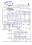
Table 4.2: Scores of every tool.
The reached results of the benchmark are placed in Table 4.2. In the table for every
tool there are six different properties scored, namely real-time, resources, Time To Product,
messages, costs and simulation. The scores per column are relative to each other. Real-time
indicates how easy the timing constraints are met. Resources indicates the used hardware
for the implementation. Time To Product (TTP) indicates the spent time to get a working
result. Messages indicates if the error and warning messages from the compiler are clear. Costs
indicates the license costs of the tool. Simulation indicates the effort to run a simulation.
Table 4.2 starts with the column real-time. Real-time is in our concept the most important
parameter. The solution is useless if it do not meet the timing constraints. All tools meet
the constraints. For CatapultC the designer has to increase the frequency. In Compaan
the timing can be easily improved by duplicating function calls. The resources used for the
implementation are almost the same for CatapultC and Compaan. The resources for ROCCC
are much more. The Time To Product (TTP) is for ROCCC very bad, it is hard to design
the code in the right way. The TTP of Compaan is in compare with CatapultC a bit longer.
The compiler warning and error messages of CatapultC are the most clear. For ROCCC
and Compaan the clearance of the messages is depending on the stage the problem is found.
In later stages ROCCC almost always outputted one common error message without a line
number. If the costs of the tools are compared CatapultC is by far the most expensive tool, the
open-source ROCCC tools is for free. All tools have there own innovative way of simulation
and validation, there is no big difference.
This benchmarking is done to select one tool to use for a case study. It is possible that a
person who is more familiar with one of the three tools, is able to get a higher performance
out of the tools. The assumption is done that the knowledge about these tools was good
enough to make a fair comparison. All tools are used for at least one month before scoring
the use case.
Finally, Compaan will be used because of the good average scores. CatapultC has got a
better score for some properties, but the difference is small. The biggest drawback of CatapultC are the extreme high annual costs. A cost-efficient solution is for
important.
Compaan is not a total solution, therefore some computational nodes have to be created
outside Compaan.
22
5
Implementation CONFIDENTIAL
5.1
5.2
5.3
5.4
5.5
5.6
5.7
23
5.8
Conclusion
In this Chapter the implementation of the mathematical model is described. Four keywords
(speed, optimization, hybrid and interleaving) are explained and discussed with examples
from the implementation.
speed The first example shows that Compaan is able to handle data flows with critical timing
constraints. Compaan is able to divide big shared memories in smaller distributed
memories with parallel processes. Parallelism can easily be increased by copying lines
multiple times, therefore high processing speeds can be realized.
optimization The second example shows a big memory optimization in comparison with the
implementation. In the
implementation data is stored redundantly, to
avoid complex reordering logic. Compaan is able to generate a FIFO construction for
the user to easily reorder data streams.
hybrid The third example shows how Compaan can be used in a hybrid construction. Compaan is not designed to generate the complete VHDL. The computational units should
be implemented outside Compaan. Three different approaches are used to implement a
computational unit, namely: manually (see Appendix B), CatapultC (see Appendix A.2)
or ROCCC. In general the three different approaches score the same.
interleaving The fourth example discussed the quality of Compaan to interleave data
streams. Streams can easily be interleaved and merged together. Therefore more parallelism and throughput can be achieved.
24
6
Results
In the previous chapter the implementation of several modules of the mathematical model
are described. In this chapter the total result is evaluated and discussed. The evaluation is
done by validating the output and timing performance. Finally some development ‘problems’
are discussed.
6.1
Output validation
To ensure a correct output of the system the total system is validated in four ways. (Most
of the validations are also done for intermediate results.) For every validation the test input
and output values are read from files. These files are generated with the mathematical model
of the system in Matlab. In this way input and output of both systems are always the same.
The input files contain 8160(=40x204) samples for each ADC, this number is equal to forty
runs of the total system. The four different validations are: data flow, RTL, after synthesis
and real-world.
data flow The first validation is done by compiling the Compaan source c-files with the GNU
Figure 6.1: Real-world output (metal object moved over the coils).
25
Compiler Collection (GCC) and by running the executable with input files. To achieve
this compiling two small GCC macros are written (to read the input stream and to check
the output stream). This validation is the most easy and fast way of validation. This
validation validates only the data flow of the system, timing and Compaan sub-blocks
are not tested. This validation is done to find main problems in the data flow.
RTL The second validation can be done after mapping the KPN to an XMP-file. The
generated XMP-file and the generated test bench file can be added to a Xilinx project
and the RTL behavior can be simulated in Simulink. The input and output files are
automatically read and processed. If the simulation results differ with output files an
ERROR flag is set. With this simulation timing constraints can also be validated. In
the test bench file a timeout value can be set to check if the whole system is ready
within the specified time. But if more exact time is required, manual measurement in
the wave files is necessary.
after synthesis The third validation can be done after synthesis the VHDL. Xilinx offers
the possibility to simulate intermediate results in the process to generate a binary for
the FPGA. The first simulation (behavioral[18]) is used to verify the RTL code and
to confirm that the design is functioning as intended (this is done in the previous
validation). The second simulation (post-translate[19]) verifies that design is correct
after the translation process. This simulation is primarily used in this validation, but
the simulations permanently failed to run. It is remarkable that basic designs do not
pass this Xilinx validation, too. Xilinx confirms this problem but doesn’t provide a
solution. Therefore another way to validate the design after synthesis is applied. This
validation is done by adding tables with static ADC samples to the design and by
running this modified design on the real-platform. The output received by the network
is compared with the proposed output.
real-world The fifth validation is the final validation. It is almost the same validation as the
previous one. Only this time with real ADC samples. A metal object is moved over the
coils and the results are interpreted for a natural result on the terminal. In Figure 6.1
the result is shown. A more detailed view of the picture shows the several coils reacting
after each other.
6.2
Timing performance
The timing constraints of the system are based on the maximum rotation speed of the roll
and the desired measurement precision. The data stream measured from the coils is 3.2 GBit
per second and a common measurement takes at least 3 minutes. In this case more than
500 TBits of data is gathered. Therefore it is not possible to store the measurement values
temporally to process it at a later moment. The implementation built with Compaan, is able
to process the data real-time.
Despite the fact that the system met the given timing constraints it is interesting to
know if the implementation is time optimal. To answer this question the correlation between
the estimated area and the number of cycles for the demodulation of one coil is calculated
and plotted in Figure 6.2. The plotted points (blue line with squares) in the graph are
calculated with the Scheduling Toolbox for MATLAB[1]. If the design is scheduled with
26
450
400
300
timing constraints
estimated area
350
250
200
150
100
50
(6,6)
(3,3)
(2,2)
(1,1)
Compaan
0
0
500
1000
1500
2000
2500
3000
3500
number of cycles
Figure 6.2: Demodulation performance for one ADC.
unlimited resources and the calculations are performed ‘as soon as possible (ASAP)’ nine
cycles are used (asymptote on the left of the figure). The maximal number of 3256 cycles
is found if all the instructions are executed in serial. The other points are calculated by
limiting the available resources. Four points are marked with the used resources (number of
MULTIPLIERs, number of ADDERs).
The Compaan implementation is also marked in the graph. The Compaan implementation
uses 2040 cycles to complete. Within the Compaan implementation one multiplier and one
adder is used. The result of the Scheduling Toolbox for one multiplier and one adder is ready
in 1697 cycles. The Scheduling Toolbox calculates a better result than Compaan because
it calculates the minimum number of calculations. Compaan calculates more to keep the
demodulation simple. The timing of the Compaan implementation is exact within the timing
constraints. If the demodulation runs faster the system will not improve. If the demodulation
will run slower the system will fail. So removing the useless calculations from Compaan will
not improve the quality but only increase complexity.
6.3
Comparison Simulink and Compaan implementation
As mentioned in the background (Section 3.2),
implements the model in Simulink. In
this section the Simulink implementation is compared against the Compaan implementation.
6.3.1
Timing
If the timing is compared, there is less difference, both implementations met the timing
constraints. Therefore it is not interesting to give a detailed comparison about timing. But
there is something to say about how the (timing) constraints are established. The global
timing constraints are based on the maximum allowed rotation speed of the roll, two meter
per second and are defined by the NDT-specialist. Based on this global constraints subconstraints are defined, for instance the speed of the filters which is 6,8kHz. Every filter
needs a coefficient table. The constraint of the coefficient table is unlike the filter timing
constraint not defined by the NDT-specialist but by the hardware engineer. The hardware
27
engineer defines the filter coefficient size at 1000 coefficients. 1000 is the maximal number
of serial instructions that can be executed within the given time (see Equation 6.1). In
the equation the maximum filter and system frequency is used, therefore the filter is very
area/time efficient. The Compaan design is running on 100MHz, so only 714 instructions can
be executed (see Equation 6.2). To execute the same number of instructions more parallelism
is necessary. Constraints optimizations like the filter coefficient size have been done more
often in the system.
systemf req
140MHz
max instructions =
max instructions =
6.3.2
f ilterf req
inputwidth
systemf req
f ilterf req
inputwidth
7kHz
=
20
=
100MHz
7kHz
20
= 1000
(6.1)
= 714
(6.2)
Resources
The used resources are compared for both implementations. Two parts from the mathematical
model are selected to be compared, namely: demodulation and one filter (see Figure 1.2). The
demodulation is implemented only once. The filter is implemented eight times. In Table 6.1
the used resources are displayed per part. These values are obtained from the ‘Module Level
Utilization report’ of Xilinx. Six categories are defined, namely: Slices, Slice Reg, LUTs,
LUTRAM, BRAM/FIFO and DSP48A1.
Slices
available
demodulation
- Simulink
- Compaan
filter
- Simulink
- Compaan
23038
Slice Reg
184304
LUTs
92152
LUTRAM
21680
BRAM/FIFO
268
DSP48A1
180
5490
6324
23,8%
27,5%
15684
7363
8,5%
4,0%
10609
10358
11,5%
11,2%
6034
1632
27,8%
7,5%
29
13
10,8%
4,9%
33
29
18,3%
16,1%
122
1616
0,5%
7,0%
206
2037
0,1%
1,1%
176
3073
0,2%
3,3%
67
219
0,3%
1,0%
5
15
1,9%
5,6%
1
2
0,6%
1,1%
Table 6.1: A comparison of the used resources of two parts.
The resources used for the demodulation implementation, differ per category. The small
differences are Slices, Slice Reg, LUTs and DSP48A1. The two main differences are LUTRAM
and BRAM/FIFO. More resources are used for Simulink, respectively 20% and 6%.
LUTRAM (+20%) For the Simulink implementation 20% more Look-Up Tables are used
as distributed RAM(LUTRAM). This difference is introduced by the calculation of
more than 200 moving averages. The Compaan implementation uses a FIFO to store
the values (see Section 5.4). The Simulink implementation uses Look-Up Tables to store
these values.
BRAM/FIFO (+6%) The Simulink implementation uses more BRAMs than the Compaan
implementation because it stores data redundantly (see Section 5.3).
The resources used for the filter differ per category not more than 6,5% in compare with
the total available resources. But the differences are scaled up with eight because the filter is
implemented eight times. The common reason why more resources are used is explained in
Section 6.3.1. Because of the used frequency of Compaan the implementation is conducted
28
twice and therefore it is less area efficient. The categories Slices(-6,5%) and BRAM/FIFO’s(3,7%) form the main differences.
Slices(-6,5%) The difference in Slices is because Compaan implements the filter in fifteen
nodes. (Fifteen nodes are relatively many nodes.) Every node has its own switching
logic.
BRAM/FIFO’s(-3,7%) Bigger FIFO’s and BRAM’s are used to store the intermediate
results in Compaan. Because Compaan can only handle FIFO’s with a bit-width of
8,16,32,64. With Simulink it is possible to apply bit-with narrowing. For instance the
DSP of the filter. The original bit-with of the DSP-output is 48bits. The 48bits are
stored in a 64bit width FIFO. This is (64 − 48) ∗ 1000 = 16000bits wasted space.
6.3.3
Power consumption
The power consumption is not a main issue in the implementation. But if the power consumption is compared, the power consumption of the Compaan implementation is 100mA
less. There are some possible factors that contribute to this power reduction.
• The clock speed of the Compaan system is lower (140MHz versus 100MHz).
• The Compaan implementation uses half of the BRAMs of the Simulink implementation.
• The wrappers (used to read the BRAMs) are disabling the BRAMs when they are not
used.
6.4
Development problems with Compaan
In this section some development problems achieved with Compaan are listed. Note that the
implementation is done with the ‘nice alpha 2011’ version of Compaan. This version can be
used for production purposes but is still under active development. This list of problems is
already reported and probably fixed in the next release. For all the problems below there is
a (suboptimal) workaround.
• RTL level simulation of hierarchical designs is not possible. To keep the Compaan models more readable, it is possible to create designs with hierarchy. Simulating
the total hierarchical design at RTL level is not possible. It is only possible to simulate
the sub-levels independent of each other.
• Some times the KPN-rate-matcher fails. As explained in Section 5.3, some times
the KPN-rate-matcher failed to calculate the most optimal size of the FIFO’s. Therefore
manually changes are preferred. Note that there is a message to warn the user most of
the time.
• The absence to run code only once for initialization. In the Compaan implementation several times a self-loop is used for node. The self-loops are used to store
intermediate results, (for instance at the moving average in Section 5.4). At the initialization (only once), these self-loops have to be initialized with zeros. In Compaan it is
not possible to execute code only once. Therefore a simple patch is built in the current
implementation. This patch defines an initialization signal and changes the switching
logic of the node a little bit.
29
• Only restricted bit-widths possible. The size of the FIFO’s within Compaan are
limited to a bit-width of: 8, 16, 32 or 64. Often these widths are not optimal sizes and
so resources are wasted for too big FIFO’s (see Section 6.3.2).
• More nodes are used than strictly necessarily. The final implementation calculated by Compaan is sometimes suboptimal. Some nodes can be removed without
breaking down the system (see Section 5.3). Note that Compaan already designed an
algorithm to find these useless nodes. In a future release the nodes will be removed.
• No loop unrolling parameter. Especially in the demodulation there is much parallelism. In Compaan there is no parameter to unroll loops, therefore some lines of code
are duplicated twenty-four times.
30
7
Conclusion /
Recommendations
During this thesis the mathematical model of the
inspection system is implemented
in hardware. In preparation of this implementation three High-Level Synthesis (HSL) tools
are benchmarked. Before benchmarking these tools were explored during one month. A short
summery of the tools below:
CatpultC is a professional and versatile HLS tool. This non-visual HLS tool uses ANSI C as
input. The CatapultC compiler is highly configurable and the Graphical User Interface
(GUI) is easy to use. More parallelism can be introduced by unrolling loops. To be able
to create parallelism, shared memory should be avoid in the ANSI C file (or mapped to
registers). The high annual cost is the main drawback of this tool.
ROCCC 2.0 is an open source HLS tool which accepts a subset of the C-programming
language and is freely available. The small list of coding limitations (included in the
manual) makes it hard to design a complex system. Many skills are necessary to create
bigger systems and models in ROCCC. ROCCC is still under development.
Compaan is a powerful tool designed to handle data streams with high timing constraints.
Like the other tools the input of Compaan is an ANSI C file. The power of Compaan
is the capability to change shared memories (used in the source code) into distributed
memories with concurrent processes. Compaan generates not a full solution. Computational nodes have to be created outside Compaan.
After the benchmark Compaan is chosen to implement the mathematical model. The
benchmarking shows that Compaan is able to implement complex systems in a short time.
More parallelism can be created by duplicating the function calls of the computational units.
Shared memories are automatically split into distributed memories. Distributed memories
provide the input data of the computational units without interference. The learning curve
to use Compaan is steep, the designer should learn to think in the Compaan approach of
‘nodes’ and ‘edges’.
In Compaan the implementation of the mathematical model is done in four months.
This is approximately four times faster than the implementation with Simulink. Also
future maintenance of the Compaan implementation will be faster because the Compaan
implementation is of a higher abstraction. Critical analyze of the Simulink implementation
confirms that detailed knowledge about the system is required to design and maintain the
Simulink implementation. For instance: some implementation related questions were hard to
answer for the hardware engineer even a few months after implementation.
Using Compaan in a hybrid construction will give efficient results. A second tool to
generated the computation nodes is desirable. Although a hardware engineer with average
VHDL scales will be able to create most of the computational nodes manually by using the
31
pipeline templates. The user should keep the computational nodes as simple as possible, by
moving logic to Compaan as much as possible.
The resources used for the whole implementation in Compaan are approximately 15%
higher than the resources used in the Simulink implementation. Compaan is under active
development and improves. Although Compaan is still in an alpha version the tool is very
useful. Using Compaan is recommended for the implementation of systems with a complex
data-flow in both small and medium-sized enterprises.
7.1
future work
Many design optimizations related to more parallelism can be easily applied by using Compaan. Below a list of optimisations. (Note if these optimisations are applied with Simulink
implementation would take much more time.)
• Increase sample speed to handle higher rotation speed of the roll.
• Use more coils to increase scan speed.
• Increase filter coefficients to improve filtering.
• Lower clock speed to decrease power.
Finally, the interfacing between the already designed network of
and the Compaan
system gave the most problems during the first implementation state of the system. However
Compaan provides board templates. In these board templates the network interface is already
designed. In future designs such a board template could be very useful.
32
Bibliography
[1] Ing. H.J. Lincklaen Arrins, Scheduling Toolbox for MATLAB, http: // ens. ewi.
tudelft. nl/ Education/ courses/ et4054/ Lab2011/ msclab2008_ RG. pdf , 2008.
[2] Semiconductor Industry Association., The International Technology Roadmap for Semiconductors, (2009), 10.
[3] Compaan Design, heterogeneous compilation, http://www.compaandesign.com/.
[4] Eclipse, IDE for C/C++ Developers, http://www.eclipse.org/downloads.
[5] Mentor Graphics, Catapult C Synthesis, http://www.mentor.com/esl/catapult/.
[6]
, Communities, http://communities.mentor.com/.
[7] Jacquard Computing inc, Riverside Optimizing Compiler for Configurable Computing,
http://www.jacquardcomputing.com/roccc/.
[8]
, ROCCC 2.0 User’s Manual - Revision 0.6, feb. 2011.
[9] National Instruments, The Benefits of Programming Graphically in NI LabVIEW, http:
//www.ni.com/labview/whatis/graphical-programming/.
[10] A. Madariaga, J. Jime andnez, J.L. Marti andn, U. Bidarte, and A. Zuloaga, Review
of electronic design automation tools for high-level synthesis, Applied Electronics (AE),
2010 International Conference on, sept. 2010, pp. 1–6.
®
[11] MathWorks , MATLAB - The Language Of Technical Computing, http://www.
mathworks.nl/products/matlab/.
[12]
, Simulink - Simulation and Model-Based Design, http://www.mathworks.nl/
products/simulink.
[13]
, Using Simulink with Xilinx System Generator for DSP, http://www.
mathworks.nl/fpga-design/simulink-with-xilinx-system-generator-for-dsp.
html.
[14] Gordon E. Moore, Cramming more components onto integrated circuits, reprinted from
electronics, volume 38, number 8, april 19, 1965, pp.114 ff., Solid-State Circuits Newsletter, IEEE 20 (2006), no. 3, 33 –35.
[15] NDT resource center, Introduction to Eddy Current Testing, http://www.ndt-ed.org/
EducationResources/CommunityCollege/EddyCurrents/cc_ec_index.htm.
[16] Patrick Schaumont, Doris Ching, and Verbauwhede Ingrid, An interactive codesign environment for domain-specific coprocessors, jan. 2006.
[17] T. Stefanov, C. Zissulescu, A. Turjan, B. Kienhuis, and E. Deprette, System design using
khan process networks: the compaan/laura approach, Design, Automation and Test in
Europe Conference and Exhibition, 2004. Proceedings, vol. 1, feb. 2004, pp. 340 – 345
Vol.1.
33
®
[18] Xilinx , Performing Behavioral Simulation, http://www.xilinx.com/itp/xilinx10/
isehelp/pp_p_process_simulate_behavioral_model.htm.
[19]
, Performing Post-Translate Simulation, http://www.xilinx.com/itp/
xilinx10/isehelp/pp_p_process_simulate_post_translate_model.htm, 2008.
®, FPGAs, http://www.xilinx.com/products/silicon-devices/fpga.
[20] Xilinx
34
CatapultC design notes
A
This appendix contains two design notes for the use of CatapultC. The first note describes
the problem of synthesizing CatapultC code with the Xilinx XST synthesizer. The second
note describes how a Compaan computational node can be created with CatapultC.
A.1
Xilinx XST synthesis tool
No official messages can be found about the CatapultC compiler support. At the start of the
project several times the Xilinx XST synthesizer was used to compile the CatapultC results.
It was very confusing that the results didn’t work properly. Searching on internet the Mentor
Community[6] was found. Posts of the mentor community mentioned several times that the
Xilinx XST synthesizer is not supported.
In practise simple models can be synthesized without warnings and errors. But the synthesized models are not correct, sometimes. For example: Block RAMs are implemented with
LUTs and the timing constraints do not meet.
A.2
Create node for Compaan
Compaan supports the possibility to link CatapultC computational nodes. If the correct steps
are done, linking is very easy and exists of four steps.
First the CatapultC module should be referenced in the Compaan C-code. In Listing A.1
there is an example of the computational node MAC with three inputs (sample, coef, sum)
and one output (result). The first pragma(line 1) in the listing specifies that the function is
implemented in CatapultC. The second pragma(line 2) is optional and specifies that the function
is provided as EDIF-file1 . It is also possible to remove this pragma and provide a VHDLfile, but this is not recommended (for more details see Section A.1). Note that it is not
strictly necessary to specify the function contents in Compaan, but it can be used for C-code
simulations and it increases the readability of the code.
1
2
3
4
#pragma c o m p a a n_ p r o p e r t y mapto catapultc /* first pragma */
#pragma c o m p a a n_ p r o p e r t y netlist edf
/* second pragma (optional) */
v o i d MAC ( s h o r t sample , s h o r t coef , i n t sum , i n t * result )
{ * result = sum + ( sample * coef ) ; }
/* not strictly necessary */
Listing A.1: CatapultC reverence in Compaan
1
EDIF (Electronic Design Interchange Format) is a vendor-neutral format in which Electronic netlists and
schematics are stored
35
Secondly a new CatapultC project must Output
be created. It is very important to set a
[ v ] VHDL
[ v ] Package Output in Solution dir
number of global settings. Open the setFlows
tings window by menu ‘Tools’→‘Set OpPrecision RTL
[ ] Add IO Pads
tions...’ and apply the values listed in Listing A.2. Add a C-file to the project with
Listing A.2: CatapultC Options
the content of Listing A.3. Go to ‘Architecture Constraint’ and change the ‘Resource
Types’ of the input interfaces to ‘mgc ioport.mgc in wire wait’ and the ‘Resource Types’ of
the output interfaces to ‘mgc ioport.mgc out buf wait’. Thirdly generate the RTL and synthesize the design with Precision.
1
2
3
4
5
6
#include <ac_channel . h>
v o i d MAC ( ac_channel<s h o r t > &sample , ac_channel<s h o r t > &coef ,
ac_channel<i n t > &sum ,
ac_channel<i n t > &result )
{
result . write ( sum . read ( ) + sample . read ( ) * coef . read ( ) ) ;
}
Listing A.3: CatapultC computational node
Finally copy the EDIF-file (e.g. psr vhdl impl/MAC.edf) to Compaan (e.g. projectname KpnMapper 1/pcores/Functions v1 00 a/netlist/MAC.edf). Note if the second
pragma(line 2) in Compaan is removed then copy the VHDL-file (e.g. concat MAC.vhdl) to
Compaan (e.g. projectname KpnMapper 1/pcores/Functions v1 00 a/hdl/vhdl/MAC.vhd).
36
B
Compaan pipeline
Compaan is able to generate a pipeline template. Two parts of code must be added to generate
a template(see Figure B.1). First a pragma(line 1) must be added and after that a C-function
description(line 4-6). The generated pipeline template is displayed below Figure B.1.
1
2
3
4
#pragma c o m p a a n_ p r o p e r t y pipeline 3
v o i d combi ( i n t intermidate_in ,
i n t sum_in ,
i n t sum_last10_in ,
i n t offset_gain_in ,
i n t * sum_last10_out , i n t * intermidate_out , i n t
*
ans_out ) { }
Figure B.1: Source to generate a pipeline template in Compaan.
1
2
3
−− F i l e a u t o m a t i c a l l y g e n e r a t e d by KpnMapper
−− This f i l e d e f i n e s a t e m p l a t e f o r p i p e l i n e d f u n c t i o n i m p l e m e n t a t i o n
−− F u n c t i o n ” p r o j e c t i o n c o m b i ”
4
5
6
7
l i b r a r y ieee ;
u s e ieee . std_ logic_11 64 . a l l ;
u s e ieee . numeric_std . a l l ;
8
9
10
l i b r a r y comm on_v1_00 _a ;
u s e commo n_v1_00 _a . hw_node_pkg . a l l ;
11
12
13
14
15
16
17
18
19
20
21
22
23
24
25
26
27
28
29
30
31
32
33
34
35
36
37
38
39
40
e n t i t y projection_combi_pipeline i s
generic (
c_STAGES
: natural := 1 ;
N_CNTRS
: natural := 1 ;
CNTR_QUANT : natural := 3 2 ;
CNTR_WIDTH : t _c ou nt e r_ wi dt h := ( 0=>10, 1=>10, 2=>9, o t h e r s =>10 )
);
port (
RST
: in
std_logic ;
CLK
: in
std_logic ;
−− I n p u t s
ip_intermidate_in
: in
s t d _ l o g i c _ v e c t or ( 3 1 downto 0 ) ;
ip_sum_in
: in
s t d _ l o g i c _ v e ct o r ( 3 1 downto 0 ) ;
i p _ s u m _ l a s t 1 0_ i n
: in
s t d _ l o g i c _ v e c t or ( 3 1 downto 0 ) ;
ip_offset_gain_in
: in
s t d _ l o g i c _ v e c t or ( 3 1 downto 0 ) ;
−− I t e r a t o r s
it_index : i n
s t d _ l o g i c _ v e c t o r ( CNTR_WIDTH ( 0 )−1 downto 0 ) ;
it_set : i n
s t d _ l o g i c _ v e c t o r ( CNTR_WIDTH ( 1 )−1 downto 0 ) ;
it_i : i n
s t d _ l o g i c _ v e c t o r ( CNTR_WIDTH ( 2 )−1 downto 0 ) ;
−− Outputs
o p _ s u m _ l a s t 1 0 _ o u t : out s t d _ l o g i c _ v e c t or ( 3 1 downto 0 ) ;
o p _ i n t e r m i d a t e _ o u t : out s t d _ l o g i c _ v e c t or ( 3 1 downto 0 ) ;
op_ans_out : out s t d _ l o g i c _ v e c t o r ( 3 1 downto 0 ) ;
−−
ENi
: in
std_logic ;
EN
: in
s t d _ l o g i c _ v e c t o r ( c_STAGES −1 downto 0 ) ;
STALL_FRONT
: out s t d _ l o g i c _ v e c to r ( c_STAGES −1 downto 0 ) ;
STALL_BACK
: out s t d _ l o g i c _ v e c to r ( c_STAGES −1 downto 0 ) ;
ERROR : out std_logic
37
41
42
);
end p r o j e c t i o n _ c o m b i _ p i p e l i n e ;
43
44
45
46
47
48
49
50
51
52
53
54
55
56
57
58
59
60
61
62
63
64
65
66
67
68
69
70
71
72
73
74
75
76
77
78
79
80
81
82
83
84
85
86
87
88
89
90
91
92
93
94
95
96
97
98
99
100
101
102
103
104
105
106
a r c h i t e c t u r e RTL o f p r o j e c t i o n _ c o m b i _ p i p e l i n e i s
c o n s t a n t error_int : integer := −1;
c o n s t a n t reset_int : s t d _ l o g i c _ v e c to r ( 0 downto 0 ) := b ” 0 ” ;
−− I n p u t r e g i s t e r s
s i g n a l i p r _ i n t e r m i d a t e _ i n : s t d _ l o g i c _ v e c t or ( 3 1 downto 0 ) ;
s i g n a l ipr_sum_in : s t d _ l o g i c _ v e c to r ( 3 1 downto 0 ) ;
s i g n a l i p r _ s u m _ l a s t 1 0 _ i n : s t d _ l o g i c _ v e c t or ( 3 1 downto 0 ) ;
s i g n a l i p r _ o f f s e t _ g a i n _ i n : s t d _ l o g i c _ v e c t or ( 3 1 downto 0 ) ;
−− I t e r a t o r r e g i s t e r s
s i g n a l itr_index : s t d _ l o g i c _ v e ct o r ( CNTR_WIDTH ( 0 )−1 downto 0 ) ;
s i g n a l itr_set : s t d _ l o g i c _ v e c t o r ( CNTR_WIDTH ( 1 )−1 downto 0 ) ;
s i g n a l itr_i : s t d _ l o g i c _ v e c t o r ( CNTR_WIDTH ( 2 )−1 downto 0 ) ;
−−
−− Your p i p e l i n e s i g n a l s
−− STAGE 0
s i g n a l s 0 _ i n t e r m i d a t e _ i n : s t d _ l o g i c _ v e c t or ( 3 1 downto 0 ) ;
s i g n a l r 0 _ i n t e r m i d a t e _ i n : s t d _ l o g i c _ v e c t or ( 3 1 downto 0 ) ;
s i g n a l s0_sum_in : s t d _ l o g i c _ v e ct o r ( 3 1 downto 0 ) ;
s i g n a l r0_sum_in : s t d _ l o g i c _ v e ct o r ( 3 1 downto 0 ) ;
s i g n a l s 0 _ s u m _ l a s t 1 0 _i n : s t d _ l o g i c _ v e c t or ( 3 1 downto 0 ) ;
s i g n a l r 0 _ s u m _ l a s t 1 0 _i n : s t d _ l o g i c _ v e c t or ( 3 1 downto 0 ) ;
s i g n a l s 0 _ o f f s e t _ g a i n _ i n : s t d _ l o g i c _ v e c t or ( 3 1 downto 0 ) ;
s i g n a l r 0 _ o f f s e t _ g a i n _ i n : s t d _ l o g i c _ v e c t or ( 3 1 downto 0 ) ;
−− STAGE 1
s i g n a l s 1 _ i n t e r m i d a t e _ i n : s t d _ l o g i c _ v e c t or ( 3 1 downto 0 ) ;
s i g n a l r 1 _ i n t e r m i d a t e _ i n : s t d _ l o g i c _ v e c t or ( 3 1 downto 0 ) ;
s i g n a l s1_sum_in : s t d _ l o g i c _ v e ct o r ( 3 1 downto 0 ) ;
s i g n a l r1_sum_in : s t d _ l o g i c _ v e ct o r ( 3 1 downto 0 ) ;
s i g n a l s 1 _ s u m _ l a s t 1 0 _i n : s t d _ l o g i c _ v e c t or ( 3 1 downto 0 ) ;
s i g n a l r 1 _ s u m _ l a s t 1 0 _i n : s t d _ l o g i c _ v e c t or ( 3 1 downto 0 ) ;
s i g n a l s 1 _ o f f s e t _ g a i n _ i n : s t d _ l o g i c _ v e c t or ( 3 1 downto 0 ) ;
s i g n a l r 1 _ o f f s e t _ g a i n _ i n : s t d _ l o g i c _ v e c t or ( 3 1 downto 0 ) ;
−− STAGE 2
s i g n a l s 2 _ i n t e r m i d a t e _ i n : s t d _ l o g i c _ v e c t or ( 3 1 downto 0 ) ;
s i g n a l r 2 _ i n t e r m i d a t e _ i n : s t d _ l o g i c _ v e c t or ( 3 1 downto 0 ) ;
s i g n a l s2_sum_in : s t d _ l o g i c _ v e ct o r ( 3 1 downto 0 ) ;
s i g n a l r2_sum_in : s t d _ l o g i c _ v e ct o r ( 3 1 downto 0 ) ;
s i g n a l s 2 _ s u m _ l a s t 1 0 _i n : s t d _ l o g i c _ v e c t or ( 3 1 downto 0 ) ;
s i g n a l r 2 _ s u m _ l a s t 1 0 _i n : s t d _ l o g i c _ v e c t or ( 3 1 downto 0 ) ;
s i g n a l s 2 _ o f f s e t _ g a i n _ i n : s t d _ l o g i c _ v e c t or ( 3 1 downto 0 ) ;
s i g n a l r 2 _ o f f s e t _ g a i n _ i n : s t d _ l o g i c _ v e c t or ( 3 1 downto 0 ) ;
begin
PIPE_REGS : p r o c e s s ( CLK )
begin
i f rising_edge ( CLK ) then
i f ( RST = ' 1 ' ) then
−− Something t o r e s e t ?
else
i f ( ENi = ' 1 ' ) then
−− I n p u t R e g i s t e r s
i p r _ i n t e r m i d a t e _ i n <= i p _ i n t e r m i d a t e _ i n ;
ipr_sum_in <= ip_sum_in ;
i p r _ s u m _ l a s t 1 0 _ i n <= i p _ s u m _ l a s t 1 0 _i n ;
i p r _ o f f s e t _ g a i n _ i n <= i p _ o f f s e t _ g a i n _ i n ;
−− I t e r a t o r R e g i s t e r s
itr_index <= it_index ;
itr_set <= it_set ;
itr_i <= it_i ;
end i f ;
−− P i p e l i n e Depth : 3 s t a g e s
−− STAGE 0
i f ( EN ( 0 ) = ' 1 ' ) then
r 0 _ i n t e r m i d a t e _ i n <= s 0 _ i n t e r m i d a t e _ i n ;
38
107
108
109
110
111
112
113
114
115
116
117
118
119
120
121
122
123
124
125
126
127
128
129
130
131
132
133
134
135
136
137
138
139
140
141
142
143
144
145
146
147
148
149
r0_sum_in <= s0_sum_in ;
r 0 _ s u m _ l a s t 1 0 _ i n <= s 0 _ s u m _ l a s t 1 0_ i n ;
r 0 _ o f f s e t _ g a i n _ i n <= s 0 _ o f f s e t _ g a i n _ i n ;
end i f ;
−− STAGE 1
i f ( EN ( 1 ) = ' 1 ' ) then
r 1 _ i n t e r m i d a t e _ i n <= s 1 _ i n t e r m i d a t e _ i n ;
r1_sum_in <= s1_sum_in ;
r 1 _ s u m _ l a s t 1 0 _ i n <= s 1 _ s u m _ l a s t 1 0_ i n ;
r 1 _ o f f s e t _ g a i n _ i n <= s 1 _ o f f s e t _ g a i n _ i n ;
end i f ;
−− STAGE 2
i f ( EN ( 2 ) = ' 1 ' ) then
r 2 _ i n t e r m i d a t e _ i n <= s 2 _ i n t e r m i d a t e _ i n ;
r2_sum_in <= s2_sum_in ;
r 2 _ s u m _ l a s t 1 0 _ i n <= s 2 _ s u m _ l a s t 1 0_ i n ;
r 2 _ o f f s e t _ g a i n _ i n <= s 2 _ o f f s e t _ g a i n _ i n ;
end i f ;
end i f ;
end i f ;
end p r o c e s s ;
−− PIPE REGS
−− Output
o p _ s u m _ l a s t 1 0 _ o u t <= S T D _ L O G I C _ V E C TO R ( RESIZE ( UNSIGNED ( r 2 _ i n t e r m i d a t e _ i n ) , ←op_sum_last10_out ' Length ) ) ;
o p _ i n t e r m i d a t e _ o u t <= S T D _ L O G I C _ V E C TO R ( RESIZE ( UNSIGNED ( r2_sum_in ) , ←op_intermidate_out ' Length ) ) ;
op_ans_out <= S T D _ L O G I C _ V E C T O R ( RESIZE ( UNSIGNED ( r 2 _ s u m _ l a s t 1 0 _ i n ) , op_ans_out ' ←Length ) ) ;
−− PIPE COMB :
s 0 _ i n t e r m i d a t e _ i n <= i p r _ i n t e r m i d a t e _ i n ;
s0_sum_in <= ipr_sum_in ;
s 0 _ s u m _ l a s t 1 0 _ i n <= i p r _ s u m _ l a s t 1 0 _ i n ;
s 0 _ o f f s e t _ g a i n _ i n <= i p r _ o f f s e t _ g a i n _ i n ;
s 1 _ i n t e r m i d a t e _ i n <= r 0 _ i n t e r m i d a t e _ i n ;
s1_sum_in <= r0_sum_in ;
s 1 _ s u m _ l a s t 1 0 _ i n <= r 0 _ s u m _ l a s t 1 0 _i n ;
s 1 _ o f f s e t _ g a i n _ i n <= r 0 _ o f f s e t _ g a i n _ i n ;
s 2 _ i n t e r m i d a t e _ i n <= r 1 _ i n t e r m i d a t e _ i n ;
s2_sum_in <= r1_sum_in ;
s 2 _ s u m _ l a s t 1 0 _ i n <= r 1 _ s u m _ l a s t 1 0 _i n ;
s 2 _ o f f s e t _ g a i n _ i n <= r 1 _ o f f s e t _ g a i n _ i n ;
−−
STALL_FRONT <= ( o t h e r s = > ' 0 ' ) ;
STALL_BACK
<= ( o t h e r s = > ' 0 ' ) ;
ERROR <= ' 0 ' ;
end RTL ;
39
40
Eddy Current response graphs
- CONFIDENTIAL
C.1
41
C