Download ANAT: a Tool for Constructing and Analyzing

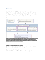
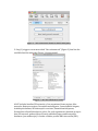
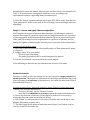
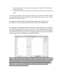
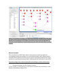
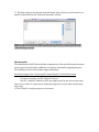
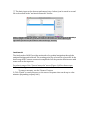
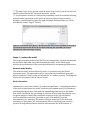
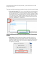
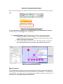
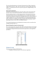
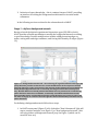
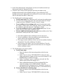
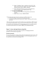
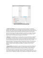
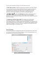
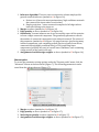
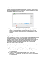
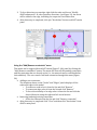
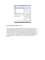
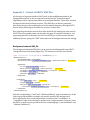
ANAT: a Tool for Constructing and Analyzing Functional Protein Networks User Manual Contents Introduction.................................................................................................................3 Installation...................................................................................................................3 Pre­requisites .............................................................................................................................................................. 3 Installation ................................................................................................................................................................... 4 Starting and saving work sessions ..................................................................................................................... 4 Basic usage ..................................................................................................................5 Stage 1 – define a background network ...........................................................................................................5 Stage 2 – choose and apply inference algorithm ..........................................................................................7 Anchored networks ................................................................................................................................................... 7 General networks....................................................................................................................................................... 9 Shortest paths ...........................................................................................................................................................10 Local search ...............................................................................................................................................................11 Stage 3 – explore the model................................................................................................................................12 Network model display .........................................................................................................................................12 Node information ....................................................................................................................................................12 Edge information.....................................................................................................................................................14 Sub­network information ....................................................................................................................................15 General information about the inference task............................................................................................15 Advanced usage .........................................................................................................15 Stage 1 – define a background network ........................................................................................................16 Stage 2 – choose and apply inference algorithm .......................................................................................18 Anchored networks .................................................................................................................................................18 General networks.....................................................................................................................................................20 Shortest paths ...........................................................................................................................................................21 Local search ...............................................................................................................................................................22 Stage 3 – refine the model ...................................................................................................................................22 Using the “Add/Remove constraints” menu.................................................................................................23 Using the “Modify parameters” option...........................................................................................................24 Appendix 1 – format of ANAT’s XML files ...................................................................25 Background network XML file...........................................................................................................................25 Query input XML files............................................................................................................................................26 Anchored networks .................................................................................................................................................26 General networks and local search..................................................................................................................26 Shortest paths ...........................................................................................................................................................27 Added constraints XML files...............................................................................................................................27 Introduction Genome‐scale screening studies are gradually accumulating a wealth of data on the putative involvement of hundreds of genes in various cellular responses or functions. A fundamental challenge is to chart out the molecular pathways that underlie these systems. ANAT (Advanced Network Analysis Tool), is an all‐in‐one resource that provides access to up‐to‐date large‐scale physical association data in several organisms, advanced algorithms for network reconstruction, and a plethora of tools for exploring and evaluating the obtained network models Strictly speaking, the output of ANAT is a high confidence protein network that links together (through protein‐protein interactions or protein‐dna interactions) an input set of proteins (not necessarily directly). It supports four types of network‐based analyses: (i) inferring an anchored network that connects a given set of proteins to a designated anchor set of proteins; (ii) inferring a non‐anchored network that connects a given set of proteins to each other; and (iii) viewing the local neighborhood of a given set of proteins, and (iv) finding the highest confidence paths between pairs of proteins ANAT is implemented in a client‐server architecture. The client side is implemented as a plugin to the Cytoscape platform. The server side contains a data repository of molecular interactions and protein annotations, and the network inference algorithmic engine. Installation Pre‐requisites 1. OS: Mac, windows or linux 2. Internet connection (ANAT is a client application and operates by connecting to an external server) 3. Java Runtime environment (version 6 and above) a. For Mac OSX10.5 users with a lower java version see: i. Updating your java version to 1.6 (http://support.apple.com/kb/HT3649) ii. Switching you default java version (http://blogs.sun.com/cmar/entry/java_1_6_finally_available) b. For Mac OSX10.4/5 users with a lower java version: i. Install SoyLatte java 6 for Mac (http://blog.adsdevshop.com/2008/02/26/installing‐the‐jdk‐
16‐on‐mac‐os‐x/) ii. Update your path variable: 1. open /Applications/Utilities/X11.app and type: export PATH=<bin directory of SoyLatte>:$PATH export DISPLAY=:0.0 4. Cytoscape version 2.7 (can download from : http://www.cytoscape.org/) Installation 1. Download ANAT Cytoscape plugin (http://www.cs.tau.ac.il/~bnet/ANAT_SI/Advanced%20Network%20Analysis%20Tool_files/AnatPlugin.jar) 2. Place the downloaded file in the "plugins" folder under your local Cytoscape folder. Starting and saving work sessions 1. To start ANAT simply start Cytoscape. The main menu of ANAT will appear as a separate tab on Cytoscape’s control pane. 2. To save a session use the “Save” option in Cytoscape. This will also save all the information in ANAT (modified background networks, input queries, reconstructed network models etc.). 3. All the types of input provided to ANAT can be exported and saved as specialized XML files. These files can then be imported and used in future sessions. The XML files can also be generated directly by the user, thus avoiding the need for manual data entry through ANAT’s menus. See Appendix 1 for description of file formats. Basic usage A typical workflow in ANAT (Figure 1) consists of three steps: (i) defining a background network; (ii) submitting a query for extracting a network model from the background network; and (iii) analyzing and refining the obtained network model. In the following we describe these step under a basic usage scenario that does not include addition of expert knowledge or adjustment of the default parameters. Figure 1: Given a set of genes, the construction of a network of physical associations that links these genes consists of three steps: (i) Adding prior knowledge (defining a background network); (ii) choosing the appropriate inference method and adjusting its parameters; and (iii) exploring the obtained model and refining it. Stage 1 – define a background network The first stage of the analysis is to define a background network from which the final sub‐network model will be extracted. Here are the steps for defining a background network: 1. Go to ANAT’s tab and click the “new subnetwork” button (Figure 2) Figure 2 – “New subnetwork” button in ANAT’s main panel 2. Step (1) triggers a new menu titled “New subnetwork” (Figure 3) that lists the available baseline networks (Figure 3; bottom panel). Figure 3 – the “New subnetwork” menu ANAT includes baseline PPI networks of ten organisms: Homo sapiens, Mus musculus, Rattus norvegicus, Drosophila melanogaster, Caenorhabditis elegans, Arabidopsis thaliana, Saccharomyces cerevisiae, Plasmodium falciparum, Escherichia coli and Helicobacter pylori. For each organism we obtained an up‐to‐
date PPI network, gathered from recently published papers and from public databases (see manuscript). It further contains protein‐DNA interaction (PDI) information for yeast and human. Network sizes and data sources are detailed in SI Table 1. All interactions are assigned a confidence score according to the experimental evidence supporting them (see manuscript). 3. Select the desired organism and interaction type (PPI, PDI or both). Note that the “New subnetwork” menu is also used on the next stage (choose and apply inference algorithm). Stage 2 – choose and apply inference algorithm ANAT supports four types of network‐based analyses: (i) inferring an anchored network that connects a given set of proteins to a designated anchor set of proteins; (ii) inferring a non‐anchored network that connects a given set of proteins to each other; and (iii) viewing the local neighborhood of a given set of proteins, and (iv) finding the highest confidence paths between pairs of proteins Anchored networks. To proceed, follow these steps: 1. Select one of the four inference tasks (middle panel on “New subnetwork” menu; see Figure 3). 2. Assign a name/ ID to your model. This step is not mandatory The name (if provided) will be used throughout the analysis 3. Click the “Next button” to proceed with the actual analysis In the following we describe the specialized menus for each of the tasks. Anchored networks The input to ANAT in this case consists of two sets of proteins: target proteins and anchor proteins. The output is a subnetwork of the background network that leads from each target to at least one of the anchors or vice versa (the direction of flow is determined by the user). For a basic usage of the “Anchored networks” menu (Figure 4) follow these steps: 1. Enter a list of targets and anchors. To remove an entry, use the “Remove” button. Note that there should be no overlap between the targets and anchors sets 2. Choose the direction of inference (from targets to anchors or vice versa) by setting the direction of the arrow between the sets 3. Click “Finish” to send you query to the server. Response time can be up to a few minutes (depending on query size) *** The basic input to the anchored networks menu (steps 1 and 2 above) can be saved to an xml file for future use: 1. To save the anchors/ targets/ direction input click “Export” and choose file location and name 2. To upload previously saved input click “Import” and choose file location and name ** Note that the export option provides another way to input data to ANAT. Instead of entering the proteins manually (one by one) to the menu, one can create an xml file and use the import option. An example xml file (defining the apoptosis‐autophagy input in Figure 4) is provided as part of the Supporting Information of the paper (input.xml). An example for an anchored network construction is given in Figure 4. The targets are authophagic genes and the anchor is Caspase3 – the main apoptosis executioner (note that in principle there can be more than one anchor protein). The resulting crosstalk network, aiming to capture the signaling‐regulatory events that lead from the autophagic genes to Caspase3, is depicted in Figure 5. Figure 4 ­ Anchored network menu (basic) – the primary inputs for this menu are two sets – a target set (left) and an anchor set (right); the output is a network that connects each target to at least one of the anchors. The arrow between the sets represent the direction of inference (from targets to anchors or vice versa). To construct the autophagy­apoptosis crosstalk network we entered a list of autophagic genes as targets and Caspase3, the main apoptosis executioner, as a sole anchor. The menu also allows adjusting the tool's parameters (described in “Advanced usage” Section). Figure 5 ­ the ahtophagy­apoptosis cross talk network. The network model is depicted within the main screen of Cytoscape with ANAT panels and information on the left and at the bottom. Members of the autophagic core­machinery, provided as a target set for the algorithm, are colored in red. The apoptosis executioner Caspase3, given as the sole anchor node, is colored in green. General networks The second mode of ANAT deals with reconstruction scenarios in which the investigated system is not known to be centralized around a well‐defined anchor. Instead, ANAT models the architecture of physical associations between the target proteins by searching the most probable subnetwork that links them to each other. For a basic usage of the “General networks” menu (Figure 6) follow these steps: 1. Enter a list of genes to be connected. To remove an entry, use the “Remove” button. 2. Click “Finish” to send you query to the server. Response time can be up to a few minutes (depending on query size) *** The basic input to the general networks menu (step 1 above) can be saved to an xml file as described in the “anchored networks” section. Figure 6 ­ General network menu (basic) – the input for this menu is a set of proteins to be linked together. The menu also allows adjusting the algorithm’s parameters (described in “Advanced usage” Section). Shortest paths The third mode of ANAT deals with the computation of the most likely path between a given pair of proteins (the confidence of a path is computed by aggregating over the confidence levels of its member edges and nodes). For a basic usage of the “shortest path” menu (Figure 7) follow these steps: 1. Enter a list of sources and targets To remove an entry, use the “Remove” button. Use the “complete” button to fill in any empty value by the value in the entry above it (so if there is some source with many target, the source name can be input only once) 2. Click “Finish” to send you query to the server. *** The basic input to the shortest path menu (step 1 above) can be saved to an xml file as described in the “anchored networks” section. Figure 7 shortest path menu (basic) – the input for this menu is a set of pairs to be linked by a shortest (highest confidence) path in the network. The menu also allows adjusting the algorithm’s parameters (described in “Advanced usage” Section). Local search The forth mode of ANAT provides an interface for gradual navigation through the analyzed background network. The starting point is a selected set of proteins. In the basic usage ANAT returns a network comprised of all the proteins that interact with some node on the input set. For a basic usage of the “General networks” menu (Figure 6) follow these steps: 1. Enter a list of genes to be connected. To remove an entry, use the “Remove” button. 2. Click “Finish” to send you query to the server. Response time can be up to a few minutes (depending on query size) *** The basic input to the general networks menu (step 1 above) can be saved to an xml file as described in the “anchored networks” section. *** Local searches can also be conducted by expanding a node in an already existing network model (generated by the previous network generation procedures), through a contextual menu opened by right clicking a displayed node (see “Node information” under “Stage 3” below). Figure 8 ­ local search menu (basic) – the input for this menu is a set of proteins to be used as a network expansion seed. The menu also allows adjusting the algorithm’s parameters (described in “Advanced usage” Section). Stage 3 – explore the model The output networks produced by ANAT are accompanied by extensive information on the nodes, edges and sub networks within the model. In the following we describe the presentation of the network model and the accompanying information. Network model display The network model, returned form the server, is rendered using the default Cytoscape layout. The input nodes will be colored in red (in anchored networks/ shortest paths the “from” nodes are red and the “to” nodes are green). To change the layout use Cytoscape’s built‐in “Layout” menu. Node information Information on the nodes includes: (i) statistical significance – evaluating the chance of the node to participate in a model constructed on random input (ii) redundancy – evaluating the importance of the node for maintaining connectivity in the model. This value is defined as the percentage of solutions (if more than one solution up to the given margin is found) that contain the respective node; (iii) web links to various online data resources (provided as part of the default Cytoscape environment); (iv) centrality, the number of target‐anchor pairs (for anchored networks) or query pairs (for shortest paths) whose connecting paths visit this protein. In the general networks and local search modes this is the number of interactions of the protein in the output model. (v) List of all interactors in the background network. This data is available through several modes of interface described in the following: 1. Cytoscape’s data panel: The first two items (significance and redundancy) are presented in specialized property description panel provided as part of the Cytoscape interface. To access this, go to Cytoscape’s data panel (Figure 9; the panel is found at the bottom right of the Cytoscape window) and click “Node attribute browser” (Figure 9; green frame). Next, click on the table icon on the top right of the panel (Figure 9; red frame) and choose the two properties (“Redundancy”, “significance”). Figure 9 – node properties can be observed through Cytoscape’s “Node attribute browser” 2. Web reports: A detailed report providing the centrality and the list of mediated target proteins for each node, is given in a separate html page (available only for anchored networks). To access this page click the “open html report” button (Figure 10) on the bottom of ANAT’s main panel (see also Figure 5, bottom left). Figure 10 – “open html report” button The button will trigger the default internet browser to show the following opening page: Figure 11 – opening page of html report To view the nodes centrality report (in html format or tab‐delimited text format) click the respective link (Figure 11; red frame). 3. Contextual menus: right clicking a node will open a contextual menu: a. Choosing “LinkOut” from the menu, one can follow web links to various online data resources. This feature is provided as part of the default Cytoscape environment. b. Choosing “Modify ANAT Subnetwork”  “Expand node” will add to the network all the interactors of the selected node (Figure 12) Figure 12 ­ contextual menu for nodes Edge information The details about the edges are also presented in Cytoscape’s data panel. Similarly to the nodes, the information on the edges includes: (i) confidence – an estimate of the reliability of an edge based on the supporting experimental data; and (ii) a list of references to the supporting experimental data. To access this information, go to Cytoscape’s data panel (as in Figure 9) and click “Edge attribute browser”. Next, click on the table icon on the top right of the panel (Figure 9; red frame) and choose the respective properties (“EdgeProbablity”, and ”PubmedID”). Sub‐network information ANAT also evaluates the significance of specific subsets of the output model (sub‐
models). Given an anchored network model, each sub‐model corresponds to a shortest path that connects a certain target protein to some anchor protein (note that the sub‐models are not necessarily disjoint). For a non‐anchored network, a sub‐model is a connected component of the output network. For each sub‐model, we compute a likelihood score as the joint probability of the participating nodes and edges. In addition, we compute functional coherency scores based on: (i) biological process annotations from the gene ontology data base (GO); (ii) and (iii) curated signaling pathways from the KEGG and MSigDB databases. The results (in html format or tab‐delimited text format) can be accessed from the opening html page (Figure 11). General information about the inference task The “current subnetwork” sub‐panel under ANAT’s main panel (Figure 5, left; Figure 13) provides additional information about the current inference task. This includes the organism, background network, network title, input node set, and algorithm’s parameters. Figure 13 – the main panel of ANAT Advanced usage Advanced usage scenario in ANAT includes: 1. Changing the default parameters of the inference algorithms 2. Inclusion of expert knowledge – this is a unique feature of ANAT, providing an interface for editing the background network and for iterative model refinement. In the following sections we describe the advanced mode of ANAT. Stage 1 – define a background network Having selected the desired organism and interaction types (PPI, PDI or both), ANAT provides a flexible mechanism to modify the background network according to prior knowledge. Possible modifications include adding/removing edges or nodes, setting node and edge confidence, and forcing directionality on edges (Figure 13). Figure 14 ­ Background network menu – after selecting an organism and interaction type (left pane) this menu provides an interface for various modifications on the respective baseline network, done prior to the construction of the network model. Defining the programmed cell death (PCD) background network, we started by selecting the human PPI network (lower left). We then added several PCD proteins that did not have any interactions recorded in the public databases ANAT uses. In addition, we manually assembled and added interactions between PCD proteins, and forced directionality of flow (denoting one protein as source and the other as target) on a subset of the PCD edges that had no directionality information in the public databases. For defining a background network follow these steps: 1. In ANAT’s main panel (Figure 5; left) click either “New Subnetwork” (this will start a complete analysis, as in Figure 1) or “New background network” (this will only produce a background network (step 1in Figure 1) which can be saved for later use) 2. In the “New Subnetwork” menu (Figure 3) choose a baseline network (as before) and click the “Advanced” button 3. Click the “new” button in the right pane and enter the name of the background network (in the example in Figure 13 we define the “PCD” background network, which adds to the human PPI several nodes and edges that are missing from ANAT’s data base) 4. The “Modify node” panel (upper panel): a. To add a new node click “Add new node” and enter the node’s name b. To remove an existing node, enter the node name under the “Name” column and select “REMOVE” from the “Action” column c. To set confidence of an existing node enter the node name under the “Name” column, select “SET” from the “Action” column, and enter its confidence value ([0..1]) in the “Confidence” column d. To set the confidence level of a newly added node (step “a”) just replace the N\A value with a confidence value e. To enter additional information on nodes (only visible on the “New Subnetwork” menu) edit the “Info” column • Note that by default node confidence levels are not used. • In case a confidence value was added to some node then this option will become automatically enabled • The usage of node confidence levels can also be enabled/ disabled through the “Use node confidence” checkbox • The text box to the right of the “Use node confidence” lists the default confidence value (used for nodes that were not assigned with a confidence value) 5. The “Modify edge” pane (lower panel): a. To add a new edge: i. Enter the names of the interacting nodes at the first two columns ii. Under “Action” choose “SET DIRECTED” for directed edge (from node on first column to node on second column) or “SET UNDIRECTED” for undirected edge. iii. Under “Confidence” enter a confidence value ([0..1]). The default value (if field left empty) is 0.2 iv. Enter additional information (such as pubmed ID of the respective paper) to the “Additional info” field. This information will be displayed in the “PubmedID” attribute of this edge (in the edge attribute browser, as described above). b. To force direction of an existing edge: i. Enter the names of the interacting nodes at the first two columns ii. Under “Action” choose “SET DIRECTED” for directed edge iii. Under “Confidence” enter a confidence value ([0..1]). The default value (if field left empty) is the original confidence assigned with this edge in ANAT’s database iv. Enter additional information (such as pubmed ID of the respective paper) to the “Additional info” field c. To remove an existing edge: i. Enter the names of the interacting nodes at the first two columns ii. Under “Action” choose “REMOVE EDGE” ** The background network can be saved to an xml file for future use: 1. To save click “Export” and choose file location and name 2. To upload previously saved network click “Import” and choose file location and name. ** Note that the export option provides another way to input data to ANAT. Instead of entering the data manually, one can create an xml file and use the import option. An example xml file (defining the PCD background network) is provided as part of the Supporting Information of the paper (ANAT_PCD_bckground.xml). Stage 2 – choose and apply inference algorithm In the following we describe the different options for changing the default parameters of the inference algorithms. Anchored networks To access the parameter setting options under the “Anchored Networks” menu, click the “Advanced” button at the bottom left (Figure 4). The following parameters can be tuned from the advanced menu (Figure 15): Figure 15 ­ Anchored network menu (advanced) 1. Global­local balance. The reconstruction scheme we employ for anchored networks, taken from, aims at optimizing local and global features of the inferred network. The local criterion favors highly reliable pathways between the anchor and the targets. The global criterion favors a parsimonious network connecting the anchor to all the targets. The balance parameter (marked as 1 in Figure 15) ranges between 0 (preferring local solutions) to 0.5 (preferring global solutions). The default value is 0.25 (achieving exact global‐local balance). 2. Margin: The optimization process may yield several solutions that are similar in performance. To avoid an arbitrary choice among equally good solutions, ANAT records multiple solutions whose overall score is within a user‐defined margin away from the best solution found. The output network is the union of a set of such optional solutions. The margin parameter (marked as 2 in Figure 15) controls the balance between the size (number of edges) of the inferred subnetwork and its overall confidence (sum of edge/node weights). The default value is 0% (no margin). 3. Edge penalty: this parameter controls the balance between the size (number of edges) of the inferred subnetwork and its overall confidence (sum of edge/node weights). Lower values of the parameter will prefer solutions with less edges (possibly at the price of using interactions of low confidence). We apply this correction by multiplying each edge confidence p(e) by a penalty factor, ([0..1]). The penalty factor is assigned by default to the probability of an edge at the X percentile (X is the value marked as 3 in Figure 15). The default value is 25. 4. Node­degree penalty: assigning a penalty factor assigned to each node, defined inverse‐proportionally to its degree (number of interaction partners). Using this feature parameter (marked as 4 in Figure 15) tilts the algorithm toward the inclusion of output network nodes of lower degree, spanning more specific interactions. We set the confidence level of node v with degree deg(v) to , where the dominance parameter a adjusts the relative importance of node weights compared to edge weights. And the curvature parameter b controls the penalty of highly connected proteins compared to proteins with a lower degree. 5. Assignment of uniform edge weights: We assign every protein‐protein interaction (edge) with a confidence score 0≤ p ≤1 based on the available experimental evidence for it, using a logistic regression model. The confidence of all protein‐DNA interactions is set by default to 0.6. Using the global assignment option (marked as 5 in Figure 15) the user can set the weights of all the edges (either PPI, and if available PDI) to be of the same value. General networks To access the parameter setting options under the “General Networks” menu, click the “Advanced” button at the bottom left (Figure 6). The following parameters can be tuned from the advanced menu (Figure 16): Figure 16 ­ General network menu (advanced) 1. Inference algorithm. There are two reconstruction scheme employed for general network inference (marked as 1 in Figure 16): a. Steiner tree (choose the most parsimonious/ high confidence network that connects the input nodes to each other) b. Simple projection – return a network composed of all edges whose both sides belong to the input set 2. Margin: as above (marked as 2 in Figure 16) 3. Edge penalty: as above (marked as 3 in Figure 16). 4. Granularity: In some instances we do not necessarily expect all the proteins to form a single connected component. The granularity parameter controls the number of connected components in the inferred network. The values of this parameter (marked as 4 in Figure 16) range from zero (preferring many isolated components, each containing a small portion of genes from the set, connected through highly confident links) to 100 (preferring fewer components (possibly only one) of overall lower confidence, each containing a large portion of the genes in the set). 5. Assignment of uniform edge weights: as above (marked as 5 in Figure 16). Shortest paths To access the parameter setting options under the “Shortest paths” menu, click the “Advanced” button at the bottom left (Figure 7). The following parameters can be tuned from the advanced menu (Figure 17): Figure 17 ­ Shortest paths menu (advanced) 1.
2.
3.
4.
Margin: as above (marked as 1 in Figure 17) Edge penalty: as above (marked as 2 in Figure 17). Node­degree penalty: as above (marked as 3 in Figure 17) Assignment of uniform edge weights: as above (marked as 4 in Figure 17). Local search To access the parameter setting options under the “Local search” menu, click the “Advanced” button at the bottom left (Figure 6). The following parameters can be tuned from the advanced menu (Figure 18): Figure 18 ­ Local search menu (advanced) 1. Degree: desired network distance d (marked as 1 in Figure 18). ANAT returns all the proteins that are at most d links away from at least one protein in the input set, and presents all the interactions between these proteins. Stage 3 – refine the model Once a model has been generated, ANAT provides the means to modify and refine it. By highlighting a node or an edge (as described next), the user can force the algorithm to exclude this node/ edge from the analysis, or force a certain direction on an edge. The use can then re‐run ANAT and recalculate the most plausible network model under the newly added constraints. This is trigerred by the “Recalculate” button in ANAT’s main panel. The interface for editing the constrains and the input parameters is described in the following. Using the contextual menu (right clicking a node or an edge): 1. To remove a node: right click the node and choose “Modify ANAT subnetwork”  “Remove node”. The node will be colored in gray to indicate its pending removal 2. To remove an edge: right click the node and choose “Modify ANAT subnetwork”  “Remove edge”. The edge will be colored in gray to indicate its pending removal 3. To force direction over an edge: right click the node and choose “Modify ANAT subnetwork”  <the respective direction> (see Figure 19). An arrow will be added to the edge, indicating the respective forced direction 4. After data entry is completed, click yhe “Recalculate” button on ANAT’s main panel a. Figure 19 ­ edge contextual menu Using the “Add/Remove constraints” menu This menu can be triggered from ANAT’s main (Figure 5, left) panel by clicking the “Add/Remove constraints” button. The menu will show all the pending constraints, and the constrains that are already active (i.e., the network was re‐calculated after their addition). The user can also add new constrains through this menu (Figure 20). • Adding a new constrains: The dropdown boxes on the “Nodes” and “Edges” panels displays all the nodes and edges in the model. o To remove a node select it from the list and click “Remove” o To remove an edge select it from the list and click “Remove” o To force directionality of an edge select it from the list and click the desired direction using the right and left arrow buttons. • Removing (undoing) existing constrains: o Select the constrain from the list and click “Remove constraint” • After data entry is completed click “Close” and then click “Recalculate” from ANAT’s main panel Figure 20 ­ the "Add/remove constraints" menu Using the “Modify parameters” option The user can also change the parameters and even the input node sets used for constructing a given network model. This is done via the “Modify parameters” menu. Clicking the “Modify parameters” button in ANAT’s main panel will prompt the original menu used for constructing the network model, including all the specific parameter settings used. The menu itself depends on the specific algorithm used (i.e., if the network was constructed using the “Anchored network” algorithm, then the “Anchored network” menu will open with all the parameter setting (basic and advanced)). One the new parameters are set, click “Finish” to re‐calculate the network. Appendix 1 – format of ANAT’s XML files All the types of input provided to ANAT (such as the modifications made to the background network, or the set of genes provided for the “General network” algorithms) can be exported and saved as specialized XML files. These files can then be imported and used in future sessions. The XML files can also be generated directly by the user, thus avoiding the need for manual data entry through ANAT’s menus. In the following we describe the structure of these files. Note that the gene names used in these files should be the same as the ones used in ANAT. These acceptable names can be either the gene ID on ANAT’s database (see supporting material of the paper for the list of all IDs) or an ID of a node that was added by the user (using the “ADD” node option in the background network setting). Background network XML file The background networks XML files can be generated and imported from ANAT’s “background network” menu (Figure 14). The structure of the file is as follows: <?xml version="1.0" encoding="UTF-8" standalone="yes"?>
<BGnetworkEntity>
<networkName>PCD</networkName>
<defaultConfidence> A NUMBER BETWEEN 0 to 1</defaultConfidence> [OPTIONAL]
<edgesData>
<action>EDGE-ACTION-NAME</action>
<additionalInfo>FREE-TEXT</additionalInfo>
[OPTIONAL]
<confidence>A NUMBER BETWEEN 0 to 1</confidence> [OPTIONAL]
<fromNodeId>GENE NAME 1</fromNodeId>
<toNodeId>GENE NAME 2</toNodeId>
</edgesData>
<nodesData>
<info>FREE-TEXT</info>
[OPTIONAL]
<nodeId>GENE-NAME</nodeId>
<operation>NODE-ACTION-NAME</operation>
<confidence>A NUMBER BETWEEN 0 to 1</confidence>
</nodesData>
</BGnetworkEntity> [OPTIONAL]
Only the encapsulating “<?xml” and “<BGnetworkEntity” tags are mandatory; all the other tags can be added according to the specific needs of the analyzed case. More specifically, there can be any number of entries of the “<nodesData” or “<edgesData” tags, each referring to another node / edge operation. However, there should be at most one entry from each of the remaining tags (“<networkName” and ”<default Confidence”). Acceptable values of EDGE-ACTION-NAME: 1. SET_UNDIRECTED – will add an undirected edge between GENE NAME 1 and GENE
NAME 2. 2. SET_DIRECTED – will add a directed edge from GENE NAME 1 to GENE NAME 2. 3.REMOVE – will remove the edge between GENE NAME 1 and GENE NAME 2. Acceptable values of NODE-ACTION-NAME: 1. ADD – will add a new node titled GENE NAME
1. REMOVE– will remove the node titled GENE NAME
2. SET– will update the information (confidence score and additional‐information) attached to the node titled GENE NAME • The “defaultConfidence” tag entails the default node confidence level (used for node that were not specifically assigned a confidence level). • Note that by default node confidence levels are not used. • In case a confidence value was added to some node or when the “defaultConfidence” is present then this option will become automatically enabled Query input XML files The inputs to ANAT’s construction algorithms (anchored networks, general networks, shortest paths, and local search) can be imported and exported from the respective menu in ANAT (Figure 4,6,7,8). Anchored networks <?xml version="1.0" encoding="UTF-8" standalone="yes"?>
<AnchorsTerminals>
<anchors>
<proteinIds>SPACE DELIMITED LIST OF ANCHOR NODES</proteinIds>
</anchors>
<fromTerminalsToAnchors>true OR false</fromTerminalsToAnchors>
<terminals>
<proteinIds>SPACE DELIMITED LIST OF TARGET NODES</proteinIds>
</terminals>
</AnchorsTerminals>
General networks and local search <?xml version="1.0" encoding="UTF-8" standalone="yes"?>
<ProteinList>
<proteinIds>SPACE DELIMITED LIST OF TARGET NODES</proteinIds>
</ProteinList> Shortest paths <?xml version="1.0" encoding="UTF-8" standalone="yes"?>
<FromToList>
<fromtopairs>
<from>GENE NAME 1</from>
<to>GENE NAME 2</to>
</fromtopairs>
</FromToList>
Note that there can be any number of entries “<fromtopairs” tags, each referring to another source‐target pair to be connected. Added constraints XML files <?xml version="1.0" encoding="UTF-8" standalone="yes"?>
<NetworkConstraintsEntity>
<edgeConstraints>
<edgeStatus>EDGE-ACTION-NAME</edgeStatus>
<reversed>true OR false</reversed>
<sourceId>GENE NAME 1</sourceId>
<targetId>GENE NAME 2</targetId>
</edgeConstraints>
<nodeConstraints>
<nodeId>GENE NAME</nodeId>
<nodeStatus>REMOVED</nodeStatus>
</nodeConstraints>
</NetworkConstraintsEntity>
Note that there can be any number of entries “<edgeConstraints” or “<nodeConstraints” tags, each referring to another edge / node constraint. Acceptable values of EDGE-ACTION-NAME: 1. DIRECTED – will force directionality on the edge between GENE NAME 1 and GENE
NAME 2. The direction will be: a. From GENE NAME 1 to GENE NAME 2 if the “<reversed” tag is set to false
b. From GENE NAME 2 to GENE NAME 1 if the “<reversed” tag is set to true 2. REMOVED – will remove the edge between GENE NAME 1 and GENE NAME 2. ** Note: an additional tag under “<edgeConstraints” will be generated when exporting constraint files. The tag is labeled “<directed>” and has a value of true if the DIRECTED edge is chosen and false otherwise. This tag can be ignored when externally generating or editing the constraint XML files.