Download Visualisation of gene coexpression networks

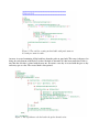
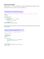
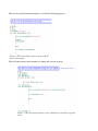
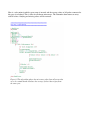
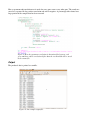
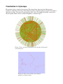
Visualisation of gene coexpression networks
Applied functional genomics 7.5 ECTS 2009
Supervisor Torgeir R. Hvidsten
By Peter Boman & Daniel Decker
Table of Contents
Introduction................................................................................................................................................2
Problem Description..............................................................................................................................3
User's manual and program access.............................................................................................................3
Program description...................................................................................................................................4
Input of probe to gene data....................................................................................................................4
Connecting probes to gene....................................................................................................................4
Choosing microarrays............................................................................................................................6
Output....................................................................................................................................................9
Visualisation in Cytoscape.......................................................................................................................10
Limitations................................................................................................................................................11
Conclusions..............................................................................................................................................11
Reference..................................................................................................................................................12
1
Introduction
Umeå Plant Science Center (UPSC) has during the years produced huge amounts of poplar microarray data(Sterky et al 2004). The microarrays have been produced from plants grown under different growth conditions and stresses. During this project we have compared data from different microarrays to investigate what genes that follows a similar expression pattern in the different microarrays. When these networks have been found this knowledge can be used to create experiments that verifies if these genes are coexpressed (Grönlund et al 2009).
Spearman rank correlation is used to asses whether to genes are coexpressed. Spearman rank correlation is a non­parametric method of measuring correlation, without any assumption of correlation between the variables. It is the pearson product calculated on ranks. Two sets are compared, by sorting after the values of one column, both columns are then ranked and the square of the difference between the ranks summarized, this value is the d2i in formula 1,
Formula 1: The pearson corelation coefficent.
This produced a number of coexpressed genes depending on the similarity of the analysed microarrays. The coexpressed genes was then visualised using a network drawing tool Cytoscape(TM) (Shannon et al 2003).
Problem Description
The program should be able to read an input file containing microarray data and a file that connects probes to genes. Each microarray consist of some ten thousand probes, some probes are unique while some are different probes from the same gene. Each probe got their own expression value. The probes that comes from the same gene needs to be averaged. One has to be able to select which arrays to compare to create coexpression values from trees grown in different conditions. The next step is to create an array profile with the averaged expression value of a gene from each of the selected microarrays. The created array is then compared, using Spearman's Rank Correlation, to all other genes to determine their correlation. The correlation values are then stored in an output file. The correlation values are finally used in a coexpression network, using cytoscape. The network consists of nodes that represent genes and edges that represent correlation above a certain threshold.
User's manual and program access
The program can be obtained by sending an email to [email protected] or [email protected] . The program requires that you are able to run perl programs and that you got input files in the right format. The required input files are as follows. The microarray datafile need to start with PU/exp followed by the name of the microarrays tab separated, subsequently followed by the name of the probe and the expression values tab separated and in the same order as the microarray they belong to. For example:
PU/exp
“array1” “array2”
PU00002 “value from array1” and so on. PU00001
“value from array1” “value from array2” The file that contains which probes that are connected to which genes need to start with PU “tab” before the probes in the format PUxxxxx can start. The first probe needs to be named PU00001 the second PU00002 and so on. Five tabs after the PUxxxxx the gene name should be presented. For example:
PU
PU00001
onetab twotab threetab
length” PU00002 onetab
twotab threetab
fourtab“gene name” “comments for variable fourtab“gene name” and so on. Our file can be downloaded from: http://www.populus.db.umu.se/data/genespring.tab
All data is case sensitive. Program description
The program is able to read different input files that supply the data for the probe to gene determination and correlation calculations, as long as the input is in the right format. Different microarrays can then be chosen by the user and correlation thresholds can be set. The code will here be described.
Input of probe to gene data
First a request for data is printed . The user may then insert a file name that will be opened. The program creates an array were each element is a line from the input file. Then each element is tab­
separated and pushed into a new data array.
Figure 1: The algorithm for reading in a text file and put each tab in and element in an array.
Connecting probes to gene
Since the data file starts with PU/exp the second element in the array has to be used as start value in the loop. A sub string is created from the two first characters from each element to see if they are “PU”. If this is true it is a probe and five elements later, five tabs later in the original data, in the array is the gene name. The probe name is then pushed into a hash as key with the gene name as value. If no gene name is present the gene is denoted with the probe name.
Figure 2: The code for creating an hash table with probe name as key and gene name as value.
An array is created containing all the hash keys from the probe to gene hash. This array is then used to bring out each element of the hash. It is then checked to determine if it has been run before. If this is true then the old value is joined with the new one. If not true a new key is created with the gene as key and array spot as value. The created hash is then printed. Figure 3: The algorithm to check whether the probe already exists.
Choosing microarrays
Which microarrays to examine is determined here and the accepted input format is specified. It is only critical that the arrays are separated by one character white space.
Figure 4: Input of microarray names.
Here an file name input is requested. The chosen microarray data file must be present in the same folder as your program.
Figure 5: Input of the file name were the microarray data is stored.
Here an array with all microarray names is created for indexing purposes. Figure 6: This algorithm creates an array with all microarray names.
Here all wanted arrays index numbers are found and stored in an array. Figure 7: The microarrays that are to be examined are stored in a separate array
Here is a sub routine in which a gene name is inserted and the average values of all probes connected to this gene is calculated. This is done for all chosen microarrays. The subroutine then returns an array with all values. Outlying and missing values will be removed.
Figure 8: This algorithm gathers the microarray value from all arrays that are to be examined and calculates the average of those that origins from the same gene.
Here a spearman rank correlation test is made for every gene versus every other gene. The results are sorted to a separate file for positive correlation and one for negative. A percentage ticker shows how large portion of the samples that has been screened
Figure 9: Here the spearman correlation is determined for between each gene and those with a correlation higher than the set threshold will be saved in the outout file.
Output
The produced data is printed to a textfile.
Figure 10: An example output file.
Visualisation in Cytoscape
The produced data is visualised in cytoscape. The picture below shows how the different genes correlate to each other. Green edges (lines) indicate positive correlation whereas negative correlation is shown by red edges. The gene are represented by nodes (dots). To simplify the picture a gene can be chosen together with its closest correlated neighbours as shown in fig 12.
Figure 11: An cytoscape visualisation of the positive and negative correlated genes.
Figure 12: A few genes with the genes that are positivly correlate to them.
Limitations
The file format needs to follow the examples exactly or the data and results will be corrupted. The program will not print any error messages if the input is wrong and will run through all steps. All input files needs to be placed at the same directory as the program. If PU in uppercase is present in other positions than in PU numbers your values might be distorted. All genes must have values in all examined microarrays, if values are missing the gene will be discarded. Conclusions
The program is able to calculate the spearman correlation between two vectors. As long as the data is in the right format. It is important to use several microarrays to minimize the amount of false positives due to random correlation. As approximately 15000 genes are compared this will give approximate 112 million comparisons, random positives are therefore likely to occur. In our test runs microarrays from poplar samples grown in long day, seven different microarrays, were evaluated. This resulted in around 10000 positively correlated hits with a correlation over 0.95 . Many of the genes are unknown and without extensive examination it is hard to determine whether this is a correct network of the coexpressed genes.
Reference
A. Grönlund, R.P. Bhalerao & J. Karlsson (2009) : Modular gene expression in poplar: a multilayer network approach. New Phytologist vol:181 p315­322
Shannon P, Markiel A, Ozier O, Baliga NS, Wang JT, Ramage D, Amin N, Schwikowski B, Ideker T (2003): Cytoscape: a software environment for integrated models of biomolecular interaction networks. Genome Research Vol 11 p: 2498­2504
Sterky F, Bhalerao RR, Unneberg P, Segerman B, Nilsson P, Brunner AM, Campaa L, Jonsson Lindvall J, Tandre K, Strauss SH, Sundberg B, Gustafsson P, Uhlen M, Bhalerao RP, Nilsson O, Sandberg G, Karlsson J, Lundeberg J, Jansson S (2004):
A Populus EST resource for plant functional genomics. Proc Natl Acad Sci. Vol 38 p: 13951­13956