1
GETTING STARTED WITH CARMEN 3 What can CARMEN do for Me? 3 What do I Need to Run CARMEN? 3 Running CARMEN the First Time 3 Working with Investigations Organizing your data Creating a new investigation Switching to Another Investigation Editing the Details of an Investigation Viewing Investigation Files Removing Investigations Discretizing Raw Data 4 4 4 6 6 7 7 28 LIMITING ANALYSIS BY SAMPLE ATTRIBUTES 8 PLOTTING DATA WITH CARMEN 9 Choosing Probes and Samples to Plot Choosing probes Grouping your samples Limiting the plot to a subset of your samples 9 9 9 9 Specifying the Plot Appearance Labeling your samples Sorting samples The location of the Key 10 10 10 10 Exporting Your Plot To Text 10 CALCULATING CORRELATIONS 10 Parameters Common to All Correlation Calculations File Name Minimum Correlation Statistical Test Sample limits Probe limits 11 11 11 12 12 12 Correlation: One Probe vs. All Others 12 Correlation: All Pairwise Correlations 12 Correlation: Differential Correlation 12 Calculating Correlation: the shortcut dialog 13 CALCULATING GENOME WIDE ERROR RATE SIGNIFICANCE FOR CORRELATION 13 CALCULATING DIFFERENTIAL EXPRESSION 19 Reducing the Effect of Outliers 19 Probe-wise Permutation Testing 19 WORKING WITH GENE ANNOTATIONS 21 Annotate a List of Genes 23 Finding Genes by Gene Ontology Annotation 23 Browsing the Gene Ontology file 25 Converting Genes to Probes 25 EXPORTING DATA 26 Viewing with Text Editors or Excel 26 Exporting integrated Datasets as Datasheets Chosing which samples to export Chosing which probes to export Datasheet File Format 27 27 27 28 Exporting Gene Frequency Lists from Rulesets 28 Exporting Rulesets to Cytoscape 30 Exporting Crosstabs of Rulesets 30 Exporting a Ruleset as Rules by Samples Datasheet 30 EXTERNAL APPLICATION AND ANNOTATION FILE LOCATIONS 30 Excel 30 Cytoscape 31 Species Gene Ontology Annotations 31 FILE FORMATS FOR CARMEN 32 File format overview 32 File format details Raw Data Probe Attributes 32 32 32 33 Sample Attributes Getting started with CARMEN CARMEN was written by David Quigley in Allan Balmain's lab at UCSF. Please do not re-‐distribute CARMEN at this time. Contact David by email: [email protected]. What can CARMEN do for Me? The principle functions of CARMEN are: • Plot gene expression data • Calculate Correlation between genes • Generate Correlation networks and export them to Cytoscape • Perform Association Rule Mining • Calculate Differential Expression between two conditions • Find annotations for genes, or genes which match a GO annotation What do I Need to Run CARMEN? CARMEN is currently compiled for OS X (Macintosh) and Windows machines. You will need the CARMEN package as well as data to analyze. Each data set consists of gene expression data, information about the probes that make up that gene expression file, and information about the samples in the experiment. CARMEN calls this set of three files an "investigation". You can load any number of investigations into CARMEN and switch between them at any time. Running CARMEN the First Time CARMEN tracks the locations of files that make up your investigations and various internal settings in a file called .carmen_properties. On Windows machines this file lives in whatever directory CARMEN was installed; on Macintosh machines it live sin your home directory. Note that this file starts with a period, so it may be hidden on your operating system. This file is not shipped with CARMEN, so the first time you run CARMEN the program will notice it does not exist and offer to create it for you: The first time you export a file to Excel or generate a network with Cytoscape, CARMEN will ask you for the location of the Excel or Cytoscape executable files (or .app files on OS X). Working with Investigations Each data set is organized into an Investigation. An investigation comprises a data file (a matrix of numbers with unique sample identifiers and unique probe identifiers), a "gene attributes" file which describes the probes, and a "sample attributes" file which describes the samples. The correct format for these files is described below. The investigation also specifices: • The folder on your hard drive where result files will be written • Whether your data are for mouse or for human (this affects the default annotation choice). Note that other organisms can be specified if you have annotation files for them. • What type of data are stored in this investigation (Gene Expression, Genotype, DNA Copy Number). This is useful if you will be building eQTL networks. • Which column in your gene attributes file should be used for the English-‐ language version of your probe (i.e. the Symbol) Organizing your data I suggest that you store your data in one location (e.g. "datasets") with a sub-‐folder for each investigation. I keep my investigations in a separate folder tree called "notebook". I find this helps me keep my intermediate files, which grow large and hard to track, away from my data directories, which should be kept clean. For example: /datasets /mouse_tails /mouse_skin_carcinomas /human_colon_carcinomas Creating a new investigation Choose File | New Investigation from the main menu. You'll see a dialog that looks like: Browse to the locations of the Raw Data, Sample Attributes, and Gene Attributes files. Brows to the Results folder. Pick a species. By default, the Data Type is Gene Expression. If your Gene Attributes file contains a column with the heading *Gene Name*, this will automatically be selected for the Gene Name Column. Otherwise, select the correct column. Your investigation should now exist. After creating your investigation, you should see its name in the main CARMEN window: Switching to Another Investigation Choose File | Open Investigation from the main menu. You'll this dialog: Pick the investigation you wish to open and click OK. Investigations you have opened recently will be sorted at the top of this list. Editing the Details of an Investigation Choose File | Edit Current Investigation from the main menu. You'll see a dialog that looks like: Here you can specify: • Raw Data, Sample Attributes, Probe Attributes The location of three main files that define the investigation. Click Browse to select a new file. • Result Directory The folder where results are written. Click Browse to select a new folder. • Species The species the investigation is associated with; this is used to pick a default value for GO annotations. Pick a new value from the drop-‐down. • Data Type What kind of data the investigation contains. In addition to gene expression data, CARMEN can be used for array Comparative Genomic Hybridization or genotype data. This is used if you plan to plot eQTL networks. • Gene Symbol Column The column in the probe attributes file that will be used as the "human-‐ readable" version of the probe identifier. This typically contains a gene symbol. Once you click OK, any changes you have made are written to the .properties file. Viewing Investigation Files You can view the Raw Data, Gene Attributes, or Sample Attributes files by selecting File | Show Gene Attributes, File | Show Sample Attributes, or File | Show Raw Data from the main menu. Removing Investigations To remove an Investigation from the CARMEN Investigation list, select File | Remove Investigation. This operation does not remove data or experiment files; it only takes the investigation out of the CARMEN .properties file. Limiting Samples by Sample Attributes Many operations in CARMEN can be limited to a certain subset of samples. All of these operations use the Sample Filter panel: Sample filter dialog, before any filters have been set You can limit samples by clicking Add Sample Limit. Limits are combined using a logical AND, so if several limits are specificed, only samples meeting ALL criteria will be kept. After a limit has been chosen, it can be removed by clicking on the limit and pressing the Remove button. The Sample Filter dialog looks like this: Sample filter dialog, Pressing OK will allow only samples where "treated" is "1" This simply reads out of the sample attributes file and allows you to specify either that you want samples that DO have a given property (in this case, samples where the "treated" column has the value "1") or that you want samples that DO NOT have a given property: Sample filter dialog, Pressing OK will allow only samples where "treated" is not "1" Plotting data with CARMEN To open the plotter, choose Export | Plot. You'll see a new dialog box. The left side is the control panel, and plots appear on the right side. Plot parameters, the left side of the plot dialog Choosing Probes and Samples to Plot Choosing probes CARMEN will attempt to plot all of the probes listed in the box labeled Probes. You can either paste or type probes into this box, one per line, or you can type the name of a gene into the Add Gene box and press the Add button. If there is only one probe with the gene name you've specified, it will be added to the Probes box. If there are multiple probes with that gene name, you will be prompted to select one probe to add. Grouping your samples You can group samples by any property found in the sample attributes file. All of the column headings from the sample attributes file will be populated into the Group By dropdown. For example, if you have a column header called sex, with values M and F, selecting sex will cause your samples to be grouped by M and F the next time you press Plot. Limiting the plot to a subset of your samples If you only want to show a subset of the samples, you can use the Limit To dropdown to select that subset. Note that you can either include all samples that meet some criterion (using the default "is" value) or you can exclude all samples that meet some criterion by switching "is" to "is not". Specifying the Plot Appearance Labeling your samples By default your samples are labeled with the IDENTIFIER column. You can choose any column in the sample attributes file for the label with the Labels dropdown; this is independent of the way the samples are grouped or sorted. Sorting samples If you check the Sorted checkbox, samples are sorted in ascending order using first probe listed in the probe box. If you are grouping your samples, they will be sorted within those groups. The location of the Key You can move the key to any corner of the plot using the Key dropdown. The plot can be made taller or wider using the Height and Width dropdowns. Exporting Your Plot To Text If you wish to take exactly the plot values you are currently looking at and export them to a text file, click Export. You will be prompted for the location where you want the file written. Calculating Correlations CARMEN can calculate several different kinds of correlation comparisons: • One probe vs. all other probes in the dataset • All probes vs. all other probes in the dataset • The different in correlation between pairs of probes in one condition vs. another condition (called "Differential correlation") The primary correlation dialog is reached from the main menu at Statistics | Correlation. There is also a simplified version of this dialog at Statistics | Correlation with one probe (described in the next section). The main Correlation dialog Parameters Common to All Correlation Calculations File Name Each correlation calculation creates a file in the experiments folder associated with this investigation. By default a unique file name based on the current date and time is provided; I recommend you provide a more informative file name. Each correlation file has the extension ".spear", so if you provide the file name "p53" then a file called "p53.spear" will be created. Minimum Correlation CARMEN will only report results where the correlation coefficient (either rho or p) is greater than this value, or less than -‐1 times this value. The default value of 0.7 was arbitrarily chosen and is not calculated to indicate a level of statistically significant correlation for your dataset. For differential correlation calculations (see below), at least one of the two conditions must have a coefficient significant at this level. Setting this value to zero would return all pair-‐wise correlations. Statistical Test By default, CARMEN uses the non-‐parametric Spearman Rank Correlation. When multiple values have the same observed value (and would therefore have the same rank, the tie-‐breaking algorithm differs slightly from that implemented by the R statistical programming environment. Ties are ranked using the mean of the ranks that are spanned, so (1,2,2,3) is ranked (1, 2.5, 2.5,4). CARMEN can also calculate Pearson correlation if that is selected in the drop-‐down. Sample limits You can restrict the correlation calculation to a subset of all samples with the Sample Limits control. If you do not add any sample limits, all samples will be used. If you are calculating Differential Correlation (see below), you must specify two non-‐ intersecting sets of samples. For details on the Sample Limits dialog, see the section Limiting Analysis by Sample Attributes. Probe limits You can limit calculation to those probes which do not have a value of NA (meaning there is a legitimate measurement for that value) at least some percentage of the time using the box labeled Minimum % Present. By default this value is 90%. Be aware that correlation results calculated using probes that are missing a substantial fraction of the time may be highly misleading. You can also limit calculation to those probes which have a minimum variance across all samples within the Sample Limits using the box labeled Minimum Variance. Variance is calculated for row X of length N as: SUM[ ( Xi -‐ mean(X) )2 ] / (N-‐1) Correlation: One Probe vs. All Others Specify the probe by typing in the name of the probe identifier or the Gene Symbol into the box labeled Seed. If you specify a gene that is matched by several identifiers, you will be prompted to choose one. Correlation: All Pairwise Correlations When you select the all pairwise correlations radio button, the seed box is replaced by a Limit to probes box. If you leave this box empty, all probes which meet the probe limits will be used. You can limit the all pairwise correlation calculation to a subset of all probes by pasting a list of probe identifiers (not gene names) into the box labeled Limit to probes. For your convenience, you can also add probes by ontology (see the section Finding Genes by Gene Ontology Annotation for details on how this dialog works). Correlation: Differential Correlation Differential correlation identifies pairs of probes where the difference in correlation coefficients between two sets of samples exceeds some user-‐provided value. This difference can occur whether both coefficients have the same sign or different signs, and can occur in either direction. To specify the minimal change in correlation between sample groups, set the box Minimum Change in Correlation to a value between 0 and 2. To specify that at least one sample group have a minimum magnitude of correlation, use the Minimum Correlation +/- box. To calculate Differential Correlation you must specify two non-‐intersecting sets of samples. For details on the Sample Limits dialog, see the section Limiting Analysis by Sample Attributes. Calculating Correlation: the Shortcut Dialog For the simple case when you wish to calculate one probe vs. all others, using all samples, you can use the simplified dialog Calculate Correlation, One Probe. This provides the same reuslt that would be obtained using the more complex Statistics | Correlation dialog Correlation for one probe vs. all, a shortcut to the main Correlation dialog Browsing Correlation Lists with the Correlation Viewer You can search within a correlation file using the Correlation Viewer, available at Statistics | Correlation Viewer. This is useful if you want to search within a large correlation file to ask quickly, "what is gene X correlated with under these conditions?" The Correlation Viewer is only available if you have selected a correlation file that was created in CARMEN. The Correlation Viewer To use the viewer, choose enter a gene name into the Gene Name text box and click Go. CARMEN will examine the currently selected correlation file and return all correlations between your chosen probe and other probes that exceed the correlation coefficient stringency specified in the Minimum Correlation: +/- text box. The Correlation Viewer, after searching for Aurka at a stringency of +/- 0.7 The results of the correlation viewer can be saved to a text file by clicking the Save button. Creating Correlation Networks After calculating correlation between a set of probes, CARMEN can represent correlated probes as a network by writing files which can be read by Cytoscape (www.cytoscape.com). Correlation is calculated in the same way whether the final output is a single file with a list of identifier pairs or a set of network files. However, several additional parameters can be set to modify the network that is created. In addition to correlation networks, where each node is a gene and each edge indicates correlation, CARMEN can generate eQTL networks. These are the same as correlation networks, with the addition of nodes representing loci in the genome and edges that represent influence between those loci and genes. These networks are described below. The Correlation Network dialog Correlation settings You specify the minimum correlation coefficient using the Minimum correlation +/- box. Any probe pair where the correlation coefficient is greater than or equal to this value or is less than or equal to -‐1 times this value will be plotted. For example, selecting 0.7 would include both the coefficients 0.75 and -‐0.8. The mathematical term for a the kind of network CARMEN generates is a graph. The term from graph theory for a network where each node is connected to all other nodes in the network is a "clique". The figure below demonstrates cliques of size 1, 2, 3, and 4: Cliques of size 1, 2, 3, and 4 You can choose to limit the nodes in networks generated by CARMEN to those nodes which are members of a clique of size 1, 2, 3, or 4 using the Minimum clique size dropdown. This can have the effect of returning a denser network which is enriched for functionally related genes. By default cliques are at least of size one, meaning there is no filtering. Note that identifying arbitrarily large cliques is computationally intractable in a large network. Choosing which probes are used to generate the network CARMEN refers to the probes used to generate the network as "seeds". In the simplest network, you pick a single seed, and CARMEN limits the network to that seed and all genes correlated with that seed at the level of correlation stringency you specify. To do this, either paste a single probe identifier into the large Seed Probes text box, or type a gene name into the text box below the large Seed Probes text box and press Add Gene. If there is only one probe identifier that matches that gene, it will be added to the seed box. If multiple probes match the gene, you will be prompted to pick one. You can enter any number of seeds into the seed box, including zero. If you specify no seeds, CARMEN will use all probes as seeds. This will generate a "genome-‐ wide" correlation network, which is often very large. If you specify more than one seed, the combination of all seeds and the genes correlated with each seed is used. For your convenience, you can also add seeds by ontology (see the section Finding Genes by Gene Ontology Annotation for details on how this dialog works). Creating a network from a list of probes You can limit the network to a set of seeds by clicking the Limit network to seeds checkbox. If you do this, CARMEN will not include genes correlated with your seed list in the network unless they are present in the seed list itself. Choosing which samples are used to generate the network You can restrict the correlation calculation to a subset of all samples with the Sample Limits control. If you do not add any sample limits, all samples will be used. For details on the Sample Limits dialog, see the section Limiting Analysis by Sample Attributes. Probe limits You can limit calculation to those probes which do not have a value of NA (meaning there is a legitimate measurement for that value) at least some percentage of the time using the box labeled Minimum % Present. By default this value is 90%. Be aware that correlation results calculated using probes that are missing a substantial fraction of the time may be highly misleading. eQTL Network Settings If you have used David Quigley's eqtl program (sorry, not yet published) to generate eQTL results, these results can be combined with correlation results to generate a combined correlation and eQTL network. If you select an eQTL result file by clicking the Browse button in the Expression QTL Settings section of the Correlation Network dialog, several new parameters appear: Inset of Correlation Networks Dialog: eQTL settings if you select an eQTL file You can limit the maximum permutation P value of connections in the eQTL network with the Maximum eQTL P value text box. By default, all eQTL in the source file will be included. If you check the Require that gene has an eQTL box, CARMEN will only plot genes that pass correlation stringency and also have an eQTL in the source file. If you check Allow genes with eQTL but no correlations, CARMEN will include genes in the network even if they do not have another correlated gene in the network. Network Node Attributes: Annotations and the Extra Attribute When CARMEN generate the network, it will attempt to add Gene Ontology attributes to each gene node from the relevant species ontology. You can choose the relevant species using the Annotation: dropdown. CARMEN will choose the species associated with this investigation, if you have specified this. You can also pick an additional column from the gene attributes file to associate with each node, provided that the value of this column is a number. This is useful if you wish to color the nodes in the network based on some other measured property. Note that attributes can always be added to networks after they have been created; see the Cytoscape documentation for details. Calculating Genome Wide Error Rate Significance for Correlation CARMEN can calculate the experiment-‐wise correlation significance as described in (Churchill & Doerge Genetics 1990) using the dialog at Statistics | Calculate GWER. Briefly, for each permutation, sample labels are permuted for each for pair-‐wise correlation calculation. The single strongest correlation obtained using scrambled labels is stored for each permutation. These values are then reported in the result file. To obtain the 5% GWER using N permutations, use the permutation correlation at position N * 0.05 in the ranked list (e.g. correlation 50 in a list of 1000). The probe identifiers reported in the file generated by this dialog are arbitrary; the only values of importance are the correlation coefficients. Correlation GWER dialog Calculating Differential Expression CARMEN can calculate a simple but useful measure of differential expression using the dialog reached from Statistics | Differential Expression. CARMEN calculates an unmodified t test for each probe when comparing values between two user-‐ specified sample groups. A t statistic is calculated for each probe, along with the mean value of that probe in each sample group. Reducing the Effect of Outliers By default, the 5th and 95th percentile of each gene is trimmed to reduce the effects of outliers. To turn off expression trimming, set the Expression trim % box to 0. Probe-‐wise Permutation Testing CARMEN can calculate probe-‐wise P values by performing permutations of the sample labels and comparing the strength of the permutation t statistic to the observed t statistic. Note that these values are not corrected for the number of tests performed. Do not report these P values as though they were corrected for mulitple testing! For a more robust treatment of differential expression, the user is refered to a tool such as Significance Analysis of Microarrays (Tusher PNAS 2001), available for the R statistical programming language or as a Microsoft Excel plug-‐in. Differential expression dialog. Association Rule Mining In addition to Correlation analysis, CARMEN can also perform Association Rule Mining as described in (Bayardo, Data Mining and Knowledge Discovery 2000). Briefly, this is a method for identifying features or combination of features that are frequently associated with a condition. The fundamental algorithm is called Apriori. For a description of the algorithm, please see the Bayardo et al. paper and related work in the data mining literature. The Association Rule Mining (or ARM) version implemented in CARMEN assumes that data have been discretized into three categories, which we will label "up", "down", and "no call". There are various ways to accomplish this; see the section Discretizing Raw Data for a description of the various options. The end result of discretization is the conversion of real-‐valued probe measurements into a set of features with values in the set {-‐1, 0, 1}, corresponding to {"down", "no call", "up"}. Rulesets generated by CARMEN have the extension ".ruleset". Core Rulesets have the extension ".core.ruleset". ARM Settings Support, confidence, and improvement When generating a new set of rules, you can specify levels of Support, Confidence, and Improvement that range between 0 and 100. For precise definitions of these terms see the ARM literature. Briefly, Support measures the percentage of samples where a given feature or combination of features (a feature set) is found. Confidence measures the degree to which a given feature set is present in one condition but not another. Improvement measures the change in confidence that occurs when a feature is added to a feature set. Therefore, higher values for support select for feature sets that occur more frequently. Higher values for confidence select for feature sets that discriminate between two classes. Higher numbers for improvement require more complicated rules to provide dramatically better fits to the data than simpler rules. Filtering rules by chi-‐squared statistic One way to evaluate a rule is by performing a chi-squared approximation for whether there is a significant difference in distribution of samples where the rule does and does not apply in one sample group vs. the other. You can limit rules returned by CARMEN to those where the P value for this chi-‐squared test is less than or equal to the value in Max Chi-sq P value. Filtering rules by rule complexity One measure of rule complexity is the number of features combined to generate the rule. CARMEN first generates all rules with one feature and then begins to create combinations of rules that have at least the minimal support level. CARMEN will combine up to as many rules are are specified in the Depth text box. For example, if Depth is three, then CARMEN can consider rules that combine three features. Note that if no one-‐ or two-‐ feature rules match the required degree of support, CARMEN will not consider three-‐feature rules. Discretization settings The implementation of ARM in CARMEN requires discretized data. For further information on how discretization works in CARMEN, see the section Exporting Raw Data After Discretization. Defining Class A and Class B Most analyses of ARM using CARMEN will define non-‐intersecting sample classes, arbitrarily termed Class A and Class B. These classes can be defined using Sample Limits, as described in the section Limiting Samples by Sample Attributes. Additionally, you may define classes by using properties of one or more genes after they have been discretized. For example, if you wish your groups to consist of "samples where Aurka is called 'up' " and "samples where Aurka is called 'down' ", you can specify these with the gene attributes Sample Filter dialog: The Gene Attributes Sample Filter dialog, before a gene has been entered To use this panel, enter the symbol for a gene next to the box labeled Find identifiers for gene and click Search. If only one probe identifier matches, it will be selected automatically. If more than one matches, click on the desired probe identifier. Choose either is or is not from the logical dropdown, and then Up or Down from the direction dropdown. Note that you can select "No Call" cases by selecting "is not"; for example, you could choose "Per3 is down" for one sample set and "Per3 is not down" for the other. Creating Core Rulesets To increase the robustness of rulesets, CARMEN can create Core Rulesets. These are generated by performing a "leave one out" analysis that generates all sample sets where a single sample has been removed from the analysis and uses the same ARM parameters to creates rules. Any rule that appears in all of the "leave one out" rulesets is considered a "Core Rule". This is similar in spirit to a cross-‐validation exercise. Core Rulesets will have the same filename as the original ruleset, but with the extension ".core" added to the file suffix. Working with Gene Annotations Annotate a List of Genes Given a list of gene names, CARMEN can report back simple annotation information: • Physical location in the genome • Gene Ontology identities associated with the gene To open the Annotate gene list dialog, select Annotation | Annotate genes from the main menu. Gene names can be pasted into the box visible when the dialog is opened. Annotate gene list dialog If you wish to identify each gene in a file previously generated by CARMEN (e.g., a correlation result file) then navigate to that file and open the Annotate gene list dialog. The "Genes in currently selected file" radio button will be enabled, allowing you to choose to have CARMEN read from that file: The results of the annotation are written to a file that is called, by default, annotation.txt. You are prompted to choose a file location after clicking the OK button. Gene locations drawn from the UCSC genome browser's most recent build at the time CARMEN was released. Gene Ontology annotations are drawn from the most recent Homo sapiens and Mus musculus annotations available from geneontology.org at the time CARMEN was released. Finding Genes by Gene Ontology Annotation You can identify genes annotated to belong to various Gene Ontology categories by opening the Annotation | Find genes by GO dialog. To search, enter a GO term into the case-‐insensitive GO Term text box. Queries will return all terms whose name contains an exact match for that query (e.g. "wnt" returns "Wnt-‐protein binding" among many others). Search by GO terms, after entering wnt into GO Term and pressing Search Selecting one or more matching terms will search for those genes in the currently loaded investigation, using the Gene Symbol column the user has indicated. Any matches will be loaded into the Genes and Probes text boxes. Note that on some array platforms, more than one probe can match a single gene name. Note that the completeness of GO annotation searches in CARMEN is limited by the completeness of the underlying annotations. These annotations, while invaluable, are not complete by any means and should only be a starting point for any analysis. Search by GO terms, after searching for wnt and selecting Wnt-protein binding To extract these gene names or probes, simply copy them out of the text boxes. Browsing the Gene Ontology File If for some reason you wish to examine the Gene Ontology file used by CARMEN, you can see it by selecting Annotation | Show GO File. Note: there are two basic data structures used by CARMEN to return Gene Ontology results: 1. The Gene Ontology file. This defines the list of valid GO terms, along with their GO identifiers and which major branch of the GO tree they belong to 2. Individual species ontologies. This defines the list of genes that have been associated with a particular GO identifier in a given species. Note that CARMEN does not store the relationships between GO terms and does not perform Gene Ontology enrichment analysis. For that, I recommend a dedicated tool such as BiNGO (Maere Bioinformatics 2005). Converting Genes to Probes If you have a list of genes and wish to know which probe identifiers correspond to that gene list, you can use the dialog at Annotation| Convert Genes to Probes to perform this conversion. Paste in a list of gene names into the box labeled Genes, one gene per line, and press the Convert button. Genes to probes dialog Genes to probes dialog, after converting Kras and Hras1 to probe identifiers Exporting Data Viewing with Text Editors or Excel All of the analysis files generated by CARMEN are text files, so the Export | To Text Editor command is simply a shortcut to open the data you're looking at in your default text editor. In Windows this is, by default, Notepad. Notepad is inadequate for anything but the most trivial use, and I recommend TextPad for Windows users. For the Macintosh, the default text editor is TextEdit. This is slightly better than Notepad, but a more robust text editor such as TextMate or Emacs is a better choice. The Export | To Text Editor menu item is disabled unless you have selected an analysis result that can be viewed in a text editor. Any analysis file that can be viewed in a text editor can also be viewed with Microsoft Excel, if you have Excel installed on your machine. Use Export | To Excel to open analysis files in Excel. WARNING: Excel automatically mangles the names of many genes by turning them into dates (e.g. MARCH8, SEPT9 etc.). Once this is done, you cannot convert the names back. I do not recommend Excel if you are working with gene names. Exporting Integrated Datasets as Datasheets It is sometimes useful to export a dataset file that contains expression, sample, and gene attribute data all in one file. CARMEN can create such an export with the dialog at Export | To Dataset. Export To Dataset, default view Chosing which samples to export Samples to be exported can be chosen with a Sample Limits dialog. For more details on this dialog, see the section Limiting Analysis by Sample Attributes. Chosing which probes to export You have three choices: 1. Use all probes. This is the default. 2. Probes in the selected file. This is only available if a file generated by CARMEN is currently selected before the Export To Dataset dialog is launched. 3. Probes pasted into a text box. To limit the dataset to a subset of probes, select Paste probes into box and probes into the box that appears, one gene per line. You can use the Add by Ontology button to add probes that match a particular Gene Ontology annotation; see the section Finding Genes by Gene Ontology Annotation for details. In all cases, you can restrict the probes written by the percent of the time they are called "present" in the samples you have selected to export. By default, the minimum percent present is zero, so all probes are exported. Export To Dataset, limit dataset by probes selected Datasheet File Format As the original use for this dialog was compatibility with the TMEV TM4 Microarray software suite (www.tm4.org), the file that is generated is exactly the correct format to be imported natively by that program. The format is: PROBE_ID<tab>Name<tab>Sample1<tab>Sample2<tab>SampleN <tab>IDENTIFIER<tab>Sample1<tab>Sample2<tab>SampleN <tab>sample_attribute_1<tab>value1<tab>value2<tab>valueN <tab>sample_attribute_2<tab>value1<tab>value2<tab>valueN <tab>sample_attribute_N<tab>value1<tab>value2<tab>valueN gene_identifier_1<tab>gene_name_1<tab>value1<tab>value2<tab>valueN gene_identifier_2<tab>gene_name_1<tab>value1<tab>value2<tab>valueN gene_identifier_3<tab>gene_name_1<tab>value1<tab>value2<tab>valueN Exporting Raw Data After Discretization Gene Expression data is typically expressed as a real-‐valued number (i.e. a number with any value). Some kinds of investigations operate on categories (e.g. "LOW", "HIGH", or "NO CALL"), which can be obtained by discretizing the raw data. This means to convert the real-‐valued numbers in a Raw Data file to be have the values {-‐1, 0, 1} depending on some threshold. You can generate a discretized version of your raw data by selecting Export | Raw Data Discretized. This will bring up a dialog that looks like: Export Raw data as Discretized Data dialog From here you can choose a method of discretization, a bound, a file name to write, and you can limit the samples to be used (see Limiting Samples by Sample Attributes for an explanation of how this simple dialog works). The following methods of discretization are currently implemented: • No Discretization Passes through the raw data • Standard Deviation Calculate the mean and standard deviation of each row of probes. Samples that are more than [mean + (bound * standard deviation) ] are marked as one; samples less than [mean -‐ (bound * standard deviation) ] are marked as negative one. All other samples are marked as zero. • Median Deviation Same as Standard Deviation, but uses the Median and Median Absolute Deviation. • Absolute Cutoffs Values greater than bound are marked as one; values less than negative bound are marked as zero; values in between are marked as zero. Useful for aCGH data. • Percentile For each probe, calculates the percentile into which each value falls; values greater than the higher percentile are marked one, less than the lower percentile are marked negative one, in between are marked zero. • Standard Deviation by Sample Calculates the mean and standard deviation across all probes in a sample (as opposed to all samples in a given probe) and marks them as in Standard Deviation. Exporting Gene Frequency Lists from Rulesets CARMEN can count the number of times each gene appears in an analysis file that it created and export that count as a simple list. To do this, select Export | Gene Frequency List. This feature is only enabled if you have selected a file generated by CARMEN. Exporting Rulesets to Cytoscape CARMEN can generate a view of Association Rule Mining rulesets using Cytoscape if you select a ruleset and choose Export | To Cytoscape. Note that each rule will be drawn as a separate node in this view, so the rule "AURKA_is_-‐1" (Aurora Kinase A is low) would be drawn separately from "AURKA_is_1" (Aurora Kinase A is high). Exporting Crosstabs of Rulesets CARMEN can generate a crosstab view of Association Rule Mining Rulesets if you select a ruleset and choose Export | Crosstab of rules. This generates a file where the individual constituents of each rule are listed as rows and columns, with an integer indicating the number of times these two elements appear together in a rule. The upper right and lower left triangles of this matrix are identical. Exporting a Ruleset as Rules by Samples Datasheet CARMEN can generate a datasheet view of a ruleset where each row is a rule, each column is a sample, and the elements have the value one if the rule applies to that sample and a zero otherwise. The format of this datasheet is described above in the section Exporting Integrated Datasets as Datasheets. External Application and Annotation file locations Excel You can open files CARMEN generates directly in Microsoft Excel if you have it installed. The first time you export a file to Excel (Export | To Excel), CARMEN will ask you to browse to the location of the Excel application file. If for some reason you move Excel, you can update this location by selecting File | Edit Carmen Properties and browsing to the new file. The Carmen Properties dialog Cytoscape CARMEN can calculate correlation networks and export these networks to be visualized in Cytoscape (www.cytoscape.org). The first time you export a file to Cytoscape, CARMEN will ask you to browse to the location of the Cytoscape application file. If for some reason you move Cytoscape (or upgrade to a new version with a different location or file name) you can indicate the new Cytoscape application from File | Edit Carmen Properties. Cytoscape uses a file called a "vizmap" file to tell it what graphs should look like; if you are an experienced Cytoscape user and wish to change the default vizmap file used when CARMEN exports cytoscape files, you can change this from the same dialog. Species Gene Ontology Annotations CARMEN ships with a current copy of the Gene Ontology (www.geneontology.org). This file is stored in a compressed format. If an updated version of this file is released by David, you can browse to that file in this dialog. CARMEN also ships with versions of the species-‐specific Gene Ontology files for Mus musculus and Homo sapiens. If you wish to add a new annotation, you can do that from this dialog as well. Adding a new annotation will cause that species to appear in the Investigation drop-‐downs that allow you to specify which species to associate with the investigation. File formats for CARMEN File Format Overview I describe experimental result sets with three files: one describing samples, one with raw data, and one describing the probes/genotypes/whatever. I refer to these as the "probe attributes", "sample attributes", and "raw data" files. All files should be tab-‐delimited text. Format instructions will refer to "rows" (lines) and columns (separated by tabs) starting at (1,1) in the upper left corner. Element (1,1) should always be the word "IDENTIFIER" (no quotes) in upper-‐case. To run an eQTL analysis, you will need two sets of these files: one for genotypes and one for expression data. The sample identifiers for genotypes and expression data might not be identical for this analysis, so one column in the sample attributes for genotypes must contain the identifier of the corresponding sample in the raw data sample attributes. If there is no corresponding sample (e.g. you have a genotype but no matched expression) the value of this column should be "NA" for that row. File Format Details Raw Data • The first row consists of the IDENTIFIER element followed by a list of unique sample names. These samples will be described in the sample attributes file. • The first column consists of the IDENTIFIER element followed by a list of probe identifiers. These probes will be described in the probe attributes file. • The remainder of the file consists of the measurement for a given probe at that sample. IMPORTANT: Missing values in this file are coded as any non-numeric value. I recommend using "NA" rather than a dot. Sample identifiers should start with a letter, not a number, as this makes downstream analysis using R easier. Example: IDENTIFIER sample01 sample02 1444519_at 12.5 NA 1418175_at 9.4 6.6 In this example, there are two samples named sample01 and sample02 and two probes with the identifiers 1444519_at and 1418175_at. The 1444519_at measurement for sample02 is missing. Probe Attributes The first column consists of the IDENTIFIER element followed by a list of probe identifiers. The first row consists of the IDENTIFIER element followed by zero or more properties we wish to store about these probes. Example properties might include "Chromosome", "refseq_id", "location_Mb", "cM", or anything we know about the marker. There is one special column called "Gene Name"; this will be the human-‐ readable name for the probe that is displayed by various programs. It is required for eQTL analysis. Missing values should be coded as "NA". Missing values should not be empty. Example: IDENTIFIER symbol Chr 1444519_at Lgr5 10 1418175_at Vdr 15 For files describing genotypes (SNPs, RFLP, etc) it is very convenient if the Gene Name column indicates the physical location of the probe and can be sorted by simple alphanumeric order. For example, "Chr05.012.024" for a SNP on chromosome 5 at 12 Mb, 24 Kb can easily be sorted in physical order. Contrast with "5.800", which will sort before "5.112000000" Sample Attributes This file has the same format as Probe Attributes, but each row describes a sample instead of a probe. Example: IDENTIFIER symbol age sample01 M 32 sample02 F NA