Download Development of a PC-Based Object-Oriented Real

Development of a PC-Based
Object-Oriented Real-Time
Robotics Controller
by
Hang Tran
A thesis
presented to the University of Waterloo
in fulfillment of the
thesis requirement for the degree of
Master’s of Applied Science
in
Mechanical Engineering
Waterloo, Ontario, Canada, 2005
©Hang Tran, 2005
I hereby declare that I am the sole author of this thesis.
I authorize the University of Waterloo to lend this thesis to other institutions or individuals for the
purpose of scholarly research
Signature
I further authorize the University of Waterloo to reproduce this thesis by photocopying or by other
means, in total or in part, at the request of other institutions or individuals for the purpose of scholarly
research.
Signature
ii
Abstract
The industrial world of robotics requires leading-edge controllers to match the speed of new
manipulators. In order to improve the performance of the Deltabot, an ultra high-speed cable-based
robot, a new controller called the QNX Multi-Axis Robotic Controller (QMARC) was developed.
QMARC is a PC-based controller built for the replacement of the existing commercial controller
called PMAC, created by Delta Tau Data Systems. Although the PMAC has its own real-time
processor, the rigid and complex internal structure of the PMAC makes it difficult to apply advanced
control algorithms and interpolation methods. Adding unconventional hardware to PMAC, such as a
camera and vision system is also quite challenging. With the development of QMARC, the flexibility
issue of the controller is resolved. QMARC’s open-sourced object-oriented software structure allows
to the addition of new control and interpolation techniques as required. In addition, the software
structure of the main Controller process is decoupled for the hardware, so that any hardware change
does not affect the main controller, just the hardware drivers. QMARC is also equipped with a userfriendly graphical user interface, and many safety protocols to make it a safe and easy-to-use system.
Experimental real-time test has proven QMARC to be a reliable real-time system. Despite minor
fluctuations in the servo loop periods, the controller can still achieve close path tracking running at
2.5 kHz.
In comparing the PMAC and QMARC controller performance on two pick-and-place
paths, it was found that for both paths QMARC yielded better results than PMAC on all three motors
of the Deltabot. Accumulated following error for the PMAC was at least one order of magnitude
greater than QMARC, and QMARC was more easily tuned than PMAC. These experimental results
show that QMARC is a reliable and safe controller with consistent results.
The stable software foundation created by the QMARC will allow for future development of the
controller as research on the Deltabot progresses. Its open source structure will ease the way for new
researchers implementing software modules such as servo control algorithms and trajectory, or new
hardware like grippers and vision sensors, creating a flexible and powerful system that can be used
for many applications.
iii
Acknowledgements
For the past two years, I have received a generous amount of help and guidance from my supervisors,
Dr. Amir Khajepour and Dr. Kaan Erkorkmaz. I would like to thank Dr. Khajepour for taking me
into the Robotics research group, which has provided me with both practical experience in robotics
control, and academic experience in the development of new robotic manipulators, such as the
Deltabot. I also thank Dr. Erkorkmaz for sharing his knowledge and expertise in control systems,
trajectory generation and software development, which was pivotal in my research.
I take great pride in my work, but where would I be without the help of my peers and colleagues. I
would like to give a big hug to Edmon Chan for his insight into all things mechanical and electrical,
Saeed Behzadipour for his assistance in my research, Gireesh Dharwarkar for keeping me on my toes,
and Matthew Asselin for sharing his knowledge of the QNX operating system with me without
hesitation.
With all of the software and hardware implementation involved in this project, I would like to
graciously thank Robert Wagner, Andy Barber and Steve Hitchman, our fine technicians, for their
help and kindness to us pesky students.
I would like to thank my family for their undying support when I told them that I wanted to
continue my education and especially my boyfriend, Neil Lonsdale, for encouraging me and picking
me up when things went astray in my research.
Last, but not least, I would like to acknowledge the financial support of Materials and
Manufacturing Ontario (MMO) in this research. Without their support our ideas could not have been
realized.
iv
Contents
Chapter 1
Background................................................................................................................. 1
1.1
Deltabot .................................................................................................................................. 1
1.2
PMAC..................................................................................................................................... 3
1.3
QNX Real-Time Operating System........................................................................................ 4
1.4
Object-Oriented Software Design .......................................................................................... 6
1.4.1
Reusability...................................................................................................................... 6
1.4.2
Encapsulation ................................................................................................................. 7
1.4.3
Inheritance ...................................................................................................................... 7
1.4.4
Polymorphism................................................................................................................. 8
1.4.5
Operator Overloading..................................................................................................... 9
1.4.6
Constructors and Destructors.......................................................................................... 9
Chapter 2
Literature Review..................................................................................................... 10
2.1
PC-Based Controllers ........................................................................................................... 10
2.1.1
Distributed Multiprocessor Control Systems ............................................................... 11
2.1.2
Single-Processor Host and DSP Control Systems ........................................................ 12
2.2
Object-Oriented Software Design in Robotic Controllers.................................................... 13
2.3
Robot Control Structure ....................................................................................................... 16
2.3.1
Trajectory Generation................................................................................................... 16
2.3.2
PID Control Algorithm................................................................................................. 18
Chapter 3
Design and Implementation..................................................................................... 21
3.1
Overview .............................................................................................................................. 21
3.2
Hardware Setup .................................................................................................................... 22
3.3
Process Structure of the QMARC ........................................................................................ 23
3.3.1
QNX Message-Handling Functions.............................................................................. 25
3.4
Design of the Controller Console ......................................................................................... 27
3.5
Design of the Starter Process................................................................................................ 29
v
3.6
Design of the Hardware Server ............................................................................................ 32
3.7
Design of the Timer.............................................................................................................. 34
3.8
Design of the Controller ....................................................................................................... 35
3.9
Running the Controller ......................................................................................................... 44
3.10
Safety Features ..................................................................................................................... 44
3.10.1
Hardware Limit Switches ............................................................................................. 44
3.10.2
Software Position Limits .............................................................................................. 45
3.10.3
Following Error Limit .................................................................................................. 46
3.11
Control Algorithm ................................................................................................................ 46
3.11.1
3.12
Notch Filter................................................................................................................... 48
Trajectory Generation........................................................................................................... 48
3.12.1
Offline Cubic Spline Trajectory Generation ................................................................ 49
3.12.2
Online Position-Velocity-Time (PVT) Trajectory Generation..................................... 50
Chapter 4
Software Design Issues............................................................................................. 52
4.1
Timing .................................................................................................................................. 52
4.1.1
POSIX Timer vs. QMARC Timer................................................................................ 53
4.2
Data Logging ........................................................................................................................ 54
4.3
Memory Allocation of Variables.......................................................................................... 55
Chapter 5
Software Testing and Analysis ................................................................................ 57
5.1
Real-Time Behavioural Tests and Results............................................................................ 58
5.2
Controller Performance Tests and Results ........................................................................... 60
5.2.1
Standard X-Z Plane Path Test ...................................................................................... 61
5.2.2
Rotated Standard Path Test .......................................................................................... 69
5.3
Reproducibility Tests and Results ........................................................................................ 75
Chapter 6
Conclusions ................................................................... Error! Bookmark not defined.
Chapter 7
Recommendations ........................................................ Error! Bookmark not defined.
Bibliography
.................................................................................................................................... 83
vi
vii
List of Figures
Figure 1-1: General structure of the Deltabot [5] ................................................................................ 2
Figure 1-2: Encoder Conversion Table Process [6] ............................................................................. 3
Figure 1-3: Class inheritance code example ........................................................................................ 7
Figure 1-4: Polymorphism class declaration example ......................................................................... 8
Figure 1-5: Polymorphism function call example ............................................................................... 9
Figure 2-1: Block Diagram of Kriegman and Siegel hand control system [18] ................................ 12
Figure 2-2: QMotor 2.0 Hardware/Software Architecture [33]......................................................... 15
Figure 2-3: Class Hierarchy of QMotor Robotic Toolkit Platform [33]............................................ 16
Figure 3-1: QMARC Control Structure ............................................................................................. 22
Figure 3-2: QMARC Process Communication Structure .................................................................. 24
Figure 3-3: Message Structure for Client-Server Communication .................................................... 25
Figure 3-4: Example code for client-server communication and message-handling ......................... 26
Figure 3-5: QMARC Photon Graphical User Interface (GUI) .......................................................... 29
Figure 3-6: Flow Chart of Starter Process ......................................................................................... 31
Figure 3-7: Flow-chart for Hardware Server ..................................................................................... 33
Figure 3-8: Code for Timer ISR and Setup Procedure....................................................................... 34
Figure 3-9: Class structure of robotic motion controller.................................................................... 36
Figure 3-10: Flow-chart of algorithm for offline trajectory generation control loop, ctrlLoop() ...... 41
Figure 3-11: Flow-chart of algorithm for online trajectory generation control loop,
ctrlLoopOnlineTraj() ................................................................................................................. 42
Figure 3-12: Schematic of PID Feed-Forward Velocity and Acceleration Control Algorithm ......... 47
Figure 3-13: Schematic of path for PVT online trajectory generation............................................... 50
Figure 4-1: Memory allocation code sample ..................................................................................... 55
Figure 5-1: Real-Time Servo Loop Period Variation in a Step Input Test ........................................ 59
Figure 5-2: Standard X-Z Plane Path in Cartesian Space .................................................................. 61
Figure 5-3: X-Z Plane Path – Arm Positions with Selected Path Knots............................................ 61
Figure 5-4: X-Z Plane Path – End-Effector Position using PMAC and QMARC............................. 62
Figure 5-5: X-Z Plane Path - Arm Positions for PMAC and QMARC with Cubic Spline................ 63
viii
Figure 5-6: X-Z Plane Path - Arm Position Errors for PMAC and QMARC with Cubic Spline ...... 65
Figure 5-7: X-Z Plane Path - Command Velocity using PMAC and QMARC with Cubic Spline .. 66
Figure 5-8: X-Z Plane Path – Command Velocities for PVT and Cubic Spline on QMARC ........... 67
Figure 5-9: X-Z Plane Path – Arm Position Errors with PVT and Cubic Spline on QMARC .......... 68
Figure 5-10: X-Z Plane Path - Command Acceleration..................................................................... 69
Figure 5-11: Rotated Standard Path in Cartesian Space .................................................................... 69
Figure 5-12: Rotated Path - Arm Positions with selected path knots ................................................ 70
Figure 5-13: Rotated Path - End-Effector Position for PMAC and QMARC.................................... 70
Figure 5-14: Rotated Path – Arm Position for PMAC and QMARC ................................................ 72
Figure 5-15: Rotated Path – Arm Position Error for PMAC and QMARC ....................................... 73
ix
List of Tables
Table 1: QMARC Controller Gains................................................................................................... 60
Table 2: Arm Position Errors (in radians) for PMAC and QMARC using Cubic Spline .................. 64
x
Chapter 1
Background
Robotics is being used for increasingly more applications in different industries.
The mass
production of everything from cars to surgical needles requires precision repetitive work ranging from
assembling parts, welding, machining, and pick and place tasks. To control these robots, engineers
have built a multitude of controllers using Programmable Logic Controllers (PLC’s), Digital Signal
Processing (DSP) boards and Personal Computers (PC’s). Although PLC’s are still widely used in
industry, research in the past decade or so has been concentrated on the development of PC-based
controllers for industrial applications. Typically, DSP controllers with host computers have been
used as controllers, however the high cost and complexity have made PC-based controllers a desirable
field of research. In this work, a single-processor PC-based controller was developed for a three
degree-of-freedom ultra high-speed cable-based parallel robot, named the Deltabot, created at the
University of Waterloo [1], [2].
1.1 Deltabot
The Deltabot was designed based on the Stewart Platform [3], a six degree-of-freedom mechanism
developed for flight simulations that used six linear actuators in parallel created in 1965. The parallel
structure of the Deltabot is depicted in Figure 1-1. This cable-based robot is among a new line of
high-speed robots built for pick-and-place operations. In its novel design, there are three motors
attached to three aluminum arms that control the location of the end-effector through a set of
lightweight cables. The end-effector is attached to a central shaft that is pressurized to keep the
cables in tension. By using cables instead of rigid links, the inertia of the manipulator is minimized,
thus allowing high accelerations of 2g. Currently, this prototype can run a 35cm path at 120 cycles
per minute [4].
1
Figure 1-1: General structure of the Deltabot [5]
Parallel manipulators have distinct advantages over serial chain-link counterparts, namely, greater
stiffness, higher precision and less inertia. However, these advantages come at the cost of singular
configurations in the workspace, and smaller and more complex workspaces.
For parallel
manipulators, computation of the forward position kinematics is a challenging task involving nonlinear equations. Whereas the inverse position kinematics calculation is relatively straightforward.
This is opposite to kinematic calculations for serial manipulators. Due to the nature of parallel
manipulators, more computation is required for proper control of the robot [4]. In addition, more
advanced control algorithms must be considered for the Deltabot because, not only is it a parallel
manipulator, but it also has cable-based links. In spite of disadvantages with control and workspace
issues, parallel manipulators offer promising performance speed and precision for pick and place
operations.
2
1.2 PMAC
Currently, the Deltabot uses a general-purpose commercial controller called the Programmable
Multi-Axis Controller (PMAC) version 2.0 made by Delta Tau Data Systems Inc [6]. The PMAC
does not perform the inverse or forward position kinematics on the manipulators, but rather it
performs control based on joint coordinates. This controller is composed of a real-time multi-tasking
computer with DSP technology. Although the PMAC has the capability to control up to eight motors
simultaneous on eight separate coordinate systems, each standard PMAC 2.0 module controls only
four motors. The software architecture of the PMAC is complex and somewhat hidden to make it
simpler for users. What is known is that each PMAC module contains four encoder inputs, which
each has hardware encoder counters with associated timers. As shown in Figure 1-2, at the end of
each servo cycle, a servo interrupt is sent to latch the counter values and store them in a software
structure called the Encoder Conversion Table. This Encoder Conversion Table consists of two
columns: X memory and Y memory. In X memory, the actual 24-bit value of the encoder position is
stored in the highest word. The rest of the X memory contains intermediate values. Memory Y
contains the information required to process and convert the position value so that it can be stored in
the X memory location. Y memory consists of a 16-bit address of the source of the encoder that it is
reading from plus an 8-bit value of the conversion method performed on the encoder value. The
actual position is then extended to 48-bits by the software, which also multiplies the value by a
position-scaling factor. Actual encoder positions are used as feedback data for the servo control loop.
When the new servo control signal is calculated, the signal is sent at an opto-isolated set of Digital to
Analog Converters (DAC) that are connected to the motor amplifier.
Figure 1-2: Encoder Conversion Table Process [6]
3
Although the PMAC has a wide range of options and an impressive range of capabilities that allow
users to tailor the controller to each application, the process of understanding the PMAC architecture
and modifying its programming is very slow and sometimes difficult due to the complexity of the
PMAC system. Adding unconventional components to the controller, such as a vision system, can be
quite challenging, time-consuming and costly.
Due to the complex nature to the Deltabot’s
mechanical structure, more advanced control algorithms must also be considered for control of this
cable-based manipulator.
In order to minimize hardware costs as well as allow for higher system flexibility in the controller,
the PC-based controller was developed for motion-control of the Deltabot. The open-source code of
the PC-based controller will allow future research to quickly produce controllers with advanced
control algorithms for the Deltabot, along with the incorporation of sophisticated trajectory generation
techniques, which cannot be performed by the PMAC.
In this research, a single-processor PC-based motion controller was developed on a real-time
operating system called QNX Neutrino 6.0. This controller is named the QNX Multi-Axis Robotic
Controller or QMARC. A literature review on different aspects of the real-time control systems will
be discussed in Chapter 2. The detailed software design of the controller, from its object-oriented
software structure to its control algorithm and safety features will be covered in Chapter 3. Chapter 4
will review the issues that arose during the development stage such as timing, logging data, and
memory management, followed by the experimental results of the PC-based controller compared to
the PMAC performance in Chapter 5. To produce comparable results, the PC-based controller was
programmed with similar control and trajectory generation algorithms as the PMAC.
The
conclusions of this research along with details on future work will be discussed in Chapter 6.
1.3 QNX Real-Time Operating System
An operating system (OS) is a software platform on computers that manages resources, and controls
memory and peripheral devices. Its responsibilities include performing all input/output operations
and efficient use of devices [7]. In order to qualify as a real-time operating system (RTOS), the OS
must be able to perform duties within a given time constraint, whether that objective time is measured
in microseconds or milliseconds. A RTOS must also be able to handle simultaneous tasks that are
triggered asynchronously as well as have an effective method of scheduling these tasks. The main
function of the RTOS is to allocate processor time to different processes and have the ability to stop
4
and resume any task. QNX Neutrino 6.0 is an example of a RTOS developed by QNX Software
Systems. The QNX operating system is a modular operating system with high fault tolerance, in the
case of a device driver failing, the entire OS will not crash. A thorough analysis of different
commercially available real-time operating systems was not the objective of this research. Instead,
QNX was found to be the most economically choice for a RTOS that was suitable for development of
the motion controller.
In a motion controller, there are multiple tasks that need to be performed simultaneously, such as
monitoring limit switches, performing input/output operations to hardware, and performing the
control loop and online trajectory generation on multiple motors. Saying that an RTOS can run
multiple processes simultaneously, however, does not necessarily mean that the speed of task will be
completed more quickly. This is because the computer usually still has only one processor and
multiple tasks are not truly run “concurrently”. There are different methods of scheduling processes
so that each task can have a chance to run on the processor according to their priority, a numerical
value assigned to each process. In priority-based execution, a ready process with higher priority will
run first and to completion if the processor is idle. In pre-emptive priority-base execution, any task
can be stopped, or pre-empted, if a higher priority task is suddenly ready, and the interrupted task will
only continue when the high priority task is completed [8]. QNX uses pre-emptive priority-based
scheduling with two different types of scheduling algorithms: First-In First-Out (FIFO) and Round
Robin (RR) with 64 priority levels.
In FIFO scheduling a task can run on the processor as long as it wants, unless a higher priority task
is ready to run. Tasks with the same priority are locked from running, and wait in a first-in first-out
queue. Lower priority tasks get an opportunity to run when there are no other tasks ready. RR
scheduling is pretty much the same as FIFO except tasks can only run for a predefined timeslice that
can be set by the programmer. If the task is not complete after the timeslice is up, another task with
the same priority will have the opportunity to run. For this research, RR scheduling is used for all
processes and threads. A process refers to any application running on the processor, whereas threads
are created from within a process and typically run smaller segments of code for increased parallelism
in the software.
In QNX multiple processes can communicate through “message-handling”. The idea of message
handling is that one process can send a message to another process to trigger an action in the other
process or simply to deliver or request data. When the second process has handled the message, it
sends a reply message back to the first process, which also unblocks it. To prevent dead-locking, a
5
phenomenon with multiple processes whereby all process are blocked waiting for a message, it is
common practice to only send messages that request action or information to a server. A server is a
process that runs in an infinite loop waiting for messages from client processes. In client-server
software architecture, only clients send messages requesting data, and only the server sends reply
messages [9].
1.4 Object-Oriented Software Design
Object-oriented design (OOD) is a method of programming whereby objects and concepts in the real
world are used as the basis for building functions in the program. By grouping functions that are
normally associated together into single entity, we express code in a more comprehensive way, which
in turn makes the program easier to understand, maintain and modify.
OOD uses the concept of a class to group together a set of functions and properties related to the
same entity. For instance, a class written to control a modem would contain actions performed on a
modem, such as connecting to a port, dialing a number and hanging up. Theses actions would be
written in code referred to as member functions of the class, or methods. Attributes of the modem,
such as ringer volume, are called member variables. Grouping code into a class structure allows for
reusability of the code. Other important properties of OOD are reusability, encapsulation, inheritance,
polymorphism and operator overloading [10]. In addition, constructors and destructors can be used in
OOD to facilitate class initialization and destruction.
1.4.1Reusability
Writing code for any task consumes both time and resources. The prospect of writing code that is
reusable is therefore a highly desirable and practical. Programming languages such as C, C++, Java,
Visual Basic, and Fortran are all examples of languages that provide code in the form of classes
allowing programmers to develop software without having to write every single function from
scratch. A well-written class can be used to in any application, for instance, CString is a C++ class
that allows for the easy manipulation of character strings, can be used in any C++ program.
6
1.4.2Encapsulation
Classes are written to allow high reusability, however, encapsulation is often used by programmers
who do not want to reveal the details of their software structure, or do not want other programs to
have access to functions or variables that are used internally. OOD allows programmers to define
components as either public or private. Public variables and functions can be accessed by other
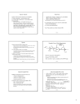
programs outside of the class, whereas private variables cannot be accessed. Public and private labels
are found in the class definition, as shown in Figure 1-3. By defining a concrete interface for a user,
class functions are protected from improper function calls and make the classes simpler to use.
1.4.3Inheritance
Inheritance is another method of reusing code but specifically from an existing class, called a base
class. A class can inherit the member functions and variables of a base class by how the class is
defined. In C++ the declaration of a base class is shown in Figure 1-3. The base class contains one
integer-type member variable, iBaseVar, and one member function called funct1(). The subclass
CSubClass is defined as a subclass of public CBaseClass by using a single colon in the class
definition. By doing this, all of the public member functions and variables of CBaseClass are
automatically inherited by the subclass. Since variable iPrivateVar is a private member variable, it is
not inherited by CSubClass. Functions and variables of the base class are often very general;
therefore, subclasses usually add variables and functions that are more specific to its application.
//Base Class declaration
class CBaseClass
{
public:
int iPublicVar;
//Declare member variables
void funct1(void);
//Declare member functions
private:
int iPrivateVar;
};
class CSubClass:public CBaseClass
{
//Inherits all of the public variables and functions from CBaseClass
//Add more specialized member variables
int iSubClassVar;
//Add more member functions
void funct2(double);
};
Figure 1-3: Class inheritance code example
7
1.4.4Polymorphism
Polymorphism is the ability of a subclass to implement a different version of a member function
inherited from its base class. To keep the interface to the classes uniform, the subclass must have the
same function definition as the base class, however the contents of the function can be different. In
addition, the function must be declared as a public virtual function in the base class. A virtual
function is one that can be overloaded by a subclass. A public function is one that can be accessed
outside of the class. Based on the code segment from Figure 1-3, in order to redefine funct1() in
CSubClass, funct1() must be declared as a virtual function in CBaseClass, as shown in Figure 1-4.
Subclasses must also be declared from public base class. The virtual function in the base class must
be implemented in order for the subclass to inherit it, ie. you can not simply declare the virtual
function.
A pointer to CBaseClass can be used to point to any instance of its subclasses. As shown in Figure
1-5, the compiler will determine which version of the funct1() to use depending on which subclass it
is pointing to. In CSubClass2, funct1() is not redefined, so it that case, the funct1() from the
CBaseClass will be executed.
class CBaseClass
{
public:
//Declare member functions
virtual void funct1(void)
{
printf(“funct1 in CBaseClass\n”);
}
};
class CSubClass1:public CBaseClass
{
//Redefine member function funct1()
void funct1(void)
{
printf(“funct1 in CSubClass1\n”);
}
};
class CSubClass2:public CBaseClass
{
//But does not redefine funct1()
};
Figure 1-4: Polymorphism class declaration example
8
CBaseClass *classPtr;
CSubClass1 subClass1;
CSubClass2 subClass2;
//Pointer to base class object
//subClass1 object
//subClass2 object
//Point classPtr to CSubClass1
classPtr = &subClass1;
classPtr->funct1();
//Calls funct1() defined in CSubClass1
//Point classPtr to CSubClass2
classPtr = &subClass2;
classPtr->funct1();
//Calls funct1() defined in CBaseClass
OUTPUT:
funct1 in CSubClass1
funct1 in CBaseClass
Figure 1-5: Polymorphism function call example
1.4.5Operator Overloading
Operator overloading was used in object-oriented design to override a base class function with a
subclass function of the same name. If the parameters of the base class and subclass functions are
different, then the parameter types used in the function call will determine which version of the
function to use. This property is useful with subclasses that require additional parameters, which
other subclasses, derived from the same base class, do not require.
1.4.6Constructors and Destructors
Constructors and destructors are special member functions that are called on the creation and
destruction of a class object. Referring to Figure 1-5 when the “CSubClass1 subClass1” is called, the
constructor of the subClass1 can be used to perform initialization actions. Destructors are called
when object is deleted using the “delete” command.
9
Chapter 2
Literature Review
2.1 PC-Based Controllers
In the economic world, industries are constantly seeking ways to increase productivity while
decreasing costs. The development of robotics use in automation has greatly facilitated production
gains; however, researchers are constantly looking for more cost effective methods to control robots
for greater efficiency.
In the 1970s, industry of robotic control and automation was dominated by Programmable Logic
Controllers (PLCs).
PLCs were based on “solid-state controllers” as opposed to computer
technology, which was in early development stages at that time. Although the PLCs built the
foundation for automation, they did not take advantage of the developing technology in electronics
and computers. By the 1990s, the solid-state PLCs no longer met the needs of the industry. PLCs
were integrated with micro-processors and became more powerful, but Relay Ladder Logic, the
programming language of PLCs, were not suitable for high-functions required in modern control
systems, such as data communication, diagnostics and data gathering. Engineers found that using
controllers built on Personal Computers (PCs) gave them the ability to attain higher-functions, while
reducing costs [11].
All complex PC-based controllers used for servo control must be able to perform real-time
operations, communicate to peripherals, have high processing power for computations, have the
ability to perform multiple tasks simultaneously and have a method to communicate between those
tasks. Researchers have found many ways to build control systems that fulfill these requirements
such as: using multi-processor computers, building multiple PC and device networks, interfacing with
commercial motion controller cards, using Digital Signal Processing (DSP) boards with Host
computers, and running the controller on single-processor PCs with Real-Time Operating Systems
10
(RTOS). When more than one computer is working together for a common goal, then the system is
called a “distributed” system [12].
2.1.1Distributed Multiprocessor Control Systems
Multi-processor control systems were used for parallel computations of inverse kinematics, dynamics,
trajectory generation and other complex calculations. Many researchers have developed algorithms to
determine which control calculations could be done concurrently, to maximize parallelism and hence
minimize software execution time. Luh et al. [13] used inexpensive processors to increase real-time
computation power by processing control algorithms in parallel based on Newton-Euler formulation.
Kasahara and Narita [14] also used the Newton-Euler method, but were able to actually implement it
on a six-joint robotic arm using a multiprocessing scheduling algorithm. Others have developed
computer architectures for these multiprocessor systems to increase computation efficiency [15], [16],
[17]. These researchers focused on minimizing processing time by splitting-up segments of the
calculations and running them on parallel processors.
Another technique to parallel processing was to assign different tasks to each processor. Kriegman
and Siegel [18] developed a control system for a four-digit Utah-MIT hand shown in Figure 2-1,
which was composed of five microprocessors, one for each of the four fingers plus one processor to
manage all of the tasks. All processors had access to a priority-based multi-bus, where all processes
in the system had equal priority to ensure fair distribution of resources. They also shared dual-ported
RAM, using in high-speed Direct Memory Access (DMA) operations on a VAX system. A servo
loop scheduler was used to manage processes according to the rate of their servo loops. Higher
priority was given to faster servo loops interrupting any slower loops that may have been running,
which had lower priority. For the most part, the fingers were controlled independently and in parallel,
since they were on separate processors, but the managing processor coordinated the fingers to achieve
the desired position in Cartesian space. Inter-processor communication was accomplished with
message passing system that sent standard formatted messages to each processor’s mailboxes.
11
Figure 2-1: Block Diagram of Kriegman and Siegel hand control system [18]
General computer architectures have also been developed to for real-time control. Zheng and Chen
[19] developed a simple, flexible, and modular software structure to manage any multilink systems.
After the user decomposed their multilink system into tasks, they were required to schedule them on
separate processors. Each processor contained a hierarchial executive structure, created by Zheng and
Chen, which took care of task scheduling, interprocess communication and multilevel functions.
Parallel computation of applied torques was also implemented on a separate processor to provide
dynamic control. Other examples of computer architectures for control structures are the CHIMERA
[20] and CONDOR [21].
2.1.2Single-Processor Host and DSP Control Systems
All research previously discussed used distributive systems to attain the computational power
required for real-time systems. Single-processors prior to the 1990s were still too slow compared to
the PCs found today. Instead of having four or five microprocessors to do computations, researchers
have found that using a single-processor computer with a DSP board to be good enough to do the job.
This system is referred to as the Host/DSP system. The host computer is often used to monitor
analyze and collect data from the control system, while the servo control itself is done on the DSP
board using built-in and customized library functions to achieve real-time tasks. Having the DSP
board perform all of the real-time tasks minimizes the overhead in controller computation, and using
multiple DSP boards can allow for concurrent processing. Erol and Altintas [22] developed an Open
12
Real-Time Operating System (ORTS) based on the OSACA system created by Pritschow [23], which
handled and scheduled tasks running on multiple DSP boards in a single Windows NT computer.
Erol and Altintas applied the ORTS for position and force control of a CNC Machine tool.
Disadvantages of Host/DSP architecture are high cost, complex software, and the amount of indepth knowledge required to interface all of the hardware components together.
Research by
Costescu and Loffler [24] showed that there are various advantages to using a single processor-single
host PC for robotic control over Host/DSP systems. The advantages include a decrease in cost, less
hardware, higher flexibility, and better reliability and stability. For these reasons, single-processor
PC-based controllers have recently become highly desirable.
Attempts to create effective real-time controllers for large systems with a single process have been
proven infeasible and inflexible, since such systems require multiple concurrent processes in order to
be efficient. As control systems increase in size, their complexity increases exponentially [25]. Single
processor, PC-based controllers require a stable task-scheduling system to manage concurrent
processes, such as a Real-Time Operating System (RTOS).
2.2 Object-Oriented Software Design in Robotic
Controllers
Software engineering has two main types of architectures: structured programming and objectoriented (OO) programming. Structured programming breaks down a program into its functions or
behaviors as a top-down approach. These programs are simple to design, however they can be
difficult to alter and adapt to new systems. OO design is based on the idea of creating modules of
code, or classes, with generalized functions. This code is then encapsulated so that if one module
changes, the other ones are not affected. Object-oriented software is more difficult to design because
it requires a lot of pre-planning. However, it allows users to modify the code easily as well as reuse
existing for code to minimize development time of new modules. Initially, it was believed that
object-oriented design would cause too much overhead, which is detrimental in real-time control
applications. However, the overhead is negligible [26] and object-oriented control software has been
successfully used in many robotic control applications.
In 1990, Miller and Lennox [27] were one of the first to investigate the use of object-oriented
software design for a robotic controller.
They built the “Robot Independent Programming
13
Environment” (RIPE), a modular software environment that allowed for the quick implementation of
robot systems without dealing with the costly low-level debugging common in structured software
development. The environment itself had four layers: 1) task-level programming, 2) supervisory
control, 3) real-time control and 4) device drivers. The first layer was for planning and simulation.
The second layer was implemented in object-oriented programming based on the physical objects
found in a work cell. It was written in C++ programming language on UNIX operating system.
Using a common general-purpose programming language gave it high portability, and made the code
easier to modify. The third layer dealt with real-time control of devices using a VME-based 68000
family processor running VxWorks, which is compatible with UNIX. The fourth layer contained
device drivers.
OO design has been used for various aspects of robotic controllers. Bagchi and Kawamura used an
object-oriented framework for client and server communication within their distributed robotic
system, ISAC (Intelligenet SoftArm Control) [28].
Barcio and Ramaswamy developed on OO
reactive robotic system built on event-driven state transitions [29]. Robotic control frameworks have
also been created Fernandez and Gonzalez (NEXUS) [30] and Traub and Schraft [31] by applying
OO design.
The most significant research into PC-based robotic controllers relevant to this project was done by
Costescu and Dawson [32] with their development of the QRobot, later renamed QMotor. Unlike
traditional PC-based controllers, QMotor system did not use a DSP for real-time control of hardware
devices, instead all control was accomplished from the PC through the use of a real-time operating
system called QNX Neutrino 4.0. QMotor was composed of four concurrent processes, as shown in
Figure 2-2. QS is the server process used to monitor the MultiQ board used for input/output in the
system. QC is the client process of QS, which contains all of the software that perform control on the
system. QN and QG are additional processes for network communication and the graphical user
interface (GUI) with real-time plots, respectively.
Matlab was used to analyze the data from the
GUI. QG could be run on the same PC as the controller, or connect to it through a network or on a
remote workstation. All these processes were designed using structured programming.
In 2000, Loffler, Chitrakaran and Dawson [33] improved on the QMotor 2.0 to develop an objectoriented QMotor Robotic Toolkit (RTK), now running with QNX Neutrino 6.0. As seen in Figure
2-3, the controller design was based on three sets of classes: Core Classes, Generic Robot Classes and
Specific Robot Classes. These classes built the infrastructure to the controller, including the QMotor
Toolkit, which contained the actual control loop functions. Using an object-oriented design for the
14
controller allows for easy code maintenance, and greatly flexibility.
The QMotor RTK was
successfully tested on a Puma 560 robot arm and a Barret Whole Arm Manipulator (WAM) using
PID control.
Figure 2-2: QMotor 2.0 Hardware/Software Architecture [33]
15
Figure 2-3: Class Hierarchy of QMotor Robotic Toolkit Platform [33]
2.3 Robot Control Structure
The problem of robotic control has been divided into two main categories, trajectory generation (or
planning) and path-control (or tracking). This research focuses more on developing a solid software
infrastructure of the QMARC control system, as opposed to investigating advanced techniques in
trajectory generation and path control. In the current implementation, the QMARC system is capable
of cubic spline trajectory generation and Proportional-Integral-Derivative (PID) control with feedforward velocity and acceleration compensation. More advanced trajectory generation and control
methods can easily be added in the future, as required.
2.3.1Trajectory Generation
A large part of effective motion control for a robotic manipulator is the technique in which the
command path is computed. Obviously, the shortest distance between two points in space is the
straight-line distance, however, generating straight-line positional distance between several knots on
the same path will cause discontinuities in the manipulator velocity and acceleration.
These
discontinuities translate to physical vibrations or jerk on the motors. For pick-and-place operations,
although minimal vibration is tolerable, the overall motion of the manipulator should be as smooth as
possible.
16
One of the earliest forms of robotic trajectory generation was developed by Richard Paul in 1979
[34], whereby straight-line segments with smoothed out transitions at controlled accelerations were
used to connect path knots defined in Cartesian coordinate systems. If two time segments each
required a different constant velocity, then before ending the first time segment a change of velocity
was applied for a time interval of τ. This constant acceleration was then maintained for an additional
τ length of time into the second time segment, hence giving a smooth transition of 2τ between the two
desired velocities. With this trajectory generation method, the path did not actually pass any of the
path knots, except for the end knot. The path, however, could be forced to go through all knots
without causing overshoot at “trajectory extremums” if the velocity at extremums were forced to
zero-velocity. Because all knots were defined in Cartesian space, manipulator link equations were
used to calculate intermediate joint angles to achieve the goal. Taylor [35] improved upon Paul’s
Cartesian technique by developing a method that required the calculation of less intermediate points,
however the computational time of each knot increased.
Thus, he proposed a second interpolation
method implemented in joint space, whereby joint space trajectories were preplanned offline prior to
starting the control loop. Doing this greatly decreased the amount of real-time computations required
but a certain number of path knots had to be known a priori. Taylor presented a method that
produced intermediate points that would guarantee that the straight-line motion stays within
predefined bounds. Both Paul and Taylor used straight-line paths to facilitate compatibility with
conveyor motion.
Because the path segments were not simple straight-line segments, due to the reasons stated earlier,
the path needed to be optimized for minimum time. Luh and Lin [36] developed a minimum time
trajectory generation method using straight-lines with arcs to blend motion between time segments.
The length of these arcs had to be minimized so that the path did not deviate too far from the desired
trajectory.
To perform this optimization, Luh and Lin applied two approaches: a “method of
approximate programming” (MAP), and a “direct approximate programming algorithm” (DAPA).
Doing optimization, in general, requires more computing time. It was found the DAPA converged
and required less computing time than their modified version of MAP.
An alternative to using straight line segments to connect path knots, is to use piece-wise low-order
polynomials. Paul [37] and Finkel [38] proposed trajectory generation using cubic splines. Cubic
splines provided smooth trajectories through path knots despite physical constraints on velocity and
acceleration. To maximize the lifespan of the manipulator, jerk (the rate of change in acceleration)
was also minimized.
Lin et al. [39] used the piece-wise cubic polynomial to interpolate joint
17
trajectories as well. However, to ensure velocity and acceleration continuity, they added two extra
knots to the trajectory that could be freely specified, giving the path enough degrees of freedom for
continuity. To minimize the total travel time of the path, the Nelder and Mead’s flexible polyhedron
search was utilized. All of these earlier methods, only considered the kinematic model of the
manipulator. Dynamic models were later incorporated by Bobrow et al. [40] for more realistic
robotic control.
Trajectory generation and its optimization for both online and offline planning has been a
thoroughly research topic area. Numerous types of splines have been investigated for trajectory
generation, Lin and Chang [41] used X-splines and quartic splines, Dubowsky et al. [42] used the
Bezier, and Bobrow [43] used B-splines, with varying optimization techniques.
2.3.2PID Control Algorithm
Many advanced control algorithms have been developed for robotic control. Classic control methods
include PID feedback control, computed torque method, feed-forward and state-space control. In the
past two decades, growing interest in fuzzy controllers, neural networks and adaptable control
methods has sparked many journal articles on the topic. However, PID controllers have dominated
the control industry of sixty years with more than 95% process control applications [44], and most of
industrial robotic control. PID control stability in rigid robotic arms has been proven by Rocco [45],
based on a robotic model with decoupled linear and nonlinear uncertain components, used for
independent joint control.
The dynamic model of an N degree-of-freedom robotic manipulator is given by a set of Lagrange
equations in the form of:
M (q )q&& + C (q, q& )q& + g (q) = τ
(2-1)
Where, q is the motor joint angle, M(q) is the inertia matrix of the manipulator, C (q, q& ) is the
Coriolis, centrifugal and damping terms, g(q) is the gravitational terms, and τ is a vector of driving
torques acting on the links, which are supplied by motors.
For classic PID control, all motors are treated as decoupled closed loop control systems. The
torque of each individual motor, τm , can be calculated as:
τ m = K P em + K I ∫ em dt + K D e&m
(2-2)
18
Where, em is the position error of the motor, and KP , KI , and KD represents the proportional,
integral and derivative gains of the controller, respectively. Integration and derivation of em are
calculated with respect to time, t [45].
The original method of tuning PID controllers was suggested by Ziegler and Nichols in 1942 [46],
whereby an open loop step response was used to calculate the gains. Ziegler and Nichols presented a
frequency response method and a step response method. Their methods were based on simulating a
large number of different processes and correlating the data to suitable controller gains. The ZieglerNichols tuning method of a PID controller can be summarized as follows [47]:
1. Apply a step input to the system.
2. Increase the proportional gain until sustained oscillations occur, while keeping integral and
derivative gains at zero.
3. When oscillations appear, record the proportional gain value as kU and the period of the
oscillations as tU .
19
4. Three values, kc , Ti and Td , are then computed from the following ratios:
Proportional Gain, kc = 0.6 kU
Integral Time, Ti = 0.5 tU
(2-3)
Derivative Time, Td = 0.125 tU
5. Manually fine-tune the gains by trial-and-error to achieve controller design objective.
Ziegler-Nichols tuning formulas presented in Equation 2-3 are usually implemented in a slightly
different form of the classic PID controller (Equation 2-2). PID implementation for Ziegler-Nichols
is:
dy f ⎞
⎛
1
⎟⎟
u c = k c ⎜⎜ e + ∫ edt + Td
T
dt
i
⎝
⎠
(2-4)
e = yr − y
(2-5)
yf =
1
y
1 + sTd / N
(2-6)
where, uc is the control loop output, y is the process output, and yr is the process command signal.
Although the Ziegler-Nichols tuning method has been very influential, the controller based on
Equation 2-3 provided a closed loop control system with poor robustness [48]. Many researchers
have developed methods to improve Ziegler-Nichols tuning. Cohen and Coon used normalized deadtime to improve controller tuning [49] and Astrom and Hagglund developed a step-response tuning
method based on robust loop-shaping [50].
The time-consuming task of manually tuning the PID controller has also inspired a multitude
papers regarding adaptive and auto-tuning PID controllers such as using pattern recognition [51],
artificial intelligence [52], and fuzzy logic [53].
20
Chapter 3
Design and Implementation
3.1 Overview
The focus of this research was to build a reliable real-time PC-based Multi-Axis Robotic Controller
(QMARC) using QNX operating system for motion control of the Deltabot. QNX is a real-time
operating system, which allows programmers to create efficient multi-process applications. It is a
fundamental tool to the development of the QMARC. The software was designed such that it would
be modular, could easily adapted and would be easy to understand. A modular structure gives the
software the flexibility to be modified to work with new hardware and new features. The overall
structure of the QMARC, as shown in Figure 3-1, has five main software modules, the graphical user
interface (GUI), the controller, the hardware driver, trajectory generator and safety protocols.
Controller settings and initialization is done through the GUI, providing users with a comprehensive
interface to run the controller. The controller itself has access to the trajectory generator, hardware
driver and safety protocols, but only the controller and safety protocols have direct access to the
hardware drivers, which are utilized to control the functionality of the interface card. This card
provides counters to track the encoder position of the motors, analog output lines used to control the
velocity of the DC motors, and digital output lines used to enable the motors through the analog
amplifiers. Six digital input lines are also utilized on the card to interface with the limit switches on
the manipulator. The control loop input is the encoder position read from the counters, and the
controller output is the velocity command signal sent through the analog output lines. A watchdog
timer on the card can also be employed to protect the system in case of the PC crashing. Together,
this structure creates a closed loop control system for position control of the Deltabot.
21
Figure 3-1: QMARC Control Structure
To keep the software modular, the hardware drivers are kept separate from the controller software.
The controller software itself was developed using object-oriented design (OOD), in order to
maximize software modularity and code reusability without sacrificing readability of the code.
Currently, the Deltabot uses the Delta Tau Programmable-Multiaxis-Controller (PMAC) for servo
control. Due to rigidity in the software structure of the PMAC, it was difficult to incorporate
customized control algorithms and trajectory generation techniques.
In order to provide a fair
comparison between the controller developed in this research to the PMAC, the controller was
programmed using PMAC control and spline techniques.
3.2 Hardware Setup
The controller runs on a Dell Optiplex GX110 Pentium III /667MHz computer with a Sensoray 626
encoder card using a QNX Neutrino 6.0 operating system. The encoder card provides up to six 24-bit
22
counters for quadrature decoding, as well as 48 digital input/output channels that have edge-triggered
interrupt capabilities and four analog output channels with 14-bit digital-to-analog conversion (DAC)
providing an output voltage of ±10V. The motor enable signals, as well as the limit switches are
connected to the digital input/output lines of the 626 card with 0V(off) and 5V(on) states. The RS422
protocol encoder signals from all three motors of the DeltaBot are connected to the 626’s dedicated
encoder input channels. The cost of a single 626 card is only $500 US, allowing for the development
of a cost effective control system around a standard personal computer.
3.3 Process Structure of the QMARC
The distributed software system of the controller consists of five concurrent processes, shown in the
ovals in Figure 3-2. These processes are the GUI, Starter, Timer, Controller and Hardware Server.
As their names suggest, the GUI is the QNX Photon Graphical User Interface. On the GUI, the user
can change settings for the QMARC system, and initialize the Starter process. The purpose of the
Starter process is to run (or spawn) the Controller and Hardware Server, and to establish
communication with these processes. The reason that the GUI does not do this directly is because
QNX Photon applications do not have the same communication channels as regular QNX programs.
It is simpler for the GUI to spawn the Starter process to handle the process communication. The
Timer process is a real-time interrupt that keeps track of the system clock initiated from the
Controller process. The Timer sends the Controller messages at a fixed sampling rate. When the
Controller receives a Timer message, it sends a message to the Hardware Server requesting
information about the current position of the motor. Using the data about the motor, the Controller
performs its control algorithm and sends a second message to the Hardware server providing it with
the command for the motor. The Hardware Server is a separate process that manages all data to and
from the encoder card as well as analog/digital inputs and outputs and safety features. This process is
always waiting for the Controller to send it messages. When the Hardware Server has completed its
task, it replies to the Controller, freeing it from its blocked state.
23
Figure 3-2: QMARC Process Communication Structure
Once the Controller runs to completion, it ends the Timer and sends a message to the Hardware
Server telling it to exit. Before exiting, both the Hardware Server and the Controller sends a message
to the Starter program telling it to end as well. Thus all processes exit and the user can return to the
GUI process to run the controller again.
The messages sent between the processes only occur in one direction, with replies returning in the
opposite direction. The Starter sends replies to the Controller and Hardware Server and the Hardware
Server replies to the Controller, however the Timer does not require a reply. Using this client-server
communication network prevents deadlock, which is a serious problem in multi-process systems.
The Hardware Server runs at the highest priority, next is the Timer and then the Controller. Setting
important processes to high priorities ensures that they execute without interruption by low-priority
processes. The priority of the Hardware Server is 60, whereas the Controller and Timer are at a
priority of 50. The Starter runs at the lowest priority of 30.
Using the distributed software structure with this hardware-communication setup allows for fast,
efficient real-time control of the motor.
Because only the Hardware server deals with direct
protocols to the 626 Encoder card, the hardware is effectively decoupled from the software system.
This means that changing the hardware will not affect the controller software, and just the Hardware
Server needs to be updated.
24
3.3.1QNX Message-Handling Functions
QNX has many message handling functions that can be used for ease of communication between
processes. Before sending a message to a process, the structure of the message must be defined and
communication connection must be established between the processes.
The message structure can vary between applications depending on the need of the client and
servers. For this research, four different fields were required in the message, defined by structure
called ClientMessageT, as shown in Figure 3-3. The first field is an integer, iMsgType, representing
the message type, or what kind of task it wants performed by the server. The second field is
fMsgData, a floating-point array containing data transferring between the client and server processes.
The third field is an integer array containing initialization data used to establish communication
between the client and server processes. The fourth field is an integer representing the status of the
server, iStatus, used to communicate success or hardware failures. The fMsgData and iInitData
arrays are defined to be the size of the maximum number of motors in the system, providing enough
room to contain data for every motor in a single message. For the Deltabot, NUM_MOTOR_MAX is
equal to three.
// message structure
typedef struct
{
int
iMsgType;
float fMsgData[NUM_MOTOR_MAX];
int
iInitData[NUM_MOTOR_MAX];
int
iStatus;
}ClientMessageT;
//Message Type
//Floating-Point Data
//Initialization Data
//Status of hardware
Figure 3-3: Message Structure for Client-Server Communication
To establish communication between the client and server processes, the server needs to provide the
client with its process id and channel id numbers. The process id number can be retrieved within any
process by calling the getpid() function, and the channel id can be created by calling ChannelCreate().
With this information, the client can establish a connection to the server by calling ConnectAttach().
ConnectAttach() returns a connection id number, which is then used to send messages to the server.
Sample code of how to do this is shown in Figure 3-4. Messages are sent from the client using the
MsgSend() function, and is received by the server with the MsgReceive() function. MsgReply() is
used to send a reply message to the client after the server is finished. It is important to plan how the
25
server process id and channel id will be sent to client processes, so that they can establish
communication to the server.
#define MT_ENABLE_MOTORS
#define NO_ERR
30
0
//Message Type
ClientMessageT outmsg, replymsg, inmsg;
/* In server process */
Process_id = getpid();
Channel_id = ChannelCreate(0);
//Get process id
//Create a communication channel
//Server loops infinitely processing messages
while (1)
{
//get the message and print it
rcvid = MsgReceive (chid, &inMsg, sizeof (ClientMessageT), NULL);
//perform function to enable motors
.
.
.
//Reply to client when completed
outMsg.iStatus = NO_ERR;
MsgReply (rcvid, EOK, &outMsg, sizeof (ClientMessageT));
}
.
.
.
/* In client process*/
connection_id = ConnectAttach (0, process_id, channel_id, 0 , 0);
outmsg.iMsgType = MT_ENABLE_MOTORS;
MsgSend(connection_id,
outmsg,
sizeof(ClientMessageT));
sizeof(ClientMessageT),
replymsg,
Figure 3-4: Example code for client-server communication and message-handling
After the client process calls MsgSend(), the client process will stop running (or be in blocked state)
until the it receives a reply message from the server call to MsgReply(). On the server side, the server
is blocked until it receives a message from the client with MsgReceive(). When a process is in a
blocked state, other processes are allowed to run. By setting the client and server to high priorities, it
can be ensured that they can continue to run again as soon as they are unblocked. For the QMARC,
all message types are defined in the MsgType.h header file located in the Include folder of the main
directory of the QMARC system.
26
3.4 Design of the Controller Console
Programming a Graphical User Interface (GUI) on the QNX operating system is very similar to
Microsoft Visual C++ development. Using the QNX Momentics Software Development suite, GUIs
can be creating with predefined widgets, such as buttons, integer edit boxes, floating point edit boxes,
combo boxes, and labels available in the Photon Application Builder.
Photon operates on the
principle that any event caused by moving or clicking the GUI, will send a message to the main
Photon message loop. It is up to the programmer to write specific functions to handle desired events.
For example, when a button is clicked on by the mouse an “arm” message is created. By writing a
callback function for the “arm” message, the programmer can specify what actions are taken when the
button is clicked. Because Photon has special messages that it uses to process actions on the GUI,
regular QNX message-handling described in section 3.3.1 can not be done. Instead, special Photon
message channels must be setup to establish communication. In the QMARC system, the GUI will be
referred to as Controller Console and its purpose is to initialize the controller. Since the Controller
Console is not updated by information from other processes, it was not necessary to setup Photon
communication channels. Instead, the GUI spawns Starter, a QNX process that handles all of the
communication for it.
The layout of the Controller Console is shown in Figure 3-5, depicts the five main sections of the
GUI. The first section is “Controller General Settings”, which allows user to set the number of
motors to be controlled, the servo loop period and the home position measured from the top limit
switch in counts. The servo loop period is restricted to periods of at least 300μs and must be an even
multiple of 100. The second section has the “Trajectory Generation” settings. This section allows the
user to select the method of trajectory generation to use and select the file location where the path
knots are stored. The third section is the “Step Motor” settings. When tuning the PID controller, a
step input is generally used. The size (in counts) and duration (in seconds) for the step input can be
specified from the GUI. To run the step, the user must click on the “Step Motor Now” button. Note,
that doing this will step all motors specified in the first section of the GUI. The fourth section is the
“Controller Gains” settings. It allows the user to specify gains used for the PID controller with feedforward velocity and acceleration compensation and notch filter for the number of motors specified.
Although there are entries for four motors, the maximum number of motors allowable on the Deltabot
is currently three. The edit boxes for motor gains, which are not being used will be disabled on the
GUI whenever the user updates the “Number of motors” edit box. The sixth section is “Data Gather
27
Settings”. Here, the user can specify the frequency to collect data, the file location to log the data,
and what fields to collect. The frequency of gather data is a function of the servo loop, it can be set to
gather data every servo loop, every other servo loop etc. There are four different fields that can be
collected: time of the sample, DAC output to the motors, the command position and the actual
position of the motor, measured in counts. The data is output in a Matlab data file and should have a
“.m” extension. Writing the data to a Matlab file allows the user to graph to data more easily on a
computer with a Microsoft Windows platform. Currently, graphing features are not used on the QNX
computer.
All controller settings on the Controller Console, except for the “Step Motor” settings are saved to
a settings.txt file, located in the directory of the Console program, before exiting the program.
Whenever the GUI is started, the controller settings are retrieved from the file and loaded onto the
GUI.
After the controller settings are entered, the user can click on the “Home Robot” button to run the
homing sequence of the robot, or click on the “Start Controller” button to run the robot with the
trajectory generator specified. The “Cancel” button is closes the GUI without saving changes to the
settings file, whereas the “Exit” button will save the settings before exiting. Whenever the “Step
Motor Now” button, “Home Robot” button or “Start Controller” button is clicked on, the data from
the GUI is saved to the settings file, and the Starter process is spawn from the GUI. To determine
which button was pressed, the GUI sends a message type flag to the Starter process. This information
is then passed along to the Controller process so that it can start up in the appropriate controller mode.
While tuning the controller, it is often useful to know the accumulated absolute position error of the
motors. This statistical data is displayed on the same terminal where the user runs the Controller
Console program. All error messages from the Hardware Server or the Controller will be displayed
on this terminal as well.
28
Figure 3-5: QMARC Photon Graphical User Interface (GUI)
3.5 Design of the Starter Process
The purpose of the Starter program is to be a gateway between the Controller Console and the
Controller and Hardware Server processes. As mentioned in section 3.4, the Controller Console does
not use the same message channels as the QNX processes, making communication more difficult.
However, since the console does not need to be updated by any other process, the GUI only needs to
do one-way communication. As shown in Figure 3-6, when a button (other than the Exit button) is
pressed on the console, the Starter process is spawned from the GUI passing along information about
29
which button was pressed, using the spawnl() function. The Starter program reads these values in as
string arguments and converts them to integer or floating-point values. Starter than spawns the
Hardware Server and Controller processes using spawnl() passing them its channel id number.
Starter’s channel id is used by the Hardware Server and the Controller to connect it. The connection
allows the Starter to know if the spawnl() was successful. When Hardware Server is spawn it sends a
message to the Starter to inform it that the spawnl() call was successful, and it also sends back its own
Process ID and Channel ID numbers. These ID numbers are then passed on the Controller process by
the Starter, so that the Controller can establish direct communication with the Hardware Server. If
the “Step Motor Now” button was pressed on the GUI, then the step size and duration are passed to
the Starter program as arguments in spawnl() and passed to the Controller process in the reply
message. Starter then waits for a message from the Hardware Server and the Controller indicating
that it is done. Once it receives messages from both processes, the Starter program exits. Keeping
the Starter process running ensures that any error messages from the child processes will be displayed
on the terminal window. If the Starter process exits immediately after spawning the processes, the
error messages and statistical data will be lost, unless it is output to file.
30
Button pressed on Controller Console
START
Retrieve GUI data from spawnl() arguments
Create a channel for message communication
Spawn Hardware Server passing it the channel id
Block process, waiting for a message to be
received from Hardware Server using the
MsgReceive() command
No
Has
a message been
received?
Yes
Send a reply to Hardware Server
Spawn Controller process passing it the
channel id of Starter
Block process, waiting for a message to be
received from Controller using the
MsgReceive() command
No
Has
a message been
received?
Yes
Send reply to Controller with GUI button data and
Hardware Server’s Process ID and Channel ID
Block process, waiting for “Done” messages
from the Hardware Server and Controller
No
Messages
received?
Yes
END
Figure 3-6: Flow Chart of Starter Process
31
3.6 Design of the Hardware Server
The Hardware Server is a process initialized from the Starter process, and terminated by a message
from the Controller process.
This server receives messages regarding input and output to the
Sensoray 626 Encoder card. It performs all hardware input and output, and monitors limit switches
using an edge-triggered interrupt line built into the interface card. The Hardware Server runs in a
semi-infinite loop blocked by the operating system on a MsgReceive() command until it receives a
message from the Controller.
When a message is received, the Hardware Server unblocks,
determines the type of message that was sent to it using the integer field, iMsgType, in the message
and then performs the appropriate actions. After the action is completed, the Hardware Server sends
a reply message back to the Controller along with the status of its actions, and then continues back to
the beginning of the message loop. The server handles twelve different messages:
1. Retrieve the encoder counter values for all motors.
2. Send DAC output for all motors.
3. Retrieve the encoder counter value for a single, specified motor.
4. Send DAC output for a single, specified motor.
5. Enable a single, specified motor.
6. Disable a single, specified motor
7. Disable all motors
8. Reset encoder counter to “zero” value.
9. Enable interrupts to monitor hardware safety features.
10. Disable interrupts to monitor hardware safety features.
11. Clear safety status flag.
12. Exit Hardware Server
A safety status flag is used to monitor the errors in the Hardware Server. If the limit switches are
tripped, encoder overflow occurs, or an unrecognized message is detected, the status flag is set and
sent back to the Controller in the reply message.
Messages are processed in order of time-critical
importance. Messages related to retrieving encoder positions and sending DAC output is checked
first in the message loop because they are used in a real-time control loop by the Controller. Single
motor functions are kept separate from functions that apply to all motors. Single motor functions are
predominately used in homing procedures. Functions concerning all motors are used for time-critical
32
control loops, since sending a single message for each motor can be time consuming. All data passed
in the messages are stored in the fMsgData array contained in the message structure.
The Hardware Server was written specifically for the Sensoray 626 encoder card using the
Sensoray QNX library.
Hardware protocols are kept separate from the Controller so that the
Controller is decoupled from the equipment used in the application. This means that if new hardware
is purchased, only the Hardware Server will have to be rewritten, saving both time and money.
When the Hardware Server is initially started from the Controller Console, it connects to the Starter
and sends it a message with its process id and channel id number. Through the Starter, the process id
and channel id of the Hardware Server is passed to the Controller. As shown in Figure 3-7, the
Hardware Server then runs in a semi-infinite loop processing messages received from the Controller
and performing calls to the Sensoray QNX library. When the server receives an exit message from
the Controller indicating that the Controller is complete, the Hardware Server sends a “Done”
message to the Starter program and then exits. Safety protocols and homing procedures will be
covered in section 3.10.
START
Initialize the 626 Encoder Card
Block process, waiting for a message to be
received using the MsgReceive() command
Has
a message been
received?
No
Yes
Determine what type of message was received
Perform actions required
Was
it an “Exit”
message?
No
Yes
Send “Done” message to Starter Process
END
Figure 3-7: Flow-chart for Hardware Server
33
3.7 Design of the Timer
The Timer consists of a software interrupt handler, using the timer interrupt number 0 built into QNX
Neutrino 6.0. The period of the timer interrupt is determined by calling ClockPeriod(), a QNX
function called from the setupTimer() function in the MultiAxisRobot class. A global timer event
variable, timevent, is attached to the timer interrupt and then linked to an interrupt service routine
(ISR), as shown in Figure 3-8. For the QMARC, the interrupt handler is set for a period of 100 μs. In
the ISR, a global variable is used to keep track of the number of times the timer interrupt has
occurred. This variable, timctr, must be declared as volatile. When the counter equals the servo
interrupt time of the servo loop, then the ISR returns the timer event, so that the Controller process
unblocks the InterruptWait() command in the servo loop.
struct sigevent timevent;
volatile unsigned timctr;
//Timer Event
//Timer for counter
//ISR - Interrupt Service Routine
//Handles the timer ClockPeriod() interrupts
const struct sigevent *handler(void *area, int id)
{
//Clock runs by period set by ClockPeriod()
if(++timctr == iServoIntRnd)
{
timctr=0;
return(&timevent);
}
else
return(NULL);
}
//Set the timer interrupt according to ClockPeriod(), interrupt 0
int MultiaxisRobot::setupTimer(void)
{
struct _clockperiod clkper;
//Set the Clock Period to minimum value of 100 microseconds
clkper.nsec = 100000;
clkper.fract = 0;
ClockPeriod(CLOCK_REALTIME,&clkper,NULL,0);
ThreadCtl(_NTO_TCTL_IO,0);
timevent.sigev_notify=SIGEV_INTR;
//Request I/O privity
//Initialize event structure
//Attach ISR vector, interrupt 0 is clock interrupt
timid=InterruptAttach(SYSPAGE_ENTRY(qtime)->intr,&handler,NULL,0,0);
return 0;
}
Figure 3-8: Code for Timer ISR and Setup Procedure
34
3.8 Design of the Controller
The Controller is the heart of the QMARC system. It consists of the control algorithm, trajectory
generation, safety procedures, timing and hardware message handling in closed control-loop.
Objectives of the Controller design were to create a general software structure that had high
flexibility, expandability, and was easy to follow, update and understand. High flexibility allows for
expansions in the software such as applying different control algorithms and trajectory generation
techniques. Hardware changes such as the incorporation of a vision system and different endeffectors, motor drives and manipulators should also be possible with minimal change to the existing
software. To build a flexible system, the software structure needs to be modular. A modular program
keeps segments of code encapsulated, such that a change in one component of the software will not
adversely affect other areas. In software engineering, a technique called Object-Oriented design is
used to achieve this goal [10].
The object-oriented structure used for this project was developed based on research by Loffler et al.
[33].
As shown in Figure 3-9, the controller was organized into Base Classes and Specific
Subclasses. The Base Classes are modules providing general functions and properties commonly
found in a robotic motion controller. Five base classes were created for this motion controller:
CObject, CManipulator, CGripper, CTrajGenerator, and CServoCtrl. All Base Classes are preceded
with a “C” to distinguish them for Specific Subclasses.
The Base Classes are divided into two groups: physical classes and functional classes. Physical
classes are based on physical hardware used in the motion controller, whereas functional classes deal
with the mathematical aspects of the controller. On the hardware side, there is the CObject class.
This class contains all properties common to any physical object, such as a universal system timer,
servo loop period etc.
CManipulator and CGripper are classes for manipulators and grippers,
respectively, and are subclasses of CObject. Being a subclass means that it inherits all of the parent
class’ public properties and functions.
If additional hardware is required, then new subclasses can
be made from CObject. The remaining two base classes: CTrajGenerator and CServoCtrl, contain the
operations and calculations required for trajectory generation and servo control, respectively. By
default, the CTrajGenerator produces a constant trajectory used for Step Input. Using the five base
classes defined above, Specific Subclasses can be derived that are specific to the controller
application.
All base classes were designed to maximize reusable code by a specific subclass.
35
The motion controller in this research was designed for control of the Deltabot. Key functions such
as performing the control loop are defined in the MultiaxisRobot class, a subclass of the
CManipulator base class. The MultiaxisRobot class also contains the communication protocols to the
Hardware Server and the Timer used for the control loop. The control algorithm implemented on the
manipulator was PID control with Velocity and Acceleration Feed-Forward compensation, which is
contained in the PIDffCtrl class derived from the CServoCtrl base class. Details on this control
algorithm are covered in Section 3.11. In addition, two different methods of trajectory generation
were implemented in this controller: offline cubic spline and online Position-Velocity-Time (PVT)
trajectory generation.
These techniques were separated into two different classes named
CubSplineTrajGen and PVTOnlineTrajGen. Trajectory generation is used to determine the command
position for each time instance of the servo loop. Details on these algorithms are covered in Section
3.12. In addition, it should be noted that both the control and trajectory generation algorithms were
implemented from the PMAC model, to facilitate the comparisons between the two controllers. The
control of the gripper was not necessary in this research; therefore CGripper does not have a specific
subclass.
Base Classes
CObject
CManipulator
CGripper
CTrajGenerator
CServoCtrl
MultiaxisRobot
CubSplineTrajGen
PVTTrajGen
PIDffCtrl
Specific Subclasses
Figure 3-9: Class structure of robotic motion controller
3.8.1.1
Detailed Base Class Descriptions
This section will cover the detailed software description of each base class: CObject, CManipulator,
CGripper, CTrajGenerator and CServoCtrl. Not all base classes are fully implemented but are still
presented here to demonstrate the full software infrastructure for future research development.
36
As a standard naming convention for all member variables, variables with an “i” prefix represents
an integer data type and “f” represents a floating point number. Integers are two-byte signed values
ranging from –32768 to 32767. Floating-point numbers are four bytes long and range from -3.4 X
10-38 to 3.4 X 1038.
Base classes: CObject, CTrajGenerator and CServoCtrl all contain a floating-point variable,
fServoInt used to specific the period of the servo interrupt in seconds. This variable is defined by
calling the init() function in each base class. This init() function is declared as virtual so that it can be
overloaded by subclasses if necessary.
3.8.1.1.1
CObject Class Description
The CObject class contains a member variable for the servo interrupt period, fServoInt. It also
contains the init() function that sets this variable and converts it from microseconds to seconds.
3.8.1.1.2
CManipulator Class Description
The CManipulator Class has three member variables: iNumMotors, iHome and fCurPos, which
represents the number of motors in the manipulator, the home position of each motor measured in
counts and the current position of each motor in counts.
Virtual functions are also defined for the control loop (ctrlLoop()) and to setup the timer
(setTimer()). These functions are implemented in the subclass level. Only empty functions are
provided here to ensure the polymorphism can be applied to future subclasses of CManipulator.
3.8.1.1.3
CGripper Class Description
The CGripper class currently does not contain any member variables or function. It is added as a
demonstration of how the CObject class can be used and is reserved for future research development.
3.8.1.1.4
CTrajGenerator Class Description
Command positions are created for servo control via trajectory generation. CTrajGenerator class
contains four member variables: fServoInt represents the servo interrupt period, fPosQueue represents
a pointer to the position queue, iPosCurPtr indicates the index of the current position to read
command values, and iPosQueueCtr gives the total size of the queue. All of these variables are used
for the collection of command positions at each time instance of the servo control.
For offline
trajectory generation, these position values are calculated prior to starting the control loop. The size
of the position queue is dynamically allocated in real-time based on the total time length of the
manipulator motion, as well as the desired servo control clock frequency.
37
Dynamic memory
allocation is performed by calling member function setPosQueue(), giving it the size of the desired
queue. Queue size is calculated using the following equation:
Position queue size = (total time of move / servo interrupt period) + 1
Member function getCurPosQueue() is used to retrieve the current command position from the
position queue.
In CTrajGenerator there are two sets of virtual member functions for: online and offline trajectory
generation. Online trajectory generation requires separate functions for interpolating between two
knots (interpPoint()) , calculation path segment coefficients (calcCoeff()) and to retrieve real-time
data (readData()). Offline trajectory generation combines all computations in one simple function
called to calcPath(). All of these functions are redefined at the subclass level. The default trajectory
implemented in calcPath() is an ideal step input, with a step size and duration defined by the user in
the Controller Console.
3.8.1.1.5
CServoCtrl Class Description
The control algorithm for the motion controller is contained in the CServoCtrl base class. CServoCtrl
contains one member variable for the new DAC output, fDACOut, and two member functions to set
the gains of the controller (setGain()) and the control computation itself called ctrlCalc(). Both
setGain() and ctrlCalc() are empty in this base class and are reserved for implementation in its
subclasses.
3.8.1.2
Detailed Specific Subclass Descriptions
The Specific Subclasses are written for a specific application of the QMARC. All subclasses are
derived from one of the five base classes described in Section 3.8.1.1. For motion control, four
specific subclasses are used: MultiaxisRobot, CubSplineTrajGen, PVTTrajGen and PIDffCtrl.
Variable data type naming conventions are identical to those described for the Base Classes.
3.8.1.2.1
MultiaxisRobot Class Description
The MultiaxisRobot Class is derived from the CManipulator base class, and is primarily used for the
communication to the Hardware Server, to initialize and monitor the Timer of the controller, perform
the control loop, and handle safety protocols involved with hardware and software faults.
There are two member variables in this class used for communication: the connection ID (iCoid), is
used to communicate to the Hardware Server, and iTimid holds the process id for communication to
38
the Timer.
Functions sendServerMsg() is used to send messages to the Hardware Server,
faultHandler() is used to handle fault messages received from the Hardware Server, and setupTimer()
is used to initialize and setup the Timer.
The settings for gathering data are summarized in three member variables: outFilePtr is a file
pointer to the output file, iDataGatherFreq gives the frequency to gather data in the servo loop, and
iDataGatherFlags contains the bit flags indicating the fields to gather data from. The options for data
collection during the servo loop are: time, DAC output, command position and actual position. The
logged data is output to a Matlab file by calling the outputDataFile() member function.
In order to read knots that define the desired manipulator path, two variables are used:
iCurQueuePtr representing the position of the circular queue with knot data and bQueueEOF flag
used to indicate the end of the queue. This circular queue is an array of the position-velocity-time
(PVT) structure type with a length of 10, which is declared globally. It is used only for online
trajectory generation in the member function readFile() of the PVTOnlineTrajGen class.
All of these member variables and functions covered thus far are private and can only be accessed
within the class. Another private member function called homeCtrlLoop() is a special control loop
used to home the motors.
Public member functions include initiating communication to the Hardware Server and setting the
servo interrupt period in init(), ending communication in close(), setting the home position of all
motors in setHomePos(), setting the “zero” encoder positions for the motors in zeroMotorPos() and
the performing
the control loop.
Depending on the value of member variable indicating the
trajectory generation mode (iTrajGenMode), ctrlLoop() is called for offline trajectory generation,
whereas ctrlLoopOnlineTrajGen() is called for online trajectory generation. Both ctrlLoop() and
ctrlLoopOnlineTrajGen() require pointers to CTrajGenerator and CServoCtrl objects to perform the
control loop, however online trajectory generation also requires a pointer to a data file containing
information on path knots. Since the control loop functions use base class pointers as inputs, they
accept any subclasses of that base class as well. This is possible due to the polymorphic nature of
object-oriented software design. By setting the base class pointers to the appropriate subclass, the
trajectory generation and control algorithm can be altered without modifying the member function.
The calcPath() function must always be called prior to calling the ctrlLoop() function. Since
ctrlLoop() assumes that the position queue for the command path has already been calculated. The
algorithm used for this control loop is shown in Figure 3-10. Basically, the program determines the
length of the position queue by reading the CTrajGenerator member variable iPosQueueCtr, and then
39
loops around waiting for an interrupt from the Timer. It then extracts the current command position
using getCurPosQueue() and calculates the new DAC output by calling ctrlCalc() in CServoCtrl.
Sending messages between processes take considerable time, so to minimize time in the control loop
a single message is sent to the Hardware Server to retrieve all motor positions and to send all motors
their new DAC output signal. All statistical data is saved to a buffer array during the motion, and is
output to a Matlab file after the move is completed. The motors and safety features are automatically
enabled before the move and disabled after the move is done.
The algorithm for the control loop used in online trajectory generation (ctrlLoopOnlineTrajGen())
is shown in Figure 3-11. This control loop is very similar to ctrlLoop() used in offline trajectory
generation, except the total time of the move is marked by the end of the data file containing the PVT
knots for trajectory generation. The readFile() function in the MultiaxisRobot class is used to read
data from the PVT data file and store knots into a circular queue. The first time readFile() is called,
the first three knots in the path are read, then every successive call reads two knots. This means that
in order to do PVT online trajectory generation at least three points on the manipulator path must be
known a priori. Instead of reading in three points, the function can be easily modified to read in only
two, however this is left for future research. The PVTOnlineTrajGen class has its own readData()
function used to copy knot points from the circular queue to a small array located within the class
memory. After reading the initial path knot from the queue, the program enters a loop where it first
reads in a point representing the end of the time segment, calculates the coefficients of the cubic
spline between the two knots and then loops through waiting for the interrupt and interpolating
command positions, doing control, at each time instance within that segment. When the time segment
covered by the two knots is finished, the function reads another knot from the circular queue, until the
end flag in the circular queue is found. This end flag signifies an end of file, which terminates the
control loop and outputs data to file.
40
START
Initialize variables
Get length of command position
queue from CTrajGenerator
Send message to Hardware Server
to enable all motors.
Get start time of control loop
Is
i < length of
position queue?
No
Yes
Wait for Timer interrupt
Send message to Hardware Server to retrieve
encoder positions for all motors
i = i+1
For
each
motor
Calculate current command position by calling
getCmdPos() inCTrajGenerator
Calculate new feedrate by calling
ctrlCalc() in CServoCtrl
Send feedrate in message to Hardware Server
to output command signal to all motors
Save current time, actual and command
position data to buffer array.
Output error message if control interval is > 20us
of the desired period of the controller.
Send message of Hardware Server
to disable all motors
Output data in buffer array to a Matlab file
END
Figure 3-10: Flow-chart of algorithm for offline trajectory generation control loop, ctrlLoop()
41
START
Initialize variables
Read data for initial knot for each motor in
CTrajGenerator by calling readData()
Send message to Hardware Server
to enable all motors.
Get start time of control loop
Read in data point for end of time segment by calling readData()
and calculate path coefficients by calling calcCoeff() in CTrajGenerator
Is
it the end of
the data file?
Yes
No
Calculate run time of controller and time shift
factor for current time segment.
Wait for Timer interrupt
Send message to Hardware Server to retrieve
encoder positions for all motors
For
each
motor
Calculate current command position
through CTrajGenerator by calling interpPoint()
Calculate new feedrate by calling
ctrlCalc() in CServoCtrl
Send feedrate in message to Hardware Server
to output command signal to all motors
Save current time, actual and command
position data to buffer array.
Output error message if control interval is > 20us
of the desired period of the controller.
Is
run time
within current time
segment
Yes
No
Send message of Hardware Server
to disable all motors
Output data in buffer array to a Matlab file
END
Figure 3-11: Flow-chart of algorithm for online trajectory generation control loop,
ctrlLoopOnlineTraj()
42
3.8.1.2.2
CubSplineTrajGen Class Description
The cubic spline offline trajectory generation class CubSplineTrajGen is derived from the
CTrajGenerator base class. CubSplineTrajGen has two private member functions: getAcceleration(),
which calculates the acceleration of each knot so that the acceleration, velocity and position of the
trajectory is continuous and interpPoint(), which interpolates the position for any point in time.
InterpPoint() is declared as a virtual function in the base class CTrajGenerator, however, for offline
trajectory generation overloads the operators to make the function suitable for offline computation.
Both interpPoint and getAcceleration() are used by calcPath(), which is the only public member
function of this class. CalcPath() calculates the cubic spline path for any set of non-uniformly spaced
knots, and produces a full position queue ready for the control loop. The mathematics of this class
are covered in Section 3.12.1.
3.8.1.2.3
PVTOnlineTrajGen Class Description
The Position-Velocity-Time (PVT) trajectory generation class PVTOnlineTrajGen is derived from the
CTrajGenerator base class. There are eight member variables in this class: iCurKnotPtr is the current
position on the circular queue used by the trajectory generator, the coefficients fA, fB, fC and fD of
the cubic spline polynomial equation, and arrays for two time instances of position, velocity and time
in variables fP, fV, and fT. Public member functions include: a constructor used to initialize class
variables, readData() used to read PVT values from circular queue, calcCoeff() uses the PVT knots to
calculate the fA, fB, fC, and fD coefficients of the cubic polynomial for the current time segment,
interpPoint() is used to interpolate the position within a spline segment, and saveDataInstance() used
to move array values from the current time instance to previous time instance in fP, fV and fT. The
mathematical details of this class are covered in Section 3.12.2.
3.8.1.2.4
PIDffCtrl Class Description
The PID control with feed-forward acceleration and velocity algorithm with a notch filter is
implemented in the PIDffCtrl class. This class is derived from the CServoCtrl base class and has five
private member variables representing the gains of the controller, which can be set by calling the
public setGain() member function. The gains are: portional gain (fPGain), integral gain (fIGain),
derivative gain (fDGain), feed-forward velocity gain (fKvff), and acceleration gain (fKaff). Two
private arrays are used to store the coefficients of the notch filter. Array fNcoeff stores the
coefficients for the numerator and fDcoeff stores the coefficients of the denominator, covered in
Section 3.11.1 of the notch filter.
43
In addition, this class has five member variables used to store a few time instances of intermediate
variables used for the control calculation, these are: position error (ferror), integral error (fIntError),
command velocity (fCmdVel), command position (fCmdPos), and actual position (fActPos). To
calculate the feedrate for the motors, the controller calls the ctrlCalc() function. The init() is first
called to initialize all private member variables. The mathematical details of this control algorithm
are covered in Section 3.11.
3.9 Running the Controller
Before starting the control loop, the Controller is initialized by the Starter process, receiving the
process id and channel id of the Hardware Server. The Controller then reads the settings.txt data file
written by the Controller Console and saves the settings into the memory. It then processes the reply
message type from the Starter to determine which button on the GUI was pressed. Depending on the
button type, three different functions are called homeRobot(), stepMotor() or initCtrller(). These
three functions call and initialize the class functions.
3.10 Safety Features
Applying the QMARC to a robotic manipulator required the implementation of safety measures to
ensure that the robot arm and the motors of the Deltabot were not damaged if the control law became
unstable. Safety protocols monitoring motor positions with limit switches, software limits of the
encoder counters, and following error of the controller were developed.
3.10.1
Hardware Limit Switches
The DeltaBot uses two proximity limit switches to indicate maximum and minimum angles allowed
by the arms connected to each of the three motors. The QMARC uses six digital input channels to
monitor the limit switches via hardware interrupts initialized from the Hardware Server. When a
limit switch is tripped, the server determines which limit switch it was and sets a status flag for that
motor. As a result all limit switch interrupts are temporarily disabled. When the Controller process
requests information from the Hardware Server during the servo control loop, the server informs the
controller process that the limit switch has been tripped using the iStatus field in the message. When
44
the Controller receives a non-zero status flag, the Controller exits the control loop and enters the fault
handler function, faultHandler() in the MultiaxisRobot class.
The faultHandler() immediately
disables all motors and outputs an error message to the terminal.
3.10.1.1
Robot Homing Procedure
During homing, the limit switches are used to set the home position of each motor of the manipulator.
This is activated by pressing the “Home Robot” button on the GUI. The homing is done through the
setHomePos() function in the MultiaxisRobot class.
Function setHomePos() calls the
homeCtrlLoop() function, to move the robot arm at a constant velocity up to the top limit switch.
When the Hardware Server finds the top limit switch, it sets the status flags and informs the
Controller of the status of the limit switch at the next hardware request. The control loop will end
immediately and return to the setHomePos() function in MultiAxisRobot class.
The homing
subroutine will move the motor down slowly. At every sampling interval it will check to see if the
status of the limit switch triggered has changed, to make sure that the motor is no longer outside of its
boundaries. If the motor does not clear the limit switch within 10 counts, then a fatal error could have
occurred, so all motors are disabled as a safety measure. If the motor clears the limit switch within 10
counts successfully, then robot arm moves to the home distance set by the Controller Console. The
motor encoder counter is set to “zero” value. The entire process is repeated for each motor one-byone.
To maintain the client-server communication hierarchy, the Hardware Server cannot send a
message to the controller process directly when it knows that a limit switch has been tripped. In the
worse case scenario, the limit switch would occur immediately after the client receives a response
from the Hardware Server. This means that it would take one sampling interval for the appropriate
actions to be taken by the Controller. For our application a delay of one servo interrupt period is
tolerable.
3.10.2
Software Position Limits
The counters used to measure the position of the motor encoder signals are located on the Sensoray
626 encoder card. These counters have 24-bit resolution, with a range from 0 to 16777216. At the
end of the homing sequence described in section 3.10.1.1, the counters are set to “zero”. This “zero”
value is actually 8388608, a value in the mid-range of the counter. An addition 32-bit signed long
software counter is used for every motor, which is set to zero by the zeroHomPos() function in the
45
MultiAxisRobot class. Every time the hardware counter is read, the Hardware Server calculates the
change in the counter from the previous time instance, and adds the difference in counts to the
software counter. The software counter ranges from -2,147,483,648 to 2,147,483,648. Using a a
variable to store the counter value prevents the problem of counter overflow, which may occur in
robot motion using a hardware counter. Any hardware counter overflow that does occur is handled
by the calculation of the software counter.
3.10.3
Following Error Limit
When a controller becomes unstable, the accumulated following error of the position can blow up
dramatically. To ensure that controller instability does not damage the manipulator, a software limit
on the integrated following error is implemented in the ctrlLoop() and ctrlLoopOnlineTraj() functions
of the MultiaxisRobot class. This following error limit has been set to 200,000 counts in the
MsgType.h header file, but can be easily redefined by the programmer. If a following error occurs
the control loop will exit, and enter the fault handler subroutine, faultHandler(), located in the
MultiaxisRobot class. The faultHandler will immediately disable all motors and output an error
message to the terminal.
3.11 Control Algorithm
Digital control in the QMARC was modeled after the control algorithm utilized by the PMAC, so that
results and gains from the two controllers were comparable. PMAC uses a discrete time controller
that calculates the 16-bit DAC output of the system during every servo cycle [6]. The control
algorithm consists of a straightforward PID discrete time controller with feed-forward velocity and
acceleration, as shown in Figure 3-12.
46
-1
Kvff(1 - z )
+
-2
-1
Kaff(1 -2z +z )
Desired
Position
+
Ki
-
+
+
Output Limit
+
Kp
-
-1
(1 - z )
Velocity
Command
To Amplifier
-1
Kd (1 - z )
Actual Position Feedback
Figure 3-12: Schematic of PID Feed-Forward Velocity and Acceleration Control Algorithm
The control algorithm for the DAC output of the PMAC at each nth time instance can be expressed as
the following equation:
K vff ⋅ CV (n) + K aff ⋅ CA(n) K i ⋅ IE (n) K d ⋅ AV (n) ⎞
⎛
⎟⎟
+
−
DACOut (n) = 2 −19 ⋅ K p ⎜⎜ FE (n) +
128
2 23
128
⎝
⎠
(3-1)
Where,
Command velocity, CV(n) = command position(n) – command position(n-1)
Actual velocity, AV (n) = actual position(n) - actual position(n-1)
Command acceleration, CA(n) = CV(n) – CV(n-1)
Following error, FE(n) = command position(n) – actual position(n)
n −1
Integrated error, IE(n) =
∑ FE ( j )
j =0
Variables K p , K i , and K d are the proportional, integral and derivative gains of the PID controller,
respectively. K vff and K aff are the velocity and acceleration feed-forward gains.
In the PMAC control algorithm, the following error and derivative terms are multiplied by a scaling
factor of 96 because in the PMAC process, the position is converted from a 24-bit value to a 48-bit
value and divided by 96. Since, the QMARC does not extend the position value in software, these
scaling factors are eliminated from Equation 3-1. Additional scaling factors found in the equation are
used to ensure numerical accuracy in the control calculation.
The DAC output signals from the Sensoray 626 Encoder card used for the QMARC system only
have only 14-bit resolution opposed to 16-bit found on in the PMAC. Because of this difference
Equation 3-1 was divided by a factor of 22 when implemented into QMARC.
47
General tuning of the PID gains of the controller can be done using Ziegler-Nichols method with a
step input and then fine-tuned manually to minimize the accumulated squared error in position. The
feed-forward gains can be tuned with a standard second-order trajectory path. This control algorithm
was implemented in the PIDffCtrl class derived from the CServoCtrl base class in the software. The
gains of the controller are set through the graphical user interface, and initialized in the controller
using the setGain() function in the PIDffCtrl class.
3.11.1
Notch Filter
A second-order notch filter shown in equation 3-2 was implemented on the QMARC to compensate
for resonant frequencies in the robot manipulator. The notch filter equation is:
Notch Filter =
1 + n1 z −1 + n 2 z −2
1 + d1 z −1 + d 2 z − 2
(3-2)
where n1 and n2 are the numerator coefficients and where d1 and d2 are the denominator coefficients.
Due to the light-weight design of the DeltaBot, the resonant frequency of the robot is not
apparent, and the notch filter is not required for its control. However, the notch filter can be used in
future control applications.
3.12 Trajectory Generation
Trajectory generation in QMARC can be accomplished through online or offline computation.
Offline computation has the advantage of ensuring (C2) acceleration continuity, and allows the
control loop to run at a slightly faster rate. However, offline trajectory generation requires exact
knowledge of the manipulator path prior to starting the control loop. Online trajectory generation
requires the user to specify path knots in a data file. These points can be generated in real-time
allowing the manipulator higher flexibility in movement for obstacle avoidance. Online computations
and reading the input data file adds computation time in each servo loop, however it can still be done
without slowing down the servo cycle rate of 2.5 kHz. Currently, both online and offline trajectory
generation is based on the cubic polynomial (spline path), however online trajectory generation does
not guarantee acceleration continuity, which would be dependent on the criterion used to calculate the
position, velocity and time points for each knot. Both trajectory generation methods calculates the
path using absolute position reference, opposed to relative positions.
48
3.12.1
Offline Cubic Spline Trajectory Generation
The CubSplineTrajGen class provides smooth offline trajectory generation for an N number of knots
in a predefined path. For position control of a DC motor, the program requires a data file containing
the position of the motor at different time instances as input.
Using a natural cubic spline
interpolation method by Press et al. [54], the full path of the motor is determined at discrete time
instances corresponding to the sampling frequency. The knots can have regular or irregular time
intervals.
For QMARC, the interpolation is done for time (t) vs. motor position (y). Interpolation of the knots
is accomplished in two steps, first the second derivative of each knot is determined, and then the joint
position for each time instance, in between the knots, is calculated by evaluating the cubic spline.
The cubic spline equation takes the form of:
y = Ay j + By j +1 + Cy ′j′ + Dy ′j′+1
(3-3)
where,
A≡
t j +1 − t
t j +1 − t j
, B≡
t −tj
t j +1 − t j
,
(3-4)
C ≡ 16 ( A 3 − A)(t j +1 − t j ) 2 ,
(3-5)
D ≡ 16 ( B 3 − B )(t j +1 − t j ) 2
(3-6)
In order to ensure that the second derivative of the equation above is also continuous for the first
derivative, we evaluate the first derivative of Equation 3-3, y´, for t=tj in the interval of (tj-1, tj) and set
it equal y´ for t=tj in the interval of (tj, tj+1). This produces the following equation, for j=2,…
N-1:
t j − t j −1
6
y ′j′−1 +
t j +1 − t j −1
3
y ′j′ +
t j +1 − t j
6
y ′j′+1 =
y j +1 − y j
t j +1 − t j
−
y j − y j −1
t j − t j −1
(3-7)
There will be N-2 linear equations for N unknown y ′′ values. The remaining two equations are
developed by setting the boundary conditions of y ′′ at the two end knots of the path to zero. Doing
this will obtain a “natural” spline. Press et al. takes advantage of the tridiagonal property of this set
of equations to solve this system numerically. A tridiagonal is a “special case of a system of linear
49
equations … that has nonzero elements only on the diagonal plus or minus one column” [54].
Systems with this characteristic can be solved using LU decomposition, forward and backwards
substitution in the order of N operations.
After calculating the y ′′ for each knot in the getAcceleration() function, the calcPath() function calls
the interpPoint() method that using a bisection search to find the appropriate time segment of the
spline and uses the appropriate y ′′ values to solve Equation 3-3 for the command position of any given
time instance. All command positions generated are stored in an array of values, fPosQueue. The
ctrlLoop() function in MultiaxisRobot class calls the getCurCmdPos() function in the CTrajGenerator
class to retrieve these command positions from fPosQueue. Although the control loop accesses the
command position queue in real-time, all calculations for the trajectory are done offline, prior to
starting the control loop.
3.12.2
Online Position-Velocity-Time (PVT) Trajectory
Generation
Online trajectory generation in the QMARC is performed by calculating the piece-wise cubic
polynomial between any two knots. Like the PMAC, each knot is specified with a position, velocity
and time interval, Xk , V k and T k , respectively, as shown in Figure 3-13. The piece-wise cubic
polynomial spans from the kth knot to the (k+1)th knot, and is different for each time segment.
Xk+1
Xk
Xk-1
Vk+1
Vk
Position
Vk-1
Time
Tk
Figure 3-13: Schematic of path for PVT online trajectory generation
Using the general third order cubic polynomial equation, the position Xk can be defined as follows:
X k = At 3 + Bt 2 + Ct + D
50
(3-8)
Taking the derivative of Equation 3-8 gives the velocity:
X& k = Vk = 3 At 2 + 2 Bt + C
(3-9)
where, polynomial coefficients A, B, C, and D must be solved for each time segment.
Between knots k and k+1, the initial position X(0)= Xk and initial velocity V(0)= Vk .
By
substituting the initial conditions into Equations 3-8 and 3-9, C and D can be solved to be C = Vk and
D = Xk .
Substituting the values of C and D back into Equations 3-8 and 3-9 gives a set of two equations and
two unknowns, A and B, which can be solved algebraically. The result is four linearly independent
equations that can be used to solve the coefficients of the cubic polynomial.
A=
B=
2( X k − X k +1 )
Tk
3
3( X k − X k +1 )
Tk
2
+
−
(Vk − Vk +1 )
Tk
2
(2Vk − Vk +1 )
Tk
(3-10)
(3-11)
C = Vk
(3-12)
D = Xk
(3-13)
Since each time segment calculates the cubic polynomial with the assumption the polynomial starts at
time zero, in order to connect the piece-wise cubic polynomials to form a continuous path, a time shift
must be applied to Equation 3-8. The time shift, tshift , is the total time of the path up to the kth knot.
Subtracting tshift from time t will cause a shift in the positive direction of the time-axis. The modified
cubic polynomial equation used for PVT trajectory generation is therefore as follows:
X k = A(t − t shift ) 3 + B(t − t shift ) 2 + C (t − t shift ) + D
(3-14)
In the PVTOnlineTrajGen class, Equations 3-10 to 3-13 are implemented in calcCoeff() function, and
Equation 3-14 is implemented in the interpPoint() function. Both of these functions are called from
the ctrlLoopOnlineTraj() function in the MultiaxisRobot class as part of the online trajectory
generation control loop.
51
Chapter 4
Software Design Issues
In real-time software development, there are a number of issues that commonly occur that can be
resolved with practical programming techniques. While developing the QMARC system, problems
encountered involved timing, data logging and memory allocation. All of these issues were addressed
and analyzed on the QMARC.
4.1 Timing
In robotic control, this time limit is determined by the sampling frequency of the controller. In each
sampling interval there are a number of tasks that must be completed before the next sample can be
processed. These tasks are as follows:
1. Retrieve the current motor encoder position.
2. Attain the current command position from the trajectory generator.
3. Calculate the new DAC output for velocity command of the motor using a servo control
algorithm.
4. Output the new control signal to the DAC hardware.
5. Record the diagnostic data for each motor to a data buffer.
To minimize the computation time of the tasks required in every servo loop, separate control loop
functions, ctrlLoop() and ctrlLoopOnline() in the MultiaxisRobot Class, were written to reduce the
number of “if” conditional statements that would be needed if the two were incorporated into one
function.
In addition, the control loops were programmed with the following programming guidelines. The
degree of code efficiency using these guidelines depends heavily on the compiler [55].
52
1. The number of “special cases” and if-statements were kept to a minimum.
2. Recursive loops were kept to a minimum.
3. Procedures were written inline (opposed to calling functions) whenever possible.
4. Procedures that were not required in the control loop were done before or after the loop.
5. All messages sent within the control loop to the Hardware Server (steps 1 and 4) performed
all motor operations with a single message, to minimize overhead caused by messagehandling.
6. Integer arithmetic is faster than floating-point arithmetic, so variables were kept as integers
whenever possible.
7. Boolean variables were be eliminated and replaced with integers.
4.1.1POSIX Timer vs. QMARC Timer
Initially, the real-time controller used the POSIX timer functions built into the QNX operating
system.
POSIX is a Portable Operating System Interface standard common to operating systems
such as UNIX, LINUX and QNX with additional library functions specific to each operating system.
In the POSIX libraries there is a timer function that allows programmers to easily set a periodic timer
according to the computer clock. QNX extends the timer capabilities by allowing programmers to link
the timer to a communication network that sends messages to the controller at every time pulse.
Using the POSIX timer may seem to be a plausible alternative to writing a software interrupt.
Unfortunately, high-speed control applications require very quick and accurate timers. The POSIX
functions did not provide a reliable periodic timer.
The key to understanding the POSIX timer problem is associated with how the POSIX timer works.
Before using the POSIX timer, the timer resolution of the system must be set with a QNX function
called ClockPeriod(). ClockPeriod() sets the time of a periodic interrupt associated with interrupt
number 0 on the operating system. The minimum interval is determined by either the computer
processor speed or 10μs [56]. The POSIX timer is basically an interrupt handler that allows the user
to set the period of the timer as long as it is an even multiple of the time set by ClockPeriod(). Having
a clock period of 10μs, for instance, would allow a higher resolution periodic timer, but the processor
will be interrupted every 10μs. For a sampling interval of 500μs, it would therefore be feasible to set
ClockPeriod() to 100μs, instead of 10μs. Since the POSIX timer is not open-source code, what
happens in the handler is unknown, which may cause irregular time signals due to unknown overhead
sources.
53
It was found that using the POSIX timer, in the real-time controller, caused irregular time samples
for the first 0.30s of the control loop, no matter what the sampling frequency was set to. This
irregularity was related to the message-passing to the hardware server and the clock period, but could
not be isolated or amended. As a result, a specialized interrupt service routine (ISR) was written to
solve the problem. This ISR was attached to a built-in timer interrupt 0 as opposed to using the
POSIX timer.
After each servo interrupt period, the ISR sent a timer event out to unblock any
processes waiting on an InterruptWait() command. Because the ISR is a time-critical subroutine, the
code in the function should be minimal. In addition, the ISR can only access a limited number of
library functions [56].
Interrupt latencies have been documented by Krten [9]. These latencies arise when interrupts do
not occur at exactly 400μs from when the timer is started because other processes consume processor
time. For the most part, setting the control loop to the highest priority can diminish the effects of
latencies, but a timer request would still be asynchronous with the clock, so it would depend on when
in the clock cycle the request is made. Other latencies are involved with saving system variables
before switching to and from the interrupt.
4.2 Data Logging
For statistical analysis of the QMARC system, data logging was implemented. A common problem
in real-time systems is missing samples when logging data. By using a timer interrupt instead of the
POSIX timer, the timevent.sigev_notify property of the timer event associated with the ISR could be
controlled and set SIGEV_INTR, shown in Figure 3-8. This property allows one timer event to be
queued if it cannot be processed immediately. This means that no timer event will be missed as long
as the processing time of the control loop is not more than two times the sampling interval. If the
control loop is not finished when another timer event has arrived, the event will be put on queue until
the control loop is completed; the next iteration will simply be delayed. Data is stored in a buffer
array and output to a file after the move is completed. No data will be missed as long as there is
enough memory. For redundancy, the execution time of the control loop is calculated by keeping
track of the ClockCycles() function, which gives the current system clock pulse. If the sampling
interval is more than 40µs greater than the desired sampling period then an error message is displayed
on the screen.
54
Data logged is stored into a large static array called fBuffer. The maximum size of the buffer is
2000 samples for 10 data fields. If the number of data samples reaches the maximum size, and error
message will be displayed and the control loop will go into the fault handler. This buffer size can be
increased to whatever is necessary.
4.3 Memory Allocation of Variables
In a controller the memory allocation of large arrays is a major concern. Large arrays are used to
store path knots, the position command queue and the data buffer. When allocating memory for these
arrays it is often beneficial to declare a static pointer and then allocate memory to the pointer
dynamically. For instance, the fPosQueue using in CTrajGenerator class is a pointer to a floatingpoint value. Using the setPosQueue() function in the CTrajGenerator class the memory is allocated to
the position queue using the new command available in the C++ programming libraries, as shown in
Figure 4-1. Variable iPosQueueCtr must be set prior to calling setPosQueue(), in order to initialize
the position queue with the correct size. Declaring the position queue size dynamically ensures that
there is exactly enough memory of the queue preventing memory waste from static declarations that
are too large or memory faults from static arrays that are too small. If there is not enough memory in
the system, the new command will return a NULL value.
//Declaration of relevant variables in CTrajGenerator class
class CTrajGenerator
{ private:
float * fPosQueue;
public:
int iPosQueueCtr;
}
//Allocate just enough memory to store all data points
int CTrajGenerator::setPosQueue()
{
//Allocate memory for position queue
fPosQueue=new float[iPosQueueCtr];
if (fPosQueue==NULL)
{
printf("Error: Allocating memory for fPosQueue\n");
return(-1);
}
return 0;
}
Figure 4-1: Memory allocation code sample
55
The new operator, however, does not work for memory allocation of multi-dimensional arrays in
QNX. The data buffer, fBuffer, in QMARC had to be declared statically to the size 2000 by 10 units.
However, depending on where this buffer is declared a memory fault error can occur. To understand
the problem, the memory allocation of programs must be examined. When programs are loaded into
memory, it is organized into three segments: the text segment (or code segment), stack segment and
heap segment. The text segment contains the compiled code, the stack contains variables saved
during a context switch when calling a function as well as local variables declared within the function
or class, and the heap stores global and static variables used in the program [57].
Initially, the fBuffer was declared in the MultiaxisRobot class. In QNX, the stack has 50kB of
memory, which is enough for a small application, however the fBuffer is 2000 by 10 floating-point
values in size. Each floating point is four bytes therefore the entire fBuffer is 80kB. This exceeds the
50kB limit on the stack. To resolve the problem the fBuffer was declared as a global variable,
allowing the buffer to be stored on the heap, which has a lot more memory thus avoiding memory
faults.
56
Chapter 5
Software Testing and Analysis
The testing of distributed real-time software systems such as the QMARC can be challenging since a
real-time system is highly coupled to its environment. There are two main types of systems: EventTriggered (ET) and Time-Triggered (TT) systems.
In ET systems, actions are initiated by an
observed event. Since ET systems rely heavily on other tasks, they are generally more difficult to
develop and test. On the other hand, TT systems perform actions exclusively at predefined moments
in time. They are synchronous to the clock, so as long as all processes have access to the same global
clock source, then development is relatively easy [58]. The QMARC can be considered as an EventTriggered system. Although QMARC have a Timer process, the Controller acts on a timer event, not
at a predefined point in time. Being an ET system has drastic implications on how the system can be
effectively tested.
In general, distributed software systems are tested in phases, first starting from the development
and testing of individual processes, then their interfaces and finally system integration. Important
properties in testing a distributed system are observability and reproducibility. Observability of a
software system is the ability to test what the system does, how it does it and when it does it. In an
ET system, adding the elements to observe the system could change the behaviour of the system
itself. For instance in QMARC, if a printf() statement is added in the Hardware Server process to
view an intermediate value during the servo loop, then the delay caused by the printf() statement itself
can create a delay in the servo loop cycle, which in turn produces an error.
Reproducibility is the
ability to predict and reproduce the same results given the same sequence of inputs. In a system that
has many concurrent processes, improper timing of events can cause differences in the observable
output. A reliable distributed software system must have predictable output.
57
Experimental testing of the QMARC can be categorized into three main groups:
1. Tests for real-time behaviour of the servo controller.
2. Tests for the controller performance.
3. Tests for reproducibility of the controller results.
All data collected for these experiments were done after the robot motion had completed, as to not
effect the observability of the system. Testing of the trajectory generation, and safety protocols were
done in unison to all tests are will not be presented as a formal experiment.
5.1 Real-Time Behavioural Tests and Results
The real-time behaviour of the QMARC was monitored using the ClockCycles() function available in
QNX. The ClockCycles() function returns the value of the computer clock and was used as a timer
for the servo loop interval.
Inaccurate clock pulses are detrimental to the controller because a fixed sampling interval is used in
the trajectory generation prior to entering the control loop. If the timer pulses are incorrect and the
error accumulates, then the command velocity will not be exactly as desired. Through benchmark
testing, slight variations in the actual sampling interval within 5μs were detected.
Currently, the QMARC operates at a maximum frequency of 2.5kHz, or with a sampling interval of
400μs, for three concurrent motors. Calculations in the control loop on a 667MHz PC only requires
about 190μs. Out of this 190μs, about 65μs is taken to send the DAC output to the motor, which is
about 20μs to send an analog output signal to each motor using a single-ended command signal
(opposed to a differential signal).
A step input of 1000 motor counts was applied to a single motor. As shown in Figure 5-1, when
the DAC output changes drastically from a positive to negative voltage or vice-versa, the desired
servo period of 400μs was increased by 20μs. This occurs at 0.025 seconds, 0.035 seconds and 0.045
seconds. If the magnitude of the DAC output during the change in polarity is large, then the result is
a longer delay due to the analog output. In fact, it can take up to 40μs per channel for the digital-toanalog conversion depending on the magnitude of the DAC signal during this change. Smaller
magnitude polarity changes can be observed at 0.062s and 0.0085s resulted in 10μs addition on to the
servo period. The servo loop period also varies at the beginning of the move when the system is busy
starting up the Sensoray 626 Encoder card. Slight variations in the servo period within 5μs are
expected due to the resolution of the ClockCycles() function output.
58
Figure 5-1: Real-Time Servo Loop Period Variation in a Step Input Test
Technically, the additional 40μs per DAC channel would bring the total computational time of the
five steps to about 310μs (for three motors), which is still within the 400μs time constraint, however,
this does not happen in practice. The Timer process is set at a high priority of 50, however, the driver
for the hardware preempts the Timer interrupt handler when the DAC output is taking more than
65μs. Changing the priority of the Timer to a higher priority than the Hardware Server has made no
difference. The DAC driver causes up to 40μs per channel to be added on to the total time from that
sampling interval. If this time accumulated, then the trajectory that was generated offline would be
incorrect. However, every time the DAC signal changes signs and causes a longer servo cycle, the
next servo cycle is compensated with a shorter servo cycle, such that the average between the two
intervals is still about 400μs. This compensation occurs because of the global variable keeping track
of the number of times the timed Interrupt 0 occurs is not cleared and the timer events are queued. As
a result, the odd characteristic of the DAC driver does not affect the overall performance of the
controller.
59
5.2 Controller Performance Tests and Results
The performance of the QMARC was compared to the commercial PMAC controller, currently used
for control of the Deltabot. Experimental command trajectories for both controllers were developed
by Rob Dekker [4]. The first path represents a standard pick-and-place operation on the X-Z plane of
the Deltabot’s workspace, and the second path was an arched pick-and-place path rotated by 30
degrees.
The experimental data collected from the PMAC was performed by Rob Dekker [4]. Using eleven
knots to define the path in Cartesian space, he generated the joint space knots using the inverse
kinematic equation of the Deltabot. These joint angles were then converted to motor counts using a
quadrature encoder resolution of 4096 counts/revolution and a gear ratio of 12:1. PMAC used these
knots to generate a uniform non-rational cubic B-spline path (using the spline1 function) [6].
Unfortunately, the controller gains used by Dekker are unknown; therefore, the paths cannot be
recreated. PMAC, however, was tuned for the best results possible; therefore, QMARC was also
tuned for optimal performance.
The PID portions of the QMARC controller was initially tuned using Ziegler-Nichols method [46]
with a 1000 count step input and then manually adjusted for fine-tuning.
The velocity and
acceleration feed-forward components were tuned to a sinusoidal input with an amplitude of 1000
counts for 0.5ms. Tuning was done with the objective of minimizing the sum of absolute position
error. The controller gains used for QMARC are listed in Table 1. All tests on PMAC were run at
2.26 kHz (442μs period) and tests on QMARC were run at 2.5 kHz (400μs period).
Table 1: QMARC Controller Gains
Gains
Kp
Motor 1
182000
Motor 2
182000
Motor 3
183000
Ki
100
100
100
Kd
3000
3000
3000
K vff
119000
103500
104000
K aff
100
100
100
60
5.2.1Standard X-Z Plane Path Test
The standard path for the Deltabot is a pick and place motion in the X-Z plane, shown in Figure 5-2,
was applied to the three arms of the Deltabot. The path moves 300mm along the X-axis and 25mm in
the Z-axis, with a total move time of approximately 0.5s, allowing the Deltabot to move at the rate of
about 120 cycles per minute.
The command path from the PMAC experiments was used as a basis for the QMARC
experiments. Only eleven points could be used to define the path in the PMAC tests because its
trajectory generator has a minimum time between knots. There is no such limit in QMARC. A
Matlab program was written to extract 37 knots from the command position, uniformly spaced 10ms
apart. Having more knots allows the QMARC to follow the desired path more closely. These 37
knots were then used in QMARC with cubic spline trajectory generation and then with PVT. The
command positions of the three arms are depicted in Figure 5-3, along with the 37 selected knots.
Note that the path for arm 2 was the same as the path for arm 3, due to the symmetry of the robot
moving in the X-Z plane.
Figure 5-2: Standard X-Z Plane Path in Cartesian Space
Figure 5-3: X-Z Plane Path – Arm Positions with Selected Path Knots
61
After running the tests on QMARC using cubic spline and PVT trajectory generators, the end-effector
position was calculated using the forward kinematics equations of the Deltabot. The achieved arm
positions in Cartesian space are shown in Figure 5-4. It can be seen that the QMARC was able to
follow the desired end-effector path more closely than the PMAC, whether using PVT or cubic spline
trajectory generation. The greatest factor in controller performance was the tuning. Since controller
tuning in QMARC is much faster and simpler than tuning in PMAC [59], it can be seen that the
QMARC yielded better results.
Figure 5-4: X-Z Plane Path – End-Effector Position using PMAC and QMARC
5.2.1.1
Tests using Cubic Spline Trajectory Generation
Cubic spline trajectory generation was used for QMARC tests to ensure that the robot motion was
smooth. Offline cubic spline interpolation guaranteed velocity and acceleration continuity. By using
path knots sampled directly from the PMAC tests, the cubic spline trajectory generator in QMARC
was able to reproduce the PMAC command signal within 0.002 radians.
As shown in Figure 5-5, the actual positions of the arms were much closer to the command path
user QMARC than PMAC. The actual position of all three arms using PMAC lagged behind the
command position in regions of high velocity. In QMARC, this velocity error was compensated for
by increasing feed-forward velocity compensation. In theory, this could have also been done in
PMAC; however, both controllers have limits to the feed-forward velocity compensation.
By
increasing the gain too high, the motor will start to vibrate and become unstable. Although QMARC
was implemented with the same controller algorithm as PMAC, their internal structures are very
different as a result; the limits on controller gains are also different. If PMAC’s feed-forward
compensation could have been increased more, then it probably would have been tuned further.
PMAC must have hit its gain limit. In general, QMARC feed-forward velocity gains can be used
with more success in mitigating velocity effects on servo position control than PMAC.
62
Figure 5-5: X-Z Plane Path - Arm Positions for PMAC and QMARC with Cubic Spline
63
The Arm position errors for both PMAC and QMARC are shown in Figure 5-6. The position error
of the PMAC ranged from –0.0970 to 0.0964 radians from Arm 1, -0.0609 to 0.0616 radians for Arm
2, and –0.0619 to 0.0616 radians for Arm 3. QMARC had an error from –0.00627 to 0.00680 radians
for Arm 1, -0.00634 to 0.00327 radians for Arm 2 and –0.00676 to 0.00442 radians from Arm 3.
Overall, the accumulated following error of PMAC was 8 to 12 times that of QMARC with cubic
spline trajectory generation. These results are summarized in Table 2. Looking at the velocity
profiles of the position errors for PMAC and comparing them to the velocity profile of the command
signal in Figure 5-7 confirms the observation that velocity was the cause of high following error in
PMAC. The velocity profile of Arm 1 matches that of position error, and the same goes with Arm 2
and 3. The velocity profile and the position error for PMAC were very closely related.
Table 2: X-Z Plane Path - Arm Position Errors for PMAC and QMARC using Cubic Spline
Arm #
1
2
3
Controller
Min. Position
Error (rad)
Max. Position
Error (rad)
Accumulated Absolute
Following Error (rad)
PMAC
-0.0970
0.0964
6.407
QMARC
-0.00627
0.00680
0.538
PMAC
-0.0609
0.0616
4.344
QMARC
-0.00634
0.00327
0.513
PMAC
-0.0619
0.0616
4.358
QMARC
-0.00676
0.00442
0.525
The source of position error using QMARC was mostly due to arm acceleration. This error will be
analyzed in more detail in the next section.
64
Figure 5-6: X-Z Plane Path - Arm Position Errors for PMAC and QMARC with Cubic Spline
65
Figure 5-7: X-Z Plane Path - Command Velocity using
PMAC and QMARC with Cubic Spline
5.2.1.2
Tests with PVT Trajectory Generation
As a comparison between the two types of trajectory generation in QMARC, the PVT interpolation
algorithm was also applied to the standard X-Z plane path using the same 37 path knots uniformly
spaced 10ms apart. The command position generated by the cubic spline and PVT algorithms were
within 0.001 radians of each other. The most significant difference between PVT and cubic spline
trajectory generators were the arm velocities. Because PVT does not guarantee velocity and
acceleration continuity, the command velocities was not smooth, causing slightly higher position
error than cubic spline. The QMARC PVT command velocity in Figure 5-8 depicts the slight arcs
between path knots. These arcs can be minimized by using a greater number of path knots in PVT
trajectory generation.
66
Figure 5-8: X-Z Plane Path – Command Velocities for PVT and Cubic Spline on QMARC
The position errors of the three arms using the cubic spline and PVT are depicted in Figure 5-9.
The accumulated following error using cubic spline was 0.667 radians for Arm 1, 0.648 radians for
Arm 2 and 0.711 radians for Arm 3. Whereas the accumulated following error for PVT was 0.03% to
0.09% higher at 0.668 for Arm 1, 0.675 for Arm 2 and 0.715 for Arm 3. Not only were the
accumulate errors very close, but the actual profile of the position errors were almost identical.
Looking more closely at the command acceleration of the path, shown in Figure 5-10, revealed that
the position errors were due to the acceleration of the command signal. Knowing this, the feedforward acceleration compensation in the QMARC was increased; however, the error did not change
significantly. QMARC could not compensate for acceleration any further. Whether using the cubic
spline trajectory generation or PVT online method, the following error was still exceptionally low
compared to PMAC.
67
Figure 5-9: X-Z Plane Path – Arm Position Errors with PVT and Cubic Spline on QMARC
68
Figure 5-10: X-Z Plane Path - Command Acceleration
5.2.2Rotated Arc Path Test
The second path was an arched pick-and-place path rotated by 30 degrees about the Z-axis. This path
traveled 300 mm along the X-axis, 15mm in the Z-axis and 200mm across the Y-plane, as shown in
Figure 5-11. Using an rotated arc command path allows for faster pick-and-place motion, by saving
time in the distance the end-effector needs to travel, and also by creating smoother velocity and
acceleration profiles so that controllers can track the path more easily.
Figure 5-11: Rotated Arc Path in Cartesian Space
Like the standard X-Z plane path test, the command positions from the PMAC were used to create
the path knots of QMARC trajectory generation. For this path, 57 knots were used, uniformly spaced
10ms apart. The total time of the motion is about 0.65s. Arm positions of the three motors are
depicted in Figure 5-12. Notice that the command path is a lot smoother for the arched path than the
69
X-Z plane path in Figure 5-3. Because the motion moves along all three axes, the arm motions for
each motor had different profiles. The rotated arc path tests were tested on PMAC and QMARC
using only cubic spline trajectory generation.
Figure 5-12: Rotated Arc Path - Arm Positions with selected path knots
The end-effector positions were calculated using the forward kinematic equations for the arms from
both the PMAC and QMARC tests, as shown in Figure 5-13. It can be seen that the PMAC path was
closer to the command path using this arched trajectory instead of the square trajectory in the
previous test, showing that the smoother command path does make a difference in the controller
performance. The end-effector position using QMARC, however, was still closer to the command
position.
Figure 5-13: Rotated Arc Path - End-Effector Position for PMAC and QMARC
70
The nature of the position errors on the rotated path was very similar to those of the X-Z plane
path. Arm positions for the Deltabot are shown in Figure 5-14. Again, the arm position using PMAC
lagged behind the command position at times of higher velocity. QMARC was very close to the
command position but had slight overshooting at around 0.04s. The command paths for PMAC and
QMARC were nearly identical with differences up to 0.001 radians at areas of high velocity.
Positional errors for both PMAC and QMARC are shown in Figure 5-15. The PMAC following
error was lower with the rotated path than the X-Z plane path, despite the rotated path being 0.2s
longer. For the rotated path, the position errors for PMAC ranged from -0.0509 to 0.0523 radians for
Arm 1, -0.0229 to 0.0238 radians from Arm 2 and -0.0520 to 0.0530 radians from Arm 3.
Corresponding errors on the QMARC ranged from -0.00313 to 0.000508 radians for Arm 1, -0.00383
to 0.00000243 radians for Arm 2, and -0.00484 to 0.0011 radians from Arm 3. In general, the
accumulated following error of PMAC was one order of larger than QMARC. These results are
summarized in Table 3.
Table 3: Rotated Arc Path - Arm Position Errors for PMAC and QMARC
Arm #
1
2
3
Controller
Min. Position
Error (rad)
Max. Position
Error (rad)
Accumulated Absolute
Following Error (rad)
PMAC
-0.0509
0.0523
5.196
QMARC
-0.00313
0.000508
0.457
PMAC
-0.0229
0.0238
3.200
QMARC
-0.00383
0.00000243
0.606
PMAC
-0.0520
0.0530
5.268
QMARC
-0.00484
0.0011
0.562
71
Figure 5-14: Rotated Arc Path – Arm Position for PMAC and QMARC
72
Figure 5-15: Rotated Arc Path – Arm Position Errors for PMAC and QMARC
73
Like the X-Z Plane tests, the PMAC position errors had the same profile as the command velocity for
the rotated path shown in Figure 5-16. It seemed like the PMAC could not match the velocity peaks
of the arms, and lagged behind throughout the motion. QMARC followed the command velocity
better but still had some overshoot in the first 0.05s and in areas of high acceleration. Acceleration
was again the cause of error in QMARC, which was expected since the controller gains were not
changed between the X-Z plane path tests and the rotated path tests. Overall, PMAC’s performance
on the rotated path was better than the X-Z plane path, however, QMARC still out-performed PMAC
in both experiments.
Figure 5-16: Rotated Arc Path - Arm Velocity of PMAC and QMARC
74
5.3 Reproducibility Tests and Results
The standard X-Z plane path was run on QMARC one hundred times consecutively to observe the
reproducibility of the controller, its ability to reproduce similar results given the same input. The
number of times the servo period took 40µs less than or greater than the desired servo period was also
recorded. Looking at the number of times servo cycles where the controller was too slow is a good
indication to the consistency of the real-time aspect of the controller.
5.3.1Repeated Trials
The Controller Console was run manually for one hundred cycles using the X-Z plane path. After
each cycle, the accumulated absolute following error was record. The scatter plots of the trials are
depicted in Figure 5-17. For the most part, it was found that the error stayed consistent throughout
the trials, this demonstrates the effectiveness and reliability of the controller. The accumulated error
ranged from 0.665 to 0.682 radians for Arm 1, 0.636 to 0.649 radians for Arm 2 and 0.713 to 0.733
radians for Arm 3. Average accumulated following error of Arm 1, Arm 2 and Arm 3 were 0.667
radians, 0.641 radians, and 0.720 radians, respectively. There were a few trials, however, that were
not as successful as others, such as Trial number 34 on Arm 1, which was 0.02 radians higher than the
rest of the trials. Variation in the trials is not completely dependent on QMARC, but also on the
motors and amplifiers themselves. If the motor suddenly moves faster than a regular trial, then the
QMARC will have to correct a larger position error, this can result in a higher accumulated error.
Overall, these errors are still quite consistent proving that QMARC outputs are reproducible.
75
Figure 5-17: Scatter Plots of Accumulated Absolute Following Error for 100 Trials
5.3.2Erroneous Sampling Periods
During the one hundred trials, the number of sampling periods outside of the acceptable variation
range of 40µs was also recorded. The bar graph, shown in Figure 5-18, illustrates the number of
erroneous servo periods in each trial. Out of the 100 trials, 27 of them had at least one erroneous
servo period. However, considering that each trial has 1048 servo periods, which equals 104800
servo periods for the 100 trials, only 29 periods were outside acceptable range. This means that only
0.0277% of the servo periods were erroneous. This variation in real-time behaviour is tolerable for
QMARC.
76
Figure 5-18: Number of Erroneous Servo Periods in 100 Trials
77
Chapter 6
Conclusions
As robotic manipulators try to achieve higher operating speeds, it has become increasing important to
have controllers that can move these robots as fast as possible without sacrificing the smoothness of
the motion. Many commercial controllers are available in today’s market, but these controllers have a
rigid structure, limit programming capabilities and a high price tag. A new class of PC-based
controllers has been introduced in the past two decades as an alternative to traditional PLC and DSP
solutions.
These PC-based controllers use distributed real-time systems to perform the diverse
concurrent tasks required in motor servo control. By using higher-level programming languages,
such as C/C++, the capabilities of the PC-based controller can be greatly expanded.
In this research, a new QNX Multi-Axis Robotic Controller (QMARC) was developed in
order to improve the performance of the Deltabot, a three-degree-of-freedom, ultra high-speed
parallel cable-based manipulator at the University of Waterloo. QMARC was developed as an objectoriented real-time PC-based controller on QNX Neutrino 6.0 operating system to replace an existing
commercial controller called PMAC, created by Delta Tau Data Systems. Although the PMAC has
its own real-time processor, the rigid and complex internal structure of the PMAC makes it difficult to
apply advanced control algorithms and interpolation methods. Adding unconventional hardware to
PMAC, such as a camera and vision system is also quite challenging. With the development of
QMARC, the flexibility issue of the controller is resolved. QMARC’s open-sourced object-oriented
software structure allows simple addition of new control and interpolation techniques. In addition,
the software structure of the main Controller process is decoupled for the Hardware Server, so that
any hardware change does not change the main controller, just the Hardware Server. QMARC is also
equipped with a user-friendly graphical user interface, and many safety protocols to make it a safe
and easy-to-use system.
78
In experimental tests, it was determined that the QMARC is a very reliable real-time controller.
Real-time tests showed that although the servo loop period is not always exact the same due to the
DAC output, the 40µs differences in the period does not impact the overall controller performance
because the error does not accumulate. In addition, these erroneous servo periods only occur in
0.0277% of the servo loop intervals.
By comparing the PMAC and QMARC controller performance on two pick-and-place paths, it was
found that in both paths QMARC yielded better results than PMAC on all three motors of the
Deltabot. Accumulated following error for the PMAC was at least one order of magnitude greater
than QMARC. For a 0.5s pick-and-place move, the QMARC’s accumulated following error was only
0.05 radians. PMAC positional error was mostly attributed to the tuning of PMAC compared to
QMARC. Although both controllers have the same control algorithm, their internal structures differ
resulting in different threshold. QMARC can be tuned for better results than PMAC and with more
ease. Unlike PMAC, QMARC also does not have any trajectory generation restrictions on it. These
experimental results show that QMARC is a good and safe controller. Running the controller for one
hundred trials also demonstrated consistent results in the QMARC performance.
The stable foundation laid down by the QMARC will allow for future development of QMARC
into a fully functional controller ready for commercial use. The object-oriented software structure
will make the QMARC more expandable, easier to maintain and easier to understand.
These
characteristics allow for future research into the servo control, trajectory generation and vision system
to be more easily implemented. Due to the class structure, the existing code can be reused, hence
decreasing the development time that would be required to code and debug new software modules.
Finally, the use of a simple Pentium III computer with a single Sensoray 626 Encoder Card makes
QMARC a highly cost-effective system.
The QMARC has proved to be a highly successful
controller that yields endless possibilities for future applications.
79
Chapter 7
Recommendations
QMARC was built as a foundation for further research into control algorithms, trajectory generation
and different types of hardware, such as gripper and a vision system. The software structure of the
QMARC can be expanded to accommodate these changes without rewriting the whole system.
Although the QMARC was created for the Deltabot, it can be implemented on any manipulator; all
that needs to be updated is the Hardware Server process. Recommendations on how to incorporate a
vision system, gripper, watch-dog timer and how to use QMARC as a controller in an existing system
are covered in this chapter.
7.1 Adding a Vision System
There are two main components to adding a vision system to the QMARC: the hardware driver and
the camera data processing. The simplest way to add the camera hardware to the system is by adding
the procedures required to read the camera data in the Hardware Server. Since the Controller process
already sends messages requesting hardware-related tasks to the Hardware Server, it is most
appropriate to add another message type for camera requests in the server and then write new
functions to access camera hardware. Theses functions would be to trigger the camera, read data and
change settings. If the Cognex Insight 5100 vision sensor is used on the QMARC, then additional
protocols for network communication must also be added to the system, because the Cognex vision
sensor transmits data through the network ports on the computer.
The vision sensor will most likely be used to detect the position and orientation of objects in its
field of view. Data about these objects will need to be processed and stored in a queue in memory.
All of this data processing should be done in the main Controller process. First, a new Base Class, for
example, called CCamera can be derived from the CObject base class. This CCamera class will
80
inherit the fServoInt, the servo period variable, from CObject class. Procedures such as storing object
data to the queue and getting information from the queue should be contained in the CCamera class.
To deal with the particular format of the camera data, a Specific Subclass, like CognexCamera, can be
created. CognexCamera can contain the specific functions to parse the data, process the data, and
convert it to different coordinate systems. These functions will change for different vision sensors.
By creating a new CCamera base class separate from the specific type of sensor, this allows a variety
of vision sensors to be implemented without having to rewrite all procedures.
Higher functions such as image processing and pattern recognition should be implemented as a
completely new Base Classes that are not derived from anything because they are not related to any of
the existing Base Classes.
7.2 Adding a Gripper to the End-Effector
Simple devices such as grippers or suction-cups may be added to the end-effector of the Deltabot.
These devices will most likely require some digital output ports from the Sensoray 626 Encoder card.
Currently, only nine out of forty-eight digital input/output channels on the card are being used. To
add a gripper, a Specific Subclass should be derived from the existing CGripper class, which was
included in the QMARC design. The signal to turn the digital line on and off can be handled by
another message type in the Hardware Server, which is already configured to perform digital
input/output.
7.3
Watch-dog Timer
Currently, the QMARC system does not protect the manipulator from a computer crash. There,
however, is a watch-dog timer built into the Sensoray 626 Encoder card. If a separate thread is used
to send an “ok” signal periodically to the watch-dog timer, then if the computer crashes the watch-dog
timer will know that something has gone wrong and take the appropriate actions. The watch-dog
timer should be further investigated for future implementations of QMARC.
81
7.4 Using QMARC in an Existing System
The QMARC can be incorporated into an existing system as a dedicated controller, if the data for the
trajectory generation and controller execution could be passed to the QNX computer through the
network card. QNX has advanced network protocols that have been used by other researchers [32] to
do this. A new Base Class can be written for the network communication protocols and to handle the
data processing. QMARC may also need another process or thread to act as a server waiting for
network data. This server can then send messages to the Controller process.
82
Bibliography
[1] Khajepour, A., Chan, E., Behzadipour, S., Dekker, R., “Deltabot: A new cable-based ultra high
speed robot”, in Proceedings of IMECE S’03, ASME, 2003.
[2] Amir Khajepour, Saeed Behzadipour, Robert Dekker, and Edmon Chan “Light Weight Parallel
Manipulators using Active/Passive Cables”, US Provisional Patent: 60/394,272.
[3] Stewart, D., “A platform with six degrees of freedom,”, in Proceedings of Institute of
Mechanical Engineers, London, 1965, pp. 371-386.
[4] Dekker, R., Design and Testing of an Ultra High Speed Cable-Based Parallel Robot, Masters of
Science Thesis, University of Waterloo, Waterloo, ON, 2003.
[5] Behzadipour, Saeed, Ultra High-Speed Cable-based Parallel Robots, Ph.D. Proposal, University
of Waterloo, ON, 2003, p.32.
[6] Inc. Delta Tau Data Systems, User Manual: PMAC, Delta Tau Data Systems, Chatsworth, CA,
USA, May 29, 2003, Chapter 7, p. 3-27.
[7] Koivo, Heikki N., and Peltomaa, Arto S., “Microcomputer real-time multi-tasking operating
systems in control applications”, in Computers in Industry, vol. 5, n. 1, March 1984, p. 31-39.
[8] Joseph, Mathai, Real-time Systems – Specification, Verification and Analysis, Prentice Hall
International Series in Computer Science, Trowbridge, Wiltshire, 1996, p.18-19.
[9] Krten, Rob, Getting Started with QNX Neutrino 2 – A guide for Realtime Programmers, PARSE
Software Devices, Kanata, ON, Canada, 2001, p. 111-159.
[10] Todd, Micheal, and Green, David G., “Object-oriented approach to robotic motion”, in
Conference Proceedings of IEEE SoutheastCon, Charlotte, NC, USA, Apr. 4-7, 1993.
[11] Gee, D., “The how’s and why’s of PC based control”, Pulp and Paper Industry Technical
Conference, June 18-22, 2001, pp. 67-74.
[12] Urban, J. E., Hankyu, J., “Executable specification for distributed software systems,” in Proc. Of
Fifth IEEE Computer Society Workshop on Future Trends of Distributed Computing Systems,
Aug. 28-30, 1995, pp. 257-265.
83
[13] Luh, J. Y. S., Lin, C. S., “Scheduling of parallel computation for a computer-controlled
mechanical manipulator”, IEEE Trans. Syst., Man, Cybern., vol. SMC-12, pp. 214-234, March,
1982.
[14] Kasahara, H., Narita, S., “Parallel Processing of Robot-Arm Control Computation on Multimicroprocessor System,” IEEE Journal of Robotics and Automation, Vol. RA-1, No. 2, June
1985, pp. 104-113.
[15] Nigam, Ravi, Lee, C. S. G., “A Multiprocessor-Based Controller for the Control of Mechanical
Manipulator”, in Proc. Of IEEE Int’l Conf. on Robotics and Automation, March 1985, pp. 815821.
[16] Chen, J. B., Fearing, R. S., Armstrong, B. S., Burdick, J. W., “NYMPH: A multiprocessor for
manipulation applications”, in Proc. IEEE Int’l Conf. On Robotics and Automation, San
Francisco, CA, April 1986, vol. 3, pp. 1731-1736.
[17] Liu, C. H., Chen, Y. M., “Multimicroprocessor-based Cartesian space control techniques for a
mechanical manipulator”, in Proc. IEEE Int’l Conf. On Robotics and Automation, 1986, pp. 823827.
[18] Kriegman, D. J., Seigel, D. M., Narasimhan, S., Hollerbach, J. M., Gerpheide, G. E.,
“Computational architecture for the Utah/MIT hand”, IEEE Conference on Robotics and
Automation, 1984, pp. 918-924.
[19] Zheng, Y. F., and Chen, B. R., “A multiprocessor for dynamic control of multilink systems”,
1985 IEEE Int’l Conf. On Robotics and Automation, Vol. 2, March 1985, pp. 295-300.
[20] Stewart, D. B., Schmitz, D. E., Khosla, P. K., “The CHIMERA II: real-time multiprocessing
environment for sensor-based control applications”, in Proc. IEEE Int’l Symp. Intelligent
Control, 1989, pp. 265-271.
[21] Narasimhan, S., Siegel, D. M., Hollerbach, J. M., “Condor: an architecture for controlling the
utah-mit dexterous hand”, IEEE Trans. Robotics and Automation, vol. 5, Oct. 1989, pp. 616-627.
[22] Erol, N. A., Altintas, Y., “Open architecture modular took kit for motion and machining process
control”, Manufacturing Science and Technology, Vol. 1, 1997, pp. 15-22.
[23] Pritschow, G., Daniel, Ch., Junghans, G., Sperling, W., “Open System Controllers-A Challenge
for the Future of the Machine Tool Industry”, CIRP Annals, Vol. 42, No. 1, 1993, pp. 449-452.
[24] Costescu, N., Dawson, D., Loffler, M., “QMotor 2.0 – a real-time PC based control
environment”, IEEE Control Systems, Vol. 19, Issue 3, June 1999, pp. 68-76.
84
[25] Y. P. Luh, S. S. Chiou, J. W. Chang, “Design of Distributed Control System Software Using
Client-Server Architecture”, in Proc. IEEE Int’l Conf. Industrial Technology, 1996, pp. 348-350.
[26] Stroustrup, B., “An overview of the C++ programming language”, in Handbook of Object
Technology, Boca Raton, FL: CRC Press, 1999.
[27] Miller, D. J., Lennox, R. C., “An object-oriented environment for Robot System Architectures,”
in Proc. IEEE Int’l Conf. on Robotics and Automation, 1990, pp. 52-361.
[28] Bagchi, S. Kawamura, K., “An Architecture of a Distributed Object-oriented Robotic System”,
in Proc. Intelligent Robots and Systems, 1992 Vol. 2, pp. 711-716.
[29] Bacio, B. T., Ramaswamy, S., and Barber, K. S., “OARS: An Object-oriented architecture for
reactive systems”, in Proc. IEEE Int’l Conf. on Robotics and Automation, 1996, pp. 1093-1098.
[30] Fernandex, J. A., Gonzalez, J., “The NEXUS open system for integrating robotic software”,
Robotics Comput Integrated Manuf, Vol. 15, No. 6, 1999, pp 431-440.
[31] Traub, A., and Schraft, R., “An object-oriented realtime framework for distributed control
systems,” in Proc. IEEE Int’l Conf. on Robotics and Automation, May, 1999, pp.3115-3121.
[32] Costescu, N., Loffler, M., Zergeroglu, E., Dawson, D., “Qrobot – a multitasking PC based robot
control system”, in Proc. IEEE Conf. on Control Applications, 1998, Vol. 2, Part 2, pp. 892-896.
[33] Loffler, M. S., Chitrakaran, V. K., Dawson, D. M., “Design and Implementation of the Robotic
Platform”, in Proc. IEEE Conf. on Control Applications, 2001, pp. 357-362.
[34] Paul, R., “Manipulator Cartesian path control”, IEEE Trans. On Systems, Man and Cybernetics,
Vol. SMC-9, No. 11, Nov. 1979, pp. 702-711.
[35] Taylor, R. H., “Planning and execution of straight-line manipulator trajectories”, IBM J.
Research and Development, Vol. 23, 1979, pp. 424-436.
[36] Luh, J. Y. S., Lin, C. S., “Optimal path planning for mechanical manipulators”, ASME Journal
Dynamic Systems, Measurement, and Control, Vol. 102, June, 1981, pp. 142-151.
[37] Paul, R. C., “Modeling, trajectory calculation and servoing of a computer controlled arm,” Ph.D.
dissertation, Stanford Univ., CA., Aug. 1972.
[38] Finkel, R. A., “Constructing and debugging manipulator programs,” Memo AIM-284, Stanford
Artificial Intelligence Laboratory, Stanford Univ., CA., No. 1972.
[39] Lin, C. S., Chang, P. R., Luh, J. Y. S., “Formulation and optimization of cubic polynomial joint
trajectories for industrial robots”, IEEE Trans. Aut. Control, Vol. AC-28, 1983, pp. 1067-1073.
[40] Bobrow, J. E., Dubowsky, S., Gibson, J. S., “Time optimal control of robotic manipulators along
specified paths”, Int’l Journal Robotics Res., Vol. 4, 1985, pp. 3-17.
85
[41] Lin, C. S., Chang, P. R., “Joint trajectories of mechanical manipulators for Cartesian path
approximation”, IEEE Trans. Syst., Man, Cybern, Vol. SMC-13, Nov. 1983, pp. 1094-1102.
[42] Dubowsky, S., Norris, M. A., Shiller, Z., “Time Optimal Trajectory Planning for Robotic
Manipulators with Obstacle Avoidance: A Cad Approach,” Proc. Of IEEE Int’l Conf. On
Robotics and Automation, 1986, pp. 1906-1912.
[43] Bobrow, J. E., “Optimal Robot Path Planning Using Minimum-Time Criterion,” IEEE Journal of
Robotics and Automation, Vol. 4, No. 4, 1988, pp. 443-450.
[44] Astrom, K.J., Hagglund, T., PID controllers: theory, design, and tuning, Second Edition,
Instrument Society of America.
[45] Rocco, P., “Stability of PID control for industrial robot arms”, IEEE Trans. on Robotics and
Automation, Vol. 12, No. 4, Aug. 1996, pp. 606-614.
[46] Ziegler, J. G., Nichols, N. B., “Optimum settings for automatic controllers”, Transactions of the
ASME, Vol. 64, 1942, pp. 759-768.
[47] Hayward, G. L., Computerized Control System: Basics. In: Gauri, S. (ed) Computerized control
systems in the food industry, New York: Marcel Dekker, Inc., 1997, pp. 87-117.
[48] Astrom, K. J., Hagglund, T., “The future of PID control”, Control Engineering Practice, Vol. 9,
No. 11, Nov. 2001, pp. 1163-1175.
[49] Cohen, G. H., and Coon, G. A., “Theoretical consideration of retarded control”, Transactions of
ASME, Vol. 75, 1953, pp. 827-834.
[50] Astrom, K. J., Hagglund, T., “Revisiting the Ziegler-Nichols step response method for PID
control”, Journal of Process Control, Vol. 14, 2004, pp. 635-650.
[51] Kraus, T. W., Mayron, T. J., “Self-tuning PID controllers based on pattern recognition
approach,”, Control Engineering, 1984, pp. 106-111.
[52] Higham, E. H., “A self-tuning controller based on expert systems and artificial intelligence”,
Proc. Control 85, UK, 1985, pp. 110-115.
[53] He, S. Z., Tan, S., Xu, F. L., and Wang, P. Z., “Fuzzy self-tuning of PID controllers”, Fuzzy Sets
and Systems 56, 1993, pp. 37-46.
[54] Press, W. H., Flannery, B. P., Teukolsky, S. A. and Vetterling, W. T., Numerical Recipes: The
Art of Scientific Computing (Fortran Version), Cambridge University Press, Cambridge, 1989,
pp. 86-89.
86
[55] Sollbach, E. M., Goldenberg, A. A., “Real-Time Control of Robots: Strategies for Hardware and
Software Development”, Robotics & Comptuer-Integrated Manufacturing, Vol. 6, No. 4, 1989,
pp. 323-329.
[56] (QNX Online Developer Support) QNX Software Systems, 2004, Available:
http://www.qnx.com/developers/docs/momentics621_docs/neutrino/sys_arch/kernel.html (URL).
[57] (EE150 Introduction of Computer Programming Methods Lecture Notes) University of Hawaii –
Electrical Engineering, 1994, Available: http://www-ee.eng.hawaii.edu/Courses/EE150/Book/
chap14/subsection2.1.1.8.html (URL).
[58] Schütz, Werner, The Testability of Distributed Real-Time Systems, Kluwer Academic Publishers,
Norwell, Massachusetts, 1993.
[59] Tran, H., Khajepour, A., Erkorkmaz, K., “Development and Analysis of a PC-Based ObjectOriented Real-Time Robotics Controller”, accepted for Proc. of IEEE Conference on Control
Applications, Toronto, ON, August 28-31, 2005.
87