Download Custom Implementation of Noise Models Using the

A Journal for Circuit Simulation and SPICE Modeling Engineers
Custom Implementation of Noise Models
Using the SmartSpice Interpreter
Abstract
Noise analysis is a desirable feature in the design and
development of simulated GaAs based models, HBT
models and high frequency analyses. Further to this
is the desire to provide an end user with the ability to
define his own noise analyses for custom developed
models. SmartSpice 1.5.4 provides an interface which
allows an end user to provide his own noise analyses
functions for user defined models. This article briefly
overviews the SmartSpice 1.5.4 noise analysis interface
and how it is employed by an end user in the development
of noise analysis for a user defined model using the
SmartSpice C-Interpreter.
Interpreted Analyses
SmartSpice currently provides a user with the facility to
provide user defined analyses functions for DC, AC, Temperature and Pole Zero analyses for user defined models
via a common interactive C interpreter. SmartSpice 1.5.4
extends this interface in order to allow a user to provide
functions for noise analyses for user defined models.
Noise Analysis
Noise analysis in SmartSpice is the calculation of the
noise contributions of each device in the circuit to a
specified output port the noise spectral density and integrated noise are calculated and reported over a specified frequency range. The underlying noise calculations are based on thermal and shot noise associated
with DC currents in semiconductors and the thermal
noise associated with resistance and other phenomena
such as flicker noise being modeled. The noise analysis
interface allows the user to define his own noise analysis routine appropriate to the device under simulation.
model parameters file
analyses template files
input deck
SmartSpice
interpreted C file
for noise analysis
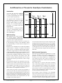
Figure 1. Interpreted noise and analysis overview
of the device) which the user wishes to access in order to
perform calculations. For example a model parameters file
for a JFET model contains parameters such as transconductance parameter gain, modulation coefficient, saturation current, and threshold voltage, required to define
the behavior of the analyses functions for the model.
SmartSpice translates the model parameters file into
template files (including one for noise analysis) which
contains data definitions and a function definition with
appropriate parameters into which the user defined code
for the noise analysis function is placed. This modified
file is interpreted by the SmartSpice C-Interpreter in
order to perform the noise analysis.1
1This file may also be compiled to object format which can be placed into a dynamic
link library for faster run time execution.
Continued on page 2....
INSIDE
Interpreted Noise Analysis Interface
An Efficient Use of Threads for SmartSpice Parallelization . . . . 3
The SmartSpice noise analysis interface extends those already present within SmartSpice and is shown in Figure 1.
Advanced SmartSpice Command Functionality . . . . . . . . . . . . . 5
The model parameters file in Figure 1. contains any
model and model instance parameters (parameters
which are used to encode the behavioral characteristics
Volume 8, Number 7, July 1997
Trouble-Shooting GPIB Communication Problems . . . . . . . . . . . 7
Generation of a New SPAYN Database
from a Limited Data Set . . . . . . . . . . . . . . . . . . . . . . . . . . . . . . 8
Calendar of Events . . . . . . . . . . . . . . . . . . . . . . . . . . . . . . . . . . . 9
Hints, Tips, and Solutions . . . . . . . . . . . . . . . . . . . . . . . . . . . . . . 10
Noise analysis is initiated via the .noise card from the
SmartSpice input deck. In order to use a user defined
noise analysis function to perform noise analysis for a
user defined model, the user needs to modify the .model card for the associated user defined model, modify
the element statement which instantiates the model and
direct SmartSpice to the user defined noise analysis
function within the interpreted C file.
Example of Syntax Required
The following example illustrates some excerpts from
SmartSpice statements which show how noise analysis
may be employed. Once the user has produced the
template file for noise analysis via SmartSpice translation of a model parameters file2, the .model is modified in order to direct SmartSpice to the location of the
noise function and file it is contained within. This is
shown below:
.MODEL JMOD NTYPE (
+ userparams = jfet_parameters
+ VTO = -2.50051
This performs a noise analysis of the circuit with 10
frequency points from 1 to 10 GigaHertz with V(1) the
output port referred to VGS.
Finally, shown below is a portion of an interpreted noise
analysis function to give a flavor of what is required.
/* instance parameters */
static int INSTicVDS
=
static int INSTicVGS
=
static int INSTarea
=
static int INSTwidth
=
static int MODELtype
=
static int MODELsourceResist =
static int MODELdrainResist =
tempsourcecode = jfettemp.int tempfunction = jfettemp
+
acsourcecode = jfetac.int acfunction = jfetac
+
noisesourcecode = jfetnoise.int noisefunction = jfetnoise
0;
1;
2;
/* type
/* rd
/* rs
*/
*/
*/
/* parameter list incomplete */
double
double
double
double
double
double
double
double
double
int
double
double
+ )
.END
freq;
NstartFreq;
lstFreq;
delFreq;
*outNoiz;
*inNoise;
lnFreq;
lnLastFreq;
delLnFreq;
*outNumber;
*outpVector;
*OnDens;
/*
/*
/*
/*
/*
/*
/*
/*
/*
/*
/*
/*
current frequency of noise analysis
start frequency of noise analysis
last frequency of noise analysis
last current frequency difference
total output noise
total input noise
natural log of current frequency
natural log of last frequency
natural log of last/current freq. diff
number of noise calculations
output vector of noise calculations
output noise density
)
The line noisesourcecode = jfetnoise.int
noisefunction = jfetnoise provides SmartSpice
with the noise function name jfetnoise and filename
jfetnoise.int
The model element definition indicates whether or not
the SmartSpice interactive debugger is activated during
execution of the interpreted code.
YJ1 3 2
1 2 0
{
/* calculate device terminal noise contributions */
/*
* assign noise calculations to appropriate ``reference’’
* parameters for SmartSpice to access
*/
/* return to SmartSpice */
}
JMOD
+ userparams = jfet_parameters
+ W=
1.00E-05 L=
The scope of this paper is not to describe the calculations
involved. The above serves only to show the outline of
the noise function given to the user and some of the
parameters which are accessed and used from within
the noise function. The instance and model parameters
at the top of the files are used to access arrays containing
their corresponding values. A fuller description of this
process is provided in [1].
1.00E-05
+ dcdebug = 0 tempdebug = 0 acdebug = 0 noisedebug = 1
The line + dcdebug = 0 tempdebug = 0 acdebug
= 0 noisedebug = 1 indicates that the interactive
debugger should be activated on interpreting the noise
analysis function but not the DC, temperature or AC
analyses functions.
The .noise card directs SmartSpice to perform a noise
analysis of the circuit.
References
[1]
SmartSpice User Manual Vol 2 Silvaco International, March 1997
.noise V(1) VGS DEC 10 1 10G
2Trivial process performed by SmartSpice buildtemplates command, refer to
[1].
TCAD Driven CAD
*/
*/
*/
*/
int jfetnoise(
double *instance;
/* access to array of instance parameters
*/
double*model;
/* access to array of model parameters */
int
*instanceGiven;
/* access to instance parameters flags
*/
int
*modelGiven;
/* access to model parameters flags
*/
int
iteration_number; /* solution iteration number
*/
char *device_name;
/* user defined device name
*/
+ CGS = 1.08825E-12 PB = 0.8 FC = 0.5
dcsourcecode = jfetdc.int dcfunction = jfetdc
icvds ic_vds
icvgs ic_vgs
area
w
/**********************************************************************/
/*
jfetNOISE */
/**********************************************************************/
+ RS = 3.004572 IS = 4.3694E-14 CGD = 1.086E-12
+
/*
/*
/*
/*
/* Model parameters */
+ BETA = 3.83708E-3 LAMBDA = 0.0664762 RD = 27.40726
+
0;
1;
2;
3;
Page 2
July 1997
*/
*/
*/
*/
*/
*/
*/
*/
*/
*/
*/
*/
An Efficient Use of Threads for SmartSpice Parallelization
Introduction
As circuit size and time simulation
increase dramatically any technique
to reduce computational time can be
crucial to improve productivity.
Our approach takes advantage of recent technology advances in bot h
hardware and software on multiprocessor SMP machines. It relies on
intensive use of multi-threaded programming via the IEEE POSIX 1003
implementation.
Main Thread
Active
Time
Thr 1
Idle
Thr 2
Active
Active
Idle
In the first part we briefly present the
concept of multi-threading, then we
will show how we have used it to parallelize SmartSpice.
Thr 3
Synchronization
Active
Multi-threading
Idle
With multiprocessors systems available
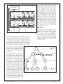
on several popular architectures, FIGURE 1. Master-slave paradigm running on 4 processors
multi-threaded programming provides
a powerful way to speed-up computationally intensive programs. This part describes how
A second useful control structure is the workpile. In this
to take advantage of some of the capabilities offered
paradigm the threads get their job from a set of chunks
by multi-threading in a shared memory multiprocessor
of works usually organized as a queue. The threads keep
environment.
taking new jobs from the queue until it is empty. The
second approach can be more flexible than the previous
Threads are a new and efficient way to utilize the parallelism
one, as it lets the threads compete with each other to get
of the hardware. A thread is a sequence of execution
their tasks.
within a process. A traditional single-threaded application follows a single sequence of control while executing.
Multi-threaded Smartspice
A multi-threaded process has several sequences of control, this allows several independent actions to occur at
The first step in parallelizing an application is to isolate
the same time. In addition, the threads can share a large
the time consuming tasks, as they will be the most
amount of data within the same address space. This
productive in terms of speed-up. In SmartSpice, an
provides extremely high bandwidth and low latency
execution cycle consists mainly in an assembly phase
communication between parallel tasks within a single
and a matrix inversion. This is shown by Figure 2. In
application.
this figure, the difference is made between parallel and
To speed-up the program, the computation must be divided into a set of tasks so that the tasks interact little
with each other and so that the number of tasks can be
easily adapted to the number of processors. There are
many ways to make a program parallel, thought the
main concern is to avoid processor starvation.
A first natural way follows a master-slave paradigm or
control structure. The main master thread launches a set
of slave threads with a predefined portion of the work to
be done. The master starts the threads and then waits for
all them to terminate at a synchronization point. In our
case this must be done every computational cycle. This
paradigm is illustrated in Figure 1.
TCAD Driven CAD
sequential execution.
The second step is to analyze these time consuming
tasks to find what paradigm will be more accurate in
order to parallelize them. In standard circuit simulation,
most of the time is spent in assembling and inverting a
sparse matrix, each row of which represents a node in
the circuit. The parallelization of these two phases will
be discussed in the following sections.
The load phase consists essentially in two embedded
loops. Every instance of every model in the circuit is successively evaluated and then stored in a sparse matrix
and a right hand side. The amount of work to be done
is known in advance and the computation can be easPage 3
The Simulation Standard
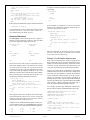
The ancestor-descendant relations contained
into structure of the elimination tree is now
used to build a queue of tasks. Each node
will be assigned to levels so that each level
contains completely independent columns
whose computation can be made in parallel.
The scheduling queue is constructed so that
the tasks in the queue have increasing level
numbers. Each thread will pick up the first
available task in the queue and compute the
corresponding column having previously
checked that all the tasks of the previous level
were completed, this ensures that all dependency constraints will be verified. This control
structure is very close to a workpile paradigm
and is the most suitable for very sparse SPICE
matrix elimination.
Time advance
Parallel load
Thr 1
Thr 2
Thr 3
Thr 1
Thr 2
Thr 3
Sync
Parallel LU
factorization
Sync
Conclusion
Solve
The parallelization of SmartSpice, has been
performs a very accurate manner in order
to preserve the accuracy of the simulator.
The accuracy of sequential SmartSpice, is
successfully maintained when the simulation
speed is noticeably increased. Some speed-ups
are presented in the May 1997 issue of The
Simulation Standard and new results will
soon be published.
Figure 2. A time step in Parallel SmartSpice on 4 processors
ily split in independent tasks. Load balancing is thus
obtained naturally by splitting the loops in chunks of
the same size. It is then very convenient and efficient
to use a master-slave paradigm to schedule the computation, between the threads. The master-slaves waits for all
slave threads to complete their work and then continues
the simulation. The assembly phase presents a typical
coarse level of parallelism. Note that
the performance can be improved by
letting the master thread do a part of
the job instead of waiting for the slaves
to join him.
7
level 3
10
5
In SPICE the matrix inversion is
performed using a Gaussian elimination with pivoting. Although this LU
decomposition with pivoting is a robust
algorithm to solve a symmetric sparse
linear systems, its efficient parallel implementation is not obvious. Before the
5
factorization, a re-ordering of the matrix
for sparsity and accuracy may occur.
Then as a first step in parallel factorization, the elimination tree is built. The
elimination tree is the smallest structure
that shows dependency informations be1
tween the elimination of the unknowns
of the system. Each node of the tree will
represent a column of the matrix. A col- Figure 3. Elimination tree.
umn corresponding to a node must be
computed after all its children nodes
in the tree. In the example below, node
3 must be computed after nodes 6 and 9.
8
1
8
TCAD Driven CAD
6
Page 4
4
3
2
level 2
9
2
6
9
3
10
7
level 1
level 0
4
July 1997
Advanced SmartSpice Command Functionality
Unlike most commercial simulators, SmartSpice, provides the user with a powerful command interface. This
command interface is used extensively in SmartSpice,
to implement the Graphical User Interface. Every action
the user performs via menus and dialogs is translated
into an equivalent command which is then executed by
SmartSpice.
mand is used to create a variable and set it to the required value. The value can be numeric, string, boolean
or a list.
% set
% set foo = 1.5
% set rtscreen
% set alist = ( a b c d e f g h i j k l m n o )
For example, when the “Source” dialog is used to load
and parse an input deck, the source command will be
generated and executed. This command will then appear in the output area. If the user simulates the
circuit and then plots some output waveforms, then the
corresponding run and plot commands are used.
The set command with no arguments will display the
current list of defined variables. The second command
will create the variable “foo” and set it equal to 1.5. The
variable “rtscreen” is a SmartSpice system variable and it
is set to true in the third command. The last command creates the variable “files” and sets it equal to a list of strings.
Commands are not only used in the GUI, but are also
used when the simulator is run in batch mode, (using
the -b command-line option). In this case, the commands
to source the input deck(s), simulate and perform
post-processing are automatically and transparently
executed by SmartSpice.
The value of a variable can be accessed by the standard
$var notation. To access an element of a list, use the
$var[low-high] notation. If a variable contains a list, then
the number of elements in the list can be accessed using
the notation $#var. The special variable $$ contains the
PID of the executing SmartSpice process.
In addition, many SmartSpice input deck statements
have corresponding commands. When such a statement
is executed, it is translated into the equivalent command and this is executed. For example, SmartSpice
supports the .MEASURE statement and measure command.
The .MEASURE statement is executed as a post-processing
step when a simulation is completed. The measure command can be used at any time and will be applied to the
current plot. This plot can be the result of a completed
simulation or could have been loaded from a previously
loaded rawfile. Some examples of statements with equivalent commands are;
Statement
.OP
.DC
.AC
.TRAN
.MEASURE
.PLOT
.PRINT
% echo “There are” $#alist “elements is alist”
There are
Elements 5-7 (
e f g
)
When the measure command is used, a variable is created
to store the results of the measurement. This value can
then be used in subsequent commands.
% measure max_vout max abs(v(out))
% echo “The maximum voltage at node \”out\” is” $max_vout
Command
op
dc
ac
tran
measure
plot
print
Command Scripts
A command script is a collection of commands in a file
that SmartSpice will execute. These commands appear
within a .CONTROL .... .ENDC block in an input deck. If
a netlist also exists in the deck, then SmartSpice will first
parse the deck, before executing the commands in the control block. SmartSpice will only parse the netlist and will
not execute any analysis statements. To run the simulation,
the run command must be used within the control block.
An input deck need only contain a control block, and this
case resembles a standard shell script approach.
C-Shell Like Commands
The functionality of the SmartSpice command set has
been extended by the addition of csh like features.
These features include creation of aliases, filename
completion, global, variable and history substitution,
I/O redirection and control structures. Some of these
features, e.g. filename completion are only available
when SmartSpice is run is command mode, (using the
-c command-line option).
Note: A command script is parsed in the same manner
as any other SmartSpice input deck, hence, the
first line of the deck is used as a TITLE line and will
be ignored. It must not be used to start the control
block.
Variable Usage
Comments can be embedded within the control block
using the # character. This character can appear anywhere
on a line and everything after it will be discarded.
Variables can be used by the command interpreter to
store and manipulate strings or numbers. The set com-
TCAD Driven CAD
15 elements is alist
% echo “Elements 5-7 ( “ $alist[5-7] “ )”
Page 5
The Simulation Standard
To support conditional operation, the following structure
is provided,
* Title line (will be ignored)
.CONTROL
source test.in
run
measure rtime delay v(out) rise=1 val=0.5 targ \
v(out) rise=1 val=4.5
measure ftime delay v(out) fall=1 val=4.5 targ \
v(out) fall=1 val=0.5
echo “Rise Time =” $rtime > test.res
echo “Fall Time =” $ftime >> test.res
if condition
command
else
command
end
.ENDC
If this script is stored in the file “script.in”, then the command
If the condition is evaluated to a non-zero value, then
the first set of commands is executed, otherwise the second set of commands is executed.
% smartspice -b script.in
will load the deck “test.in”, simulate, measure the output
rise and fall times, and store these results in a
user-defined format in the file “test.res”.
foreach plot tran{1,2,3,4,5,6}
setplot $plot
measure max_out max v(out)
Command Structures
if $max_out lt 2.5
The SmartSpice command interpreter also supports a
number of control structures similar to those provided
by csh. The supported looping structures are
foreach var value
command
.
.
.
end
repeat number
command
.
.
.
end
while condition
command
.
.
.
end
dowhile condition
command
.
.
.
end
echo $plot “failed (“$max_out”)” >> test.res
else
echo $plot “okay (“$max_out”)” >> test.res
end
end
The break command can be used to exit from a looping
structure, and the continue command can be used to
move to the next value of the loop.
Example: Post Simulation Measurement
In the case of long simulations, which can generate very
large rawfiles, the “rawpts” options is often used to incremently write data to disk. This helps reduce the amount
of memory used by the simulator and allows the user to
view partial results before the simulation has finished.
The foreach structure will execute its commands once for
each of the supplied values, and each time the variable
var will be set to the current one. repeat will execute the
commands number times. The while and dowhile structures
will execute until the supplied condition is false. The
difference is that the while command will test the condition
before executing the commands, but the dowhile command will test after the commands are executed.
However, use of this option will disable use of the .MEASURE statement, since at any one time only a small portion
of the data will be available. To perform measurements
on the output data, while allowing use of the “rawpts”
option, it is necessary to use the measure command. To
automate this procedure, copy the .MEASURE statements
from the input deck into a script file. Replace .MEASURE
with “measure”, convert everything to lowercase and remove any analysis identifier from the command.
foreach plot 1 2 3 4
setplot tran{$plot}
echo “Transient Analysis, #”$plot >> test.res
foreach vector v(out1) v(out2) v(out3)
measure del delay v(in) val=2.5 targ $vector
val=2.5
echo “ Rise Time :” $vector “=” $del >>
test.res
end
end
For example, the following .MEASURE statements in
the input deck would be replacedthe following script.
.MEASURE TRAN delay1 DELAY v(in) rise=1 val=2.5
+TARG v(out1) rise=1 val=2.5
.MEASURE TRAN delay2 DELAY v(in) rise=1 val=2.5
+TARG v(out2) fall=1 val=2.5
This example will measure the delay between the input,
v(in) and each of the output vectors, v(out1), v(out2) and
v(out3), for each of the plots tran1, tran2, tran3, tran4. It
will then store these results in “test.res”.
* Measure Script 1
Conditions can use standard relational operators as in C, however it is normally safer to use the FORTRAN-like synonyms
as the ‘<’ and ‘>’ can be confused with redirection operators.
<
>
=
lt
gt
eq
<= le
>= ge
<> ne
TCAD Driven CAD
&
|
!
and
or
not
.CONTROL
load test.raw # Load the generated rawfile.
measure delay1 delay v(in) rise=1 val=2.5
targ
\
v(out1) rise=1 val=2.5
measure delay2 delay v(in)
targ
\
rise=1
val=2.5
v(out2) fall=1 val=2.5
.ENDC
Page 6
July 1997
Trouble-Shooting GPIB Communication Problems
Communicating via the HP-IB interface
Instrument communication in UTMOST is performed
in one of two ways: either through the serial port,
connected to an external serial-to-GPIB interface or,
on certain HP workstations, through an internal HP-IB
interface. The purpose of this note is to describe the
most frequently occuring problems with both of these
interfaces, along with how to cure them.
Direct GPIB communication is provided on some HP
9000 Series 700 workstations in the form of the optional, internal HP E2070 HP-IB Interface or HP E2071
High Speed HP-IB Interface; on the 745i, 747i or V743
workstations the Built-in HP-IB Port serves the same
purpose. The “CPU side” button in the UTMOST Device
Configuration screen should be set to either “GPIB Port
1” or “GPIB Port 2” in this case, and the “GPIB symbolic
name” in the GPIB Port Setup screen is typically set to
“hpib”, although this name may be changed in the manner described below.
Communicating Via the Serial Port
Serial port commuincation is carried out through the
National Instruments GPIB-232CT or GPIB-232CT-A serial-to-GPIB interface, whose configuration is described
in detail in Appendix B of the UTMOST User’s Manual.
The “CPU side” button in the UTMOST Device Configuration screen should be set to either “Serial Port 1”
or Serial Port 2”, and the “Port Name” field in the Serial Port Setup screen should be set to the appropriate
name, ie. “ttya” or “ttyb” for Sun, “tty00” or “tty01” for
HPUX 9 and Dec Alpha, “tty0p0” or “tty1p0” for HPUX
10, “tty0” or “tty1” for IBM and “ttyd1” or “ttyd2” for
SGI (these, and other setup options are described in Appendix B). These values map directly to the UNIX files
/dev/ttya, /dev/tty00, etc., depending on the machine
in use.
If polling does not succeed with this configuration, then
the first thing to check is whether or not the necessary
HP SICL (Standard Instrument Control Library) has
been installed. This will result in the existence of the
directory /usr/pil on HPUX 9 machines, and of the directory /opt/sicl on HPUX 10 machines. If one or the
other of these directories does not exist, then the missing
libaries can be obtained from the HP E2091D software
update, entitled “HP I/O Libraries for Instrument Control”. This software should be installed using either the
/etc/update command on HPUX 9, or the /usr/sbin/
swinstall command on HPUX 10. The filesets which
are required are: PIL-HPIB and PIL-RUN on HPUX 9,
and SICL-HPIB and SICL-RUN on HPUX 10. The user
should be aware that this procedure will rebuild the
UNIX kernel and reboot the system.
An inability to poll selected instruments is frequently due
to a mismatch between the configuration in the Serial Port
Setup window and the switch settings on the GPIB-232CT,
a failure in the GPIB-232CT itself, or a simple break in the
serial cable connecting the GPIB-232CT to the workstation.
If these failures have been eliminated and polling is still
not successful, then it is quite likely that insufficient
permissions have been set on the device files. To verify
whether or not this is the case, the underlying device file
must be located for the serial port in question. This may
not be the file in the /dev directory, as some machines
use symbolic links to locate their device files elsewhere
(for instance, on Solaris 2 machines, the file /dev/ttya is
actually a symbolic link to /dev/term/a, which is itself
a link to an obscurely named file beneath the /devices
directory). The command:
Associated with each HP-IB Interface is a logical unit
number and a symbolic name. These may be quickly
determined by examing the last few lines of the file
/usr/pil/etc/hwconfig.cf, on HPUX 9, or /opt/sicl/etc/
hwconfig.cf, on HPUX 10. A typical such file might end
with:
# E2071 High Speed HP-IB
7 hpib e2071 1 21 0b0000 1 3
which describes a single interface with logical unit
number 7 and symbolic name “hpib”. These values can
be altered with the command /usr/pil/bin/iosetup on
HPUX 9, or /opt/sicl/bin/iosetup on HPUX 10, run as
superuser. In any event, this command must be executed
after the initial installation of the SICL filesets, in order
to create the necessary instances of HP-IB or High Speed
HP-IB Interface setups.
ls -l <device file>
can be used to follow symbolic links as necessary, where
<device file> takes the value of the current file under
investigation. Once the underlying device file has been
located in this manner, a sufficient set of permissions
can be set, by the superuser, with the command:
One further step is also necessary after the initial
installation: either the HP-IB Interface Device Driver or
the High Speed HP-IB Device Driver must be added to
the UNIX kernel. This is easily done with the system
administration tool /usr/bin/sam on HPUX 9, or /usr/
sbin/sam on HPUX 10, under the “Kernel Configuration->Drivers” area. This action will also cause the
system to reboot.
chmod a+rw <device file>
If polling is still unsuccessful at this point, then it may be
necessary to reconfigure the serial port drivers, although
in practice this is fairly uncommon. The mechanics of
this process vary between machines and operating systems, so the appropriate manual pages should be consulted for detailed operating instructions.
TCAD Driven CAD
Page 7
The Simulation Standard
Generation of a New SPAYN Database
from a Limited Data Set
SPAYN is a very comprehensive statistical tool designed
specifically for semiconductor industry. One of the main
features of SPAYN is the ability to perform analysis on
the measured data collected from wafers. This generates
information on dominant parameters and can be used
for physically based worst case analysis.
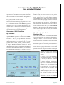
specify the joint distribution of those parameters you
need to specify the mean and sigma for each parameter, and then possibly may specify the correlation
matrix. In this example we consider all five parameters
are independent of each other. Click on the Generation
Window..., there should pop up a Database Generation
window. Enter the Number of Simulation points on the
first text field and click on Generate... button at the bottom of the window. We could also choose one of the two
formats for the simulation data, one is standard SPAYN
Database the other is Comma Separated Values. Give a
filename on the popup Destination Filename window
and hit return or press the store button, the simulated
data is then generated and stored in this file.
However, sometimes collecting a large data base is not
feasible for some applications. In this case it is possible
to use the built-in simulator inside SPAYN to generate
data based on our past experience about the model parameters. This can be useful for those characterization
engineers who are developing a new technology or are
not able to access a large measured database.
Generation of SPAYN Data Base
By Simulation
Worst Case Analysis On the
Simulation Data
First start VYPER in your working directory and then
open the SPAYN application window inside VYPER.
On the main SPAYN window go to File->Operations->DB
From Stats.... This will pop up a Database Generation
Setup Window. In this example we are going to generate a
database including five parameters. We give them
general names as Param_1, Param_2, Param_3, Param_
4, Param_5. But these parameters could be any SPICE
model parameters we think that are important and whose
distribution is known based on experience. In the Database
Generation Setup Window (see Figure 1.) we would first
input the number of parameters to consider. In order to
Use the File->Load/Import... to load the simulation data
we just generated. Now we could first use the Analysis>Histogram feature to see how good our simulation
data is. Since the simulation is to generate multidimensional Gaussian distribution, we would see that
each parameter is fit by a one dimensional Gaussian
distribution quite well. Now if the parameter data are
correlated, i.e. the correlation matrix is not the identity
matrix when we are doing the simulation, we may need
to use the Groups/Equations->PCA/PFA feature to
perform a Principal Component Analysis or Principal
Factor Analysis to find independent
dominant parameters and reduce the
number of parameters for worst case
analysis.
In our case, we start with five independent dominant parameters, so we could
go directly to define our dominant
parameters using four parameters out
of the five parameters. Use Groups/
Equations->User-defined->Dominant
Parameters... feature to accomplish this
definition. Now the Simulation Menu
bar becomes active, so we could go to
Simulation->All User Dominant..., this
would give us a Simulation Interface
window(see Figure 2.). Now use one of
many methods available in this simulation window to generate corner models, and save them as a .lib file for circuit
simulation. Or we could use VYPER to
Figure 1. Database Generation Setup Window.
Continued on page 11....
TCAD Driven CAD
Page 8
July 1997
Calendar of Events
July
1
2
3
4
5
6
7
8
9
Workshop - Guildford
Workshop - Munich
Workshop - Japan
Workshop - Grenoble
10 Workshop - Japan
11 Workshop - Japan
12
13
14
15
16
17
18
19
20
21
22
23
24
25
26
27
28
28
30
31
August
1
2
3
4
5
6
7
8
9
10
11
12
13
14
15
16
17
18
19
20
21
22
23
24
25
26
27
28
29
30
31
Bulletin Board
Silvaco To Demonstrate Advanced
Model Implementations at BCTM ‘97
Silvaco will be demonstrating the new models and
features that have been incorporated into SmartSpice,
the rapidly emerging industry standard for analog
circuit simulation, and UTMOST the established industry
standard for parameter extraction and SPICE modeling.
Silvaco’s engineers will be demonstrating the advanced
BSIM3v3.1 sub-micron MOS implementations and
enhanced capabilities of SmartSpice and UTMOST for
Bipolar technologies. New supported Bipolar models
include the Mextram v5.03.2 and VBIC95 v1.1.5 models.
The IEEE Bipolar / BiCMOS Circuits and Technology
meeting will be held on September 29th - 30th at the
Minneapolis Marriott City Center.
ChiPPs ‘97, Germany
ChiPPs ‘97, Germany
ChiPPs ‘97, Germany
TCAD W/S, Japan
New Instrument Drivers in UTMOST III!
To enhance the noise measurement capability of
UTMOST III, a set of new device drivers is developed:
HP35660 Dynamic Signal Analyzer
HP35665 Dynamic Signal Analyzer
HP35670 Dynamic Signal Analyzer
The following Le Croy Oscilloscope driver is
implemented in UTMOST III to enhance ring oscillator
measurements:
9374 Le Croy Oscilloscope
EUROPAR, Germany
Characterization Lab Expands!
To accommodate a rising demand for SPICE Modeling
Service, Silvaco has significantly expanded the lab
capability. A set of new instruments is added: HP4155,
HP8753D, HP3561. Silvaco now offers on wafer
s-parameter measurements, ring oscillator and noise
measurements as modeling services.
For more information on any of our workshops, please check our web site at http://www.silvaco.com
The TCAD Driven CAD, circulation 15,000, Vol. 8, No. 7, July 1997 is copyrighted by Silvaco International. If you, or someone you know wants a subscription to this
free publication, please call (408) 567-1000 (USA), (44) (1483) 401-800 (UK), (81)(45) 820-3000(Japan), or your nearest Silvaco distributor.
Simulation Standard, TCAD Driven CAD, Virtual Wafer Fab, Analog Alliance, Legacy, ATHENA, ATLAS, FAST ATLAS, ODIN, VYPER, TSUNAMI, RESILIENCE,
TEMPEST, CELEBRITY, Manufacturing Tools, Automation Tools, Interactive Tools, TonyPlot, DeckBuild, DevEdit, Interpreter, ATHENA Interpreter, ATLAS
Interpreter, Circuit Optimizer, MaskViews, PSTATS, SSuprem3, SSuprem4, Elite, Optolith, Flash, Silicides, SPDB, CMP, MC Deposit, MC Implant, Process
Adaptive Meshing, S-Pisces, Blaze, Device 3D, Thermal 3D, Interconnect 3D, TFT, Luminous, Giga, MixedMode, ESD, Laser, FastBlaze, FastMixedMode, FastGiga,
FastNoise, UTMOST, UTMOST II, UTMOST III, UTMOST IV, PROMOST, SPAYN, SmartSpice, MixSim, Twister, FastSpice, SmartLib, SDDL, EXACT, CLEVER,
STELLAR, HIPEX, Scholar, SIREN, ESCORT, STARLET, Expert, Savage, Scout, Guardian and Envoy are trademarks of Silvaco International.
TCAD Driven CAD
Page 9
The Simulation Standard
Hints, Tips and Solutions
Mustafa Taner, Applications and Support Engineer
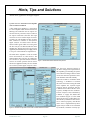
Q. How can I use the S3245 Noise amplifier
with or without UTMOST?
A The S3245 Noise amplifier is a stand alone
low noise amplifier which includes the DC bias
filterings. The S3245 has four DC inputs connected to the DC parameter analyzer and four
DC outputs connected to the DUT. The input
connectors are triax and the output connectors
are BNC type. The amplifier also has one more
BNC connector to interface to the Dynamic
Signal Analyzer for Flicker Noise measurements. The DC signals which are coming from
the DC analyzer are filtered inside the Noise
amplifier box. The DC bias for the op-amps are
supplied by the shielded DC power supply which
is also part of the S3245 Noise amplifier box.
The S3245 Noise amplifier is used for Flicker
Noise measurements on MOS devices. The
S3245 amplifier does not have any GPIB interface and can be operated without UTMOST’s Figure 1. Noise Measurement Routine Setup Screen.
control. In manual operation the DC biases
should be supplied manually. The user should
also set the Dynamic Signal Analyzer to measure the Power Spectrum Density of
the Noise Voltage and compensation of
the amplifier gain including the system
noise. The Noise Voltage to Noise Current
conversions and Noise parameter extractions should be cariied out manually.
Figure 2. Hardware configuration screen with new DSA instrument drivers.
TCAD Driven CAD
Page 10
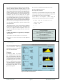
The Noise module in UTMOST’s MOS
technology is modified to automate
the Noise measurement using the S3245
Noise amplifier box, Dynamic Signal
Analyzer and DC parameter analyzer.
UTMOST Noise routine will allow users
to specify multiple DC bias conditions.
The DC analyzer will be controlled by
UTMOST to supply the defined DC
bias conditions (Figure 1.) to the S3245
input. The necessary settling delays are
introduced by UTMOST for DC line filters to function properly. After the the
device noise is amplified the Dynamic
signal analyzer which is also controlled
by UTMOST ( UTMOST currently sup-
July 1997
ports the following Dynamic signal Analyzers HP3561,
HP3562, HP35660, HP35665, HP35670 (Figure 2.)) will
start the measurement of Power Spectrum Density of the
Noise Voltage. The measured noise will be displayed on
UTMOST graphics screen and the same measurement
process will be repeated for the other specified DC bias
conditions. The user can also utilize the “fit” option
from the graphics screen to extract the Noise paramaters (including BSIM3 Noise parameters). The extracted
SPICE parameters can be verified by using UTMOST’s
SPICE simulator interface and measured and simulated
noise curves can be overlayed. The user can also exercise the “Global Optimization” option to improve the
noise parameters.
●
University of Southampton, STAG SOI model,
●
Berkeley BSIM3 SOI model,
●
Honeywell SOI model.
SOI devices are instantiated in the input deck as MOS
devices and the respective level numbers for the models
in SmartSpice are Level 21, 22, 24, 23 and 20.
Shown below is an example of a device using the
STAG model. This particular device has 6 terminals.
M1 d fg s bg sub th nmod l=1u w=1u
.MODEL nmod NMOS (
+ Level = 24
The measured Noise curves can be stored in UTMOST
log file format and measured versus simulated noise
curves can be plotted. When multiple DC biases are
used the VDS and VGS voltage versus KF curves can
be obtained.
+ ......
+ )
Call for Questions
If you have hints, tips, solutions or questions to contribute, please
contact our Applications and Support Department
Phone: (408) 567-1000
Fax: (408) 496-6080
e-mail: [email protected]
Q: What SOI models are supported by SmartSpice
and UTMOST?
A: SmartSpice currently supports five SOI models:
●
Hints, Tips and Solutions Archive
University of Florida, non-fully and fully depleted
models,
Check our our Web Page to see more details of this example plus an
archive of previous Hints, Tips, and Solutions
http:://www.silvaco.com
....continued from page 8
call a circuit simulator directly for
worst case simulation. At this stage
the operations are pretty much the
same with measured data.
Summary
In summary, when we do not
have enough measured data, but
have some knowledge of how the
important parameters are distributed,
we could use the built-in simulator
in SPAYN to generate data according to our distribution knowledge
of model parameters and perform
worst case analysis on this simulation database and generate circuit
performance spread.
Figure 2. Simulation Interface Window.
TCAD Driven CAD
Page 11
The Simulation Standard
SILVACO WANTS YOU!!
The last significant independent TCAD and SPICE
developer invites you to join our team . Find out
what our engineers are so excited about!
●TCAD Developers
● TCAD Application Engineers
● Software Developers
● SPICE Application Engineers
fax your resume to:
408-496-6080, or
e-mail to:
[email protected]
4701 Patrick Henry Drive, Building 2
Santa Clara, CA 95054
Telephone:
Fax:
URL:
(408) 567-1000
(408) 496-6080
http://www.silvaco.com
Opportunities worldwide for apps engineers: Santa Clara, Phoenix, Austin, Boston,
Tokyo, Guildford, Munich, Grenoble, Seoul, Hsinchu. Opportunities for developers
at our California headquarters.