1
XSHELLS 1.1 : User Manual
Nathanaël Schaeffer
ISTerre/CNRS
July 15, 2015
Chapter 1
Getting Started
1.1
Description
XSHELLS is yet another code simulating incompressible fluids in a spherical cavity. In
addition to the Navier-Stokes equation with an optional Coriolis force, it can also timestep the coupled induction equation for MHD (with imposed magnetic field or in a dynamo
regime), as well as the temperature (or codensity) equation in the Boussineq framework.
XSHELLS uses finite differences (second order) in the radial direction and spherical
harmonic decomposition (pseudo-spectral). The time-stepping uses semi-implicit CrankNicolson scheme for the diffusive terms, while the non-linear terms can be handled either
by an Adams-Bashforth or a Predictor-Corrector scheme (both second order in time).
XSHELLS is written in C++ and designed for speed. It uses the blazingly fast spherical
harmonic transform library SHTns, as well as hybrid parallelization using OpenMP and/or
MPI. This allows it to run efficiently on your laptop or on parallel supercomputers. A postprocessing program is provided to extract useful data and export fields to matlab/octave,
python/matplotlib or paraview.
XSHELLS is free software, distributed under the CeCILL Licence (compatible with
GNU GPL): everybody is free to use, modify and contribute to the code.
1.2
Requirements
The following items are required :
• a Unix like system (like linux),
• a C++ compiler,
• the FFTW library, or the intel MKL library.
• the SHTns library,
The following items are recommended, but not mandatory:
1
• a C++ compiler with OpenMP support,
• an MPI library (with thread support),
• the HDF5 library for post-processing and interfacing with paraview,
• Python 3, with NumPy and matplotlib (Python 2.7 should also work),
• a processor supporting the AVX instruction set.
• Gnuplot, for real-time plotting.
1.3
Installation
FFTW and SHTns must be installed first. FFTW comes already installed on many systems,
but in order to get high performance, you should install it yourself, and use the optimization
options that correspond to your machine (e.g. --enable-avx). Please refer to the FFTW
installation guide.
Note that it is possbile to use the intel MKL library instead of FFTW. To do so, you
must configure both SHTns and XSHELLS with the --enable-mkl option.
To install SHTns, get the latest version of SHTns, extract it and run:
./configure
make
make install
This will install the serial version (without OpenMP) of SHTns, which is the one required
for XSHELLS. If you do not have administrator privileges, you can use ./configure
--prefix=$HOME to install it in your home directory. To choose another compiler than the
default one, use ./configure CC=my-c-compiler.
To install XSHELLS, grab the XSHELLS archive, extract it, and then run
./configure
to automatically configure XSHELLS for your machine. If you have used the --prefix
option when installing SHTns, you should pass the same one to configure for XSHELLS.
Type ./configure --help to see available options, among which --disable-openmp and
--disable-mpi.
Before compiling, you need to setup the xshells.hpp configuration file (see next section).
2
1.4
Configuration files
There are two configuration files:
• xshells.hpp is read by the compiler (compile-time options), and modifying it requires to recompile the program. The corresponding options are detailed in section
2.2.
• xshells.par is read by the program at startup (runtime options) and modifying it
does not require to recompile the program. This file is detailed in section 2.1.
See chapter 2 for more details. Example configuration files can be found in the problems
directory.
Before compiling, copy the configurations files that correspond most closely to your
problem. For example, the geodynamo benchmark:
cp problems/geodynamo/xshells.par .
cp problems/geodynamo/xshells.hpp .
and then edit them to adjust the parameters (see sections 2.2 and 2.1).
1.5
Compiling and Running
When you have properly set the xshells.hpp and xshells.par files, you can compile and
run in different flavours:
Parallel execution using OpenMP with as many threads as processors:
make xsbig
./xsbig
Parallel execution using OpenMP with (e.g.) 4 threads:
make xsbig
OMP_NUM_THREADS=4 ./xsbig
Parallel execution using MPI with (e.g.) 4 processes:
make xsbig_mpi
mpirun -n 4 ./xsbig_mpi
Parallel execution using OpenMP and MPI simultaneously (hybrid parallelization), with
(e.g.) 2 processes and 4 threads per process:
make xsbig_hyb
OMP_NUM_THREADS=4 mpirun -n 2 ./xsbig_hyb
3
1.6
Outputs
All output files are suffixed by the job name as file extension, denoted job in the following.
The various output files are:
• xshells.par.job : a copy of the input parameter file xshells.par, for future reference.
• xshells.hpp.job : a stripped-out version of the file xshells.hpp that was used
during compilation, for future reference.
• energy.job : a record of energies and other custom diagnostics. Each line of this
text file is an iteration.
• fieldX0.job : the imposed (constant) field X, if any.
• fieldX ####.job : the field X at iteration number ####, if parameter movie was set
to a non-zero value in xshells.par.
• fieldXavg ####.job : the field X averaged between previous iteration and iteration
number ####, if parameter movie was set to 2 in xshells.par.
• fieldX.job : the last full backup of field X, or field X at the end of the simulation.
Used when restarting a job.
All field files are binary format files storing the spherical harmonic coefficients of the field.
To produce plots and visualizations, they can be post-processed using the xspp program
(see chapter 3).
1.7
Limitations and advice for parallel execution
The parallelization of XSHELLS is done using a domain decomposition in the radial direction only (MPI and OpenMP). As a consequence, it is more efficient to use a number
of radial shells that is a multiple of the number of computing cores.
In addition, the number of MPI processes cannot exceed the total number of
radial shells. It is often more efficient to use a small number of MPI processes per node
(1 to 4) and use OpenMP to have a total number of threads equal to the number of cores.
Currently, using more threads than radial shells will speed up your calculation.
Because there is no automatic load balancing, some situations where the same amount
of work is not required for each radial shell will result in suboptimal scaling when the
number of MPI processes is increased. Such situations include (i) solid conducting shells
(e.g. a conducting inner core) and (ii) variable spherical harmonic degree truncation (e.g. in
a full-sphere problem). In these cases, especially the latter, use pure OpenMP or minimize
the number of MPI processes.
Using MPI executables (including hybrid MPI+OpenMP) is thus recommended only if
the following conditions are both met:
4
seconds per iteration
102
Performance scaling of xshells (NR=1024, Lmax=893)
Curie (SandyBridge)
101
102
number of cores
103
Figure 1.1: Performance scaling of XSHELLS on supercomputer Curie (thin nodes, SandyBridge processors) at TGCC (France). The ideal scaling is represented by the dashed black
lines. A geodynamo simulation was run with 1024 radial grid points and spherical harmonics truncated after degree 893.
• all fields span the same radial domain;
• the radial domain does not include the center r = 0 (and XS VAR LTR is not used, see
section 2.2.5).
In such cases, XSHELLS should scale very well up to the limit of 1 thread per radial shell
(see scaling example in Figure 1.1).
1.8
Citing
If you use XSHELLS for research work, you may cite the SHTns paper (because the high
performance of XSHELLS is mostly due to the blazingly fast spherical harmonic transform
provided by SHTns):
N. Schaeffer, Efficient Spherical Harmonic Transforms aimed at pseudo-spectral numerical simulations, Geochem. Geophys. Geosyst. 14, 751-758, doi:10.1002/ggge.20071
(2013)
5
Chapter 2
Setting up the simulation
Example configuration files can be found in the problems directory.
2.1
Run-time options: xshells.par
The file xshells.par is a simple text file. Each line may contain a single statement like
var = expression, or a comment starting with #. A simple math parser allows to use
convenient expressions like sqrt(4*pi/3).
All the following features can be set in xshells.par. There is no need to recompile if
this file is changed, as it is read and interpreted at program startup.
2.1.1
Equations and controlling parameters
XSHELLS can time-step the Navier-Stokes equation in a rotating reference frame. Optionally it can include (i) a buoyancy force in the Boussinesq approximation, where the
buoyancy obeys an advection-diffusion equation; and (ii) a Lorentz (or Laplace) force for
conducting fluids where the magnetic field obeys the induction equation. Precisely, the
following equations can be time-stepped by XSHELLS:
∂t u + (2Ω0 + ∇ × u) × u = −∇p∗ + ν∆u + (∇ × b) × b + c∇Φ0
∂t b = ∇ × (u × b) + η∆b
∂t c + u.∇(c + C0 ) = κ∆c
∇u = 0
∇b = 0
where
• u is the velocity field.
• c is a codensity (or temperature, or buoyancy) in the Boussinesq formulation.
6
(2.1)
(2.2)
(2.3)
(2.4)
(2.5)
•
√
µ0 ρ b is the magnetic field (ρ and µ0 are the fluid density and magnetic permeability,
but are not relevant for this equation set).
• ν is the kinematic viscosity of the fluid and is set by the variable nu in xshells.par.
• η = (µ0 σ)−1 is the magnetic diffusivity of the fluid (σ is its conductivity) and is set
by the variable eta in xshells.par.
• κ is the thermal diffusivity of the fluid and is set by the variable kappa in xshells.par.
• Ω0 is the rotation vector of the reference frame, which is usually along the vertical
axis ez . It is set by the variable Omega0 in xshells.par, while the angle (in radians)
between ez and Ω0 is set by Omega0 angle (0 by default). Note that Ω0 is always in
the x − z plane (φ = 0).
• Φ0 is the gravity potential (independent of time), controlled by field phi0 in xshells.par.
• C0 is the imposed base concentration (or temperature) profile, controlled by field tp0
in xshells.par.
• p∗ is the dynamic pressure deviation (from hydrostatic equilibrium), which is eliminated by taking the curl of equation 2.1.
Equation 2.1 (respectively 2.2 and 2.3) is time-stepped when u (respectively b and tp)
is set to an initial condition in xshells.par. Disabling an equation is as easy as removing
or commenting out the corresponding initial condition in xshells.par.
Example If the following lines are found in xshells.par:
nu = 1.0
eta = sqrt(10)
Omega0 = 2*pi*1e3
u = 0
b = 0
#tp = 0
then √
the viscosity is set to ν = 1.0, the magnetic diffusivity is set to
η = 10, and the rotation rate is set to Ω0 = 2π × 103 . The NavierStokes (2.1) and the induction equation (2.2) will be time-stepped, but
not the concentration (or temperature) equation (2.3), simulating an
isothermal fluid.
Note that it is up to the user to choose dimensional or non-dimensional control parameters.
7
Internal representation of vector fields
Vector fields are represented internally using a poloidal/toroidal decomposition:
u = ∇ × (T r) + ∇ × ∇ × (P r)
(2.6)
where r is the radial position vector, and T and P are the toroidal and poloidal scalars
respectively. This decomposition ensures that the vector field u is divergence-free.
The scalar fields T and P for each radial shell are then decomposed on the basis of
spherical harmonics.
2.1.2
Boundary conditions
Magnetic field boundary conditions are that of an electrical insulator outside the computation domain, with or without external sources of magnetic field (see section 2.1.3 for
externally imposed magnetic fields).
Temperature or buoyancy boundary conditions are either fixed temperature (defined
by the C0 profile) or fixed flux (defined by ∂r C0 ).
Velocity boundary conditions can be zero, no-slip (with arbitrary prescribed velocity at
the boundary) or stress-free.
The inner and outer boundary conditions can be chosen independently. The BC U (for
velocity) and BC T (for temperature/concentration) entries in xshells.par allow to select
the appropriate boundary conditions.
Example
The following lines in xshells.par define zero velocity and fixed temperature boundary condition at the inner boundary, and no-slip and fixed
flux boundary condition at the outer boudnary.
BC_U = 0,1
BC_T = 1,2
2.1.3
# inner,outer boundary conditions
# (0=zero velocity, 1=no-slip, 2=free-slip)
# 1=fixed temperature, 2=fixed flux.
Initial conditions and imposed fields
Predefined fields
Several predefined fields are defined in xshells init.cpp. The command ./list fields
prints a list of these predefined fields, with their name in the first column. You can simply
8
use this name in the xshells.par file to define an initial condition. You can also add your
own by editing xshells init.cpp.
Imposed fields are only supported for the gravity potential phi0 and for the basic state
of temperature/concentration tp0. Imposed magnetic fields can be obtained through the
appropriate boundary conditions (magnetic fields generated by currents outside the computation domain only). Some predefined magnetic field include these boundary conditions,
making them actually imposed fields (and are labeled as such).
Example The following lines in xshells.par set up the geodyanmo
benchmark initial conditions.
E = 1e-3
Pm = 5
Ra = 100
u = 0
# initial velocity field
b = bench2001*5/sqrt(Pm*E) # initial magnetic field (scaled by
#
sqrt(1/(Pm*E)))
tp = bench2001*0.1
# initial temperature field
tp0 = delta*-1
# imposed (base) temperature field
phi0 = radial*Ra/E
# radial gravity field (multiplied by
# Ra/E to match geodynamo benchmark)
Field files as initial conditions
In addition, any field file can be given as initial condition. If the radial grid is not the
same, the field must be interpolated on the new grid. To avoid mistakes, interpolation is
disabled by default and must be enabled by interp = 1 (often found near the end of the
xshells.par file).
Example The following lines start from the velocity field saved in file
fieldU.previous job, which was performed at different parameters and
with a different number of radial grid points.
u = fieldU.previous_job
# initial velocity field
interp = 1
# allow interpolation, to be able to use fields
# defined on a different radial grid as initial condition.
9
2.1.4
Forcing
Besides thermal convection, mechanical forcing can be imposed at the boundaries.
Predefined variable a forcing and w forcing define the amplitude and frequency of
a forcing. The precise nature of the forcing (e.g. differential rotation) must be defined in
the xshells.hpp file before compilation (see section 2.2.6).
2.1.5
Spatial discretization
Radial grid
XSHELLS uses second order finite differences in radius. The total number of radial grid
points is defined in xshells.par by the variable NR. The radial extent of each field is
set using the corresponding R X variable, which stores a pair of increasing positive real
numbers defining the radial extent of the field. The NR grid points will be distributed
between radii corresponding to the minimum and maximum of these values. Currently,
only the magnetic field can extend beyond the velocity field, modeling conducting solid
layers.
Example The following lines in xshells.par define the radial extent
of the fields:
R_U = 7/13 : 20/13
R_B = 0.0 : 20/13
R_T = 7/13 : 20/13
The default grid refines the number of points in the boundary layers, and this refinement
can be controlled by the variable N BL that stores a pair of integers, the first and second
being the number of points reserved for the inner and outer boundary layer respectively,
reinforcing the normal refinement. The code generating the grid can be found in the
grid.cpp file.
Example The following lines in xshells.par define a grid with a total
of 100 radial grid points, with 10 and 5 points reserved to the refinement
of the inner and outer boundary layer respectively.
NR = 100
N_BL = 10,5
Alternatively, a radial grid can be loaded:
• from a text file containing the radius of each grid point (increasing) in a separate
line.
10
• from a previously saved field (see section 1.6).
In both cases, simply indicate the filename in the r variable. It will override the NR and
N BL variables.
Example The following line in xshells.par will use the same grid as
the field stored in file fieldU 0001.previous
r = fieldU_0001.previous
# load grid from file
Angular grid and spherical harmonic truncation
XSHELLS uses spherical harmonics to represent fields on the sphere:
f (θ, φ) =
M
L
X
X
f`mK Y`mK (θ, φ)
(2.7)
m=0 `=mK
where Y`m is the spherical harmonic of degree ` and order m. The expansion uses a K-fold
symmetry in longitude (φ) and is truncated at maximum degree L and order M K. If
K = 1 and M = L, it is the standard triangular truncation.
L, M and K are set in xshells.par using the Lmax, Mmax and Mres variables respectively. You must ensure that L ≥ M K.
The angular grid (spanning the co-latitude θ and longitude φ) consists of Nphi regularly
spaced points in longitude, and Nlat gauss nodes in latitude. If these are not specified,
XSHELLS will choose the values for Nlat and Nphi in order to ensure best performance
and no aliasing of modes (Nlat > 3L/2 and Nphi > 3M ).
Example These lines limit the spherical harmonic degree to 170. A 3fold symmetry is used, and the maximum harmonic order is 56×3 = 168.
Lmax = 170
Mmax = 56
Mres = 3
# max degree of spherical harmonics
# max fourier mode (phi)
# phi-periodicity.
Most likely, 180 regularly spaced points in longitude and 256 gauss nodes
in latitude will be used here.
2.1.6
Time-stepping
XSHELLS uses semi-implicit Crank-Nicolson scheme for the diffusive terms, while the nonlinear terms can be handled either by an Adams-Bashforth or a Predictor-Corrector scheme
(both second order in time).
The time-step of the numerical integration is set by dt in xshells.par.
11
The sub iter variable is half the number of time-steps taken before any diagnostic
is computed and written to file energy.job or displayed on screen. For example, if
sub iter = 50, then 100 time-steps will be performed before computing and printing
some diagnostics. This is then called an iteration.
The iter max variable is the total number of iterations, so that the total number of
time-steps before the code will stop is iter max × 2 × sub iter.
By setting dt adjust = 1, an (experimental) automatic time-step adjustment can be
turned on. In that case, the number of sub-iterations sub iter is also adjusted so that
an iteration is a constant time span, and thus the outputs happen at fixed time intervals
∆T = 2 × sub iter × dt.
Finally, iter save controls the number of iterations before a (partial) snapshot is saved
to disk.
Example The following lines in xshells.par will use a time-step of
0.01 for the numerical integration:
dt_adjust = 0
dt = 0.01
iter_max = 300
sub_iter = 25
iter_save = 10
#
#
#
#
#
#
#
0: dt fixed (default), 1: variable time-step
time step
iteration number (total number of text and
energy file ouputs)
sub-iterations (the time between outputs
= 2*dt*sub_iter is fixed even with variable dt)
number of iterations between field writes
Output will occur every ∆T = 0.01 × 25 × 2 = 0.5 time units (an iteration). The program will stop after iter max=300 outputs (or iterations),
spanning a total physical time of tend − tstart = 150.0. Partial fields are
saved every 10 iterations, or every 5.0 physical time units, if movie = 1
is set (see below).
2.1.7
Real time plotting
At each iteration, XSHELLS can plot the kinetic and magnetic energies as a function of
time, using gnuplot. The interaction with gnuplot can be turned off entirely by passing
the --disable-gnuplot option to ./configure.
The variable plot in the file xshells.par allows some flexibility:
• plot = 0: disables plotting.
• plot = 1: shows plot on display; if no display found, write to png file instead. This
is the default.
• plot = 2: saves plot to png file only.
• plot = 3: shows plot on display (if available) and also saves plot to png file.
12
2.1.8
Time lapse field snapshots
The parameter movie controls the field snapshots, saved every iter save iterations (see
above).
• movie = 1 : the initial field is saved to fieldX 0000.job, after iter save iterations
the fields are saved to fieldX 0001.job, then fieldX 0002.job, and so on.
• movie = 0 : no such fields are saved.
• movie = 2 : in addition to the snapshots of the fields, the time-average since the last
snapshot is also computed and saved.
The parameter prec out controls the precision (single or double precision) of the snapshot files. In order to save disk space, the snapshots are saved in single precision by default
(prec out = 1), which should be enough to make plots, but not suitable for restarting or
computing gradients. If you need double precision snapshots, set prec out = 2. To save
further disk space, snapshots can be truncated at lower spherical harmonic degree and
order, using the parameters lmax out and mmax out, respectively.
The snapshots can then be post-processed with xspp to produce plots or movies (see
3).
Example The following lines in xshells.par instruct the program to
output snapshots and time-averages of the axisymmetric component of
the fields, every iter save iterations:
movie = 2
lmax_out = -1
mmax_out = 0
prec_out = 2
2.1.9
#
#
#
#
#
#
#
#
0=field output at the end only (default),
1=output every iter_save, 2=also writes
time-averaged fields
lmax for movie output (-1 = same as Lmax, which
is also the default)
mmax for movie output (-1 = same as Mmax, which
is also the default)
write double precision snapshots.
Checkpointing and restarting capabilities
By default after initialization the job starts at the beginning (iteration 0). It is easy to
start a new job by using as input fields the field files written by a previous job, effectively
continuing that job.
Sometimes, it is useful to automatically continue a stopped or killed job (e.g. in batch
execution environments found in high-performance computing machines). By default, a full
resolution snapshot is written to disk every four hours. Parameters found in xshells.par
13
allow to tune that interval, and enable restart from these checkpoint automatically when
the program is run again.
For increased safety, when writing a new checkpoint (or backup) to file fieldX.jobname,
the previous one is first renamed to fieldX back.jobname. This file may allow to continue
a simulation in case of an unexpected termination of the program while writing the new
checkpoint.
If restart = 1, the program will start by looking in the current directory for checkpoint files that have been saved by a previous run with the same job name, and use these
to resume that job.
Example
Suppose that on a supercomputer, the wall time of the jobs is limited
to 24 hours. In order to run a job that spans several days, the following
lines in xshells.par allow a job to be resumed by simply resubmitting
it:
restart = 1
backup_time = 470
nbackup = 3
#
#
#
#
#
#
#
1: try to restart from a previous run with
same name. 0: no auto-restart (default).
ensures that full fields are saved to disk at
least every backup_time minutes, for restart.
number of backups before terminating program
(useful for time-limited jobs).
0 = no limit (default)
In addition, a checkpoint (or backup) is written to disk every 470 minutes, and the program will stop after writing the third backup, thus leaving 30 minutes of safety time for program initialization and file writing
time. In case of a system failure, no more than 470 minutes of computing
time will be lost.
2.1.10
Advanced options
The time integration scheme can be chosen at runtime. The default is a 2nd order
Adams-Bashforth scheme (AB2). In addition, a corrector step can be enabled after the
explicit AB2, leading to a second order predictor-corrector scheme. Note that the latter
option is more accurate but is two times slower.
Put time scheme = 1 in the xshells.par file to increase accuracy with a predictorcorrector scheme.
time_scheme = 0
# 0: AB2 (default);
1: AB2+PECE (2x slower);
Fine tuning of the automatic time-step selection is possible through some variables.
14
C u is a safety factor for the standard CFL (based on the velocity and the grid size).
In some cases C u = 1 gives good results, but in other cases a more stringent value is
needed (e.g. C u = 0.1). C vort and C alfv control the time-step adjustment (active if
dt adjust=1), regarding vorticity and Alfven criteria, respectively. The lower the values
of C vort and C alfv, the smaller the adjusted time step will be.
In addition, to prevent too many time step adjustments, if dt tol lo < dt/dt target
< dt tol hi, no time-step adjustement is done.
C_u = 0.1
C_vort = 0.2
C_alfv = 1.0
dt_tol_lo = 0.8
dt_tol_hi = 1.1
#
#
#
#
default:
default:
default:
default:
0.2
1.0
0.8
1.1
The SHTns library can be controlled in terms of algorithm used for transforms, and
in terms of polar optimization threshold.
The sht type variable allows to constrain the transform method used:
• sht type = 0 : select fastest method using a classic gauss-legendre grid (default
setting).
• sht type = 1 : select fastest method, allowing also regular grids (with DCT) which
may be faster for small Mmax.
• sht type = 2 : imppose a regularly spaced grid (not recommended as it is often
slower).
• sht type = 3 : force a regularly spaced grid using DCT (not recommended as it is
often slower).
• sht type = 4 : debug mode; initialization time is reduced, but a default method is
used (no selection of fastest method).
• sht type = 6 : use a Gauss-Legendre grid with on-the-fly computation (preferred
when parallel execution or big resolutions).
Finally, the polar optimization threshold can be adjusted with sht polar opt max, the
value below which coefficients near the pole are neglected. To give the reader some more
insight, here are a some possible values and their impact:
• sht polar opt max = 0 : no polar optimization.
• sht polar opt max = 1e-14 : very safe optimization (default).
• sht polar opt max = 1e-10 : safe optimization.
• sht polar opt max = 1e-6 : aggressive optimization.
15
2.2
Compile-time settings: xshells.hpp
All the following settings can be found in xshells.hpp. You have to recompile the program
if you change this file.
2.2.1
Custom diagnostics
Enable by uncommenting:
#define XS_CUSTOM_DIAGNOSTICS
In addition to the total energy of the three fields U , B and T , which are saved every 2 sub iter time steps (see section 2.1.6), custom diagnostics can be defined in the
custom diagnostic() function, found in the xshells.hpp file. They are computed every
iteration and saved in energy.job after the energies. The best is to look at the existing
diagnostics defined in the custom diagnostic() function to add your own.
2.2.2
Variable time-step
Enable compilation of variable time-step code by uncommenting:
#define XS_ADJUST_DT
In addition,variable time-step must also be allowed by setting dt adjust = 1 in file xshells.par
(see also section 2.1.6).
2.2.3
Linearized Navier-Stokes
To replace the Navier-Stokes equation (2.1) with its linearization (no (∇ × u) × u, no
(∇ × b) × b), uncomment:
#define XS_LINEAR
Note that spherical harmonic transforms are not needed anymore (they were needed to
compute the non-linear terms), leading to a much faster program. However, no Lorentz
or Laplace force can be included, effectively forbidding the integration of the induction
equation.
2.2.4
Variable conductivity
In equation 2.2, conductivity can depend on radius r. To define a conductivity profile η(r),
uncomment:
#define XS_ETA_PROFILE
and then define your profile in the calc eta() function, found in the xshells.hpp file. The
purpose of calc eta() is simply to fill the array etar with values of the magnetic diffusivity
for every radial shell. The program handles continuous profiles as well as discontinuities
in η(r) properly and automatically.
16
2.2.5
Variable spherical harmonic degree truncation
In order to compute in a full sphere and avoid problems near r = 0, the spherical harmonic
expansion must be truncated at low degree near r = 0. XSHELLS can truncate the
spherical harmonic expansions at different degree for each shell, when the following line is
uncommented in xshells.hpp:
#define VAR_LTR 0.5
The value of VAR LTR (0.5 in the line above, which is a good choice for full-sphere computations) is used as α in the formula to determine the truncation degree `tr :
α
r
`tr (r) = Lmax
+1
rmax
where Lmax is defined by Lmax in xshells.par and rmax is the radius of the last shell.
Note that `tr cannot exceed Lmax .
2.2.6
Boundary forcing
Amplitude and frequency are set at runtime by a forcing and w forcing in the xshells.par
file.
Time dependent boundary forcing are defined in the function calc Uforcing(),
found in the xshells.hpp file. In this function you must define a name for your forcing through the macro U FORCING. The angular velocity of the solid bodies (defining the
boundary of the fluid shell) can be set in this function. It will be used as a boundary
condition for the flow if no-slip boundaries are used (see section 2.1.2).
See the example found in the problems/couette/ folder for more details, and uncomment the part of the function corresponding to your problem. In particular axial differential
rotation of the inner or outer boundary can be used to simulate a spherical Couette flow;
equatorial differential rotation (or spin-over) can be used to simulate precession or nutation.
Note that the rotation rate of the solid bodies is also used in the induction equation if
the magnetic field extends into the solids (conducting solid shells).
Arbitrary stationary boundary flows You can impose arbitrary stationary flows at
the solid boundaries. Uncomment:
#define XS_SET_BC
and change the set U bc() function found in xshells.hpp according to your needs.
Note that the boundary conditions for the poloidal velocity field is stored in the shell
beyond the first or last fluid shells (respectively NG-1 and NM+1). See for example the
xshells.hpp file in the problems/full sphere/ folder. Note that the solid should not be
conducting if this feature is used, as no corresponding solid flow will be generated.
17
Chapter 3
Post-processing with xspp
Fields are stored in binary files (see 1.6), using a custom format. They can be handled
after the simulation by the xspp command line program.
3.1
Using the xspp command-line tool
Compile the program by typing make xspp. Invoking it without arguments (by running
./xspp) will print a help screen including the commands and their syntax.
Example The following will display information about the file
fieldU.job (resolution, precision, time of the snapshot, ...):
./xspp fieldU.job
To compute the energy and maximum value of the curl of the field:
./xspp fieldU.job curl nrj max
To extract the field values along a line spanning the x-axis from x = −1
to x = 0.8, and also display total energy of field:
./xspp fieldU.job line -1,0,0 0.8,0,0 nrj
Add two fields and save the result to a new file (the first file will set the
resolution for the result):
./xspp fieldT_0004.job + fieldT0.job save fieldT_total_0004.job
Extract only a given range of spherical harmonic coefficients (2 to 31)
and computes the corresponding energy:
./xspp fieldB.job llim 2:31 nrj
18
Note that xspp is not parallelized using MPI, so that for very big cases you might run
out of memory (although it can operate out-of-core – without actually loading the whole
file in memory – in some cases). As a workaround you can always reduce the spherical
harmonic truncation while reading your big files with the llim option (see example avobe).
3.2
Extract and plot 2D slices
One of the most common usage for xspp is to extract two-dimensional slices of the 3D data
stored in spectral representation in the field files. Four types of 2D slices are available:
• Meridian cuts (a plane containing the z-axis), with the merid command;
• Equatorial cuts (the plane z = 0), with the equat command;
• Surface data (on a sphere of given radius r), with the surf command;
• Disc cuts (an arbitrary plane), with the disc command;
When these commands are given to xspp, it will write text files corresponding to the
required cuts. They can then be loaded and displayed using matlab, octave or python with
matplotlib (see next sections).
Example A meridian cut at φ = 0:
./xspp fieldU.job merid
An equatorial cut, and a meridian cut at φ = 45degrees, of the vorticity
(curl of U)
./xspp fieldU.job curl equat merid 45
Extract the field at the spherical surface closest to r = 0.9, using only
the symmetric components.
./xspp fieldU.job sym 0 surf 0.9
Make a cut at z = 0.7, using 200 azimuthal points, with field truncated
at harmonic degree 60:
./xspp fieldU.job llim 0:60 disc 200 0,0,0.7
3.2.1
plotting with matlab/octave
Matlab or Octave scripts are located in the matlab dierectory. There are scripts to load
and plot cuts obtained with xspp.
19
Example Produce a meridian cut with xspp:
./xspp fieldU.job merid
Then, from octave (or matlab), load and plot the φ-component of the
field in this meridional slice:
> [Vphi,r,theta] = load_merid(’o_Vp.0’);
> plot_merid(r,theta,Vphi)
3.2.2
plotting with python/matplotlib
The python module xsplot is provided to load and display cuts produced by xspp. It can
be used interactively or within scripts. Such Python scripts using matplotlib and xsplot
are located in the matplotlib dierectory, and can be called from command line. xsplot
can also be used directly from command line and will guess the type of cut of your file and
display it accordingly.
The python module should be installed by calling make install, or explicitly python
setup.py install --user from the python subdirectory, to install it for the current user
only.
Example Produce a meridian and an equatorial cut with xspp:
./xspp fieldU.job merid equat
From command prompt, quickly load and plot all three components in
cylindrical coordinates of the field in this meridional slice, as well as in
the equatorial plane.
xsplot o_Vs.0 o_Vp.0 o_Vz.0 o_equat
Alternatively, from an Ipython interpreter (or notebook, or script), load
and plot the φ-component of the field in the meridional and equatorial
slices:
>
>
>
>
>
import xsplot
r,theta,Vphi = xsplot.load_merid(’o_Vp.0’)
xsplot.plot_merid(r,theta,Vphi)
s,phi,Vs,Vp,Vz = xsplot.load_disc(’o_equat’)
xsplot.plot_disc(s,phi, Vp)
20
3.3
3D visualization with paraview
From the paraview website: ParaView is an open-source, multi-platform data analysis and
visualization application. ParaView users can quickly build visualizations to analyze their
data using qualitative and quantitative techniques.
Full spatial fields can be saved to XDMF format, which can be loaded by paraview. Note
that the HDF5 library is required for this to work, and must be found by the configure
script. If so, Simply run:
make xspp
./xspp fieldB_0004.job hdf5 B_cartesian.h5
The file B cartesian.h5.xdmf describes the cartesian components of the vector field B
on a spherical grid that can be read directly by paraview (if prompted for a loader, select
’XDMF’).
3.4
Advanced post-processing using pyxshells
For more complex post-processing, xspp may not be enough. The python module pyxshells
allows you to quickly write your own scripts to work directly with the spectral fields stored
in the field files output by XSHELLS, cast them to spatial domain, and so on...
21
Chapter 4
Hacking
4.1
Main source files
The main programs (xsbig, xsbig mpi and xsbig hyb) all share the same source code:
• xshells big.cpp is the main source file, including the main loop, and all the solver
logic.
• xshells.hpp is where a lot of customization goes on. See section 2.2.
• grid.cpp contains functions related to the radial grid and to the banded matrix
linear solver.
• xshells spectral.cpp contains the definition of the classes used to describe spectral
fields (scalar and vector), and the implementation of most associated methods.
• xshells io.cpp contains methods and functions to load and store fields to file on
disk.
• xshells physics.cpp generation of evolution matrices and computation of physical
quantities.
• xshells init.cpp initialization functions and predefined fields.
The post-processing program xspp uses the previous source files but also:
• xspp.cpp as main source file (instead of xshells big.cpp)
• xshells spatial.cpp contains the definition of the classes used to describe spatial
fields (scalar and vector), their relationship with spectral representation and associated methods.
• xshells render.cpp contains method implementations for rendering fields on grids
and slices, as well as output to hdf5 files.
22
4.2
Doxygen
The source code also contains Doxygen documentation comments. Run make docs to
generate the documentation targeted at developers and contributors in the doc/html/
folder.
4.3
Mercurial repository
To track the changes to the code, the distributed version control system Mercurial is used.
The main mercurial repository, found at https://bitbucket.org/nschaeff/xshells allows you to use the latest (unstable) revision (at your own risk). You can also fork it and
propose to merge your changes.
23
Chapter 5
Frequently Asked Questions
Why is XSHELLS so fast?
Short answer: it uses SHTns for spherical harmonic transforms and tries to preserve
data locality. A Longer answer can be found in this presentation: http://dx.doi.
org/10.6084/m9.figshare.1304532.
What are the differences with the PARODY code?
The numerical methods are basically the same, but their implementations are different. The PARODY code is written in Fortran. The performance and scalability of
XSHELLS are better.
Why is XSHELLS not written in Fortran?
Because we don’t like Fortran, and we would not be able to get the same level of
performance out of a Fortran code. But maybe you could !
24