Download Powder3D 1.2 A short tutorial

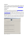
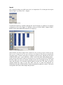
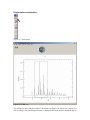
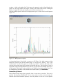
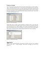
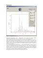
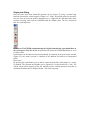
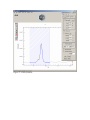
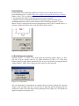
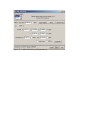
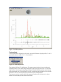
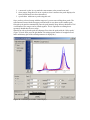
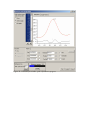
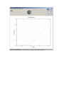
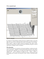
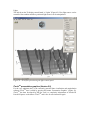
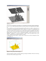
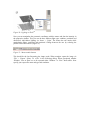
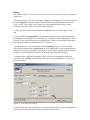
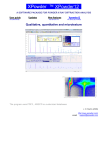
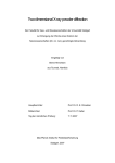
Powder3D 1.2
A short tutorial
Bernd Hinrichsen, Robert E. Dinnebier and Martin Jansen
Max Planck Institute for Solid State Research, Heisenbergstraße 1., Stuttgart, Germany
Introduction
Powder3D is a program for data reduction and publication quality visualisation aimed
specifically at large data sets collected in time resolved powder diffraction experiments. The
program is in ongoing development, so there shall be regular updates and extensions to the
present functionality. For comments or suggestions please contact [email protected] .
Getting Started
Installation
The latest version of Powder3D can be downloaded from http://www.fkf.mpg.de/xray. As
Powder3D is written in the programming language IDLTM you will need to install the IDL
virtual machine (IDL VMTM) before being able to run Powder3D.
Virtual machines for various platforms can be downloaded from the RSI website
http://www.rsinc.com/idlvm/ free of charge. When you have installed IDL VMTM unpack
Powder3D into a directory of your choice and double click on the file ‘Powder3D.sav’. After
dismissing the IDL VMTM (current version 6.3 only) splash screen the following window
(Figure 1) should welcome you.
Please note: the libraries necessary for the AVI export and peak refinement, namely
‘IDLtoAVI.dll’, ‘IDLtoAVI.dlm’, ‘p3d.dlm’ and ‘p3d.dll’ should be in the same directory as
Powder3D. The functions only work on the Windows® operating system. Other operating
systems are not supported. UNC (unmapped network) paths will cause the program to fail.
Figure 1. : Welcome screen
The sample data set
The data set that is the basis for the graphics displayed in the manual is available for
download from http://www.fkf.mpg.de/xray. The data stems from an experiment carried out at
the X7B beamline of the NSLS (Dinnebier et al., 2005). The wavelength was 0.9224 Å. The
initial substance was δ-Rb2[C2O4]. Seven phases can be identified and are tabulated below:
Table 1: Phases identified in the sample data set
Phase
SG
a/Å
b/Å
Pbam
11,29
6,29
δ-Rb2[C2O4]
6,33
10,45
P21/c
γ-Rb2[C2O4]
Pnma
8,16
6,58
β-Rb2[C2O4]
P63/mmc 6,47
α-Rb2[C2O4]
P63/mmc 5,89
α-Rb2[CO3]
Pnma
7,68
5,89
β-Rb2[CO3]
5,87
10,13
P21/c
γ-Rb2[CO3]
c/Å
3,62
8,22
10,9
8,26
7,80
10,14
7,31
β/°
98,02
97,3
Range
Æ 653K
Æ 653K
Æ 661K
Æ 723K
Æ 830K
Æ 600K
The temperature ramp was set to 298 Æ 838 Æ 298 K. The sample was heated at a rate of 2.8
Kmin-1 and cooled at a rate of 4.8 Kmin-1. Considering the exposure and development time
this leads to a heating rate of 4.2 Kframe-1 and a cooling rate of 7.62 Kframe-1.
Figure 2. : Powder diffraction patterns, lattice parameters, and cell volumes of Rb2[C2O4]
and Rb2[CO3] as a function of temperature in the range from 298 to 838 K (2.4 K min-1 and
back down to 298 K (4.8 K min-1). Taken from (Dinnebier et al., 2005).
Import
One of the first things you shall want to do is to import data. To do that press the import
button (Figure 3) or select ‘File’ > ‘Import’.
Figure 3.: Import menu
Six different formats are available, although XY and Chi formats are identical. You shall be
prompted to select a file (Figure 4). Standard versions of GSAS (GDA), Fullprof (DAT),
Bruker (UXD) and DASH (XYE) data files are imported.
Figure 4.: Select import files
Select all files you wish to import. This is different to the previous version in which you only
had to select a single file for the entire directory to be imported. The files are sorted by the
operating system, so please ensure they are displayed in the correctly. Should your files have
a different suffix, type *.<your suffix here> <Enter> in the ‘File name’ field to display them.
Upon pressing enter the file names in the directory are read, then the first file is loaded and
the theta range read. The next window prompts you for the wavelength and the two theta
range and increment. The increment entered cannot be altered later. The range can only be
cropped. Should the range of your files differ from the set values the intensities are
interpolated using the selected function: linear(recommended), quadratic or spline. The entries
correspond to the values of the sample data provided.
Figure 5.: Import settings
After the files have been read a message displays a few details on the current database (Figure
6). There is no set limit to the number of files that can be read, the only limitation is the
available memory.
Figure 6.: Import report
As soon as you acknowledge the message you are displayed the first of your powder patterns
(Figure 10).
Later pattern loading and deletion
Should you wish to load a single pattern only, or wish to compare a pattern to already loaded
data, this can be done by using the function, ‘File’ > ‘Import’ (Figure 7.). The pattern is added
to the end of the pattern array. Should the pattern differ with regard to the step width or
position the intensities are interpolated to match the range and step width of the data already
loaded. A dialog requiring you to enter the wavelength for this pattern is displayed. If one or
more patterns need to be deleted, select them in the ‘Main controls’ window and press ‘Delete
pattern’ in the ‘Edit’ menu.
Figure 8.: Adding a single pattern
Figure 9.: Pattern selection tool
Figure 10.: The first powder pattern
Data reduction
Cropping tool
The limits of the powder patterns can often be reduced. This is conveniently done by means of
the cropping tool. A click on the crop button (Figure 11) draws two vertical lines, which you
can drag to define the desired range (Figure 12).
Figure 11.: Crop button
Figure 12.: Cropping bars
On pressing the enter button the entire array is cropped to the new range.
Please note: It is a good idea to save the data regularly to avoid possible data loss. (‘File’ >
‘Save’).
Single pattern visualization
Figure 13.: Zoom button
Figure 14.: Zoom tool
The default tool in the 2D-plot window is the zoom box (Figure 14). Pull it over a region you
wish to enlarge. Once the enlarged window is displayed click in the borders around the plot to
navigate. A click to the right of the X-axis moves the pattern(s) to the left and displays the
pattern in a 2Θ region shifted 10% higher. Clicking in the other borders works in analogous
fashion. A single click in the plot window resizes it to the maximum view.
Selecting multiple patterns from the list displays them up to 6 colour coded overlaid patterns
(Figure 15).
Figure 15.: Multiple pattern display
An interesting feature is the ability to export an AVI film of the single patterns cycling
through the selected sets and the zoomed range. To do this press ‘Export > AVI’ in the
context menu. To make this export as versatile as possible it creates a film only of the
currently selected data range (2Θ, intensity and selected data sets). You will have to select an
appropriate compression algorithm for the video. In our experience DiVX4 high motion gives
the best results. This feature is only available on the Windows® operating system. Please note
the installation of the library for this function are described above (see Installation).
Normalizing Patterns
Data collected using image plates generally lacks a beam decay correction. This can be
partially alleviated by normalization. Two or more patterns can be corrected using this
function (Menu Edit>Normalize patterns). Select the patterns via the list or select patterns
belonging to a phase by choosing the appropriate phase. Next ensure the method of
normalization is correct. All patterns that have been selected are superimposed over one
another. It is possible to zoom by dragging open a zoom box with a left click. Select the
region you wish to normalize the patterns with by dragging over a range with a right click.
The range selected in this manner is used to normalize the data. By pressing ‘Test’ you can
preview the results of the normalization. Press ‘Cancel’ to discard or ‘OK’ to accept the
normalization.
Figure 16.: Normalization function
Wavelength
The wavelength dialog accessible via the menu Edit>Wavelength allows you to alter the
radiation wavelength (Figure 17). Should you wish to recalculate the pattern, select the radio
button ‘recalculate patterns’. The wavelengths for some standard anode elements have
integrated in the top list.
Figure 17.: Wavelength dialog
Phases and ranges
The increments between the patterns can be entered into a table (Figure 18) which is called by
‘Edit’ > ‘Increments and phase ranges’. For unvarying increments the fields on the right of the
window can be used to insert values into the table. Once two of the first three fields are filled
the other is calculated and filled automatically. Should all fields contain values no updating
takes place. Pressing the ‘Insert’ button fills the table with the calculated values. These values
are used for labelling purposes only.
Figure 18.: Insert increments
Adding phase ranges can either be done manually by editing the fields of the range table
(Figure 19). Please note: while editing you have to leave the cell you are editing for the values
to be read properly by the ‘Insert’ command. The assistant for entering the values at the
bottom of the window works in the same fashion as the one used in the increment window.
These values are necessary for the Le Bail assistant of which a first version is included.
Figure 19.: Define phase ranges
Kα2 stripping
Should you have collected laboratory data using Kα1 and Kα2 rays these can be separated
using the menu ‘Edit’ > ‘K-alpha stripping’. Select which wavelength you wish to keep
(Figure 20).
Figure 20.: Kα2 stripping
The following dialog (Figure 21) enables you to select the sets, which should be stripped. The
raw data is overwritten and therefore this action cannot be undone.
Figure 21.: Batch stripping
Smoothing
An advanced full width at half maximum (FWHM) optimised smoothing (Figure 22)
algorithm described by Dinnebier (Dinnebier, 2003) is implemented (‘Edit’ > ‘Smoothing’).
The variation of the FWHM of the peaks is generally described by the Caglioti (Caglioti et
al., 1958) formula:
FWHM = U tan 2 θ + V tan θ + W
This can be graphically set with aid of the function window on the left. Here the function can
be dragged to the desired shape with the aid of three red boxes.
Figure 22.: Smoothing window
The correct selection of the function shape has great effect on the smoothing efficacy.
Background
Figure 23.: Background reduction
Background determination (‘Edit’ > ‘Background’) can be done in two modes. Either a
pattern can be loaded (XY format as for import) or it can be calculated (Figure 23).
Should a pattern be loaded, it is displayed, as is the calculated background. The ‘normalize’
button then interpolates the background, giving it the same number of data points as the
diffraction pattern. Then a linear function fitted using the least absolute deviation method is
added to correct the background. Should the background be higher than the powder pattern at
any point, it is lowered.
The ‘Calculate background’ method utilises a robust algorithm based on an low-pass filter as
proposed by Sonneveld and Visser (Sonneveld & Visser, 1975). Select the number of
iterations, curvature value and number of background points to attain an optimal background.
Please note that every iteration costs computing power – for large data sets many iterations
can make the automatic background reduction time consuming.
The apply button greets you with the following dialog (Figure 24).
Figure 24.: Batch background reduction
To edit background points manually select the edit tool (Figure 25). This can become
necessary if the background varies strongly from pattern to pattern. You can now remove
background points with a shift-click (left click while pressing the shift button) and add
background points with a click.
Figure 25.: The edit tool
You can cycle through the patterns in the usual fashion, either by selecting the ‘next’ and
‘previous’ buttons in the context menu or by pressing the arrow buttons on the ‘Main’ tab. If a
background has been calculated for the pattern it will be displayed.
Should phases have been defined it is possible to select the data sets associated to the phase
by choosing the appropriate phase. The Fullprof (Rodriguez-Carvajal, 2001) format is a
simple XY ASCII file containing 2Θ values in the first column and intensities in the second.
The GSAS (Larson & Von Dreele, 1994) format contains four columns the first contains a
single ‘i’, the second contains 2Θ values, the third the intensities and the fourth the standard
errors.
Peak hunting
By selecting the menu ‘Edit’ > ’Peak search’ and clicking the search button you shall see the
following window (Figure 26). Changing the mouse to edit mode enables you to remove
peaks with a right click and add peaks with the left click. You can drag the borders of the
peak search to encompass all important areas of the powder pattern by selecting the range tool
in the context menu (right click on the image). Peaks are searched by a multiple pass, variable
FWHM, second derivative method. The convolution range is set via the Caglioti diagram, the
threshold and minimum distance between peaks can be set via the sliding bar. The radio
buttons under the Caglioti diagram determine if a new peak list is written with every run or
the current peak list appended with the newly found peaks.
Figure 26.: Peak searching
The peak positions and intensities can be saved to a Crysfire (Shirley, 2002) format file via
the button ‘Save’ on the ‘Peak search’ tab. Peaks can be added and removed manually by
selecting the ‘edit’ button as with the background points.
Single peak fitting
Once the peaks have been found their position can be (Figure 27) using a pseudo-Voigt
function corrected for axial divergence (Finger et al., 1994). All refined values are stored for
later use. You can select the peak by dragging over it. A light blue box fills the border of the
selection. Pressing enter starts the refinement with the default values. The fit is overlaid in
blue for visual inspection.
Please note: The FWHM (estimated using the Caglioti function) has a profound effect on
the convergence of the fit. Should the procedure fail ensure the FWHM distribution is set to
a realistic value.
Peak markers can be added and removed manually by returning to the peak search window
(Figure 25); the modus operandi is identical to the addition and removal of background
points.
Data export
By pressing the export button, you are able to export the peak data of the pattern in a variety
of methods. The positions and heights can be exported to Crysfire format file (*.cdt). The
refined values can be exported to text file. Should you have refined more than six peaks an
instrument resolution file (in Fullprof format *.irf) can be exported.
Figure 27.: Peak refinement
Peak Indexing
Powder3D has no own indexing capabilities, but does provide a simple interface to the
powerful indexing suite ‘Crysfire’ (http://www.ccp14.ac.uk/ccp/web-mirrors/crys-r-shirley/)
(Shirley, 2002). Two very similar methods can be chosen for interaction:
1. Save the peak file in the Crysfire format and start Crysfire manually.
2. Should Crysfire be installed (only Windows® operating systems) according to the
installation instructions in the Crysfire manual it can be called by pressing the ‘Crysfire’
button. The file is exported to the current working directory and Crysfire is started in there. A
message is displayed with the name of the file that has been exported.
Figure 28.: Crysfire button
Le Bail refinement assistant
Selecting ‘Refine’ > ‘Le Bail’ via the menu opens the following window (Figure 31). Here
you can set up the starting values for a Le Bail refinement (Le Bail et al., 1988) using
Fullprof. Should a (single pattern format) PCR file exist you can load it by pressing the button
‘Import Fullprof’. All the values displayed in the window are then imported.
Figure 29.: Le Bail menu
The cell dimensions can alternatively be imported from a Crysfire summary file. Pressing
‘Import’ in the cell frame does this. You can select a .SUM file and the cell dimensions are
displayed in a table. Select the desired cell by marking the entry (Figure 30). The lengths and
angles are imported on clicking ‘OK’.
Figure 30.: Crysfire import
The peak shape descriptors can also be imported if a peak refinement has been done for the
pattern. Otherwise enter your desired starting values (Figure 32).
The background correction is integrated into the refinement if a background was defined
using the background function.
The space group should be entered, and then you can start the refinement by pressing
‘Refine’. If the refinement is successful some statistics of the refinement are displayed at the
bottom of the window.
The button ‘Reset’ sets the phase information back to zero. The button ‘Remove HKL’
removes all HKL files for this pattern and forces Fullprof to recalculate them.
Please note: The assistant expects sequentially numbered Fullprof compatible data sets.
Please make sure that you export your patterns immediately before attempting a Le Bail
fit. All the data is written to that directory.
Figure 31.: Le Bail refinement, cell parameters
Once the refinements for all the data sets have been completed close the window by pressing
cancel. The cell dimensions can be exported to a text file by selecting the menu ‘Refine’ >
’Export cell data’.
Figure 32.: Le Bail refinement, profile parameters
Figure 33.:Le Bail refinement
Peak analysis
A new tool has been designed to assist in the sequential refinement of peak profiles. To call it
you should select the menu ‘Tool’ > ‘Peak analysis’
Figure 34.: Peak analysis menu
The window in (Figure 35.) shall appear. The pattern ranges that have been set in the main
program interface are the initial ranges displayed by the peak progression tool. It is therefore
very useful to select the interesting range using the ‘film plot’ display and the zoom function
before starting the tool. The rendering of a couple of hundred patterns might be slow on older
hardware so it is in your own interest to reduce the amount of information.
The aim was to create a module which does sequential peak profile refinement in a robust
manner. The tools that you can select on the left are
1. a zoom tool: works in very much the same manner as the normal zoom tool.
2. select ranges. Drag this tool across a peak to select it and have the peaks displayed or
found, should none have been determined.
3. a peak editor. Add/remove peaks using this tool.
Once you have selected a range with the range tool, you can start refining those peaks. The
refinement will start with the strongest peak and work its way down to the smallest peak,
fixing the peak position automatically once the peak intensity drops below a threshold of 3σI.
A maximum of two ranges can be refined together. This is equivalent to refining them
separately should there be no overlap.
Should you wish to plot the peak development, first select the peaks with the ‘Select peaks’
(Figure 36) tool. Now press the plot button The main program window is brought forward
and a rudimentary plot of the refined parameters is displayed ().
Figure 36.: Peak analysis window: initial display
Figure 37.: Peak analysis window: range selected and peaks marked
Figure 38.: Peak analysis window: peak refinement in progress
Figure 39.: Peak analysis, a rudimentary initial plot of peak development
Graphics
2D film plot
This module simulates a Guinier film (Figure 40). Two sliding bars enable you set the
brightness and contrast of the plot. Colour inversion and square root scaling can be set. A tick
box ‘Interpolate’ allows you to do a bicubic interpolation between your patterns. This
smoothes plots of small data sets. Of course the data range displayed can be set via the ‘2Θ'
and ‘Data range‘ fields. Needless to say, background corrected data has a far higher contrast.
The zoom and pan tools are available for this display.
Figure 40.: 2D-film plot
3D line (waterfall) plot
Figure 41.: 3D line plot
By clicking the 3D plot button, the default 3D line plot is displayed (Figure 41). The data
range can be set as with the 2D-film plot. Rotation around X and Y-axes can be controlled via
slides. Two preset views are stored and can be accessed via the buttons ‘Top’ and ‘Slant’.
Mouse rotation is enabled by default; pressing the appropriate radio buttons activates
translation and scaling modes. Finally the line plot can be immediately changed to a rendered
surface plot by selecting the ‘Surface’ radio button.
3D surface plot
The surface plot (Figure 42) is identical to the line plot in handling. As rendering the surface
can be a slow process – dependant on the amount data displayed, the surface mode requires
more patience while adjusting the view. All images can be exported either by copying to the
clipboard (‘Edit’ > ‘Copy’), exporting to an image file (‘File’ > ‘Export’ > ‘Image’) or
printing (‘File’ > ‘Print’). For the latter two operations the image is rendered from scratch
and, dependant on the resolution of the image file or printer, can take a considerable amount
of time.
Lights
The 2nd tab on the 3D display control board is ‘Lights’ (Figure 42). Four light sources can be
controlled. One ambient and three positional light sources can be manipulated.
Figure 42.: 3D surface plot showing the lights control panel
iToolsTM presentation graphics (Version 2.0)
For the very ambitious there is the extremely powerful data visualisation and manipulation
software iToolsTM that is called by pressing the button ‘Presentation Graphics’ (Figure 43).
iToolsTM has been developed by RSI Inc. and is a completely independent of Powder3D.
Powder3D passes on the data to iToolsTM and is free for user interaction again.
Figure 43.: iToolsTM
The iToolsTM do represent an excellent set of programmes and contain complex architecture.
For this reason, I shall extend the tutorial to cover the creation of an image like that in Figure
26.
First we shall have to subtract the background from all the data sets so that we rid ourselves of
the undulations of background intensity visible in Figure 26. A value of 1° smoothing box and
3 iterations worked well for this data set. It is convenient to decide on with part of the pattern
array you wish to use by previewing it in the 3D surface mode in Powder3D. Once you are
happy with your selection a click on ‘Presentation graphics’ copies the data over to the
iSurfaceTM programme. It is always possible to further reduce the displayed data in the
iToolsTM programme suite should you find it necessary.
A right-click on the data opens a context menu, which lets you select the properties of the
view (Figure 45).
Figure 44.:The primary iToolsTM display
Open the properties window to the full extent by pressing an unobtrusive left arrow in the top
left corner of the window (Figure 45 left).
Figure 45.: The iToolsTM property window, folded and unfolded
In the left side of ‘Visualisation Browser’ (Figure 45), You see the various elements that
make up the image. Once an element is highlighted its properties are displayed in the right
part of the window. We shall change the surface values to the following:
Color: (145,145,145), Fill shading: Gouraud, Draw method: Triangles. The last two changes
make the rendering slower, but the picture better.
We open up the ‘Axes’ branch and delete the Z-axis by a right-click and ‘delete’ (Figure 46).
Figure 46.: Deleting an element
We also alter X-axis properties to: Titel: 2Q /°, Font: Symbol
And the Y-axis to: Titel: Scan number, Font: Times
These changes give us a 2Θ on the X-axis and a similar font for the Y-axis.
Now we create that semi transparent 2D visualization hovering over the surface. Select the
menu item ‘Insert’ > ‘Visualization’ (Figure 47). You shall then be prompted for the type and
variables defining the item. We chose an ‘Image’ type (top right box), opened the ‘Surface’
branch on the left – that is where the data is – and assigned the Z-value to the pixels, Y-values
to the Y axis and X values to the X-axis. To do the assigning mark the data value on the left
and click on the small right arrow in front of the fields you wish to be associated with the
data. Leave palette empty and press ‘OK’.
So that is done, but where is the image? Find your way back to the ‘Visualization Browser’ or
properties window as described above. It shall have a new entry for the image. Highlight the
image and alter the ‘Z value’ to well above the maximum intensity in your data array. In our
case it is 85000 (Figure 49). Further set the transparency to 40.
Figure 47.: Insert visualization
Figure 48.: Define the type and variables for the visualization
Figure 49.: Correcting the height of the image
Now our image is complete. All that remains to be done is to improve the lighting and export
a high-resolution image.
You might have become aware of the ‘Lights’ branch on the left in the ‘Visualization
Browser’ (Figure 49). Open this branch and select the directional light. You should observe
something like Figure 50.
Figure 50.: Lighting in iToolsTM
Now you can manipulate the geometric coordinates with the mouse and alter the intensity in
the properties window. This you can do three different light types: ambient, positional and
directional. Add further lighting via ‘Insert’ > ‘Light’. The mouse has two modes while
manipulating lights, positional and rotational. Change between the two by selecting the
pointer or the circled arrow (Figure 51).
Figure 51.: Mouse modus buttons
This should be the last fine-tuning the image needs. When complete export the image via
‘File’ > ‘Export’. Select ‘To a file’ in the following dialog. When questioned whether
‘Window, View or Data’ are to be exported either ‘Window’ or ‘View’ shall suffice. Next
specify your export file name and type and resolution.
Recipe
This section will give you a run down on how to reduce your data sets effectively using the
sample data.
1.The data format is ‘CHI’, the wavelength is roughly 0.9184 Ångstroms. These values should
be used to import the data successfully. The temperature ramp of the experiment was 298->838-->298 K. These values can be entered into ‘Increments and phase ranges’ dialog
available via the menu ‘Edit’>’Increments and phase ranges’.
2. A first step in the data reduction would be to crop the data to a sensible range (3.4-46.7°
2Θ).
3. Next we define the background. As the background lacks great relief high values for the
smoothing box (smoothing box: 0.9, iterations: 4) – resulting in a flatter underground – do the
job well. For the data sets from 80 to 140 slightly lower values were chosen due to the higher
background at around 18°(smoothing box: 0.7, iterations: 4).
4. For the next step it is recommended to have the indexing package ‘Crysfire’ installed.
Select the first pattern and do a peak search. Save the found peaks to your working directory
and then start Crysfire, preferably by pressing the Crysfire button. Using the peak refinement
the profile can be refined and the position of the peaks determined more precisely.
5. Should you have indexed your phase(s) using Crysfire you can import them back into
Powder3D in the ‘Le Bail’ fit dialog. For this step to be successful Fullprof ( > Version 3.3)
has to be installed.
Figure 52.: Cell data for Le Bail fit
On the phase tab press import and choose a Crysfire summary file, then select the appropriate
cell from the table and the values shall be inserted into the cell fields.
Figure 53.: Import Crysfire summary file
Should you have refined profiles you can load these to the profile mask by pressing the import
button on the profile tab.
Data from an existing Fullprof file (*.pcr) can be loaded using the “Import Fullprof’ button.
On pressing “Refine” a Fullprof file is written and, should Fullprof be installed on the system,
a LeBail refinement is started. The refined data are read back to the fields.
References
When publishing please give reference to Powder3D in the following manner:
Hinrichsen, B., Dinnebier, R. E. and Jansen, M. (2004) Powder3D: An easy to use program
for data reduction and graphical presentation of large numbers of powder diffraction patterns.
Z. Krist.,23, 231-236.
Caglioti, G., Paoletti, A. & Ricci, F. P. (1958). Nucl. Instr. 3, 223-228.
Dinnebier, R. (2003). Powder DIffraction 18, 199-204.
Dinnebier, R. E., Vensky, S., Jansen, M. & Hanson, J. C. (2005). Chemistry - A European
Journal 11, 1119-1129.
Finger, L. W., Cox, D. E. & Jephcoat, A. P. (1994). Journal of Applied Crystallography 27,
892-900.
Larson, A. C. & Von Dreele, R. B. (1994). Los Alamos National Laboratory Report 86-748.
Le Bail, A., Duroy, H. & Fourquet, J. L. (1988). Mat. Res. Bull. 23, 447-452.
Rodriguez-Carvajal, J. (2001). Commission on Powder Diffraction Newsletter 26, 12-19.
Shirley, R. (2002). The Crysfire 2002 System for Automatic Powder Indexing: User's Manual.
Sonneveld, E. J. & Visser, J. W. (1975). Journal of Applied Crystallography 8, 1-7.
IDL, IDL VM and iTools are trademarks of Research Systems Inc., Boulder, CO, USA
Windows is a registered trademark of Microsoft Corporation, Redmond, WA, USA
Written by B. Hinrichsen, 06.10.2004
Last updated by B. Hinrichsen, 12.02.2007