1
CPSC 211 Data Structures & Implementations
(c) Texas A&M University [ 221]
Trees
Important terminology:
root
edge
node
parent
child
leaf
Some uses of trees:
model arithmetic expressions and other expressions
to be parsed
model game-theory approaches to solving problems:
nodes are configurations, children result from different moves
a clever implementation of priority queue ADT
search trees, each node holds a data item
CPSC 211 Data Structures & Implementations
(c) Texas A&M University [ 222]
Trees (cont’d)
Some more terms:
path: sequence of edges, each edge starts with the
node where the previous edge ends
length of path: number of edges in it
height of a node: length of longest path from the
node to a leaf
height of tree: height of root
depth (or level) of a node:
root to the node
length of path from
depth of tree: maximum depth of any leaf
Fact: The depth of a tree equals the height of the tree.
height
4
0, 3, 0
depth
0
1
2
2
0, 1
3
0
4
CPSC 211 Data Structures & Implementations
(c) Texas A&M University [ 223]
Binary Trees
Binary tree: a tree in which each node has at most two
children.
Complete binary tree: tree in which all leaves are on
the same level and each non-leaf node has exactly two
children.
Important Facts:
A complete binary tree with
nodes.
A complete binary tree with
mately levels.
levels contains nodes has approxi-
CPSC 211 Data Structures & Implementations
(c) Texas A&M University [ 224]
Binary Trees (cont’d)
Leftmost binary tree: like a complete binary tree,
except that the bottom level might not be completely
filled in; however, all leaves at bottom level are as far
to the left as possible.
Important Facts:
A leftmost
binary tree
with levels contains be
tween and nodes.
A leftmost binary tree with
mately levels.
nodes has approxi-
CPSC 211 Data Structures & Implementations
(c) Texas A&M University [ 225]
Binary Heap
Now suppose that there is a data item, called a key,
inside each node of a tree.
A binary heap (or min-heap) is a
leftmost binary tree with keys in the nodes that
satisfies the heap ordering property: every node
has a key that is less than or equal to the keys of all
its children.
Do not confuse this use of “heap” with its usage in
memory management!
Important Fact: The same set of keys can be organized in many different heaps. There is no required
order between siblings’ keys.
3
4
3
5
5
4
4
6
3
3
3
5
4
5
5
6
6
4
CPSC 211 Data Structures & Implementations
(c) Texas A&M University [ 226]
Using a Heap to Implement a Priority Queue
To implement the priority queue operation insert( ):
1. Make a new node in the tree in the next available
location, marching across from left to right.
2. Put
in the new node.
3. “Bubble up” the tree until finding a correct place:
if parent’s key, then swap keys and continue.
Time: To implement the priority queue operation remove():
Tricky part is how to remove the root without messing
up the tree structure.
1. Swap the key in the root with the key (call it ) in
the rightmost node on the bottom level.
2. Remove the rightmost node on the bottom level.
3. “Bubble down” the new root’s key until finding a
correct place: if at least one child’s key, then
swap with smallest child’s key and continue.
Time: .
CPSC 211 Data Structures & Implementations
(c) Texas A&M University [ 227]
Using a Heap to Implement a PQ (cont’d)
3
insert(2)
5
3
3
4
4
5
2
2
3
8
7
4
3
7
remove
6
8
4
5
5
4
6
2
4
4
6
7
8
PQ operation sorted array unsorted array heap
or linked list or linked
list
insert
remove (min)
No longer have the severe tradeoffs of the array and
linked list representations of priority queue. By keeping the keys “semi-sorted” instead of fully sorted, we
can decrease the tradeoff between the costs of insert
and remove.
CPSC 211 Data Structures & Implementations
(c) Texas A&M University [ 228]
Heap Sort
Recall the sorting algorithm that used a priority queue:
1. insert the elements to be sorted, one by one, into a
priority queue.
2. remove the elements, one by one, from the priority
queue; they will come out in sorted order.
If the priority queue is implemented with a heap, the
running time is .
This is much better than .
This algorithm is called heap sort.
CPSC 211 Data Structures & Implementations
(c) Texas A&M University [ 229]
Linked Structure Implementation of Heap
To implement a heap with a linked structure, each node
of the tree will be represented with an object containing
key (data)
pointer to parent node
pointer to left child
pointer to right child
To find the next available location for insert, or the
rightmost node on the bottom level for remove, in constant time, keep all nodes on the same level in a linked
list. Thus each node will also have
pointer to left neighbor on same level
pointer to right neighbor on same level
Then keep a single pointer for the whole heap that points
to the rightmost node on the bottom level.
CPSC 211 Data Structures & Implementations
(c) Texas A&M University [ 230]
Array Implementation of Heap
Fortunately, there’s a nifty way to implement a heap
using an array, based on an interesting observation: If
you number the nodes in a leftmost binary tree, starting
at the root and going across levels and down levels, you
see a pattern:
1
2
4
8
3
5
6
7
9
Node number has left child .
Node number has right child If If .
, then has no left child.
, then has no right child.
Therefore, node number is a leaf if The parent of node is , as long as Next available location for insert is index .
.
Rightmost node on the bottom level is index .
.
CPSC 211 Data Structures & Implementations
(c) Texas A&M University [ 231]
Array Implementation of Heap (cont’d)
Representation consists of
array A[1..max] (ignore location 0)
integer n, which is initially 0, holding number of
elements in heap
To implement insert(x) (ignoring overflow):
n := n+1
// make a new leaf node
A[n] := x
// new node’s key is initially x
cur := n
// start bubbling x up
parent := cur/2
while (parent != 0) && A[parent] > A[cur] do
// current node is not the root and its key
// has not found final resting place
swap A[cur] and A[parent]
cur := parent
// move up a level in the tree
parent := cur/2
endwhile
CPSC 211 Data Structures & Implementations
(c) Texas A&M University [ 232]
Array Implementation of Heap (cont’d)
To implement remove (ignoring underflow):
minKey := A[1]
// smallest key, to be returned
A[1] := A[n] // replace root’s key with key in
//
rightmost leaf on bottom level
n := n-1
// delete rightmost leaf on bottom level
cur := 1
// start bubbling down key in root
Lchild := 2*cur
Rchild := 2*cur + 1
while (Lchild <= n) && (A[minChild()] < A[cur]) do
// current node is not a leaf and its key has
// not found final resting place
swap A[cur] and A[minChild()]
cur := minChild() // move down a level in the tree
Lchild := 2*cur
Rchild := 2*cur + 1
endwhile
return minKey
minChild(): // returns index of child w/ smaller key
min := Lchild
if (Rchild <= n) && (A[Rchild] < A[Lchild]) then
// node has a right child and it is smaller
min := RChild
endif
return min
CPSC 211 Data Structures & Implementations
(c) Texas A&M University [ 233]
Binary Tree Traversals
Now consider any kind of binary tree with data in the
nodes, not just leftmost binary trees.
In many applications, we need to traverse a tree: “visit”
each node exactly once. When the node is visited,
some computation can take place, such as printing the
key.
There are three popular kinds of traversals, differing in
the order in which each node is visited in relation to the
order in which its left and right subtrees are visited:
inorder traversal: visit the node IN between visiting the left subtree and visiting the right subtree
preorder traversal: visit the node BEFORE visiting either subtree
postorder traversal: visit the node AFTER visiting both its subtrees
In all cases, it is assumed that the left subtree is visited
before the right subtree.
CPSC 211 Data Structures & Implementations
(c) Texas A&M University [ 234]
Binary Tree Traversals (cont’d)
preorder(x):
if x is not empty then
visit x
preorder(leftchild(x))
preorder(rightchild(x))
inorder(x):
if x is not empty then
inorder(leftchild(x))
visit x
inorder(rightchild(x))
postorder(x):
if x is not empty then
postorder(leftchild(x))
postorder(rightchild(x))
visit x
a
b
c
f
d
e
preorder: a b d e c f g h i
inorder: d e b a f c h g i
postorder: e d b f h i g c
g
h
i
CPSC 211 Data Structures & Implementations
(c) Texas A&M University [ 235]
Binary Tree Traversals (cont’d)
These traversals are particularly interesting when the
binary tree is a parse tree for an arithmetic expression:
Postorder traversal results in the postfix representation of the expression.
Preorder gives prefix representation.
Does inorder give infix? No, because there are no
parentheses to indicate precedence.
*
+
5
3
preorder: * + 5 3 - 2 1
inorder: 5 3 + 2 1 - *
postorder: 5 + 3 * 2 - 1
2
1
CPSC 211 Data Structures & Implementations
(c) Texas A&M University [ 236]
Representation of a Binary Tree
The most straightforward representation for an (arbitrary) binary tree is a linked structure, where each node
has
key
pointer to right child
pointer to left child
Notice that the array representation used for a heap
will not work, because the structure of the tree is not
necessarily very regular.
class TreeNode {
Object data;
TreeNode left;
TreeNode right;
// data in the node
// left child
// right child
// constructor goes here...
void visit() {
// what to do when node is visited
}
}
CPSC 211 Data Structures & Implementations
(c) Texas A&M University [ 237]
Representation of a Binary Tree (cont’d)
class Tree {
TreeNode root;
// other information...
void preorderTraversal() {
preorder(root);
}
preorder(TreeNode t) {
if (t != null) {
// stopping case for recursion
t.visit();
// user-defined visit method
preorder(t.left);
preorder(t.right);
}
}
}
But we haven’t yet talked about how you actually MAKE
a binary tree. We’ll do that next, when we talk about
binary SEARCH trees.
CPSC 211 Data Structures & Implementations
(c) Texas A&M University [ 238]
Dictionary ADT Specification
So far, we’ve seen the abstract data types
priority queue, with operations insert, remove (min),...
stack, with operations push, pop,...
queue, with operations enq, deq,...
list, with operations insert, delete, replace,...
Another useful ADT is a dictionary (or table). The
abstract state of a dictionary is a set of elements, each
of which has a key. The main operations are:
insert an element
delete an arbitrary element (not necessarily the highest priority one)
search for a particular element
Some additional operations are:
find the minimum element,
find the maximum element,
print out all elements in sorted order.
CPSC 211 Data Structures & Implementations
(c) Texas A&M University [ 239]
Dictionary ADT Applications
The dictionary (or table) ADT is useful in “database”
type applications.
For instance, student records at a university can be kept
in a dictionary data structure:
When a new student enrolls, an insert is done.
When a student graduates, a delete is done.
When information about a student needs to be updated, a search is done, using either the name or ID
number as the key.
Once the search has located the record for that student, the data can be updated.
When information about student needs to be retrieved,
a search is done.
The world is full of information databases, many of
them extremely large (imagine what the IRS has).
When the number of elements gets very large, efficient
implementations of the dictionary ADT are essential.
CPSC 211 Data Structures & Implementations
(c) Texas A&M University [ 240]
Dictionary Implementations
We will study a number of implementations:
Search Trees
(basic) binary search trees
balanced search trees
– AVL trees (binary)
– red-black trees (binary)
– B-trees (not binary)
tries (not binary)
Hash Tables
open addressing
chaining
CPSC 211 Data Structures & Implementations
(c) Texas A&M University [ 241]
Binary Search Tree
Recall the heap ordering property for binary heaps:
each node’s key is smaller than the keys in both children.
Another ordering property is the binary search tree
property: for each node ,
all keys in the left subtree of
in , and
are less than the key
all keys in the right subtree of
key in .
are greater than the
A binary search tree (BST) is a binary tree that satisfies the binary search tree property.
19
10
4
22
16
13
20
17
26
27
CPSC 211 Data Structures & Implementations
(c) Texas A&M University [ 242]
Searching in a BST
To search for a particular key in a binary search tree,
we take advantage of the binary search tree property:
search(x,k): // x is node where search starts
----------- // k is key searched for
if x is null then
// stopping case for recursion
return "not found"
else if k = the key of x then
return x
else if k < the key of x then
search(leftchild(x),k)
// recursive call
else // k > the key of x
search(rightchild(x),k)
// recursive call
endif
The top level call has
equal to the root of the tree.
In the previous tree, the search path for 17 is 19, 10,
16, 17, and the search path for 21 is 19, 22, 20, null.
Running Time: , where
BST is a chain, then
.
is depth of tree.
If
CPSC 211 Data Structures & Implementations
(c) Texas A&M University [ 243]
Searching in a BST (cont’d)
Iterative version of search:
search(x,k):
-----------while x != null do
if k = the key of x then
return x
else if k < the key of x then
x := leftchild(x)
else // k > the key of x
x := rightchild(x)
endif
endwhile
return "not found"
As in the recursive version, you keep going down the
tree until you either find the key or hit a leaf.
The comparison of the search key with the node key
tells you at each level whether to continue the search
to the left or to the right.
Running Time: .
CPSC 211 Data Structures & Implementations
(c) Texas A&M University [ 244]
Searching in a Balanced BST
If the tree is a complete binary tree, then the depth is
, and thus the search time is .
Binary trees with depth are considered balanced: there is balance between the number of nodes
in the left subtree and the number of nodes in the right
subtree of each node.
You can have binary trees that are approximately balanced, so that the depth is still , but might have
a larger constant hidden in the big-oh.
As an aside, a binary heap does not have an efficient
search operation: Since nodes at the same level of the
heap have no particular ordering relationship to each
other, you will need to search the entire heap in the
worst case, which will be time, even though the
tree is perfectly balanced and only has depth .
CPSC 211 Data Structures & Implementations
(c) Texas A&M University [ 245]
Inserting into a BST
To insert a key into a binary search tree, search starting at the root until finding the place where the key
should go. Then link in a node containing the key.
insert(x,k):
----------if x = null then
make a new node containing k
return new node
else if k = the key of x then
return null // key already exists
else if k < the key of x then
leftchild(x) := insert(leftchild(x),k)
return x
else // k > the key of x
rightchild(x) := insert(rightchild(x),k)
return x
endif
Insert called on node returns node , unless is null,
in which case insert returns a new node. As a result, a
child of a node is only changed if it is originally nonexistent.
Running Time: .
CPSC 211 Data Structures & Implementations
(c) Texas A&M University [ 246]
Inserting into a BST (cont’d)
19
10
4
22
16
20
26
27
17
13
after inserting 2, then 18, then 21:
19
10
4
2
22
20
16
13
17
26
21
18
27
CPSC 211 Data Structures & Implementations
(c) Texas A&M University [ 247]
Finding Min and Max in Binary Search Tree
Fact: The smallest key in a binary tree is found by
following left children as far as you can.
19
10
4
22
16
13
20
27
17
Running Time: 26
.
Guess how to find the largest key and how long it takes.
Min is 4 and max is 27.
CPSC 211 Data Structures & Implementations
(c) Texas A&M University [ 248]
Printing a BST in Sorted Order
Cute tie-in between tree traversals and BST’s.
Theorem: Inorder traversal of a binary search tree visits the nodes in sorted order of the keys.
Inorder traversal on previous tree gives: 4, 10, 13, 16,
17, 19, 20, 22, 26, 27.
Proof: Let’s look at some small cases and then use
induction for the general case.
Case 1: Single node. Obvious.
Case 2: Two nodes. Check the two cases.
Case : Suppose true for trees of size 1 through Consider a tree of size :
.
CPSC 211 Data Structures & Implementations
(c) Texas A&M University [ 249]
Printing a BST in Sorted Order (cont’d)
r
R
all keys
greater than r
L
all keys
less than r
contains
at most keys.
keys, and
contains at most
Inorder traversal:
prints out all keys in
in sorted order, by induction.
then prints out key in , which is larger than all keys
in ,
then prints out all keys in in sorted order, by induction. All these keys are greater than key in .
Running Time: since each node is handled once.
CPSC 211 Data Structures & Implementations
(c) Texas A&M University [ 250]
Tree Sort
Does previous theorem suggest yet another sorting algorithm to you?
Tree Sort: Insert all the keys into a BST, then do an
inorder traversal of the tree.
Running Time: takes time.
, since each of the
inserts
CPSC 211 Data Structures & Implementations
(c) Texas A&M University [ 251]
Finding Successor in a BST
The successor of a node in a BST is the node whose
key immediately follows ’s key, in sorted order.
Case 1: If has a right child, then the successor of
is the minimum in the right subtree: follow ’s right
pointer, then follow left pointers until there are no more.
19
10
4
22
16
13
20
17
26
27
Path to find successor of 19 is 19, 22, 20.
CPSC 211 Data Structures & Implementations
(c) Texas A&M University [ 252]
Finding Successor in a BST (cont’d)
19
10
4
22
16
20
17
13
26
27
Case 2: If does not have a right child, then find the
lowest ancestor of whose left child is also an ancestor
of . (I.e., follow parent pointers from until reaching
a key larger than ’s.)
Path to find successor of 17 is 17, 16, 10, 19.
If you never find an ancestor that is larger than ’s key,
then was already the maximum and has no successor.
Path to try to find successor of 27 is 27, 26, 22, 19.
Running Time: .
CPSC 211 Data Structures & Implementations
(c) Texas A&M University [ 253]
Finding Predecessor in a BST
The predecessor of a node in a BST is the node
whose key immediately precedes ’s key, in sorted order. To find it, do the “mirror image” of the algorithm
for successor.
Case 1: If has a left child, then the predecessor of is
the maximum in the left subtree: follow ’s left pointer,
then follow right pointers until there are no more.
Case 2: If does not have a left child, then find the
lowest ancestor of whose right child is also an ancestor of . (I.e., follow parent pointers from until
reaching a key smaller than ’s.)
If you never find an ancestor that is smaller than ’s
key, then was already the minimum and has no predecessor.
Running Time: .
CPSC 211 Data Structures & Implementations
(c) Texas A&M University [ 254]
Deleting a Node from a BST
Case 1:
tree.
is a leaf. Then just delete ’s node from the
Case 2: has only one child. Then “splice out”
connecting ’ parent directly to ’s (only) child.
by
Case 3: has two children. Use the same strategy as
binary heap: Instead of removing the root node, choose
another node that is easier to remove, and swap the data
in the nodes.
1. Find the successor (or predecessor) of , call it . It
is guaranteed to exist since has two children.
2. Delete from the tree. Since is the successor, it
has no left child, and thus it can be dealt with using
either Case 1 or Case 2.
3. Replace ’s key with ’s key.
Running Time: .
CPSC 211 Data Structures & Implementations
(c) Texas A&M University [ 255]
Deleting a Node from a BST (cont’d)
19
10
4
22
16
20
26
27
17
13
after deleting 13, then 26, then 10:
19
16
4
22
17
20
27
CPSC 211 Data Structures & Implementations
(c) Texas A&M University [ 256]
Balanced Search Trees
We would like to come up with a way to keep a binary
search tree “balanced”, so that the depth is ,
and thus the running time for the BST operations will
be , instead of .
There are a number of schemes that have been devised.
We will briefly look at a few of them.
They all require much more complicated algorithms
for insertion and deletion, in order to make sure that
the tree stays balanced.
The algorithms for searching, finding min, max, predecessor or successor, are essentially the same as for the
basic BST.
Next few slides give the main idea for the definitions
of the trees, but not why the definitions give depth, and not how the algorithms for insertion and
deletion work.
CPSC 211 Data Structures & Implementations
(c) Texas A&M University [ 257]
AVL Trees
An AVL tree is a binary search tree such that for each
node, the heights of the left and right subtrees of the
node differ by at most 1.
3
1
0
1
0
5
2
2
2
0
7
1
3
0
1 0
4
6
0
0
0
.
Theorem: The depth of an AVL tree is When inserting or deleting a node in an AVL tree, if
you detect that the AVL tree property has been violated, then you rearrange the shape of the tree using
“rotations”.
CPSC 211 Data Structures & Implementations
(c) Texas A&M University [ 258]
Red-Black Trees
A red-black tree is a binary search tree in which
every “real” node is given 0, 1 or 2 “fake” NIL
children to ensure that it has two children and
every node is colored either red or black s.t.:
– every leaf node is black,
– if a node is red, then both its children are black,
– every path from a node to a leaf contains the same
number of black nodes 3
2 7 N 1
3
N 2
N 14
16
10
12
2
N N 1
N 15
N
2
N From a fixed node, all paths from that node to a leaf
differ in length by at most a factor of 2, implying
Theorem: The depth of an AVL tree is .
Insert and delete algorithms are quite involved.
CPSC 211 Data Structures & Implementations
(c) Texas A&M University [ 259]
B-Trees
The AVL tree and red-black tree allowed some variation in the lengths of the different root-to-leaf paths.
An alternative idea is to make sure that all root-to-leaf
paths have exactly the same length and allow variation
in the number of children.
The definition of a B-tree uses a parameter
:
every leaf has the same depth
the root has at most
children
every non-root node has from
to
children
Keys are placed into nodes like this:
Each non-leaf node has one fewer keys than it has
children. Each key is “between” two child pointers.
Each leaf node has between
and
keys
in it (unless it is also
the root, in which case it has
between 1 and
keys in it).
The keys within a node are listed in increasing order.
CPSC 211 Data Structures & Implementations
(c) Texas A&M University [ 260]
B-Trees (cont’d)
And we require the extended search tree property:
For each node , the -th key in is larger than all
the keys in ’s -th subtree and is smaller than all
-st subtree
the keys in ’s 13
2
3
4
8
6
7
17 20
10
11 12
14
16
18
19
24
22
23
25 26
B-trees are extensively used in the real world, for instance, database applications. In practice,
is very
large (such as 512 or 1024).
.
Theorem: The depth of a B-tree tree is Insert and delete algorithms are quite involved.
CPSC 211 Data Structures & Implementations
(c) Texas A&M University [ 261]
Tries
In the previous search trees, each key is independent
of the other keys in the tree, except for their relative
positions.
For some kinds of keys, one key might be a prefix of
another tree. For example, if the keys are strings, then
the key “at” is a prefix of the key “atlas”.
The next kind of tree takes advantage of prefix relationships between keys to store them more efficiently.
A trie is a (not necessarily binary) tree in which
each node corresponds to a prefix of a key, and
prefix for each node extends prefix of its parent.
The trie storing “a”, “ ale”, “ant”, “bed”, “bee”, “bet”:
a
b
l
e
n
t
e
d e
t
CPSC 211 Data Structures & Implementations
(c) Texas A&M University [ 262]
Inserting into a Trie
To insert into a trie:
insert(x,s): // x is node, s is string to insert
-----------if length(s) = 0 then
mark x as holding a complete key
else
c := first character in s
if no outgoing edge from x is labeled with c then
create a new child node of x
label the edge to the new child node with c
put the edge in the correct sorted order
among all of x’s outgoing edges
endif
x := child of x reached by edge labeled c
s := result of removing first character from s
insert(x,s)
endif
Start the recursion with the root.
To insert “an” and “beep”:
a
b
l
e
n
t
e
d e
t
CPSC 211 Data Structures & Implementations
(c) Texas A&M University [ 263]
Searching in a Trie
To search in a trie:
search(x,s): // x is node, s is string to search for
-----------if length(s) = 0 then
if x holds a complete key then return x
else return null // s is not in the trie
else
c := first character in s
if no outgoing edge from x is labeled with c then
return null // s is not in the trie
else
x := child of x reached by edge labeled c
s := result of removing first character from s
search(x,s)
endif
endif
Start the recursion with the root.
To search for “art” and “bee”:
a
b
l
e
n
t
e
d e
t
CPSC 211 Data Structures & Implementations
(c) Texas A&M University [ 264]
Hash Table Implementation of Dictionary ADT
Another implementation of the Dictionary ADT is a
hash table.
Hash tables support the operations
insert an element
delete an arbitrary element
search for a particular element
with constant average time performance. This is a
significant advantage over even balanced search trees,
which have average times of .
The disadvantage of hash tables is that the operations
min, max, pred, succ take time; and printing all
elements in sorted order takes time.
CPSC 211 Data Structures & Implementations
(c) Texas A&M University [ 265]
Main Idea of Hash Table
Main idea: exploit random access feature of arrays:
the i-th entry of array A can be accessed in constant
time, by calculating the address of A[i], which is offset
from the starting address of A.
Simple example: Suppose all keys are in the range 0
to 99. Then store elements in an array A with 100
entries. Initialize all entries to some empty indicator.
To insert x with key k: A[k] := x.
To search for key k: check if A[k] is empty.
To delete element with key k: A[k] := empty.
All times are .
0
x0
1
key is 0
2
x2
...
key is 2
But this idea does not scale well.
99
x99
key is 99
CPSC 211 Data Structures & Implementations
(c) Texas A&M University [ 266]
Hash Functions
Suppose
elements are student records
school has 40,000 students,
keys are social security numbers (000-00-0000).
Since there are 1 billion possible SSN’s, we need an
array of length 1 billion. And most of it will be wasted,
since only 40,000/1,000,000,000 = 1/25,000 fraction is
nonempty.
Instead, we need a way to condense the keys into a
smaller range.
Let
be the size of the array we are willing to provide.
Use a hash function, , to convert each key to an array
index. Then
maps key values to integers in the range
0 to
.
CPSC 211 Data Structures & Implementations
(c) Texas A&M University [ 267]
Simple Hash Function Example
Suppose keys are integers. Let the hash function be
. Notice that this
always gives you
something in the range 0 to
(an array index).
To insert
with key :
To search for element with key : check if is empty
To delete element with key : set to empty.
All times are , assuming the hash function can be
computed in constant time.
0
1
2
x
99
...
key is k and h(k) = 2
The key to making this work is to choose hash function
and table size
properly (they interact).
CPSC 211 Data Structures & Implementations
(c) Texas A&M University [ 268]
Collisions
In reality, any hash function will have collisions: when
two different keys hash to the same value:
, although
.
This is inevitable, since the hash function is squashing
down a large domain into a small range.
For example, if , then
collide since they both hash to 0 (
0, and
is also 0).
and
is
What should you do when you have a collision? Two
common solutions are
1. chaining, and
2. open addressing
CPSC 211 Data Structures & Implementations
(c) Texas A&M University [ 269]
Chaining
Keep all data items that hash to the same array location
in a linked list:
0
1
2
all have keys that hash to 1
.
.
.
M-1
to insert element
of linked list at with key : put
at beginning
to search for element with key : scan the linked
list at for an element with key
to delete element with key : do search, if search is
successful then remove element from the linked list
Worst case times, assuming computing
is constant:
insert: .
search and delete: . Worst case is if all
ments hash to same location.
ele-
CPSC 211 Data Structures & Implementations
(c) Texas A&M University [ 270]
Good Hash Functions for Chaining
Intuition: Hash function should spread out the data
evenly among the
entries in the table.
More formally: any key should be equally likely to
hash to any of the
locations.
Impractical to check in practice since the probability
distribution on the keys is usually not known.
For example: Suppose the symbol table in a compiler
is implemented with a hash table. The compiler writer
cannot know in advance which variable names will appear in each program to be compiled.
Heuristics are used to approximate this condition: try
something that seems reasonable, and run some experiments to see how it works.
CPSC 211 Data Structures & Implementations
(c) Texas A&M University [ 271]
Good Hash Functions for Chaining (cont’d)
Some issues to consider in choosing a hash function:
Exploit application-specific information. For symbol table example, take into account the kinds of
variables names that people often choose (e.g., x1).
Try to avoid collisions on these names.
Hash function should depend on all the information
in the keys. For example: if the keys are English
words, it is not a good idea to hash on the first letter,
since many words begin with S and few with X.
CPSC 211 Data Structures & Implementations
(c) Texas A&M University [ 272]
Average Case Analysis of Chaining
Define load factor of hash table with
entries and keys to be
. (How full the table is.)
Assume a hash function that is ideal for chaining (any
key is equally likely to hash to any of the
locations).
Fact: Average length of each linked list is .
The average running time for chaining:
Insert: (same as worst case).
. time to comUnsuccessful Search: pute ; items, on average, in the linked list are
checked until discovering that is not present.
Successful Search: . time to compute ; on average, key being sought is in middle
of linked list, so comparisons needed to find .
Delete: Essentially the same as search.
For these times to be , must be , so cannot
be too much larger than .
CPSC 211 Data Structures & Implementations
(c) Texas A&M University [ 273]
Open Addressing
With this scheme, there are no linked lists. Instead, all
elements are stored in the table proper.
If there is a collision, you have to probe the table –
check whether a slot (table entry) is empty – repeatedly
until finding an empty slot.
You must pick a pattern that you will use to probe the
table.
The simplest
pattern is to start at and then check
, , , wrapping around to
,
check 0, 1, 2, etc. if necessary, until finding an empty
slot. This is called linear probing.
0
1
2
F
F
F
3
4
5
F
F
6
7
8
F
F
If , the probe sequence will be 7, 8, 0, 1, 2, 3.
(F means full.)
CPSC 211 Data Structures & Implementations
(c) Texas A&M University [ 274]
Clustering
A problem with linear probing: clusters can build up.
A cluster is a contiguous group of full slots.
If an insert probe sequence begins in a cluster,
it takes a while to get out of the cluster to find an
empty slot,
then inserting the new element just makes the cluster even bigger.
To reduce clustering, change the probe increment to
skip over some locations, so locations are not checked
in linear order.
There are various schemes for how to choose the increments; in fact, the increment to use can be a function
of how many probes you have already done.
CPSC 211 Data Structures & Implementations
(c) Texas A&M University [ 275]
Clustering (cont’d)
0
1
2
F
F
F
3
4
5
F
F
6
7
8
F
F
If the probe sequence starts at 7 and the probe increment is 4, then the probe sequence will be 7, 2, 6.
Warning! The probe increment must be relatively prime
to the table size (meaning that they have no common
factors): otherwise you will not search all locations.
For example, suppose you have table size 9 and increment 3. You will only search 1/3 of the table locations.
CPSC 211 Data Structures & Implementations
(c) Texas A&M University [ 276]
Double Hashing
Even when “non-linear” probing is used, it is still true
that two keys that hash to the same location will follow
the same probe sequence.
To get around this problem, use double hashing:
1. One hash function,
to start probing.
, is used to determine where
2. A second hash function,
probe sequence.
, is used to determine the
If the hash functions are chosen properly, different keys
that have the same starting place will have different
probe increments.
CPSC 211 Data Structures & Implementations
(c) Texas A&M University [ 277]
Double Hashing Example
Let
0
1
79
2
3
and
4
69
5
98
6
7
72
8
9
15
To insert 14: start probing at
increment is
is 1, 5, 9, 0.
To insert 27: start probing at increment is
is 1, 7, 0, 6.
10
11
50
.
12
. Probe
. Probe sequence
. Probe
. Probe sequence
To search for 18: start
at
probing
Probe increment is
sequence is 5, 0 – not in table.
.
. Probe
CPSC 211 Data Structures & Implementations
(c) Texas A&M University [ 278]
Deleting with Open Addressing
Open addressing has another complication:
to insert: probe until finding an empty slot.
to search: probe until finding the key being sought
or an empty slot (which means not there)
Suppose we use linear probing. Consider this sequence:
Insert
Insert
Insert
Delete
empty.
, where , where , where , at location 3.
, at location 4.
, at location 5.
from location 4 by setting location 4 to
Search for . Incorrectly stops searching at location 4 and declares not in the table!
Solution: when an element is deleted, instead of marking the slot as empty, it should be marked in a special
way to indicate that an element used to be there but was
deleted. Then the search algorithm needs to continue
searching if it finds one of those slots.
CPSC 211 Data Structures & Implementations
(c) Texas A&M University [ 279]
Good Hash Functions for Open Addressing
An ideal hash function for open addressing would satisfy an even stronger property than that for chaining,
namely:
Each key should be equally
likely to have each per
mutation of
as its probe sequence.
This is even harder to achieve in practice than the ideal
property for chaining.
A good approximation is double hashing with this scheme:
Let
be prime, then let
.
Generalizes the earlier example.
and let
CPSC 211 Data Structures & Implementations
(c) Texas A&M University [ 280]
Average Case Analysis of Open Addressing
In this situation, the load factor
is always
less than 1: there cannot be more keys in the table than
there are table entries, since keys are stored directly in
the table.
Assume that there is always at least one empty slot.
Assume that the hash function ensures that each key is
equally
likely tohave
each permutation of
as its probe sequence.
Average case running times:
Unsuccessful Search: .
Insert: Essentially same as unsuccessful search.
Successful Search: ).
natural log (base , where is the
Delete: Essentially same as search.
The reasoning behind these formulas requires more sophisticated probability than for chaining.
CPSC 211 Data Structures & Implementations
(c) Texas A&M University [ 281]
Sanity Check for Open Addressing Analysis
The time for searches should increase as the load factor
increases.
The formula for unsuccessful search is As gets closer to
,
so
.
gets closer to 1,
gets closer to 0,
so
gets larger.
, the formula
At the extreme, when , meaning that you will search the entire table before
discovering that the key is not there.
CPSC 211 Data Structures & Implementations
(c) Texas A&M University [ 282]
Sorting
Insertion Sort:
– Consider each element in the array, starting at the
beginning.
– Shift the preceding, already sorted, elements one
place to the right, until finding the proper place
for the current element.
– Insert the current element into its place.
– Worst-case time is .
Treesort:
– Insert the items one by one into a binary search
tree.
– Then do an inorder traversal of the tree.
– For a basic BST, worst-case time is , but
average time is .
– For a balanced BST, worst-cast time is ,
although code is more complicated.
CPSC 211 Data Structures & Implementations
(c) Texas A&M University [ 283]
Sorting (cont’d)
Heapsort:
– Insert the items one by one into a heap.
– Then remove the minimum element one by one.
Elements will come out in sorted order.
– Worst-case time is .
Mergesort: Apply the idea of divide and conquer:
– Split the input array into half.
– Recursively sort the first half.
– Recursively sort the second half.
– Then merge the two sorted halves together.
– Worst-case time is like heapsort; however, it requires more space.
CPSC 211 Data Structures & Implementations
(c) Texas A&M University [ 284]
Object-Oriented Software Engineering
References:
Standish textbook, Appendix C
Developing Java Software, by Russel Winder and
Graham Roberts, John Wiley & Sons, 1998 (ch 89).
Outline of material:
Introduction
Requirements
Object-oriented analysis and design
Verification and correctness proofs
Implementation
Testing and debugging
Maintenance and documentation
Measurement and tuning
Software reuse
CPSC 211 Data Structures & Implementations
(c) Texas A&M University [ 285]
Small Scale vs. Large Scale Programming
Programming in the small: programs done by one
person in a few hours or days, whose length is just a
few pages (typically under 1000 lines of code).
Programming in the large: projects consisting of many
people, taking many months, and producing thousands
of lines of code. Obviously the complications are much
greater here.
The field of software engineering is mostly oriented
toward how to do programming in the large well. However, the principles still hold (although simplified) for
programming in the small. It’s worth understanding
these principles so that
you can write better small programs and
you will have a base of understanding for when you
go on to large programs.
CPSC 211 Data Structures & Implementations
(c) Texas A&M University [ 286]
Object-Oriented Software Engineering
Software engineering studies how to define, design,
implement and maintain software systems.
Object-oriented software engineering uses notions
of classes, objects and inheritance to achieve these goals.
Why object-oriented?
use of abstractions to control complexity, focus on
one subproblem at a time
benefits of encapsulation to prevent unwanted side
effects
power of inheritance to reuse sofware
Experience has shown that object-oriented software engineering
helps create robust reliable programs with clean designs and
promotes the development of programs by combining existing components.
CPSC 211 Data Structures & Implementations
(c) Texas A&M University [ 287]
Object-Oriented Software Engineering (cont’d)
Solutions to specific problems tend to be fragile and
short-lived: any change to the requirements can result
in massive revisions.
To minimize effects of requirement changes capture
general aspects of the problem domain (e.g., student
record keeping at a university) instead of just focusing
on how to solve a specific problem (e.g., printing out
all students in alphabetical order.)
Usually the problem domain is fairly stable, whereas a
specific problem can change rapidly.
If you capture the problem domain as the core of
your design, then the code is likely to be more stable, reusable and adaptable.
More traditional structured programming tends to lead
to a strictly top-down way of creating programs, which
then have rigid structure and centralized control, and
thus are difficult to modify.
CPSC 211 Data Structures & Implementations
(c) Texas A&M University [ 288]
Object-Oriented Software Engineering (cont’d)
In OO analysis and design,identify the abstractions needed
by the program and model them as classes. Leads to
middle-out design:
go downwards to flesh out the details of how to
implement the classes
go upwards to relate the classes to each other, including inheritance relationships, and use the classes
to solve the problem
This approach tends to lead to decentralized control
and programs that are easier to change. For instance,
when the requirements change, you may have all the
basic abstractions right but you just need to rearrange
how they interact.
Aim for a core framework of abstract classes and
interfaces representing the core abstractions, which
are specialized by inheritance to provide concrete
classes for specific problems.
CPSC 211 Data Structures & Implementations
(c) Texas A&M University [ 289]
Software Life Cycle
inception: obtain initial ideas
– requirements: gather information from the user
about the intended and desired use
elaboration: turn requirements into a specification
that can be implemented as a program
– analysis: identify key abstractions, classes and
relationships
– design: refine your class model to the point where
it can be implemented
– identify reuse: locate code that can be reused
implementation
– program and test each class
– integrate all the classes together
– make classes and components reusable for the
future
testing
delivery and maintenance
CPSC 211 Data Structures & Implementations
(c) Texas A&M University [ 290]
Software Life Cycle (cont’d)
Lifecycle is not followed linearly; there is a great deal
of iteration.
An ideal way to proceed is by iterative prototyping:
implement a very simple, minimal version of your
program
review what has been achieved
decide what to do next
proceed to next iteration of implementation
continue iterating until reaching final goal
This supports exploring the design and implementation
incrementally, letting you try alternatives and correct
mistakes before they balloon.
CPSC 211 Data Structures & Implementations
(c) Texas A&M University [ 291]
Requirements
Decide what the program is supposed to do before starting to write it. Harder than it sounds.
Ask the user
what input is needed
what output should be generated
Involve the user in reviewing the requirements when
they are produced and the prototypes developed.
Typically, requirements are organized as a bulleted list.
Helpful to construct scenarios, which describe a sequence of steps the program will go through, from the
point of view of the user, to accomplish some task.
CPSC 211 Data Structures & Implementations
(c) Texas A&M University [ 292]
Requirements (cont’d)
An example scenario to look up a phone number:
1. select the find-phone-number option
2. enter name of company whose phone number is desired
3. click search
4. program computes, to find desired number (do NOT
specify data structure to be used at this level)
5. display results
Construct as many scenarios as needed until you feel
comfortable, and have gotten feedback from the user,
that you’ve covered all the situations.
This part of the software life cycle is no different for
object-oriented software engineering than for non-objectoriented.
CPSC 211 Data Structures & Implementations
(c) Texas A&M University [ 293]
Object-Oriented Analysis and Design
Main objective: identify the classes that will be used
and their relationships to each other.
Analysis and design are two ends of a spectrum: Analysis focuses more on the real-world modeling, while
design focuses more on the programming aspects.
For large scale projects, there might be a real distinction: for example, several programming-level classes
might be required to implement a real-world level “class”.
For small scale projects, there is typically no distinction between analysis and design: we can directly figure out what classes to have in the program to solve the
real-world problem.
CPSC 211 Data Structures & Implementations
(c) Texas A&M University [ 294]
Object-Oriented Analysis and Design (cont’d)
To decide on the classes:
Study the requirements, brainstorming and using common sense.
Look for nouns in the requirements: names, entitites, things (e.g., courses, GPAs, names), roles
(e.g., student), even strategies and abstractions.
These will probably turn into classes (e.g., student,
course) and/or instance variables of classes (e.g.,
GPA, name).
See how the requirements specify interactions between things (e.g., each student has a GPA, each
course has a set of enrolled students).
Use an analysis method: a collection of notations
and conventions that supposedly help people with
the analysis, design, and implementation process.
(Particularly aimed at large scale projects.)
CPSC 211 Data Structures & Implementations
(c) Texas A&M University [ 295]
An Example OO Analysis Method
CRC (Class, Responsibility, Collaboration): It clearly
identifies the Classes, what the Responsibilities are of
each class, and how the classes Collaborate (interact).
In the CRC method, you draw class diagrams:
each class is indicated by a rectangle containing
– name of class
– list of attributes (instance variables)
– list of methods
if class 1 is a subclass of class 2, then draw an arrow
from class 1 rectangle to class 2 rectangle
if an object of class 1 is part of (an instance variable
of) class 2, then draw a line from class 1 rectangle
to class 2 rectangle with a diamond at end.
if objects of class 1 need to communicate with objects of class 2, then draw a plain line connecting
the two rectangles.
The arrows and lines can be annotated to indicate the
number of objects involved, the role they play, etc.
CPSC 211 Data Structures & Implementations
(c) Texas A&M University [ 296]
CRC Example
To model a game with several players who take turns
throwing a cup containing dice, in which some scoring
system is used to determine the best score:
Game
Die
players
value
playGame()
throw()
getValue()
Player
Cup
name
score
dice
playTurn()
getScore()
throwDice()
getValue()
This is a diagram of the classes, not the objects. Object diagrams are trickier since objects come and go
dynamically during execution.
Double-check that the class diagram is consistent with
requirements scenarios.
CPSC 211 Data Structures & Implementations
(c) Texas A&M University [ 297]
Object-Oriented Analysis and Design (cont’d)
While fleshing out the design, after identifying what
the different methods of the classes should be, figure
out how the methods will work.
This means deciding what algorithms and associated
data structures to use.
Do not fall in love with one particular solution (such
as the first one that occurs to you). Generate as many
different possible solutions as is practical, and then try
to identify the best one.
Do not commit to a particular solution too early in the
process. Concentrate on what should be done, not how,
until as late as possible. The use of ADTs assists in this
aspect.
CPSC 211 Data Structures & Implementations
(c) Texas A&M University [ 298]
Verification and Correctness Proofs
Part of the design includes deciding on (or coming up
with new) algorithms to use.
You should have some convincing argument as to why
these algorithms are correct.
In many cases, it will be obvious:
trivial action, such as a table lookup
using a well known algorithm, such as heap sort
But sometimes you might be coming up with your own
algorithm, or combining known algorithms in new ways.
In these cases, it’s important to check what you are
doing!
CPSC 211 Data Structures & Implementations
(c) Texas A&M University [ 299]
Verification and Correctness Proofs (cont’d)
The Standish book describes one particular way to prove
correctness of small programs, or program fragments.
The important lessons are:
It is possible to do very careful proofs of correctness
of programs.
Formalisms can help you to organize your thoughts.
Spending a lot of time thinking about your program,
no matter what formalism, will pay benefits.
These approaches are impossible to do by hand for
very large programs.
For large programs, there are research efforts aimed
at automatic program verification, i.e., programs that
take as input other programs and check whether they
meet their specifications.
Generally automatic verification is slow and cumbersome, and requires some specialized skills.
CPSC 211 Data Structures & Implementations
(c) Texas A&M University [ 300]
Verification and Correctness Proofs (cont’d)
An alternative approach to program verification is proving algorithm correctness.
Instead of trying to verify actual code, prove the correctness of the underlying algorithm.
Represent the algorithm in some convenient pseudocode.
then argue about what the algorithm does at higher
level of abstraction than detailed code in a particular
programming language.
Of course, you might make a mistake when translating your pseudocode into Java, but the proving will be
much more manageable than the verification.
CPSC 211 Data Structures & Implementations
(c) Texas A&M University [ 301]
Implementation
The design is now fleshed out to the level of code:
Create a Java class for each design class.
Fix the type of each attribute.
Determine the signature (type and number of parameters, return type) for each method.
Fill in the body of each method.
As the code is written, document the key design decisions, implementation choices, and any unobvious
aspects of the code.
Software reuse: Use library classes as appropriate (e.g.,
Stack, Vector, Date, HashTable). Kinds of reuse:
use as is
inherit from an existing class
modify an existing class (if source available)
But sometimes modifications can be more time consuming than starting from scratch.
CPSC 211 Data Structures & Implementations
(c) Texas A&M University [ 302]
Testing and Debugging: The Limitations
Testing cannot prove that your program is correct.
It is impossible to test a program on every single input,
so you can never be sure that it won’t fail on some
input.
Even if you could apply some kind of program verification to your program, how do you know the verifier
doesn’t have a bug in it?
And in fact, how do you know that your requirements
correctly captured the customer’s intent?
However, testing still serves a worthwhile, pragmatic,
purpose.
CPSC 211 Data Structures & Implementations
(c) Texas A&M University [ 303]
Test Cases, Plans and Logs
Run the program on various test cases. Test cases
should cover every line of code in every method, including constructors. More specifically,
test on valid input, over a wide range
test on valid inputs at the limits of the range
test on invalid inputs
Organize your test cases according to a test plan: it is
a document that describes how you intend to test your
program. Purposes:
make it clear what a program should produce
ensure that testing is repeatable
Results of running a set of tests is a test log: should
demonstrate that each test produced the output predicted by the test plan.
After fixing a bug, you must rerun your ENTIRE
test plan. (Winder and Roberts calls this the Principle of Maximum Paranoia.)
CPSC 211 Data Structures & Implementations
(c) Texas A&M University [ 304]
Kinds of Testing
Unit testing: test a method
all by itself using
a driver program that calls M with the arguments of
interest, and
stubs for the methods that M calls – a stub returns
some hard coded value without doing any real calculations.
Integration testing: test the methods combined with
each other. Two approaches to integration testing:
Bottom-up testing Start with the “bottom level” methods and classes, those that don’t call or rely on any
others. Test them thoroughly with drivers.
Then progress to the next level up: those methods and
classes that only use the bottom level ones already tested.
Use a driver to test combinations of the bottom two
layers.
Proceed until you are testing the entire program.
CPSC 211 Data Structures & Implementations
(c) Texas A&M University [ 305]
Kinds of Testing (cont’d)
Top down testing proceeds in the opposite direction,
making extensive use of stubs.
Reasons to do top down testing:
to allow software development to proceed in parallel
with several people working on different components that will then be combined – you don’t have
to wait until all levels below yours are done before
testing it.
if you have modules that are mutually dependent,
e.g., X uses Y, Y uses Z, and Z uses X. You can test
the pieces independently.
CPSC 211 Data Structures & Implementations
(c) Texas A&M University [ 306]
Other Approaches to Debugging
In addition to testing, another approach to debugging
a program is to visually inspect the code – just look
through it and try to see if you spot errors.
A third approach is called a code walk through – a
group of people sit together and “simulate”, or walk
through, the code, seeing if it works the way it should.
Some companies give your (group’s) code to another
group, whose job is to try to make your code break!
CPSC 211 Data Structures & Implementations
(c) Texas A&M University [ 307]
Maintenance and Documentation
Maintenance includes:
fixing bugs found after delivery
correcting faulty behavior, e.g., due to misunderstanding of requirements
supporting the program when the environment changes,
e.g., a new operating system
modifications and new features due to changes in
requirements
Most often, the person (or people) doing the maintenance are NOT the one(s) who originally wrote the
program. So good documentation is ESSENTIAL.
There are (at least) two kinds of documentation, both
of which need to be updated during maintenance:
internal documentation, which explains how the program works, and
external documentation, which explains what the program does – i.e., user’s manual
CPSC 211 Data Structures & Implementations
(c) Texas A&M University [ 308]
Maintenance and Documentation (cont’d)
In addition to good documentation, a clean and easily modifiable structure is needed for effective maintenance, especially over a long time span.
If changes are made in ad hoc, kludgey way, (either because the maintainer does not understand the underlying design or because the design is poor), the program
will eventually deteriorate, sometimes called software
rot.
Trying to fix one problem causes something else to
break, so in desperation you put in some jumps (spaghetti
code) to try to avoid this, etc.
Eventually it may be better to replace the program with
a new one developed from scratch.
CPSC 211 Data Structures & Implementations
(c) Texas A&M University [ 309]
Measurement and Tuning
Experience has shown:
80% of the running time of a program is spent in
10% of the code
predicting where a program will be inefficient can
be surprisingly difficult
These observations suggest that optimizing your program can pay big benefits, but that it is smarter to wait
until you have a prototype to figure out WHERE (and
how) to optimize.
How can you figure out where your program is spending its time?
use a tool called an execution-time profiler, or
insert calls in your code to the operating system to
calculate CPU time spent
CPSC 211 Data Structures & Implementations
(c) Texas A&M University [ 310]
Measurement and Tuning (cont’d)
Things you can do to speed up a program:
find a better algorithm
replace recursion with iteration
replace method calls with in-line code
take advantage of differences in speed of machine
instructions (e.g., integer arithmetic vs. double precision arithmetic)
Don’t do things that are stupidly slow in your program
from the beginning.
On the other hand, don’t go overboard in supposed
optimizations (that might hurt readability) unless you
know for a fact, based on experimental measurements,
that they are needed.
CPSC 211 Data Structures & Implementations
(c) Texas A&M University [ 311]
Software Reuse and Bottom-up Programming
The bottom line from section C.7 in Standish is:
the effort required to build software is an exponential function of the size of the software
making use of reusable components can reduce the
size of the software you have to build
So it makes lots of sense to try to reuse software. Of
course, there are costs associated with reuse:
economic costs of purchasing the reusable components
adapting, or constraining, your design so that it is
compatible with the reusable components
Using lots of reusable components leads to more bottomup, rather than top down, programming. Or perhaps,
more appropriately, middle-out, as mentioned last time.
CPSC 211 Data Structures & Implementations
(c) Texas A&M University [ 312]
Design Patterns
As you gain experience, you will learn to recognize
good and bad design and build up a catalog of good
solutions to design problems that keep cropping up.
Why not try to exploit other people’s experience in this
area as well?
A design pattern captures a component of a complete
design that has been observed to recur in a number of
situations. It provides both a solution to a problem
and information about them.
There is a growing literature on design patterns, especially for object oriented programming. It is worthwhile to become familiar with it. For instance, search
the WWW for “design pattern” and see what you get.
Thus design patterns support software reuse.