Download On the Butterfly X-Ray Reflectometer

On the Butterfly X-Ray Reflectometer
Markus Weygand
July 2, 2009
Contents
1
2
3
4
Butterfly overview
1.1 Starting up . . . . . . . . . . . . .
1.2 TASCOM Round Trip . . . . . . .
1.2.1 Important motors . . . . .
1.2.2 Important system variables
1.2.3 Scans . . . . . . . . . . .
1.2.4 Macros . . . . . . . . . .
1.3 Operation . . . . . . . . . . . . .
1.3.1 Absorber . . . . . . . . .
1.3.2 Typical scan . . . . . . .
References . . . . . . . . . . . . . . . .
.
.
.
.
.
.
.
.
.
.
.
.
.
.
.
.
.
.
.
.
.
.
.
.
.
.
.
.
.
.
.
.
.
.
.
.
.
.
.
.
.
.
.
.
.
.
.
.
.
.
.
.
.
.
.
.
.
.
.
.
.
.
.
.
.
.
.
.
.
.
.
.
.
.
.
.
.
.
.
.
.
.
.
.
.
.
.
.
.
.
.
.
.
.
.
.
.
.
.
.
1
1
3
4
5
6
6
6
7
7
9
Alignment
2.1 Coarse alignment . . . . . . . . . . . . . . . . . . .
2.2 Adjustment of the Göbel mirror . . . . . . . . . . .
2.2.1 Adjustment of the Göbel mirror from scratch
2.2.2 Shift and tilt the collimated beam . . . . . .
2.3 Alignment of the Butterfly . . . . . . . . . . . . . .
References . . . . . . . . . . . . . . . . . . . . . . . . . .
.
.
.
.
.
.
.
.
.
.
.
.
.
.
.
.
.
.
.
.
.
.
.
.
.
.
.
.
.
.
.
.
.
.
.
.
.
.
.
.
.
.
.
.
.
.
.
.
.
.
.
.
.
.
11
11
12
13
15
16
22
Macros
3.1 TASCOM . . . . . . . . . . . .
3.2 Gnuplot . . . . . . . . . . . . .
3.3 Perl . . . . . . . . . . . . . . .
3.4 R . . . . . . . . . . . . . . . . .
3.4.1 Reflectivity Calculation
3.4.2 Read Data Files into R .
3.4.3 Tweak Reflectivity Data
.
.
.
.
.
.
.
.
.
.
.
.
.
.
.
.
.
.
.
.
.
.
.
.
.
.
.
.
.
.
.
.
.
.
.
.
.
.
.
.
.
.
.
.
.
.
.
.
.
.
.
.
.
.
.
.
.
.
.
.
.
.
.
.
.
.
.
.
.
.
.
.
.
.
.
.
.
.
.
.
.
.
.
.
.
.
.
.
.
.
.
.
.
.
.
.
.
.
.
.
.
.
.
.
.
.
.
.
.
.
.
.
.
.
.
.
.
.
.
.
.
.
.
.
.
.
.
.
.
.
.
.
.
.
.
.
.
.
.
.
23
24
25
25
26
26
27
28
The Langmuir Trough
4.1 Hardware . . . .
4.2 Tiger . . . . . . .
4.2.1 Isowiso .
References . . . . . . .
.
.
.
.
.
.
.
.
.
.
.
.
.
.
.
.
.
.
.
.
.
.
.
.
.
.
.
.
.
.
.
.
.
.
.
.
.
.
.
.
.
.
.
.
.
.
.
.
.
.
.
.
.
.
.
.
.
.
.
.
.
.
.
.
.
.
.
.
.
.
.
.
.
.
.
.
.
.
.
.
33
33
34
34
35
.
.
.
.
.
.
.
.
.
.
.
.
.
.
.
.
.
.
.
.
.
.
.
.
.
.
.
.
.
.
.
.
i
.
.
.
.
.
.
.
.
.
.
.
.
.
.
.
.
.
.
.
.
.
.
.
.
.
.
.
.
.
.
.
.
.
.
.
.
.
.
.
.
.
.
.
.
.
.
.
.
.
.
.
.
.
.
.
.
.
.
.
.
.
.
.
.
.
.
.
.
.
.
.
.
.
.
.
.
.
.
.
.
.
.
.
.
.
.
.
.
.
.
ii
5
CONTENTS
Technical Notes
5.1 JJXray . . . . . . . . . . . . . . . . . . . . . . . . . . . .
5.2 Siemes Kristalloflex 760 X-Ray Generator . . . . . . . . .
5.2.1 Safety Circuit . . . . . . . . . . . . . . . . . . . .
5.3 Haskris Chiller . . . . . . . . . . . . . . . . . . . . . . .
5.4 Sealed X-Ray Vacuum Tube . . . . . . . . . . . . . . . .
5.5 Braun PSD . . . . . . . . . . . . . . . . . . . . . . . . .
5.6 TASCOM . . . . . . . . . . . . . . . . . . . . . . . . . .
5.6.1 Adaptations of TASCOM for the CMU installation
5.6.2 Online . . . . . . . . . . . . . . . . . . . . . . . .
References . . . . . . . . . . . . . . . . . . . . . . . . . . . . .
.
.
.
.
.
.
.
.
.
.
.
.
.
.
.
.
.
.
.
.
.
.
.
.
.
.
.
.
.
.
.
.
.
.
.
.
.
.
.
.
.
.
.
.
.
.
.
.
.
.
.
.
.
.
.
.
.
.
.
.
37
37
37
38
38
40
40
41
41
41
42
Chapter 1
Butterfly overview
Welcome to the manual for the Butterfly X-ray reflectometer1 in the Supramolecular
Structures Lab — Lösche group — in the physics department at the Carnegie Mellon
University. You will find both annotations to other existing manuals2 and some detailed
guidelines to the operation and maintenace of the spectrometer. The reflectometer was
custom designed for the then Lösche group at the University of Leipzig by Jens Linderholm the founder of JJ X-ray a commercial offspring of RISØ the national laboratory
of Denmark
The spectrometer is controled by the ECB-module in the electronics rack, which is
equipped with its own microprocessing unit, motor controllers, timers & counters for
the detectors and an basic video interface for the control displays. The user can either
interact with the ECB control unit by operating the manual box or with the TASCOM
control software package [3] on the Linux control work station via the GPIB interface.
The latter option is usually the choice in standart user operation. The GPIB interface
of the butterfly reflectometer is the ethernet version from National Instruments and
hooked up to the control computer to a dedicated network-card.
1.1
Starting up
Before you are beeing allowed to operate the X-ray reflectometer you must have been
gone through the online radiation safety instructions3 beeing personally instructed on
how to control the machine and having been approved by the radition safety officer.
Alignment of the butterfly X-ray reflectometer must be performed only by persons
aware of and how to properly protect themselves and others against radiation hazards. You are required to sign into the X-ray safety safety booklet [4] for the butterflyreflectometer whenever you fire up the X-ray generator for a new experimental session
and also write down the operation time. In the following section we assume that the
cooling circuit is up and running, the detector gaz for the PSD is flowing, the devices
1 leased from the University of Leipzig and transferred overseas to Pittsburgh, Carnegie Mellon University
2 like
the TASCOM command language or the Siemens Kristalloflex 760 X-ray generator manuals
3 http://www.cmu.edu/ehs/radiological/training.html#X-raySafetyTraining
1
2
CHAPTER 1. BUTTERFLY OVERVIEW
in the electronic rack like the ECB unit, the motor-drivers, the high voltage for the
PSD, the detector electronics, the histogramming memory, the GPIB interface and the
control computer are all powered up and running and you are logged into the tascom
account.
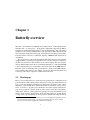
To start the control program TASCOM you have to type tascom in the commandline of an open terminal. The program starts up and if everything is right you should
view activity of the LED’s of the GPIB ethernet interface indicating that TASCOM is
trying to connect with the ECB module and the histogramming memory unit. After
Figure 1.1: TASCOM screen after start up.
start up it will display it’s version number, the current data file and the command file
directories plus a list of supported sub systems. It should claim support for the ECB
and MCA sub system as those are essential for operating the spectrometer. Don’t
worry about missing support messages for the temperature controller and the PREMA
voltmeter, these are devices being present at a particular synchrotron beamline in the
HASYLAB, DESY (Hamburg) and reveal the history of the control software as an
adapted4 version of the one that controls — or used to control — the horizontal liquid
surface diffractometer at BW1. It is worth mentioning that TASCOM provides the
command owl, that allows the user to easily communicate5 to external programs which
could virtually control anything and communicate back to TASCOM without the need
of a specific internal control software add-on or modification. The ODA on-line Data
Acquisition supports an external plotting software package, which comes particularly
handy for monitoring the current histogramming memory read-out of the PSD detector
signal. Then it will print the symbol table, multiplexer file, gearing and display file
4 After the transfer overseas from Leipzig to Pittsburgh the author of this manual upgraded the control
software TASCOM to the most recent version. Some adaptions for CMU are listed in a dedicated section in
this manual.
5 originally implemented by the author of this manual
1.2. TASCOM ROUND TRIP
3
names and locations, which are so important to the system that they deserve beeing
mentioned [3]. Finally it will print the TASCOM command-line prompt:
>_
You can type in TASCOM command sequences or execute macros which are inside the
command directory. The local command directory of the tascom account holds the
macros to operate the butterfly spectrometer inside the ˜/command/cmu/ folder.
1.2
TASCOM Round Trip
The control software of the butterfly reflectometer is the C-version of the program TASCOM6 that evolved from the original Fortran version developed at the danish national
laboratory RISØ in its glorious days. In the following a big picture view is outlined
in the hope to enable the user to grasp quickly the more detailed information from the
TASCOM user and extension manuals [2, 3] and even from its source code if needed.
The TASCOM program operations are centered internally around the values or
states of the so called symbol table that holds the user variable names, build in command names, timer and counter names, stepper motor names, their parameters settings
and their current position values. The source code and binary of TASCOM is located
in the cmu folder in the home directory of the tascomp account on the Linux work
station. Under normal user operation TASCOM updates its values in the
/home/tascomp/cmu/tas/symfil/symfil.bin
in an — unfortunately — binary representation. An ASCII representation of the symbol table exists but it is beeing used only in the rare case of a symbol table initialization
where TASCOM reads the ASCII symbol table and then creates a new binary symbol
table file. After such a procedure most likely information like current motor positions,
modified gear parameters, soft limits, user defined variables and so on are lost rendering the spectrometer in an ill defined state needing some work to be done to get all
symbol table values restored and return the spectrometer operational — at least from
the software side point of view. The ASCII source file being used in the CMU incarnation of the butterfly reflectometer is located at:
/home/tasfiles/symfil/cmu_sym.sor
on the tasfiles account. For the sake of completness the motor parameters, multiplexer and display files for the CMU butterfly installation are located in:
/home/tasfiles/command/cmu_gea.tas
/home/tasfiles/command/cmu_mux.tas
/home/tasfiles/command/cmu_dis.tas
Note the obvious adaptations of those files names to the particular installation and mind
to adapt your actions accordingly in case you want to follow procedures described in
6 TASCOM
is the shortcut for Triple Axis Spectrometer Communication program
4
CHAPTER 1. BUTTERFLY OVERVIEW
the TASCOM user manual [3]. TASCOM features its own macro language which is
somewhat fortranish in its syntax but does not require a strict format nor capital letters.
Macros can be defined and placed in the command directory in files with an extension
.tas in the file name. On typing a command in the command line TASCOM searches
first its symbol table and if that fails the command directory and if that failes TASCOM
issues an error message. In case you assign a value to a variable that is not yet defined in
the symbol table TASCOM adds a new variable to the binary symbol-table. Particularly
it created a new symbol in the symbol table if you accidently misspell a variable name.
In order to avoid a symbol table pollution you should delete accidently user created
symbols from the symbol table using the command dels, e.g. dels tempp [3].
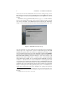
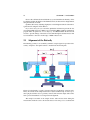
1
2
3
4
5
6
X-ray tube
PSD
Flight tube
Attenuator
Slit 1
Slit 2
7
8
9
10
11
12
Slit 3
sample table
Rotation arm source side rox
Rotation arm detector side rod
Height translation source arm tzx
Height translation detector arm tzd
13
14
15
16
17
18
Translation sample height tzs
Counter weight
Translation x-y sample txs, tys
Goniometer sample gxs, gys
Detektor holder
Göbel mirror
Figure 1.2: Butterfly scheme
1.2.1
Important motors
This is the list of the most important motor of the butterfly reflectometer. All the names
have been defined such in the cmu sym.sor.
tzs
tzx
tzd
translation z-direction sample-table
translation z-direction tower X-ray source-side
translation z-direction tower detector-side
1.2. TASCOM ROUND TRIP
5
rotation X-ray source-side arm
rotation detector-side arm
translation x-direction sample-table
translation y-direction sample-table
goniometer x-axis sample-table
goniometer y-axis sample-table
rox
rod
txs
tys
gxs
gys
Most of the motors are addressed in normal user operation indirectly by commands
through the execution of specific macros. Motors names not mentioned in this list are
the ones for the slits and absorbers. Those macros or cammands will be mentioned
later and the inspection of their source is encouraged.
1.2.2
Important system variables
In the original symbol table source variables– intended for a specific use – are defined
such as segn for the segment number suffix or fina for the prefix in the data file
names. Some system variables are state variables e.g. prsc, which sets the scaler
mode to either counting till a certain number — to be defined in another system variable
pres — of counts or time, others are read-only7 variables like timers and scalers, e.g.
I. A list of some of the more important system variables include:
I
TIM
RATE
PRSC
PRES
SEGN
DFIT
CEMA
MIDP
holds intensity value read by coun command
holds value of timer started by a coun command
set to 1 enables rate meter; set to 0 disables rate meter; i.e. continous counting
set scaler mode. If set to 0 scaler is in time mode; otherwise
i=1,2,3 selects number of counts from detector i. The butterfly
uses currently only one detector — the Braun PSD — which is
i=2.
holds the preset value for the scaler
holds current segment number
holds comment string for the current data file
center of mass calculated by built in statistic function in the
plot command
holds the mid point of internal statistics evaluation. Very useful
for scans.
You can print the value of a variable, a motor position or perform a calculation
using the print command ? f.x. the number of counts measured during the last coun
command:
?I
7 each symbol table entry has a scope field, a number that is used by TASCOM to discriminate the type
of a command sting after parsing it: variable, command, read-only variable, etc.
6
1.2.3
CHAPTER 1. BUTTERFLY OVERVIEW
Scans
Scanning the motor position against detector counts is a frequent task during operation
the butterfly. The basic scan macro sma for scanning the absolute position against
detector counts is provided in the tasfiles command directory. Its usage is
sma motor, start pos, end pos, steps, pres
The following line is frequently used for the sample height scan before a reflectivity
measurement:
?tzs sma tzs,tzs-0.3,tzs+.3,31,1
The first command ?tzs prints the current motor position, the second command
sma tzs... scans the motor tzs in 31 steps ±0.3 against its current position tzs.
Note that the value of the sample height is plotted before the height scan. This is a good
pratice in case you decide to move the motor position back to the original value. All
scans and macros can be stopped by hitting ctr-c. Mind that the sequence ctr-d
suspends on Unix/Linux a program to the background. If you happen to hit accidently
ctr-d instead of ctr-c TASCOM still keeps running in the background and you can
get the TASCOM console back to forground by typing fg into the terminal window.
After a succesfull scan you can assign the sample height to the calculated midpoint
value:
tzs=midp
The command directory of the butterfly reflectometer holds many more sophisticated
scan macros for operating the spectrometer.
1.2.4
Macros
The typical structure of a macro is explained in detail in the TASCOM user manual.
Nevertheless a particularity of the use of semicolons in TASCOM is beeing outlined
here. Whenever TASCOM parses a macro it parses the source till a the occurance of
a semicolon and then executes. This can have interesting consequences f.x. if you
decide to seperate operations in a macro by a semicolons and say the first piece till the
semicolon parses without an error message, then TASCOM will execute that part and
parse the next piece of code till the next semicolon. If a subsequent piece of code has
an error an error message will be issued and causes TASCOM to abort the execution
of the macro. It is thus adviced to check the macro for errors before executing it for a
scan, especially if that one is intended to take a long time.
1.3
Operation
In the following the normal operation of the butterfly reflectometer is outlined. We
assume the butterfly reflectomter is aligned, all sub-systems are up and running and
a liquid interface in the Langmuir-Blodgett trough of proper height is the sample. A
liquid surface has the advantage that it is horizontal by gravity, whereas a solid sample
1.3. OPERATION
7
might need first an alignment to be horizontally to the beam using the goniometer
motors, which is an obvious step preceding the following procedure.
1.3.1
Absorber
The detector should not get much more than 6000 counts/second. Thus the direct
beam must be attenuated in order to protect the detector (PSD), which is done by the
attenuator. The attenuator is modified slit where the motors moves instead of jaws
aluminium foils of different thickness into the direct beam. The four jars carry 2, 4, 8
or 16 layers of an aluminium foil, thus totally 16 absorber settings are possible. Make
sure that you select an appropriate absorber settings once you put the reflectometer into
a direct beam or low angle setting. attb number sets attenuator factor by selecting
a state between 0 and 15. State 15 has all absorber slides in beam and the highest
attenuation, state 0 all attenuation foils out of the beam. atten val set attenuator
value to an attenuation factor of at least val. For info from online help type help
’atten’. The macro atten defines internally attenuation factors for each of the
alumium absorbers, which go into the calculation od the attenuation factor atte.
atten_s0
atten_s1
atten_s2
atten_s3
=
=
=
=
2.4
4.8
27.2
777.8
!
!
!
!
-->
-->
-->
-->
M21
M14
M29
M13
-->
-->
-->
-->
ab0
ab1
ab2
ab3
These values should be checked. The macro patten prints the current absorber state.
1.3.2
Typical scan
A sample is prepared in the LB trough or a waver is mounted on a flat support in
the center of the sample table. The reflectomter is put in save starting state with the
command go home, which cares for slit settings of slit1, attenuator settings and sets
the reflectomter to 0.75 × αcritical so that the sample surface is expected to serve as a
mirror. The critical angle is stored in the user variable ac and it is up to the user to
update its value to e.g. water or silicon oxide surfaces ac h2o or ac si.
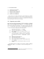
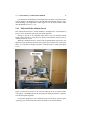
Figure 1.3: The flight tubes point to the sample placed in the center of the sample table.
A sample height scan is performed typically in the reflected position at butterfly setting
of the angle at 0.85 × αcritical .
8
CHAPTER 1. BUTTERFLY OVERVIEW
Open the shutter 1 on the front of the Siemens X-ray generator [1]. The reflectomter
is in a position where the sample serves (or should serve) as a mirror, and just the right
height of the sample has to be determined. This is usually done in a two step process.
In the first step select the motor tzs with the manual box and use the joy stick to move
the motor and watch the rate meter or the counts/second on the monitor from the ECB
module. Once you have found the maximum count rate you can start a scan.
>
>
>
>
attb
! or
bfly
?tzs
9
whatever the necessary attenuation is
0.85*ac
sma tzs,tzs-0.3,tzs+.3,31,1
If the scan is done and the result looks like a gaussian with a fwhm of ≈ 0.25 you can
set the sample height to the maximum.
> tzs=midp
In case you want to check alignment or make a scan of a waver you need to perform an
angular offset scan, which will be explained in more detail in the alignment section.
> soff -.3,.3,31,1
If a proper maximum is found, set the new angular offset value
> offbfly midp
in order to set the reflectometer to the maximum position. If the offset is off, repeat the
sample height and offset scans until you find iteratively a stable configuartion.
The command bfly al pha sets the incident and exit angle to the al pha. The
command sbfly abeg, aned, npoi, pres, i0 is the primitive scan macro for reflectivity scans. Its usage for complete scans be looked up in macros like gold.tas or
mucus.tas in the command file directory.
Slits
The slits are motorized and slit settings can be modified during operation. An example provide the scan macros mucus which calls macros like slitset1b to set the
horizontal opening of slit 1. The settings of slit2 and slit3 remain unchanged — as
set in the initial instrument alignment. The horizontal slit width/opening of slit 1 is
particularly crucial during an reflectivity experiment. For shallow angles of incidence
the horizontal width of slit 1 must be set small to reduce footprint size of the incoming
beam, whereas for larger angles of incidence the footprint of the incoming X-ray beam
has a reduced and it is desirable to make the horizontal width of slit 1 as wide as possible to get as many photons hitting the sample. Slit 1 and have horizonatl and vertical
openings whereas slit 3 has only a horizontal opening.
REFERENCES
9
Slit commands
Slit commandos operate on the current slit. The current slit is selected by the commands sel hsl [123] for a horizontal slit or sel vsl [12] for vertical apertures. The
slit help page provides additional information of the slit settings macros.
sel hsl [123]
sel vsl [12]
slpo
lcsl
mcslp p
mcslw w
scslp pmin, pmax, npoi, pres
scslw wbeg, wend, npoi, pres
rcslp p, w
select horizontal slit # to current slit
select vertical slit # to current slit
list all slit settings
list current slit setting
move current slit to pos
move current slit to width
scan relative to current position
scan slit width of current slit
rename current slit state to position and width
References
[1] Siemens. KRISTALLOFLEX 760 X-ray Generator, 1993–1995.
[2] Per Skaarup. TASCOM Extension Manual. Risø, 1997.
[3] Per Skaarup. TASCOM User Manual. Risø, 2003.
[4] Markus Weygand and John Zoll. Siemens Kristalloflex 760 Butterfly Reflectomter
(logbook). CMU, 2008.
10
CHAPTER 1. BUTTERFLY OVERVIEW
Chapter 2
Alignment
2.1
Coarse alignment
The coarse alignment is the optical adjustment of the detector and source arm. This
step is ususally necessary only after a complete dismantling of the reflectomter – rather
seldom.
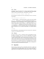
Figure 2.1: Butterfly, no parts mounted on the flight tubes.
The first step is to place the arms of the naked (figure 2.1) butterfly horizontal
as good as possible using the rotational degrees of freedom, i.e. motors rox, rod.
Make the motor adjustments from the manual box. Use first the scale of the goniomters,
there might be still some usefull marks from previous work. Then take the telescope
11
12
CHAPTER 2. ALIGNMENT
and use appropriate marks1 at the front and back end of the arm you want to level.
After leveling the arms place them on the same height using the translational degree of
freedom, i.e. tzx, tzd and the telescope. When this is done the to flight tubes have
to be aligned uniaxially. This is done by adjusting the lower arm 2tl in the plane of
incidence, so that both arms are aligned uniaxially. Use a horizontally levelled2 laser
to perform this task.
Obey laser saftey rules!
When you found an optical horizontal, remember (husk) this setting with the command:
> husk_hor
Later you can move the motors back to that horizontal reference position with the
command gohor. Help on alignment is availible in the TASCOM help system — just
type help ’refl’.
2.2
Adjustment of the Göbel mirror
The adjustment of the Göbel mirror falls into three stages.
1. search for the characteristic line (fx. after sealed vacuum tube exchange)
2. orient the beam along the flight tube axis
3. optimize the focused beam shape
Warning:
All work for Göbel mirror alignment must be done with X-ray tube
powered on and shutter open.
Follow radiation safety rules [4]
Use the portable counter before any new operation.
You must wear your radiation batches, especially the finger ring.
Use lead shielding against back scattered radiation.
The safest place is to behind the tube.
Stand only on side with mounting plate for the mirror and tube case.
Always close the shutter before you change a slit.
1 if you don’t find any good marks or scratches or whatever, go and take a ruler and scale and make your
own ones!
2 A laser can be levelled with the help of a tranparent hoase. Fill a 5m hoase with water and observe the
menisca of both ends.
2.2. ADJUSTMENT OF THE GÖBEL MIRROR
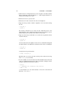
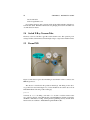
2.2.1
13
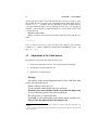
Adjustment of the Göbel mirror from scratch
Figure 2.2: The Göbel mirror and its skrews. Never touch the unlabeled ones.
slit 1
slit 2
illumination slit insert
exit aperture insert
a
b
c
d
e
f
moves the of Göbel mirror case against beam (focal height)
moves illumination slit (slit 1 ) against Göbel mirror
moves exit slit (slit 2 ) against Göbel mirror
tilts Göbel mirror against beam
tilts Göbel mirror against slits
combination of movement d and e of the Göbel mirror (better not move at all)
The adjustment of the Göbel mirror is done visually with the help of flourescence
screens and the X-ray eye, and CCD camera. The observation is done after the first
flight tube in the sample table areal. Remove all attenuator slides out of the beam (type
either atten 1 or attb 0). Insert the 6 mm slit in the slit 1 holder, remove the exit
slit (slit 2 (figure 2.2) and cover the opening of slit 2 at the side with a partially inserted
slit or a piece of led. Unmount slit 1 — from the butterfly scheme (figure 1.2) not the
Göbel mirror — if it is not yet unmounted and pose it on the floor or on the flat area of
the 2tu arm.
14
CHAPTER 2. ALIGNMENT
Operate the X-ray tube under lowest power (20 kV/5 mA) and open the shutter [2].
You must check for scattered radiation in the surroundings of the tube with the
portable counter and apply lead sheets and lead plastic shield as needed. Never
stand at the side where the slits are being inserted in the Göbel mirror case, when
the shutter is open (the front side in figure 2.2).
The mirror is essentially a plate that must be lowered and slightly tilted against the
incoming X-ray beam. The correct tilt is required to get the desired monochromatic
X-ray beam.
First level the skrews d, e and f so that they align flatly with the case. You must
always move the skrews first in downwards direction and then upwards to the desired
position in order to compensate for the mechanic backlash. You should be able to see
a simple bright band on the flourescent sreen above the center of the flight tube (figure
2.4 i). Make sure that this band is not confined by the illumination slit and use the
skrew b for adjustment. Turn skrew a and move the band until an upper confinement
appears. Now tilt the Göbel mirror by turning skrew d up to the point where the upper
confinement remains unchanged (figure 2.4 ii). The mirror is positioned parallel to the
beam.
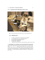
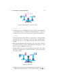
Figure 2.3: The major steps in the Göbel mirror alignment. i) with illumination slit
6 mm a broad bright band is visible on the flourescent screen or the X-ray eye. ii) tilt
Göbel mirror parallel to the X-ray beam. iii) insert the 1 mm illumination slit and select
the CuKα line. iv) insert the 0.6 mm exit slit.
The next step is to tilt the mirror forward, by turning skrew d inwards into the
casing. At some point the Kβ line will appear and then the Kα line3 The tilt (skrews d,
e) must optimized so that the Kα line gets intense.
3 The
Kα line is made of two lines Kα1 , Kα2 that are close together.
2.2. ADJUSTMENT OF THE GÖBEL MIRROR
15
Now insert the 1 mm illumination slit and place the 6 mm in the exit aperture holder.
Vary the height of the illumination slit (skrew b) until the bright line reappears and a
small remaining of the bright band is visible (figure 2.4 iii). If only the band is visible
then the illumination slit is too low.
2.2.2
Shift and tilt the collimated beam
The collimated beam must be oriented uniaxially to the flight tubes. A small deviation
however can be dealt with easily in the subsequent alignment.
Changes in the tilt of the collimated beam must be done by altering the initial
height of the Göbel mirror casing (skrew a). Then proceed with the same procedure as
described in the last section.
When the colliminated beam is oriented well enough uniaxially respectively to the
flight tube, insert the 0.6 mm slit in the exit aperture (slit 2 in figure 2.2) of the Göbel
mirror case and adjust its height using skrew c until the beam is visible again (figure
2.4 iv).
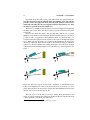
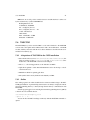
Figure 2.4: The detector holder can be used for holding the X-ray eye with an cylidricatal adapter or the PSD right after the first flight tube during Göbel mirror optimazation and subsequent alignment.
For the final optimazation of the collimated beam power the X-ray generator up the
operating power of 45 kV/35 mA and wait least 90 min to reach termal stabilty.
16
CHAPTER 2. ALIGNMENT
Observe the collimated beam with the X-ray eye and maximize the intensity of line
by adjusting slightly the height of the illumination slit, the Göbel mirror height and tilt
using the skrews b, a and d.
Optimize the beam by adjusting slightly the exit slit height and the tilt of the mirror
against the slits using the skrews d and c.
If you don’t trust your eyes and want quantitative information perform the last
step with the PSD and observe MCA read out with the online graphical visualazation
program under an update rate of 1 second [1, 3]. You must attenuate the direct beam
in order to prevent damage of the detector. Start with the highest attenuation factor and
lower it until the count rate is in the range of 6000 counts/second.
2.3
Alignment of the Butterfly
The butterfly geometry is an essentially symmetric setup designed for specular reflectometry on liquid or other planar surfaces oriented in the horizontal plane.
Figure 2.5: The lengths len1 and len3 must be known for reflectivity operation mode.
The xy movements of the sample table must be adjusted with the help of a telescope so
that a pin placed in the recess is perfectly centered. The centered sample table carries
later a precision machined cross being used in th alignment.
The sample is mounted on the sample elevator table and rests there during the
measurement. Both the source side and the detector side arm possess a translational
2.3. ALIGNMENT OF THE BUTTERFLY
17
and a rotational degrees of freedom (and even more degrees of freedom if we consider
the possible slit movements). Due to the pattern of the arm movements in an experiment
people called this type of reflectometer a butterfly. The initial optical alignmet of the
flight tubes into a horizontal plane serves as the starting point for the fine alignment
of the butterfly (pp. 11). The fine alignment breaks up into the following steps (these
steps serve as a guidline and don’t replace (totally) own thinking; scan ranges needed
may be different and so on; it is also strongly recommended to look into the macros.):
• Mount the aluminium plate with the round recess in the center on sample table.
You might have to unmount another aluminium plate from the sample table tower
— most likely the ground plate for the Langmuir Blodgett trough.
• Center a pin on the sample table (take the small goniometer with the sharp pin
which fits precisely in the round recess of the square aluminium support plate).
You the telescope as a visual aid and observe the tip under a 90◦ rotation of
the sample table (to do this unhinge the gear box of motor TS. Perform these
rotations manually and be gentle with the cables around.)
• Determine len1 and len2 with steel rulers as well as you can.
• Mount the detector holder on the second flight tube so that it can carry the PSD
in the sample table area. Search the direct beam moving the height of the second
flight tube (tzd) using the manual box.
• Mount slit 1 and align slit 1. Set the attenuator and start with the hightest at-
Figure 2.6: Align slit1 with the PSD mounted in the sample tabe area.
tenuation factor (attb 15 or atten 200000). The unit of the slit motors
movements are set to multiples of 100 µm. Most likely the the slit settings from
the previous alignment are somewhat useful, especially the widths and position.
Select the horizontal aperture of slit1 and open it 500 µm wide.
> sel_hsl 1
> mcslw 5
The next step is to perform a height scan of the slit aperture. The macro scslp
performs a scan relative to the current position and returns to the position before
the scan, e.g.
18
CHAPTER 2. ALIGNMENT
> scslp -30,30,31,1
Mind that these scans should be used with some care so that you don’t exceed
the mechanical limits in the planned jaw movements. Reduce the scan range
from ±30 (as in the example above) to say ±10 for the fine scan. Move the slit
position to the center of the scan.
> mcslp midp
After the slit height is found, check for the slit width and scan the slit width using
the current slit width scan:
> scslw 70,-10,81,1
Like in the position scan this macro returns to the slit state before the scan.
You can assign a slit state a position value p or/and the slit width w. The command macro uses internally the remo command [3]. You are responsible for a
meaningful result.
> rcslp p,w
And finally you can print the current slit settings/values.
> lcsl
For the sake of completness the macro slpo prints info about all slits.
• Mount the X-ray eye instead of the PSD in the detector holder using the custom
machined cylindrical aluminium adapter observe the direct beam with the X-ray
eye.
• Place the cross in the sample table center and move the sample height table
tzs so that the cross just obscures the direct beam (use the Manual box, slow
movements). Note its position value into the TASOM variable tzsb.
• Track the length len1. The command bfly al pha moves the butterfly into the
expected position for specular reflectivity under the angle of incidence al pha.
The proper operation depends on correct values for the lengths, len1 and len3 in
TASCOM. The read the current values in TASCOM type
> ?len1,len3
Assign your newly measured length values to the TASCOM variables len1 and
len2 and make TASCOM remember the current position of the X-ray side of the
butterfly as its reference horizontal position for reflectometry calculations.
> husk_xwing 0
2.3. ALIGNMENT OF THE BUTTERFLY
19
Figure 2.7: Track length len1 with the cross and X-ray eye.
If len1 was perfectly correct, the direct beam would always hit the center of the
cross and being obscured from the X-ray eye (check tzs with manual box) if
the incoming arm is being set to the calculated position for any chosen incoming
angle al pha. The macro which moves only the motors for the first arm into the
calculated butterfly position under an angle al pha is called xwing and used like
> xwing 2
in order to position the first arm to the theoretical position for the angle of incidence of 2◦ . The tracking of the error is done by observing the deviation of the
center of the cross from the beam under various angles, like 0, 0.5, 1, 1.5, 2, 2.5,
3, 3.5, 4, 4.5 degrees. Obviously the height of the X-ray eye must be adjusted
for larger angles of incidence. The theoretical relative height displacement of
the flight tube respective to the horizontal position for an angle of incidence α is
txhe = len1 ∗ tan α. Note down the observed deviation ∆z = tzs − tzsb, where tzs
is the position of the sample height where the cross precisely obscures the X-ray
beam. The macro diffs prints this difference for convenience (that is the reason you stored the sample height for the horizontal case). Make a file with the
values α for the angles of incidence and the observed deviations ∆z. You can use
gnuplot to fit the linear regression curve (type help fit inside gnuplot). Fix
the value of len1 if a systematic deviation could be traced.
20
CHAPTER 2. ALIGNMENT
• Unmount detector and align the detector arm to the plane of incidence with the
help of a flourescent screen and adjust the 2tl, either using the manual box or
manually with unhinged motor gears.
• Mount slit2 and slit3, open jaws wide
• Mount detector holder towards the end of the second flight tube.
• Align slit2. The procedure is similar to alignment of slit1. Start with selecting
the slit2.
> sel_hsl 1
> mcslw 10
The scanning commands are now exactly the same. Mind that because of the
slight divergence of the collimated beam the slit must be set wider in order to
catch the direct beam. Scan the position and the scan the width.
• Align slit3. The same procedure like for slit1 and slit2 except that this slit has
only horizontal jaws.
> sel_hsl 3
> mcslw 15
Close the vertical jaws slit1 slightly in order to allow to discriminate background
and signal channels on the PSD. The commands needed could be something like
> sel_vsl 1
> mcslw 12
A sample slit scan is performed, like:
> scslp -25,25,31,1
Remember that you can move the (here vertical) position with the slit moving
macro mcslp p if you need that.
• In order to track len3 follow the direct beam with the PSD mounted at the back
of the second flight tube under various angles of incidence, starting by remembering the optical horizontal reference position
> direct 0
> ! rememeber the reference TZD position
> sdhe = tzd
to set the instrumet to 0 ◦ tilt. Set the butterfly to various tilts of the dirct beam
like 0, 0.5, 1, 1.5, 2, 2.5, 3. . .
2.3. ALIGNMENT OF THE BUTTERFLY
21
Figure 2.8: The butterly set to the direct beam.
> direct 0.5
Scan the height of the second flight tube, note the found mid p and its difference
to the theoretical value sdhe, which was calculated by the direct macro. A
convenience macro exists in the command directory that prints that difference.
> diffd
Write down the angles and the differences on paper and/or to a file and calculate
the linear regression f.x. with gnuplot. In case you spot a systematic deviation correct the value of len3 accordingly and check if the correction was done
properly.
• Mount Langmuir Blodget Trough and prepare a bare water surface. Place the
glass block in the range of the foot print and fill the trough with water, so that
the are cobered by a 300µm water layer above.
• Find the angular offset of the beam regarding the water surface. The optical
horizontal is a straight line by construction, which may or may not be perfectly
horizontally oriented.
Figure 2.9: Offset scan.
Remember that horizontal state for TASCOM with the command husk bfly
0. Then make a sample height scan — the arms still horizontal — and position
22
CHAPTER 2. ALIGNMENT
tzs where the sample cuts half of the beam. Then set the butterfly into specular
reflective position and scan the sample height again and set tzs to the mid p.
> bfly 0.85*ac
> ?tzs sma tzs,tzs-0.3,tzs+.3,31,1
> tzs=midp
Then scan the angular offset and place the offset to the mid p.
> soff -.3,.3,31,1
> offbfly midp
You must probably repeat the sample height and offset scans and get iteratively
to the desired state. Once you have found a proper alignment remember this state
for TASCOM as the reference state.
> husk_bfly 0.85*ac
• Make a reflectivity scan of the bare water surface and check for the critical angle.
You can start as simple as
> slitset1b
> attenb 8
> sbfly .1*ac,2.5*ac,22,3000,1
Adapt old scan macros if necessary, especially for slit settings and channel number for signal and background of the PSD.
References
[1] MBraun. Mbraun 50mm PSD, Manual – now HECUS.
[2] Siemens. KRISTALLOFLEX 760 X-ray Generator, 1993–1995.
[3] Per Skaarup. TASCOM User Manual. Risø, 2003.
[4] Markus Weygand and John Zoll. Siemens Kristalloflex 760 Butterfly Reflectomter
(logbook). CMU, 2008.
23
24
CHAPTER 3. MACROS
Chapter 3
Macros
3.1
TASCOM
go home
bfly al f a
sbfly abeg, aend, npoi, pres, i0
soff o f f a, o f f b, npoi, pres
offbfly o f f
husk bfly atru
set the butterfly in a safe starting position.
move butterfly to specular reflectivity position of angle of
incidence al f a.
basic reflectivity scan
offset angle scan for current specular reflectivity position.
Typically 0.85 × αcritical .
apply an angular offset to current butterfly/alfa state.
remembers (danish at huske) the current butterfly state as
the state for specular reflectivity of an angle of incidence
atru. This is achieved by determing offset values, which
are added to the theoretical positions for motor movements (elevator towers translations and rotations of the
flight tubes). The command freezes the current state as
the reference for the angle atru.
lisa
set the butterfly to direct beam of angle al f a
set only the X-ray source arm to the butterfly angle al f a
set only the detector arm to the butterfly angle al f a
like bfly but only prints hypothetical movements. No
movements made.
like direct but only prints hypothetical movements.
No movements made.
list current butterfly state
sel hsl num
sel vsl num
lcsl
slpo
mcslp p
mcslp w
rcsk pos, width
sabs abn, abst
select horizontal slit num, num ∈ 1, 2, 3 as the current one.
select vertical slit num, num ∈ 1, 2 as the current one.
list curren slit positions.
list all slit positions.
move current slit position to p.
move current slit width to w.
remo current slit setting to pos and width.
moves absorber blade abn in if abst = 1, or out if abst = 0
lpsd
read contiously the MCA histogramming memory. This
macro is useful for observing the current PSD counts.
direct al f a
xwing al f a
dwing al f a
bfly pri al f a
direct pri al f a
3.2. GNUPLOT
3.2
25
Gnuplot
Macros can be loaded in gnuplot by the command load ’macro’. A useful macro
is frsn which has Fresnel functions for the reciprocal and angular space defined.
set log y
qc_h2o=0.0217
qc_si=0.0314
qc=qc_h2o
ff(x)= (x*x-qc*qc)**.5
f(x)= x < qc ? 1 : ((x-ff(x))/(x+ff(x)))**2
fs(x,s)= f(x)*exp(-x*x*s*s)
a2q(x)=4*pi/1.542*sin(x*pi/180.)
fa(x)=f(a2q(x))
fsa(x,s)=fs(a2q(x),s)
The macro reload repeats the last plot commando, which comes handy during
scans. Printer output can be placed conviently into a macro such as print. Adapt
it to the latest printer names and/or the desired Postscript (or other terminal options)
options.
set ter post color
#set output "|lpr -Pbutterfly"
#set ter post color
set output "|lpr -Phpcolor"
#set ter post mono
#set output "|lpr -Posage"
repl
set output "plot.ps"
repl
set ter X11
repl
Rich documentation for gnuplot is available inside the program through the built in
help system and the gnuplot home page http://www.gnuplot.info/.
3.3
Perl
The macro tasrd extracts information from TASCOM data and array files. Extract
for example the data columns for Q1, REFL, SREFL from a reflectivity data file
xxxx007.ref with
tasrd -s "Q1 REFL SREFL" xxxx007.dat
Values stored in the paramter line are being extracted with the additional option
switch -p, e.g. tasrd -p -s "ss se bs be" xxxx007.ref. Arrays are
accessed by indicating square brackets, or by an index range
26
CHAPTER 3. MACROS
tasrd -s "Q1 DD[]" xxxx007.dat
tasrd -s "Q1 DD[23:90]" xxxx007.dat
The sum over an array range is taken with prefix s inside the square bracket after
the array name, e.g
tasrd -s "Q1 DD[s23:90] DD[s100:200]" xxxx007.dat
Values stored in the paramter line are extracted just with the additional option
switch, e.g. tasrd -p -s "ss se bs be" xxxx007.ref.
A mixed access to file parameter and header parameter is possible as well (in that
order) with the option -P, e.g.
tasrd -s "Q1 REFL SREFL" -P -s "ss se" xxxx007.ref
Type tasrd -h for the build in help.
3.4
R
R is a software environment for statistics with rich graphical capabilities and features
a functional programming language. In some ways it is similar to Matlab or IDL.
An introduction is available in the documentation at the home page of the R-Project
http://www.r-project.org/ or closer to you at http://lib.stat.cmu.edu/R/CRAN/. A reference card is located at http://cran.r-project.org/doc/contrib/Short-refcard.pdf.
Type R in a free terminal to start R. The command source("parratt.R")
reads the file parratt.R into R. This command is used for running batch files or
loading macros.
3.4.1
Reflectivity Calculation
The Parratt iteration is implemented in the parratt function.
function(x,d,del,sig=2.7,bet=0) {
theta <- 0.5*abs(x);
nmax <- length(d);
nx
<- length(x);
rn <- an <- f <- array(0i, c(nmax,nx));
if (length(sig) == 1) {
sig <- rep(sig,nmax);
}
if (length(bet) == 1) {
bet <- rep(bet,nmax);
}
3.4. R
27
for(i in 1:nmax) {
f[i,]=sqrt(thetaˆ2-2*del[i]-2i*bet[i]);
}
an[1:(nmax-1),] <- (f[1:(nmax-1),]-f[2:nmax,])/
(f[1:(nmax-1),]+f[2:nmax,]);
# modified reflection coefficient
if (length(sig) == length(d)){
msig <- array(sig[2:nmax]ˆ2, c(nmax-1,nx));
an[1:nmax-1,] <- an[1:(nmax-1),]*
exp(-2*msig*f[2:nmax,]*f[1:(nmax-1),]);
}
for (n in nmax:2) {
rn[n-1, ] <- exp((2.*d[n-1]*-1i*f[n-1, ]))*
(rn[n, ]+an[n-1, ])/(rn[n, ]*an[n-1, ]+1.);
}
Re(rn[1, ]*Conj(rn[1, ]));
#r <- Re(rn[1, ]*Conj(rn[1, ]));
#r;
}
As an example of its usage a Fresnel curve for neutrons is being calculated. The
function qc2nrho calculates the neutron scattering length density from a given critical
angle.
qz <- seq(0.001,0.25,by=0.005)
qc=0.021764
qc2nrho(qc) -> rsub
slux <- 2.817938e-05 # X-rays
slun <-1 # Neutrons
slu = slun # the example is for neutrons
parratt(qz, c(0,0), 2*slu*pi*c(0,rsub),sig=2.7) -> refl
plot(qz, refl, log="y")
3.4.2
Read Data Files into R
The following example illustrates how tasrd macro is being used to read some reflectivity data file ndata.ref into R.
rdng7 <- function(file="pgmD2O_0507.ref",
path=/home/tascom/data/) {
# read corrected Neutron data files
28
CHAPTER 3. MACROS
parameter=’"Qz R dR"’
cur_file=paste(path,file,sep="")
command=paste(’tasrd -R -s’,parameter,cur_file);
print(command);
data = read.table(pipe(command), header=TRUE);
return (data)
}
mypath="/home/tascom/myneudata"
myfile="ndata.ref"
data=rdng7(file=myfile,path=mypath)
# print data structure information
str(data)
Note particularly the lines with the paste command that glues several strings
together to one command string. The convenience function num2fnum(segn) adds
leading zeros to numbersand formates them in the same way TASCOM does the segn
suffix in the .dat file names. This command (the perl macro tasrd. . . ) is then
exectuted in the read.table(pipe(), ) command.
3.4.3
Tweak Reflectivity Data
A typical reflectivity scan on the butterfly is made of several scans with different slit
and attenuator settings. Overlaps of subsequent scan serve to determine the overlap
factor which comprises slit and attenuator settings and possibly sample artefacts.
husk_ac=ac
ac=ac_h2o
slitset05
attenb 7
sbfly 0.1*ac, 1.5*ac, 31, 3000, 1
attenb 3
sbfly 1.3*ac, 3*ac, 25, 3000, 1
attenb 0
sbfly 2.7*ac, 4*ac, 15, 3000, 1
slitset1b
sbfly 3.7*ac, 5.5*ac, 15, 3000, 1
slitset3
3.4. R
29
sbfly 4.5*ac, 15*ac, 10, 3000, 1
slitset5c
sbfly 13.5*ac, 28*ac, 14 , 3000, 1
sbfly 29.0*ac, 5.1, 3, 3000, 1
!
date
attenb 8 slitset1b
ac=husk_ac
The whole reflectivity scan comprises seven pieces and only the last two ones have
the identical slit and attenuator settings. The slitsetXX macros contain setting for
the slit 1, the footprint slit.
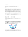
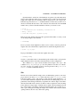
Figure 3.1: The slit width on the left defines the width of the incoming beam under
angle α. The wider the beam is the larger the footprint f gets; f = w × sin α. The
divergence of the beam is dominated by the Göbel mirror divergence (≈ 0.05◦ ).
slitset05.tas:
! small angle
sel_hsl 1 mcslw 0.5
sel_hsl 2 mcslw 7
sel_hsl 3 mcslw 8
sel_vsl 1 mcslw 12
ss=115 se=225 bs=10 be=110
iv=1
?ss,se,bs,be
slitset1b.tas:
! small angle
sel_hsl 1 mcslw 1
sel_vsl 1 mcslw 12
sel_hsl 2 mcslw 7
sel_hsl 3 mcslw 8
!ss=120 se=220 bs=10 be=110
ss=115 se=225 bs=10 be=110
30
CHAPTER 3. MACROS
iv=1
?ss,se,bs,be
slitset3.tas:
! medium angle
sel_hsl 1 mcslw 3
sel_vsl 1 mcslw 12
sel_hsl 2 mcslw 7
sel_hsl 3 mcslw 8
! slitset3/slitset1b
2.98864
iv=1
ss=115 se=225 bs=10 be=110
slitset5.tas:
! slit combination
sel_hsl 1 mcslw 5
sel_vsl 1 mcslw 12
sel_hsl 2 mcslw 12
sel_hsl 3 mcslw 14
iv=23.30606
! iv=39.89384
bs=20
be=110
ss=120
se=220
?ss,se,bs,be
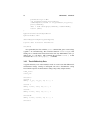
Use the function rdbfly to read reflectivity data of this type of scan. Assuming
the current data path is /home/tascom/data/cmu2009/mark/, the prefix fina
is called mark and the scan starts with the segn 123, the data are being read with
following command.
cur_path="/home/tascom/data/cmu2009/mark/"
dat=rdbfly(segn=123,fin_segn=-1,fina="mark",path=cur_path)
Assuming the overlap factors have been determined somewhere else (f.x. in gnuplot) and stored in R in the array mm the reflectivity data are plotted is plotted with the
command
mm =c(3000.000, 30.000, 12.000, 2.500, 2.000, 1.475)
plrty (dat, facs=calc_facs(mm) )
# obviously the overlap factors can be adjusted
# in a straight forward manner by changing values in mm
The next step is to discriminate the signal channel form the background ones. At
low momentum transfers qz or at small angles of incidence α for that matter the signal
to noise ratio is so high that we may neglegt the background. Since the vertical aperture
is not changed during the reflectivity measurement we can use the small angle region
for the signal/background discrimantion.
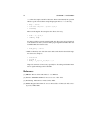
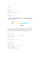
The plrty command displays per default the 2D image (figure 3.2) of the reflectivity scan, where on the y-axis the PSD channels are being displayed (up to the applied
overlap factors) and on the x-axis the momentum transfer qz . R provides the function
31
50
100
1:256
150
200
250
3.4. R
0.1
0.2
0.3
0.4
0.5
0.6
0.7
dat$QZ[sndx$ix]
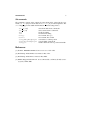
Figure 3.2: The 2D image of a reflectivity scan of a water surface in the Langmuir Trough displayed using the command plrty. With the build in R command
locator() it is easy to determine the channels numbers in the image with the mouse.
locator()1 that gives you coordinates of the image back you have clicked at. Click
with the left mouse button the on the borders of the signal range and do use many spots
in the low angle region and determine the signal range ss:se (signal start : signal
end). Determine the backgr ound range bs:be. Don’t use blindly a too low channel
number for bs in order to avoid the detector edges. Update the slitsetXX macros
to the new ranges.
The reflectivity data is being recalculated based on the novel ranges with the twrty
function.
twrty(dat, facs=calc_facs(mm),
bounds=list(ss=126,se=216,bs=15,be=125)) -> ref
Finally the data structure ref can be inspected with the R command str. An easy
way to store the corrected reflectivity data is using the R command write.table.
str(ref) # shows data structure
write.table(ref,"H2O.ref",row.names=FALSE,quote=FALSE)
1 type
help(locator) in R for build in help
32
CHAPTER 3. MACROS
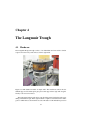
Chapter 4
The Langmuir Trough
4.1
Hardware
The Langmuir Blodgett Trough consists of an aluminium enclosure with a window
capton foil for the X-rays and carries a teflon trough inside.
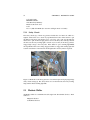
Figure 4.1: Film balance mounted on sample table. The small insert schows the aluminium support rails and the plexi glass pieces that support the trough. The trough is
fixed by four screws from below.
The temperature in the trough can be controlled using water flowing through copper
tubings beneath the trough. The trough mechanics comprises an electrical motor with a
gear box which drives a teflon barrier via a belt. The author of this manual has precision
33
34
CHAPTER 4. THE LANGMUIR TROUGH
machined a barrier made of Delrin.
Sensors can be accessed from outside the casing via air tight plugs such as the
barrier position read out (a potentiometer), a Pt100 temperature sensor, oxygen sensor
and the Wilhelmi sensor for surface tension measurements.
4.2
Tiger
The hardware is controlled by a Film Balance Controller designed by Bernd Kohlstrunk
at the University of Leipzig. The controller can command the film balance stand alone.
For data read out however some external computer must communicate with that controller via the serial interface. The film balance controller comes with its own documentation [1, 2].
4.2.1
Isowiso
XF A program written by the author of this manual — Markus Weygand — can issue
commands to and read data from the film balance controller. It is made available in the
local /̃bin directory of the tascom account. The communication is done with serial
protocol over an USB to serial interface converter. In order to read the current status
(i.e. position, lateral surface pressure and area) from the film balance controller type
isowiso -a
or
isowiso -l 1
for a continous output every second.
Examples of isowiso usage are:
isowiso -v -a
read current status i.e. position, lateral surface pressure
and area.
isowiso -v -l arg
read current status every arg second.
isowiso -v -b
read current barrier position
isowiso -v -l arg
read current status every arg second.
isowiso -T
switch sets output prope for TASCOM command the
owl.
isowiso -b arg
set barrier position soll
isowiso -p arg
set lateral surface pressure soll
isowiso -s arg
set speed index (0..9)
isowiso -v -g 1 -f xxx.ref store curent status to file xxx.ref every second
isowiso -c ”a comment”
add this option to the above command to store a comment
in the created data file.
Read the current status from inside TASCOM with the command
owl ’isowiso -T -a’,pos,pi_lat,area
REFERENCES
35
which stores the result of to the TASCOM user variables pos, pi lat and area.
Type isowiso -h for the build in help information.
References
[1] Bernd Kohlstrunk. Manual: Balance Controller Version 2.0. University of Leipzig.
[2] Bernd Kohlstrunk. Menu scheme Balance Controller. University of Leipzig.
36
CHAPTER 4. THE LANGMUIR TROUGH
Chapter 5
Technical Notes
Finally a collection of facts and pieces of useful information on the equipment are
given.
5.1
JJXray
This company did design and construct the spectrometer. They are located in Danmark.
Their web page is http://www.jjxray.dk/conus.html.
JJ X-ray A/S
Diplomvej 377, Scion-DTU
DK-2800 Kgs. Lyngby
Danmark
5.2
Telephone:
Fax:
+45 4776 3000
+45 4776 3001
VAT:
DK-2952 3215
Siemes Kristalloflex 760 X-Ray Generator
The Kristalloflex is the high voltage source for the sealed X-ray vacuum tube. This
device is usually part of a Siemens1 X-ray solution. JJ-Xray chose only the generator
part for the butterfly design. Siemens no longer owns the X-ray department and sold it
to Bruker. Contact Bruker AXS for Inc for service needs.
1 It
is helpful to tell that to a Bruker AXS service person.
37
38
CHAPTER 5. TECHNICAL NOTES
USA and Canada
BRUKER AXS Inc.
5465 East Cheryl Parkway
Madison, WI 53711-5373
USA
Tel. +1 (800) 234-XRAY (For customers calling from US or Canada)
5.2.1
Safety Circuit
The safety circuits [3] of the X-ray generator include the door interlook, which is a
mgnetic switch at the door to the X-ray experimental enclosure. If this circuit is open
the shutter at the X-ray tube holder closes or does not open. One way interrupt the
interlock is to pull off the bana plug at the bottom of the X-ray tube stand [6]. Outside
the enclosure an X-ray warning light is switch on (via a relais), if the X-ray generator
engages high voltage to the X-ray tube. If the shutter is open a warning light inside
the experimantal enclosure is being engaged. Failure to engage this warning light will
result in a breakdown of the interlock. If the light bulb is dead ity must be replaced.
Figure 5.1: Backside of the X-ray generator. Customized 9 pin and 13 pin plugs bridge
safety circuit settings [3]. The safety cables serve for the interlock, the X-ray warning
lamp and the shutter warning light bulb.
5.3
Haskris Chiller
the Haskris chiller is a refurbished model bought from JS Technical Services. Their
address is
Marguerite Stauver
JS Technical Services
5.3. HASKRIS CHILLER
39
(940) 382-2934 Voice
(940) 898-0150 Fax
6159 Moss Rose Lane
Aubrey, TX 76227
www.jstechnicalservices.com
e-mail: [email protected]
However since it is a Haskris device, you better deal with Haskris for spare parts,
such as the brass pump.
Figure 5.2: Haskris chiller. The brass pump is a consumable.
Hi Marcus,
PN 1370, Pump Model 102L100F11XX, $131.91 ea., excluding freight.
Pump includes new coupling.
Doug Wagner
Haskris Co.
tel 847-956-6420, x243
40
CHAPTER 5. TECHNICAL NOTES
fax 847-956-6595
email: [email protected]
If you change the X-ray tube you must switch off the chiller and unhook the hoases
from the tube stand. Remember which tube was pumping the water in and which one
out. The direction matters.
5.4
Sealed X-Ray Vacuum Tube
The X-ray source is a fine line copper Kα sealed vacuum source. The operation power
settings are 45kV, 35mA. Increase first the high voltage to target value and then current.
5.5
Braun PSD
Figure 5.3: The detector gaz bottle. The fitting is customized in order to connect to the
MBraun gaz hoases.
The detector is described in the producers manual [2]. The fitting for the detector gaz has been customized (figure 5.3). Select the PSD as the current detecor from
TASCOM with the following counter setting [5]
prsc=2
You must set rate to 0 during a scan and to 1 to be able to read the current counte
rate on the b/w display of the ECB module. The TASOM user manual [5] describes
the MCA commands for reading, clearing the histogramming memory and the timer
functions that are availible to TASCOM through the ECB module.
5.6. TASCOM
41
MBraun no more sells position sensitive detectors and this business is taken over
by the austrian X-ray systems GmbH HECUS.
Reininghausstrasse 13a
A-8020 Graz, AUSTRIA
Tel. +43 (0)316 / 48 11 18
Fax: +43(0)316/48 11 18 − −20
e-mail: officehecus.at
Office Hours:
Mon – Thu 08:00 – 16:00h
Fri 08:00 – 12:00h CET
5.6
TASCOM
The TASCOM [4, 5] version used in CMU is v3.15 and is identical to the TASCOM
version used at the liquid surface diffractomter with some modifications. The ECB
module, ancillary electronics and the motor drivers hardware is described in the documentation from JJX-ray [1].
5.6.1
Adaptations of TASCOM for the CMU installation
• Moved home directory from /usr/users/tascom to /home/tascom, similarly moved the accounts /home/tascomp and /home/tasfiles. Some
header files of the TASCOM source have been changed.
• The mca.c file is being patched to work with the local MCA.
• Gpib driver updated to stable National Instrument version hooked up to a dedicated network card.
• Makefile modified for updated gpib driver.
• The symbol table is newly defined for the butterfly at CMU.
5.6.2
Online
The online program is an online visualization for current scan that belongs to the TASCOM [5] distribution. A particular important feature is its ability to display the current
mca histogramming memory content (through shared memory communication with
TASCOM).
Start the program pgplot for monitoring the current histogramming memory (MCA)
content from a free terminal window.
cd /home/tascom/tasplot_Dec03
./plot 3 0 0 3 0
You can monitor the MCA readings continously with the TASCOM command sequence
42
CHAPTER 5. TECHNICAL NOTES
> whle 1..eq.1 cmca wait 1 rmca next
This sequence is for convenience stored in the macro lpsd in the command directory.
References
[1] Jens Linderholm. Løsche Leipzig, S2641a. JJ X-Ray, 1996.
[2] MBraun. Mbraun 50mm PSD, Manual – now HECUS.
[3] Siemens. KRISTALLOFLEX 760 X-ray Generator, 1993–1995.
[4] Per Skaarup. TASCOM Extension Manual. Risø, 1997.
[5] Per Skaarup. TASCOM User Manual. Risø, 2003.
[6] Markus Weygand and John Zoll. Siemens Kristalloflex 760 Butterfly Reflectomter
(logbook). CMU, 2008.