1
PaleoMagnatics Lab Cookbook
Introduction
Welcome to the P-Mag cookbook. This is a compilation of instructions on how to run the
various instruments in the P-Mag lab aboard the JOIDES Resolution. This manual has been
compiled from instrument manuals, cookbooks, documents and files from former techs, end of
leg tech reports and a lot of verbal and email input from assorted present and former techs. The
goal of this cookbook is not to replace the equipment manuals, you will still probably need to
refer to them if you have problems. We simply hope to supplement those manuals with the
knowledge picked up by the techs over many years, all those little tricks of the trade that make
life so much easier. Considering that the P-Mag lab is a strange mix of the state of the art and
the almost obsolete instrument, these little tricks often form the thin line between a smoothly
functioning lab and a very expensive disaster. In addition, where no manuals exist, hopefully we
have included explicit enough instructions to get you by. Please review this cookbook at least
once a year.
Table of Contents
Page:
Super-conducting Rock Magnetometer - Model 760 (Cryo-Mag), 2G Enterprises
CHAMP (Tensor Tool), Tensor Inc.
Impulse Magnetizer - Model IM-10, ASC Scientific
Minispin Magnetometer - Molspin, Ltd
Demagnetizer - D-2000 A/F, D-Tech Precision Instruments
Magnetic Susceptibility Meter - Kappabridge KLY-2, Geofyzika Brno
Thermal Specimen Demagnetizer - TSD-1, Schonstedt Instrument Company
Archive Multi-sensor Track (AMST) --- See Corelab
-
Magnetic Susceptibility Meter - MS2F, Bartington
-
Spectrophotometer - CM 2002, Minolta
Digital Imaging System (DIS), Geotek --- See Corelab
Cookbook – PMAG
1
Super-conducting Rock Magnetometer-Model 760
Cryogenic Magnetometer (Cryo-Mag),
Vendor:
Software:
Vendor Manuals:
2G Enterprises
Long Core, version 3.0, Leg 191
Super-Conducting Rock Magnetometer Model 755R/760R Electronic
Operating manual and Technical reference (including schematics)
Super-Conducting Rock Magnetometer Cryogenic System Manual
Cryodyne refrigeration System installation, operation and servicing
instruction
Instructions for replacing the adsorber of the model SC/SCW/8200
compressor
Refrigerated and non-refrigerated water recirculation systems instruction
manual
Compumotor S Drive User guide
Compumotor 6000 Series software reference guide
Compumotor 6200 Indexer user guide
Compumotor motion architech for the 6000 Series controllers
Model 2G600 automatic sample degaussing system user’s manual and
technical reference
Model 2G600 professional power amplifiers CA Series v. 2.0
Model 2G600 DAQ PCI-MIO E Series user’s manual
Care and Feeding of the Cryo-Mag
Daily:
Every day when you come on shift check the pressure gauge (should be around 2), boil off
gauge (varies between 25 and 65 depending on the seas) and make sure all the components of
the cooling system are running within acceptable limits. Checking the cooling system is key,
as some of the components have limit switches and will shut themselves down if the
engineers shut the ship’s chill water off without telling you. If the gauges read high this is an
indicator that something is wrong in the system and it’s time to play detective.
Weekly
Check the vital signs of the cryogenic magnetometer and update Cryomag logsheets. Read
the safety pressure gauge and boil off on the outside of the cryogenic magnetometer. Use the
electronic squid boxes to measure the vital signs inside the magnetometer: the liquid helium
level, squid temp., shield temp., cryocooler inner, cryocooler outer. Read the chill water
return on the Haskris water recirculating system. Finally read the pressure on the cold head
supply. The logsheets are located in the “Cryo Vital Signs” binder and the excel logsheet
data path: C:\All Pmag\Cryomag Logsheets\Cryolognew.xls on PC5639). To check the vital
signs you plug the appropriate squid box (they are labeled) into the cryomag behind the black
shield located on the degausser. Then connect the wire, hanging from the unistrut above, to
the output readout box. You will have to switch the connection of the wire on the readout
box to see the other measurements, but it is all clearly labeled.
When Required:
If you have a service call, make sure you prepare all supplies etc. necessary for it. Find the
service rep. and start ASAP. Fill hoses, pressure gauges, fittings, gloves and tools can be
found above and under the Cryomag and in the Second Look Lab on Lower Tween. Set up a
Cookbook – PMAG
2
bottle of ultra high purity Helium gas with a high capacity regulator prior to fill. A special
Pmag supply of Helium bottles is located on Upper Tween. Go through the 2G-Manuals and
make sure you understand the procedures and have the manuals ready for the fill. Be sure
that the logistics person at the upcoming port call has ordered the necessary amount of Liquid
Helium. Be extra careful to keep the logsheets updated during and after a fill.
Watch the Squid sensors and make sure they are quiet and noise free with nothing in the
chamber. If they are not you may have a trapped flux and heating the SQUID’s for up to 30
seconds will be necessary.
If you have determined that you have a trapped flux. Heat the SQUID’s for no more than 30
seconds. You really only need to heat them until the line on the ocilliscope flattens out. As
soon as the line flattened you can release the squid heating switch. After waiting for about an
hour tune the I-Bias currents for all the SQUID’s in order to optimize the squid response and
set the counts on the electronic SQUID boxes to zero.
Make a run with nothing in the chamber and see if the noise signal (intensities) are at the
level they should be.
If not you can measure the inside of the cryomag with the 3-axis fluxgate to see if there is
any noise at the sensors position.
If not it might be the SQUID boxes that are not tuned correctly or something on the ship is
creating a lot of magnetic disturbance. Again the SQUID boxes shouldn’t need tuning unless
you are absolutely certain that they are creating the disturbance. There is also an easy way to
check them and Bill Gore from 2G said that they shouldn’t drift unless something is wrong
with them and therefore recommend that you use the spare and send a bad one to shore for
repair. But this should already have been seen/done prior to port call.
If necessary, calibrate the SQUID’s by accessing calibration pods mounted beneath the
SRM/Degauss Coil junction. To perform calibration, refer to the 2G manual. This shouldn’t
be necessary but if required one must be extremely careful to follow the instructions! If a
SQUID box is out of tune change it with a spare and have the bad box send to repair
immediately.
Replace the compressor adsorber once/year and record the date. Instructions are located in
the CTI Cryogenics 8200 manual.
Operation of the Cryo-Mag
System Configuration:
•
First of all read through the longcore manual. It doesn't explain everything, but it's a good
overview.
•
While preparing the cryomag for the leg you must check all of the system configuration and
set the data paths, background points, track speeds, and discrete sample holder positions for
that leg. The best way to do this is to run a full system configuration. Start the longcore
program. When it asks for a password simply hit enter, there is no password set. If the system
fails to verify the squids, which happens often, simply click try again, it always works after
one or two trys. Once you are on the main GUI click on System Utilities which will bring you
to menu of buttons. Click Run Full System Configuration. All the other buttons are shortcuts
to specific parts of the system configuration, but at first you want to check the whole thing.
• Check the System Configuration page against the longcore manual and make sure the values
match.
Cookbook – PMAG
3
•
Check the SQUID Configuration page against the longcore manual and make sure the values
match
•
Check the Degausser Configuration page against the longcore manual and make sure the
values match.
•
Check the Sample Handler Configuration page against the longcore manual and make sure
the values match. . The Sample Handler Home Switch and Tray Reference should be set to
Right-Hand Home Switch & Right-Hand Tray Reference.
•
Check the Sample Handler Positions page against the longcore manual and make sure the
values match. The things on this page that you may need to change are the background
positions and the Velocity Settings.
ο The background measurement points depend on what type of cores you are expecting. If
it is going to be a leg with low intensity samples, such as calcareous sediments, then you
can use background points set 30 cm to either side of the squids. If you are expecting to
recover samples with high intensities, such as basalts, you should set the background
points to 100cm (100cm may be overkill, need to check) to either side of the squids.
ο Velocity Settings (track speed) also depend on what type of cores you are expecting.
There are two factors to consider when determining velocity Settings, the intensity of the
samples and the weight of the core sections. If the cores are light and low intensity then
you can use velocity settings of about 25 cm/sec for all four parameters. When the cores
are heavy and/or high intensity, you will need to slow the velocity settings.
ο When slowing the velocity settings you can set several speeds for different phases of the
measurements. The two criteria to consider are weight of the core and intensity of the
magnetic moment. If the core is a dense heavy core you need to slow all the velocity
settings to 15 or below in order to avoid straining the compurnotor.
ο In addition you have to check how the high intensity cores affect the squids. If the
intensities are high enough to cause flux jumps and/or trapped fluxes then you need to
slow down the sensor velocity, background velocity, and degauss velocity. The degauss
velocity cannot be lowered below 10 due to overheating concerns if you leave the AF
demagnetizer on for too long, so 10 is a good degauss velocity for high intensity cores.
The sensor velocity and background velocity need to be lowered until you are no longer
experiencing flux jumps. This can be determined by test runs with the readouts set on
counts. If the counts return to 0 or +/- 1 when the core is in the 2nd background position
then the track is moving slow enough and the background points are set far enough away.
A speed of 5cm/sec is slow enough -2 A/m moments, and a speed of 1cm/sec has
successfully measured up to 14 A/m. In addition, if the velocity is slow enough for the
NRM then it will be slow enough for all the others steps, as demagnetizing reduces the
intensity.
• The Track Utilities screen can also be accessed from this page by clicking the button at the
bottom left of the Sample Handler Positions screen. The track utilities are useful for moving
the tray around when you are running tests. Use these controls when sending the fluxgate
magnetometer and hall probes through the Cryo-Mag for measuring the interior field. It is
also useful when you need to test the sample boats and sample handling systems. CW Home
goes to the core loading position, CCW Home goes to the far end of the holding tube past the
degausser
Cookbook – PMAG
4
•
Check the Sample Discrete Configuration page and make sure the values match the tray you
will be using.
ο The Center Offset represents the distance from tray reference point, the 0 position, to the
first sample holder on the tray. The Center Separation represents the spacing between the
several sample holders in a given tray.
ο There are several trays stored in the D-tubes above the Cryo-Mag and you can use any of
them, although some are pretty old and have acquired a fairly strong magnetic moment.
There was a new discrete holder made on leg 209 from a split core liner that is currently
the best to use for higher intensity samples. The sample holders has been spaced 35cm at
apart t so that the response curves for even highly magnetic samples do not overlap and
the sample holders have been rotated to largely compensate for the fact that the squids are
not orthogonal to the axes of the loading track.
ο In order to determine which holders should be used on a specific leg you will have to
measure the trays, with the tray compensation turned off, and see if the MM's (Magnetic
Moments) of the tray are low enough for the expected intensities of the core. This should
be discussed with the paleornagnetists in the lab at the beginning of the leg.
•
Check the Prime Data File Path screen and make sure it is set to R (Data 1). It is best to use
the browse function to select this. This should not need to be changed between legs as it
always should be saving to R.
•
Check the Backup Data File Path page and make sure it is set to the appropriate leg folder
that you created on the C: drive at the beginning of the leg.
•
Check the Users Data File Format. There is normally nothing entered here since we use the
standard ODP formatting, which you can set on the main screen. However, if you wish to
export the data in a certain format, for instance, data which will not be uploaded to JANUS
that you would like in a format compatible with a program that one of the scientists brought,
you should be able to do it here. Read the manual to figure out how, as I have never tried it.
•
Check the Measurement Queue page. This page shows you the settings of the measurement
queue. You cannot change the settings on this page. It is simply a display. To change the
settings, click the measurement queue button in the bottom left comer of the screen, this will
take you to the measurement queue editor.
•
The Measurement Queue Editor Page can be accessed from the Measurement Queue page.
The Measurement Queue Editor allows you to change the settings of the step editor and the
measurement parameters. Before entering the settings, discuss with the scientists what
settings they would like to use. The Measurement Queue Editor can also be accessed from
the main screen since it is adjusted often.
•
The Step Editor Section should be set after consultation with the Paleomagnetists. It is
common to run a series of AF demagnetization levels starting from NRM and going in steps
of 5, 10, or 20 mT up to the final demagnetization level. Scientists are allowed to
demagnetize the core up to 8OmT, but we require that they speak with the staff scientist and
the other paleomagnetists before demagnetizing over 25 mT on low intensity stuff and about
40 mT on high intensity stuff. When in doubt, ask!
Cookbook – PMAG
5
•
The Measurement Parameters should be discussed with the paleomagnetists as well, but there
are a few standard settings. Discrete or Continuous should be chosen based on which type of
samples you will be running. Drift Corrected and Tray Corrected should always be turned on
when collecting data. They can be turned off for testing purposes, but barring some weird
problem they should be applied to all the data being uploaded to JANUS. Delay after move
should always be set to 1.0 second unless there is a pressing reason for doing otherwise.
Homing mode should be set to Never, unless there is a pressing reason. Homing adds to the
measurement time and since P-Mag is usually a bottleneck in core flow we keep it turned off.
Trailer and Leader lengths should be decided by the paleomagnetists, depending on whether
they want to try to deconvolve the data. The trailer and leader also add to the time it takes to
run a section, which is something to be considered.
Cookbook – PMAG
6
CHAMP (Tensor Tool) Model 7310X
Vendor:
Software:
Vendor Manual:
Tensor Inc, Austin
Champ Multishot
Champ Multishot System, v.1.32
Tensor Orientation Manual
Alexander Optimizer Instruction Manual Models MZ1500 MZ3500, and
MZ6500
Tensor Tool Maintenance and Overhaul
At least once a leg , assuming that the Tensor Tools have been employed, the tools will need
to be torn down and serviced. This means they must be cleaned, inside and out,, and have the
o-rings replaced and lubricated. In addition the battery packs should also be reconditioned.
This servicing needs to be done before you use them for the leg, if the other p-mag tech
serviced them at the end of their leg then you can do it at the end, but if they haven’t done it
you need to take care of it before you run the tools.
If the tools have seen a lot of use during the leg you may want to service them an extra time
halfway through the leg. It is very important to do this and not put it off, because the lack of
servicing can result in seawater getting into the housing and corroding the tools and shorting
and ruining the circuitry. These tools are extremely expensive to fix so don’t forget to do this
if you are on a high tensor use leg..
When cleaning and servicing the Tensor Tools be very careful of exposed circuitry. Most of
it is encased in epoxy or silicone, but not all of it.
Upon installing the new o-rings be sure to lubricate them with a silicon lubricant (such as
Dow Corning 3 compound) as petroleum based lubricants will eat away at the o-rings and
cause them to fail.
When reconditioning the batteries, hook them up to the charger and press the condition
button on the leftmost panel. This will put the battery pack through three cycles of full
discharge and charge, leaving them conditioned and fully charged.
If you think one of the Tensor Tools needs to be recalibrated you will need to send it to
shore. It can not be done on the ship as there is too much of a magnetic field generated
aboard the JR. It’s not even supposed to be done within 20 ft of a car.
Tensor Camera Download and Recharge
When the Tensor Tool comes in from the rig floor, make sure it is turned off. Failure to turn
off the Tensor Tool could result in it writing over itself once it gets to shot 1050. This means
your data will be overwritten and lost before you can download it so remember to do this.
Then, disconnect the batter pack and hook it up to the battery charger. The battery charger is
located in the aft end of the photo area, on the starboard side, next to the Tensor Tool Rack.
You will know that it is charged when the left hand and center voltmeters on the charger
come to the same value (around 2.5 - 3.2). It should take about an hour to two hours.
Connect the data cable to the serial port on the Tensor Tool and check to make sure that data
cable is connected to the serial port at the back of the Compaq laptop (located at the fore end
of the p-mag lab), as it has a tendency to come loose. Tools 2218/2251 and 2244 often have
communication errors with the Compaq laptop and require the use of the Zenith laptop
(stored in the lower cabinet at the aft end of the photo area).
Cookbook – PMAG
7
Double click on the Tensor (2) icon on the bottom of the screen. The computer will go into a
DOS window to run the program and the Main Menu will come up.
Select 3: Unloads Probe to Datafile
Enter the file name. It should be a combination of the site, hole, and the cores shot on that
tensor run. The thing to keep in mind is that you have a limited number of characters, so you
can’t enter the full site and hole number. You have to truncate the first number. Thus 1215b
would be entered as 215b. You will correct this on the laptop after you’ve downloaded the
data. The other part of the file name tells which cores are recorded on that tensor run. If it
ran from core 3 through core 8 you would write it as 0308. From core 9 to 13 would be
written 0913, etc. The two are combined with the hole first and the cores second. So if you
were entering the file name for site 1225, hole A, cores 3 through 9 you would enter
225a0309.
After you enter the file name you come to the Change Survey Information Menu. You don’t
need to fill out anything here, just leave the entries blank and hit enter until you come to the
end of that menu.
After you hit enter for the last item on the Change Survey Information Menu the program
will list what you have filled out (which is blank fields and zero values) and ask you if this
information is correct. Since you didn’t enter anything you can safely answer yes and it will
take you to the next screen.
The next screen asks you to enter the beginning shot number. Enter 1 for the beginning shot
number.
It then prompts you for the ending shot number. We run these tools for as long as they are
capable of storing memory so we want to download all the shots. The maximum capacity of
the tool is 1050 shots, at which point if it is left on it will start overwriting itself. For the
ending shot number you should enter 1049.
The next screen is the Review Entered Information Menu. It will show the file name you
entered and the beginning and ending shots that you entered. Make sure that this information
is correct and get ready to turn the tensor on, because as soon as you type Y and press enter it
2will ask you to turn on the probe immediately. I usually lean around the partition because
it’s much faster than running around the cryo-mag.
The Tensor Tool will start downloading the data and counting off the shots that it’s
downloading. It takes about 8-10 minutes for it to download all 1050 shots. It then tells you
to turn off the Tensor Tool and comes back to the main menu. Turn off the Tensor Tool and
unplug the data cable. Then type 9 and enter. This quits the program. The computer restarts
itself to reenter windows.
Once the laptop has rebooted double click the Shortcut to Tensor (2) folder. This will take
you to the location where your data has been saved.
There are two files that you need to rename. One will be the file name you entered followed
by .raw. This file should be renamed by adding the first digit of the site number that you had
to ignore within the tensor menu. Thus 225a0309.raw becomes 1225a0309.raw. The other
file you need to rename is Tensor.txt. This you should rename with the full file name plus
.txt. Thus Tensor.txt becomes 1225a0309.txt.
Finally both these files need to be transferred to the leg folder in that menu.
If the Tensor.txt file has not been renamed the next download simply adds on to the original
tensor.txt, instead of overwriting it. If you load the file into Multi-Edit you can see the file
headers, which include the file name and shot numbers. The first file you downloaded will
show up first and if you go about halfway down the file you will find that the shot numbers
start over and the file name changes. This will be your second file. You can make a copy of
tensor.txt and then cut out the second file from the original and the first file from the copy.
Rename them both appropriately and you are all set. The TTool application will process
Cookbook – PMAG
8
them both without difficulty. It’s faster and easier to rename them when you download them,
but if you forget all is not lost.
Once you have renamed both files and transferred them to the leg folder, copy the .txt file to
a floppy disk. You do not need to copy the .raw file as it cannot be read by the TTool
program and only makes you have to use up more disks.
Once the battery pack is charged reconnect it to the Tensor Tool and make sure it’s screwed
on tightly. Put on one of the plastic collars (found in the bottom drawer to the left of the
laptop cabinet at the aft end of the photo area). This keeps the threads from unscrewing
themselves. In addition we often put a piece of electrical tape around the joint between
battery pack and tensor tool. Leave the casing slightly open so that the CT’s can turn it on
just before they send it down the drill string. It’s also good to put a green dot sticker on it so
that the CT’s know it’s been downloaded, recharged and is ready to go, in case you are not
there when they come to get it.
Tensor Tool Data Processing
Load the disk with the .txt files into the PC at the fore end of the P-mag bench and copy the
.txt files into :c/All PMag/Tensor/Tensorbackup/leg ??. This will leave them accessible for
processing with TTool.
Click the TTool icon on the desktop and enter the TTool program.
Select the leg site and hole that you want to process data for.
When you select the leg, site and hole you want to process some information should appear
in the results and run configuration windows. The results window will contain the core shot
date and time for each core in that hole and the run configuration window should contain the
tensor start times. You need to use the tensor start times to calculate the tensor shot numbers
that you are looking for since the tool is always running but you only want the data when the
core was shot. The driller ramps up the pressure to lock the tensor tool in position for about
five minutes just before a core is shot. Thus you are looking for a five minute interval, about
ten tensor shots, just prior to the core shot time.
The way to do this is to calculate the number of minutes from the tensor start time to the core
shot time for the core you are interested in. Since we usually have the tools set to shoot
every 30 seconds you need to multiply the number of minutes from the tensor start to the
core shot time by two in order to get the correct tensor shot numbers to look for. These
tensor shot numbers are not exact, sometimes the tensor start time or the core shot time is off
by a few minutes, but these calculations will give you an estimate of where you’ll find the
shot. This is especially important if the tool was up on the rig floor for a while during it’s
run due to some operational problem. If you don’t know the approximate shot numbers this
could look like a shot even though it isn’t.
The TTool program will do these calculations for you if you input the appropriate
parameters. We still do them by hand just to check, but it isn’t really necessary as long as
you input everything correctly.
In order to have the computer calculate the shot times, which are based on the same times
and subject to the same limitations as doing it by hand, you need to highlight the tensor start
time line in the Run Configuration field and then click the Edit button at the bottom of that
field. You will get a new window with several information fields.
Fill out the fields appropriately. The tool number is engraved on the side of the tool housing,
the tool start time will be written in the run configuration field, the shot interval is whatever
you set it as on the tool (usually 30 seconds) and the hold off time is also whatever you have
set (usually 5 minutes).
Cookbook – PMAG
9
Once you have calculated all the tensor shot numbers for the cores on that run click the
process file button at the lower left of the window.
A new window will appear with none of the fields filled in. Click on the LIST button at the
center top of the window.
Find :C/All Pmag/Tensor/Tensorbackup/leg ??, locate the file you want to process and press
open.
The data will show up in your window in text format and in the top right corner will be a
display field that says Text Table - File Contents.
Click on this field and you will get a list of display options, choose either Line Graph Reorientation MTF of Line Graph - Reorientation MOTF. For this purpose the two are
essentially identical. A line graph will appear in your main field that shows degrees on the X
axis and tensor shot numbers on the Y axis.
Enter the core number and the run tool number in the corresponding fields.
Use the cross hairs to move the turquoise lines at the top so that they bracket the shot interval
you are interested in. (If you entered in all of the data in the edit window this should have
been done automatically by the computer).
Then click the icon with the magnifying glass at the bottom left of the window. Select the
top right of the six zoom options.
Use this tool to zoom in on the interval you are interested in and then click on the crosshairs
again (next to the zoom icon).
Use the cross hairs to move the bracketing lines to either side of the sequence of shots that
have the same MTF or MOTF bearing. You will probably have to do this even if the
computer set the cross hairs the first time as the times that get entered for tensor start and
core shot are usually only approximate, thus the bracketing lines may be off by ten or twenty
shots the first time.
Click on the Display field and select Text Table - Data Only. You will get a table of tensor
shots and data, the bracketing lines that you set on the graph will have highlighted the tensor
shots on the text table that you are interested in.
Scroll down to the highlighted section and check that those are the shots you were looking
for.
Now comes the subjective part, you need to select the points that you want to average when
calculating the correction factors. You want to include as many of the shots as you can while
still keeping the site variation low. Sometimes this is very easy as there are a lot of good
shots and the measurements are very consistent. Other times you don’t get a very good run
and you don’t have many shots that are consistent. Then you have to use your best
judgement to select the appropriate shots. In addition, sometimes even though the shot’s
look good they don’t match the data when the paleomagnetists start putting it all together.
This can cause by rifling of the core barrel when it is shot or other complications.
You can check the site variation within the shots you have selected by clicking the Averages
button at the lower left of the window.
Once you are satisfied with the selection of shots click the Save button below the Averages
button. This saves the correction factors into Janus. Z-plot will then apply them to the data
from Janus when you bring it up.
Then enter the next core number, go back to the line graph and do the next core. Usually a
given hole will require several tensor runs so at some point you’ll have to go back to the
point where you select the data file and select the next file and update the tool number. Just
repeat the previous steps when you get to that point.
Cookbook – PMAG
10
Impulse Magnetizer - Model IM-10,
Vendor:
Software:
Vendor Manual:
ASC Scientific
Operating Instructions ASC Model IM-10 Impulse Magnetizer
Detail Operation procedure please see Operation manual
Cookbook – PMAG
11
Molspin Magnetometer, Model: Minispin w/ serial interface
Vendor:
Software:
Vendor Manual:
Molspin Ltd.
PMagic
Minispin Operator’s Manual
Pmagic v. 12
Principle
The principle of spinner instruments is the generation of an alternating voltage by the continuous
rotation of a magnetized sample within or near a coil or fluxgate system. For a given sensor
configuration the amplitude of the output voltage is proportional to the component of magnetic
moment perpendicular to the rotation axis, and the phase of the voltage is utilized to relate the
direction of the measured component to a reference direction in the sample. The total vector is
determined by spinning the sample about a second orthogonal axis, although in practice the
sample is rotated successively about three axes to obtain average values of the NRM components
and reduce the effect of inhomogeneity.
Molspin Nfinispin magnetometer
The Molspin Nfinispin spinner magnetometer is a basic, portable field unit interfaced with a
computer (cuffently a laptop) for control and data acquisition. The software (PMagic) driving the
Nfinispin executes spin sequences and calculates declination, inclination, and intensity coffected
for the volume of the sample. PMagic also contains procedures for statistial analysis and plotting
A series of measurements is made on each sample as it is run through a demagnetization
sequence. Ordinarily, six separate spin orientations are required to produce an accurate
measurement. In general, the processing rate will vary with the NRM intensity and response to
demagnetization of the samples from a particular lithologic unit.
The Nfinispin can measure both rock and sediment samples up to 2.54 cm (I in) cubed in size.
According to the manual, the noise level varies from 0. 2 mA/m (short spin) to 0. 1 mA/m (long
spin) for a 12.87 CM3 sized sample. The minimum measurable intensity is on the order of 0. 1
mA/m and the maximum is on the order of 2500 mA/m. Parameters that can be specified in the
PMagic software include short (6 s for 24 spins) versus long (25 s for 120 spins) integration time
and sensitivity range and 4 or 6 spin positions per sample. In general 4 spins are sufficient. Six
spins are used when the operator is trying to get the maximum accuracy for a weak rock.
Calibration and measurement
The absolute calibration of the Nfinispin is carried out with a standard calibration specimen
provided by the manufacturer of the instrument.
Tum the power supply and the Nfinispin on, the motor will spin for about I s and the LCD will
display "32" indicating that the instrument is functioning correctly. Allow 5 min equilibration
time before calibrating.
Start the PMagic software and select the "Spin" menu option to start the spinner session. Select
calibration and mount the calibration standard with the V-nick towards the operator and the
Cookbook – PMAG
12
arrow on the standard pointing away. Select position I on the attenuator and select short spin.
Rotate the white ring around the sample access clockwise or counter clockwise to adjust the
declination to ± 2' of 0'. Be careful to adjust only the white ring, not the entire shield cylinder. If
the declination value is way off, like 180', do not try to move the ring all the way around.
Something is wrong, like the standard is backwards or the sample holder is not rotating
smoothly.
The intensity of the standard needs to be entered next. 761 mA/m is the value of the current
standard in use. The Nfinispin will remeasure the standard and calibrate itself. If the intensity
value is not close enough, the calibration procedure can be repeated until the values are
satisfactory. Molspin recommends calibrating the Nfinispin every hour of operation.
After finishing the calibration procedure the NEnispin is ready for the measurement of rock
specimens. The sequence of the PMagic spin positions are shown in Figure xx.
Note that spinner data are rarely collected and that the ODP relational database model does not
include Minispin data. Thus, an interface between the NEnispin and the ODP relational database
does not exist.
Documentation and user manual
A detailed manual for the PMagic software and user manuals for the Nfinispin are available in
the paleornagnetics lab.
Cookbook – PMAG
13
Demagnetizer – Model: D-2000 A/F
Vendor:
Software:
Vendor Manual:
D-Tech Precision Instruments
D-2000 A.F. Demagnetizer v. 3.0
Partial Anhystereic Remanent Magnetizer v. 2.0
D-2000 A.F. Demagnetizer Installation and Tuning Guide
Detail Operating procedure please see Operation Manual
Cookbook – PMAG
14
Magnetic Susceptibility Meter - Model Kappabridge KLY-2,
Vendor:
Software:
Vendor Manual:
Geofyzika n.p. Brno Czechoslova kia
Instruction manual for Magnetic Susceptibility Bridge
KIM-20R Computer Interface Module
Introduction
The Kappabridge Kly-2 is designed for measuring the magnetic susceptibility and anisotropy of
hard rock or sediment samples. Its operation is based on measurements of inductivity changes in
a coil due to a rock specimen. It's high accuracy, fast measuring rate, and outstanding sensitivity
makes it possible to measure rocks with very weak magnetic properties. Overall however, you
will find that the best results come from measuring samples that have fairly strong magnetic
properties.
As a shipboard instrument, the Kappabridge receives relatively little use due to its very high
sensitivity amidst magnetically noisy surroundings. Thus, the location of the sensor is an
important factor when using the Kappabridge. Avoiding placement of the sensor near computer
terminals, other instruments and metal fixtures will definitely improve its performance.
Zeroing and Calibration
1. Turn on the KLY-2 power switch.
2. Set "range selector" to 5. Needles in zero setting windows move according to
position of the sensor
3. Zero setting: Adjust the Im (Imaginary component) knob until the needle points to
zero. Adjust the Re (Real component) knob located on the sensor until the needle
points to zero. When adjusting Re, you may need to first select a higher range and
then work your way down to Range 5.
4. Standard calibration: It's recommended that the bridge be calibrated every day
before use. For calibration we use the standard found in the black briefcase.
Zero the bridge
Set the range R corresponding to the range indicated on the standard.
Measure the standard (see below). If the value indicated on the display data is
higher than the standard value, turn the potentiometer CALIBRATION counter
clockwise. If lower, turn potentiometer clockwise.
Repeat until both values coincide
5. Phase calibration: As documented on Leg 152, there is a procedure for calibrating
the phase between the imaginary component (1m) and the real component (Re). The
imaginary component should not influence the real component unless the samples are
electric conductive. This should not need to be done frequently.
• Move the Im to zero
• Move the Re to zero
• Move the Im to one side of zero
• Find zero for Re by adjusting the phase pot
Continue adjusting the components and pot until Im has only a small or no influence on the Re.
It may take several turns. This procedure will prevent over-adjusting the coil on the sensor and
Cookbook – PMAG
15
breaking it.
Measuring Samples
1. Set Range selector to 5 (if specific Range not previously known)
2. Be sure both the Im and Re are zeroed.
3. If the bridge is in the status WAIT, wait until it converts to the status READY by automatic
zeroing.
4. Press the button START/RESET, the bridge enters the status MEASURE. Insert the
specimen into the pick-up coil as quickly as possible.
5. After the beep sounds, remove the specimen from the pick-up coil.
6. After a few seconds the bridge enters the status HALT. If blinking 1999 appears in
the display DATA, the bridge is overloaded and the measurement must be repeated in
a higher range.
If the display does not blink, decide whether the correct measuring range has been
selected (Range correction factors taped to the bridge) and adjust accordingly.
7. To take another measurement, press the START/RESET button, wait for READY
Data Input
A computer interface program for the Kappabridge is currently installed on both the
small PC and the Compaq laptop in the lab. Unfortunately, automatic data input is not
available due to a communication problem between the instrument and the computer. A
new interface box may need to be installed. For the meantime, data must be input
manually. Before starting the program, make sure the Panasonic printer (sitting on top of
DTech) is connected and set as the default printer.
1. To start the program, click on the MS-DOS Kly-2 shortcut icon on the desktop
(C:\KP\KLY2.EXE)
2. Manual input only? ... choose Y.
3. Operator Name, enter whatever name you want
4. Change the current set of orientation factors, etc.? ... choose N.
5. Output on disk? ... choose Y.
6. Specify if new [1] or existing file [2].
7. Type the output file path, for example "w" for drive A, or "c:\data", or whatever you want.
8. Type the output file name, one file for each core is fine. For example, "99911-111"
9. Specimen name. Enter the specimen name as follows: "core, section, top interval".
For example, '111,3,123" for a sample from core IH, section 3, 123-125 cm. The
commas are important becasuse another program is used to make a comma-delimited
ASCII text file of the data.
10. For locality name, enter the Hole, "99911".
11. New data or <CR>, hit Return.
12. Sampling angles theta and psi (more commonly known as declination and inclination).
Caution: When entering this data, be aware of how the samples were taken. Simply pressing
Return will enter in theta and psi values of 180,90 since samples are collected from the
working half of the split core. However, if you have already accounted for this by drawing
on the cube the three reference arrows for the AMS rotation scheme (see diagram taped to
wall and/or sensor), then enter 0,90. If the sample is oriented with the tensor tool, you can
enter in the correct declination of the sample instead of 0.
13. Tectonic systems T I and T2 are asking for a bedding correction, and a lineation
Cookbook – PMAG
16
correction. Hit Return for both TI and T2.
14. Kill the data? N (unless you made a mistake in the above, then choose Y).
15. Select the measuring range (any range lower than 5 will not likely work due to the
noisy surroundings). After selecting range, hit Return.
16. Begin measuring using the 15 sample positions.
17. After entering data for Position 15, hit Return'. The program will automatically make
the calculations and display the data. If everything looks good, choose [1] Print and
then either quit the program or continue making measurements. The files are saved
as "filename.KL2" ("99913- 1 H") in the directory you specified earlier.
Processing Data
The following directions will describe how to properly format the XL2 files into CAL files, and
then finally into TXT format which can be imported into a spreadsheet.
First, open "Amskly.exe" found in the "KIy2" folder on the small PC hard drive
(c:\Kly2\Amskly.exe). The program is menu driven, moving from choice to choice with the
arrow keys, then hitting return. Choose Import and then Set Directory to where your files are.
Then, choose to Read File and a list of all your KL2 files will pop up. Select one by moving the
arrow key to highlight it and hit return. Next, Convert File. This will make a "filename.CAL"
file. After you have converted all of your XL2 files to .CAL files, hit ESC to get back to the
main screen.
Now you can analyze and plot the AMS data, and make an ASCII text file. First choose Read
File and select the CAL file you want and hit return. Next, choose Define Job (this will allow
only certain sub-groups of specimens in a file to be read). You are asked how to define the job.
Enter 1 for sites. Then type the Hole from which your samples came (that you entered during the
measurement program) and hit. For example, "99913". Hit Return. Now you can look at the
data, plot the principal axes, flinn plots, etc. Ask one of the MCS's for help if you have trouble
printing plots.
The last step is to export the ASCII file. Select ASCII Output and hit Return. You are asked to
type the name of the file. Type the filename and extension ".txt". For example, "99913-111.txt".
The text file is set up as follows:
Core, section, top interval, kmax declination, kmax inclination, kint dec, kint incl, kmin dec,
kmin incl, kmax (IX10A -6 SI), kint, kmin For example:
1H,3,123,300,0,210,0,120,90,435.9,420.1,418.7
The files are easily imported into Excel or another spreadsheet.
Cookbook – PMAG
17
Maintenance
Turn susceptibility bridge off when not in use
0 Keep bridge and sensor covered when not in use
Accessories
A Kappabridge instructional manual with diagrams can be found above the
LONGCORE computer.
A computer interface manual, an old user manual, and reports from previous legs can
be found in the "KLY2" folder in the file drawer.
Various specimen holders, spare fuses, and a standard are found in the black briefcase
stored above the TSD- I oven.
Cookbook – PMAG
18
Thermal Specimen Demagnetizer - TSD-1,
Vendor:
Software:
Vendor Manual:
Schonstedt Instrument Company
n/a
Instruction Manual
Detail Operating procedure please see Operation Manual
Cookbook – PMAG
19
Author:
Scott Herman, Charlie Endris, Mads Radstead, Matt O’Reagan, Margaret
Hasted
Version:
209.2
Review by: Chieh Peng
Review on: Dec. 2003
Sugnature of Supervisor: ____________________________
Cookbook – PMAG
20