1
Journal of Visualized Experiments
www.jove.com
Video Article
Micro-particle Image Velocimetry for Velocity Profile Measurements of Micro
Blood Flows
1
Katie L. Pitts , Marianne Fenech
1,2
1
Department of Chemical and Biological Engineering, University of Ottawa
2
Department of Mechanical Engineering, University of Ottawa
Correspondence to: Marianne Fenech at [email protected]
URL: http://www.jove.com/video/50314
DOI: doi:10.3791/50314
Keywords: Bioengineering, Issue 74, Biophysics, Chemical Engineering, Mechanical Engineering, Biomedical Engineering, Medicine, Anatomy,
Physiology, Cellular Biology, Molecular Biology, Hematology, Blood Physiological Phenomena, Hemorheology, Hematocrit, flow characteristics, flow
measurement, flow visualization, rheology, Red blood cells, cross correlation, micro blood flows, microfluidics, microhemorheology, microcirculation,
velocimetry, visualization, imaging
Date Published: 4/25/2013
Citation: Pitts, K.L., Fenech, M. Micro-particle Image Velocimetry for Velocity Profile Measurements of Micro Blood Flows. J. Vis. Exp. (74), e50314,
doi:10.3791/50314 (2013).
Abstract
Micro-particle image velocimetry (μPIV) is used to visualize paired images of micro particles seeded in blood flows. The images are crosscorrelated to give an accurate velocity profile. A protocol is presented for μPIV measurements of blood flows in microchannels. At the scale of the
microcirculation, blood cannot be considered a homogeneous fluid, as it is a suspension of flexible particles suspended in plasma, a Newtonian
fluid. Shear rate, maximum velocity, velocity profile shape, and flow rate can be derived from these measurements. Several key parameters such
as focal depth, particle concentration, and system compliance, are presented in order to ensure accurate, useful data along with examples and
representative results for various hematocrits and flow conditions.
Video Link
The video component of this article can be found at http://www.jove.com/video/50314/
Introduction
The human body contains numerous vessels with diameters less than 50 μm, which are the main exchange site between blood and tissues.
The study of blood flow in these vessels represents a considerable challenge due to both the scale of the measurements and the fluid properties
of blood. These measurements, including the pressure gradient, the shear at the wall, and velocity profiles in arterioles and venules, are key
factors linked with physiological responses. There are now unprecedented opportunities to resolve these measurement challenges, thanks to
new experimental techniques at the micro scale to study the microcirculation and solve this multiscale problem.
Micro-particle image velocimetry (μPIV) is a particle-based flow visualization technique that is used to evaluate velocity profiles of blood flow
in microchannels via cross correlation. μPIV, first developed by Santiago et al., has been used with hemorheology studies since Sugii et al. in
1,2
2001 used the technique to measure blood flow in 100 μm round glass tubes . Different approaches to μPIV exist. High speed cameras can be
used to correlate the movement of red blood cells (RBCs), and pulsed images can be used to correlate the movement of tracer particles. Either
of these options can be coupled with an upright or inverted microscope, depending on the application. In both cases, the result is a 2D velocity
3,4,5
profile. Another approach is to use a confocal microscope to achieve 2D and 3D profiles. This method has been applied to blood
.
Micro scale PIV has several complications when compared with macro PIV. In macro PIV the data can be limited to a single plane through sheets
of light, but at the micro scale volume illumination is necessary. Volume illumination is a greater problem for the imaging of micro blood flows, as
the RBCs themselves are large in comparison to the channels, and using the RBCs as the tracer particles leads to a depth of correlation (DOC)
6,7,8
which can significantly decrease the accuracy of the cross-correlation results
. Following Wereley et al. (1998) the DOC for a 40 μm tall
channel with RBC as the tracers is 8.8 μm, while with a 1 μm tracer particle the DOC is 6.7 μm. This difference becomes more pronounced when
changing channel height and magnification. Additionally, RBCs are opaque, and increasing the density of the RBCs in the flow causes imaging
difficulties. Fluorescing tracer particles, first used by Santiago et al. (1998), have been advocated as a tool to decrease the influence of out-offocus particles, when using the smallest particles possible. Using 1 μm diameter fluorescing microparticles coupled with a laser is one approach
10
that may decrease the depth of focus problem in micro blood flow imaging . There are several current reviews of the state of μPIV technology,
11,12
each of which highlights the importance of μPIV to blood flow studies
. Several important considerations must be taken into account when
using μPIV for blood. At the micro level, the scale of the microcirculation, blood cannot be considered a homogeneous fluid, as it is a suspension
of flexible red blood cells (RBCs), large white blood cells, platelets and other proteins suspended in a Newtonian fluid (plasma).
The velocity profiles measured here can be used to measure certain characteristics of the micro blood flows. The important factors in
microhemorheology are the flow rate of the blood, the shape of the velocity profile, and the shear stress at the wall of the vessel. This information
Copyright © 2013 Journal of Visualized Experiments
April 2013 | 74 | e50314 | Page 1 of 8
Journal of Visualized Experiments
www.jove.com
has clinical implications, as the microcirculation is the site for nutrient exchange in the body, and this exchange is shear-dependent. There are
13,14,15
several current review studies on the state of research in the microcirculation as well
.
Presented here is a protocol for μPIV measurements of blood flows in polydimethylsiloxane (PDMS) microchannels. PDMS channels were
fabricated in-house following the sources in section 1 of the protocol. Porcine blood samples were obtained from an accredited slaughterhouse
and cleaned following section 2 of the protocol. All data was obtained using the LaVision MITAS μPIV system, as described in section 3 of
the protocol. The set-up consists of a Nd:YAG laser (New Wave Research, USA) and CCD camera (Image Intense, Lavision) controlled by a
programmable triggering unit, a fluorescent microscope coupled with a stage moving in 3 axes, and a computer, in addition to a high speed
camera (Dalsa 1M150, Netherlands) was added for visualization of the RBCs themselves. Both cameras are connected to a 2 port optic box
(Custom by Zeiss, Germany). In typical in vivo measurements of blood flow, an upright microscope is used to track the RBCs themselves,
while in typical in vitro applications an inverted microscope is used to track the tracer particles. In this unique dual set-up, the optics box
allows both tracers to be imaged using the inverted microscope. Blood was introduced into the microchips via a high precision syringe pump
(Nexus3000, Chemyx Inc., USA). A diagram of the system is shown in Figure 1, where the top portion of the figure represents the 140 μm by 40
μm rectangular channels fabricated of PDMS, and the bottom portion represents the entire system including both cameras, the laser, the syringe
pump and the microscope.
Current μPIV set-ups available, usually with proprietary software, include TSI, Dantec Dynamics, and LaVision. Standard cross-correlation
algorithms can be achieved through numerous software options, including the MATLAB. The software is not the key, understanding what the
dialogue boxes correspond to mathematically will serve the user much better. In this protocol DaVis, LaVision's proprietary software or MATLAB
are utilized. The protocol is not software specific, but the menu options might be in different places in different software packages.
Protocol
1. Microchip Fabrication
The first step is to create or purchase your microchannel. There are many options for microchip material.
One of the most common materials chosen is poly(dimethylsiloxane) (PDMS). There are many publications on directions for PDMS fabrication
16,17,18
through soft lithography
.
Once the PDMS channel is fabricated, there are several surface treatments available to reverse its natural hydrophobicity. Oxygenated plasma
treatment is a common option.
Zhou, Ellis, and Voelcker (2009) give a review of surface treatments and how they affect PDMS. These results are for water however, and blood
has different properties. A study on what that surface treatment means for blood has been done by Pitts et al. (2012a).
For the results presented here, microchip surfaces and the glass slides they were bonded to were both exposed to oxygenated plasma for 45
seconds and then pressed together firmly resulting in a permanent bond.
2. Blood Preparation
1. Collect blood samples from an accredited facility. For example porcine blood can be used with ethylenediaminetetraacetic acid (EDTA) as an
anticoagulant. Add 1 g EDTA with 4 ml of water, and then add the solution to 1 L of whole blood, mixing gently 10x.
When picking up blood samples, allow them to cool slowly to RT. Blood samples should be fresh, and ideally used the day they are collected to
conserve the rheological properties of the blood.
Samples may be refrigerated once at RT; however whole blood without anticoagulant will be unusable after refrigeration. Depending on the
anticoagulant, RBCs can be kept refrigerated for up to 42 days, and whole blood can be kept refrigerated for 35 days, but contamination would
21
be possible in a non-medical facility .
Additionally, be careful of the collection method with bovine or porcine samples, and avoid contamination by bone marrow.
2. Centrifuge the blood samples 3x at 3,000 rpm for 10 min each time. After the first centrifugation, remove the plasma and buffy coat, discard. It
is generally easiest to remove the plasma first, and then discard or keep for future use, then to remove the buffy coat alone.
Introduce the pipette slowly, so as to not mix the buffy coat back into the blood. After removing the buffy coat, add about 20 ml of phosphate
buffered saline (PBS) and mix gently, recentrifuge. Repeat last step. After the third centrifugation, remove the PBS and remaining buffy coat,
discard.
It is also possible to use the native plasma instead of PBS if you wish to keep the aggregating properties of the blood. Make sure to not mix any
buffy coat or white blood cells into the plasma.
3. Take cleaned red blood cells (RBCs) and suspend in PBS or plasma at desired concentrations (hematocrits). Check hematocrits with a
microcentrifuge (CritSpin FisherSci, USA).
Blood at 10 to 20% hematocrit should be easier to visualize than 40 or 50% (physiological hematocrit). In the microcirculation, the blood is
15
generally half the hematocrit of the macro circulation, so H=20 is adequate .
Copyright © 2013 Journal of Visualized Experiments
April 2013 | 74 | e50314 | Page 2 of 8
Journal of Visualized Experiments
www.jove.com
4. Add fluorescing tracer particles at the desired concentration to the blood samples. A general rule is to have 10 particles in a correlation
window, which can be calculated ahead of time.
For example, 30 μl of particles are added to 1 ml of blood solution for the set-up depicted in the video. Alternatively, the RBCs themselves could
be fluorescently tagged.
5. Additionally, make a calibration solution with water and fluorescing particles. It will be necessary to calibrate the system with a Newtonian
solution.
For example, when using a 10X objective with a channel on the scale of 100 μm, a suitable concentration is 300 μl of particles mixed with 15 ml
of distilled water. Another option is to use glycerol diluted with distilled water to a viscosity of 3cP, which is closer to blood's macro viscosity.
3. μPIV Measurements
1. Laser safety: Check temperature and humidity. Wear appropriate laser safety glasses. Close the laser curtain or turn on the laser sign on the
lab door on to prevent people not protected from being exposed.
2. Procedure with Davis software is shown in the video. For more details refer to the user manual of a specific system.
3. Before taking data, the camera scale needs to be calibrated using a micrometer.
4. To reduce the compliance of the system, use the shortest amount of tubing and the smallest rigid syringe possible, such as a 15 or 50 μl
Hamilton Gastight syringe. To reduce leakage of blood or air intake into the system, seal the tubing to the syringe and to the chip. This can be
done with glue, PDMS or Vaseline (being careful not to contaminate the blood).
To fill the micro-syringe with water laced with tracer particles use backflow method because the volume of the micro-syringe is usually much
smaller than the volume to fill.
Our backflow method consists to fill the micro-syringe and channel together via the output of the channel using a secondary plastic syringe. For
that, first remove the micro-syringe plunger, then push the liquid using the classical plastic syringe attached to the outlet of the channel, let the
liquid flow out the micro-syringe until all microbubbles are out of the micro -syringe, tubing or chip, finally put the plunger back, and unplug the
plastic syringe. The presence or absence of microbubbles can be verified with a microscope.
5. Level the syringe pump to achieve horizontal tubing. Program the syringe pump to desired flow rate.
Be aware of the possible transitory effects, like the "bottleneck effect", for rigid system or the compliance of the system that modify the actual
flow rate. Characteristic times of a system can be estimated as a function of the materials and dimensions of the system. (Chapter 2, pp. 77-81,
Tabeling, 2005)
6. Place microchip on microscope stage and start the pump. Use the water with particles to calibrate the system to the middle velocity profile
and calibrate the dT (the time between pulsed images).
The particles should move between 5 and 10 pixels between frames for a good correlation
8
middle of the channel. The focus plane in the middle has the highest velocity .
11
. When calibrating, be careful to measure in the
If using a round channel, be careful of shadowing effects.
A sample image is shown in Figure 2, using a pulsed camera, whereas the top image is the first pulse and the bottom image is the second
pulse. It can be seen in the figure that the brightest points (fluorescing particles) are the most in-focus.
7. OPTIONAL: By taking data at different heights a 3D velocity profile can be reconstructed by adding the different vectors into a single image.
The video presents a routine that was developed for the automation of the process.
8. When taking data with the blood, fill syringe with desired quantity of blood in the same method as the water. Program the syringe pump to the
desired flow rate, and take desired data. An example of raw images obtained is presented Figure 2. Be careful of RBC sedimentation as well.
Refilling the syringe every run or every other run will reduce the settling of the RBC.
9. After acquiring images, cross correlation is performed on the image pairs to obtain velocity vector fields between images. It is important to
have good images to have a good correlation. Before correlating, pre-processing can be done to remove background noise.
Cross correlation is done between windows in the adjacent images, which can be varied in size and shape to affect the correlation. After cross
correlation, image post processing can be done to remove erroneous vectors or outliers.
A detailed description of the different available options and their accuracies can be found in Pitts et al. (2012b), where the best processing for
blood was found to be the method of "image overlapping" with windows extended in length and aligned with the flow. These operations can be
done manually in a program like MATLAB, or within the software package with your system. The software is not important, the math behind the
operations is more important and each operation can affect the accuracy of the final velocity profile.
The resulting vectors can be averaged in space across the channel to obtain instantaneous velocity profiles, and then averaged again in time
to obtain an average, representative velocity profile. Kloosterman et al. (2011) give an explanation of the error in μPIV measurements where
the depth of field is large. Discussions on the error of the data processing presented here can be found in Pitts et al. (2012b) for the pulsed
measurements and Chayer et al. (2012) for the high speed measurements.
Examples of velocity profiles are presented in Figures 3 and 4. Figure 3 presents a single velocity profile for the centerline of a 10 μl/hr flow of
RBC at H=10 in a 140 μm wide channel.
Copyright © 2013 Journal of Visualized Experiments
April 2013 | 74 | e50314 | Page 3 of 8
Journal of Visualized Experiments
www.jove.com
This single profile is achieved by averaging the correlated vectors across the channel to get a velocity profile, and then averaged in time to get a
representative measurement. In this case, 100 pairs were averaged in time across the field of view.
An example of the 3D reconstructed profile taken for a water calibration flow in a 100 μm square channel with a programmed flow rate of 30 μl/hr
is found in Figure 4. In Figure 4, the profiles are measured at 1 μm intervals.
10. OPTIONAL: In the depicted set-up high speed images can be taken at the same conditions by switching cameras (and data acquisition
systems). This can be useful for visualizing the cell-free layer in the channel, and for quantifying aggregation. The data analysis is slightly
different (Chayer et al., 2012).
Examples of white light images with and without RBC aggregation are presented in Figure 5 at H=20. The top images shows H=20 in PBS,
which removes the ability of the RBC to aggregate, at 1 μl/hr. The bottom image is H=20 in native plasma at 0.5 μl/hr. In the bottom image,
aggregation is visible.
11. Shut down the system in a safe manner when measurements have been completed. Use proper laser safety procedures until laser power
source is completely shut down.
Representative Results
In all figures, flow is left to right in raw images, and upwards in calculated velocity profiles. An example of the raw data obtained with blood at
hematocrit H=10 flowing at 10 μl/hr is shown in Figure 2. Raw data may be cross-correlated without any data processing to achieve velocity
profiles. The impact of pre-processing and data processing methods is discussed by Pitts, et al., (2012b). An example of a resultant velocity
profiles from data similar to Figure 2 at hematorcrit H=10 and a flow rate of 10 μl/hr is shown in Figure 3, a 3D profile from water calibration is
shown Figure 4. Figure 3 and 4 included standard data processing. These velocity profiles can be used to make measurements such as the
maximum velocity at the center of the channel, the flow rate in the channel, and the shear rate at the wall for various flow conditions, channel
configurations, and physiologies. Figure 5 gives an example of a high speed image with and without aggregation of the RBC. High speed
images such as those in Figure 5 can also be used to calculate velocity profiles using cross correlation.
Figure 1. Diagram of the μPIV set-up where (a) represents the 140 μm by 40 μm rectangular channels fabricated of PDMS with flow
moving left to right and (b) represents the entire system.
Copyright © 2013 Journal of Visualized Experiments
April 2013 | 74 | e50314 | Page 4 of 8
Journal of Visualized Experiments
www.jove.com
Figure 2. Resulting raw pulsed image data from the μPIV system with H=10 in PBS at a programmed flow rate of 10 μl/hr (flowing left to
right). Top image is first pulse.
Figure 3. Resulting velocity profile from the μPIV system with H=10 in PBS at a programmed flow rate of 10 μl/hr. Profile is rotated to
show flow upward.
Copyright © 2013 Journal of Visualized Experiments
April 2013 | 74 | e50314 | Page 5 of 8
Journal of Visualized Experiments
www.jove.com
Figure 4. Example of a reconstructed 3D velocity profile of water calibration in a 100 μm square channel with multiple profiles taken 1
μm apart. Profile is rotated to show flow upward. Click here to view larger figure.
Figure 5. Example of high speed images where Top) is H=20 in PBS at 1 μl/hr (no aggregation) and Bottom) is H=20 in native plasma at
0.5 μl/hr (aggregation). In both images flow is left to right.
Copyright © 2013 Journal of Visualized Experiments
April 2013 | 74 | e50314 | Page 6 of 8
Journal of Visualized Experiments
www.jove.com
Discussion
Using μPIV for blood flow measurements at the scale of the microcirculation can give insight into a great number of relevant biomedical,
mechanical and chemical engineering processes. Some of the key factors to account for are the density of the RBC themselves, the aggregation
and deformability of the RBC, aggregation or movement of the fluorescing micro particles, and the settling of the RBC in the channels.
All of these can be accounted for if the general guidelines laid out above are followed. There is a basic checklist to keep in mind for good
measurements using this system. First of all, determine how much compliance is in the system or proposed system. To minimize the compliance
use the shortest amount of tubing possible and the smallest syringe possible. Rigid systems have less compliance, but can lead to bottlenecking.
Despite the small scale of the measurements, gravity will affect the RBC. Keeping the syringe, tubing and channel at the same height is ideal.
Secondly, determine the concentrations of the suspensions. Ensure there are enough fluorescing tracer particles in the solution and not too
high of a concentration of RBC. Increasing the density of tracer particles of a sample will not overcome the inherent opacity of the RBCs. The
amount of tracer particles will affect the correlation, but having too many RBCs will make the fluid opaque and the tracer particles difficult to
image. The overall hematocrit of the sample must be kept low enough that the middle plane of the channel can be imaged clearly. This is a trade
off between hematocrit and channel size. At an increased depth, the amount of RBC between the lens and the plane of measurement grows,
even at low hematorcrit. In order to image higher hematorcrit samples or larger channels, the "ghost cells" method can be utilized whereas the
opaque interior of RBC is replaced with clear fluid for a portion of the RBC (Goldsmith and Skalak, 1975). Thirdly, ensure that the microscope
is focusing on the middle plane of the channel. Knowing the exact height of the channel is vital to finding the middle plane. Keep in mind the
size of the particles and the size of the channel, and calculate the depth of correlation (DOC) in your system (Wereley et al., 1998). The DOC
can greatly affect the accuracy necessary to achieve in finding the middle plane. A difference of one micron can adversely affect the accuracy.
Once the amount of particles, the size of the channel, and the DOC are found, the difference in time between pulsed images (dT) needs to be
determined. Ensure the 5 to 10 pixels of movement of the particles between windows. The movement of the particles must fit into the correlation
windows outlined in section 3.9. Finally, decide on the method of pre-processing, processing or post-processing of vector data. Many methods
are available in literature, but some are more successful than others when applied to blood. The method of "image overlapping" is advised for
blood flows (Pitts et al., 2012b).
Another factor to keep in mind is the "cell-free" layer, which is well documented in microhemodynamics. This is the lack of RBCs at the wall of
the channel or vessel. In following the fluorescing tracer particles, the user is actually following the movement of the plasma. At the center of the
channel or vessel, the velocity is at a maximum and both will be moving at the same speed. At the wall, the plasma will still have movement while
there will be few or no RBCs present. At the scale presented here with 10X magnification, the cell-free layer is not measureable but at higher
magnifications it must be accounted for. High speed video would allow for a measurement of the thickness of the cell-free layer.
Conclusions
μPIV has been used for hemorheology and biomedical studies since shortly after its development. When applied to blood flows at the
scale of the microcirculation, the complex behavior of the blood must be accounted for. A protocol for μPIV measurements of blood flows in
microchannels was presented here along with tips for dealing with the complex nature of blood. Several imaging options were outlined, including
pulsed images, high speed images and a 3D option as well as data processing information. In using μPIV for blood microflow research, the effect
of medications, diseases and therapeutic treatments on the shape of the velocity profile can be analyzed. These measurements useful to modern
medicine and engineering since the uptake of nutrients and medications is shear dependent.
Disclosures
The authors have nothing to disclose.
Acknowledgements
The authors would like to thank NSERC (Natural Sciences and Engineering Council of Canada) for funding, Catherine Pagiatikis for her help
in initial runs, Sura Abu-Mallouh and Frederick Fahim for testing the protocol, Richard Prevost of LaVision, Inc for technical support, and Guy
Cloutier of the University of Montréal for the loan of the Dalsa high-speed camera.
References
1. Santiago, J.G., Wereley, S.T., & Meinhart, C.D. A particle image velocimetry system for microfluidics. Experiments in Fluids. 25, 316-319
(1998).
2. Sugii, Y., Okamoto, K., Nishio, S., & Nakano, A. Evaluation of Velocity Measurement in Micro Tube by Highly Accurate PIV Technique. 4th
International Symposium on Particle Image Velocimetry (PIV '01); Gottingen; Germany; 17-19 Sept. 2001., 1-5 (2001).
3. Park, J.S., Choi, C.K., & Kihm, K.D. Optically sliced micro-PIV using confocal laser scanning microscopy (CLSM). Exp. Fluids. 37 (1), 105-19
(2004).
4. King, M.R., Bansal, D., Kim, M.B., & Sarelius, I.H. The effect of hematocrit and leukocyte adherence on flow direction in the microcirculation.
Ann. of Biomed. Eng. 32 (6), 803-814 (2004).
5. Lima R., Wada S., Tsubota K., & Yamaguchi T. Confocal micro-PIV measurements of three-dimensional profiles of cell suspension flow in a
square microchannel. Meas. Sci. Tech. 17 (4), 797-808 (2006).
6. Wereley, S.T., Santiago, J.G., Chiu, R., Meinhart, C.D., & Adrian, R.J. Micro-resolution particle image velocimetry. Micro- and Nanofabricated
Structures and Devices for Biomedical Environmental Applications. 3258, 122-33 (1998).
7. Meinhart, C.D., Wereley, S.T., & Gray, M. Volume illumination for two-dimensional particle image velocimetry. Measurement Science and
Technology. 11, 809-814 (2000).
Copyright © 2013 Journal of Visualized Experiments
April 2013 | 74 | e50314 | Page 7 of 8
Journal of Visualized Experiments
www.jove.com
8. Chayer, B., Pitts, K.L., & Cloutier, G. Velocity measurement accuracy in optical microhemodynamics: experiment and simulation.
Physiological Measurement., In Press, (2012).
9. Tabeling, P. Introduction to Microfluidics. Oxford University Press, Oxford, UK, (2005).
10. Olson, M.G. & Adrian, R.J. Out-of-focus effects on particle image visibility and correlation in microscopic particle image velocimetry.
Experiments in Fluids. 29, S166-174 (2000).
11. Wereley, S.T. & Meinhart, C.D. Recent advances in micro-particle image velocimetry techniques. Ann. Rev. Fluid Mech. 42, 557-576 (2010).
12. Williams, S.J., Park, C., & Wereley, S.T., Advances and applications on microfluidic velocimetry. Microfluid. Nanofluid. 8 (6), 709-726 (2010).
13. Chiu, J.J. & Chen, S. Effects of disturbed flow on vascular endothelium: Pathophysiological basis and clinical perspectives. Physiol. Rev. 91
(1), 327-387 (2011).
14. Secomb, T.W. & Pries, A.R. The microcirculation: Physiology at the mesoscale. J. Physiol. 589(5), 1047-1052 (2011).
15. Popel, A.S. & Johnson, P.C. Microcirculation and hemorheology. Annual Review of Fluid Mechancis. 37, 43-69 (2005).
16. Xia, Y.N. & Whitesides, G.M. Soft Lithography. Angewandte Chemie International Edition England. 37, 551-577 (1998).
17. Whitesides, G.M. & Stroock, A.D. Flexible methods for microfluidics. Physics Today., June, 42-48 (2001).
18. Sia, S.K. & Whitesides, G.M. Microfluidic devices fabricated of poly(dimethylsiloxane) for biological studies. Electrophoresis. 24, 3563-3576
(2003).
19. Zhou, J., Ellis, A.V., & Voelcker, N.H. Recent developments in PDMS surface modifications for microfluidic devices. Electrophoresis. 31, 2-16
(2009).
20. Pitts, K.L., Abu-Mallouh, S., & Fenech, M.F. Contact angle study of blood dilutions on common microchip materials. Journal of the Mechanical
Behavior of Biomedical Materials. doi:10.1016/j.jmbbm641 (2012a).
21. Hovav, T., Yedgar, S., Manny, N., & Barshtein, G. Alteration of red blood cell aggregability and shape during blood storage. Transfusion. 39,
277-281 (1999).
22. Pitts, K.L., Mehri, R., Mavriplis, C., & Fenech, M.F., Micro-particle image velocimetry measurement of blood flow: validation and analysis of
data pre-processing and processing methods. Measurement Science and Technology. 23, 105302 (9 pp) (2012b).
23. Kloosterman, A., Poelma, C., & Westerweel, J. Flow rate estimation in large depth-of-field micro-PIV. Exp. Fluids. 50 (6), 1857-1599 (2011).
24. Goldsmith, H.L. & Skalak, R. Hemodynamics. Annual Review of Fluid Mechanics. 7, 213-247 (1975).
Copyright © 2013 Journal of Visualized Experiments
April 2013 | 74 | e50314 | Page 8 of 8