1
Adjoints of large simulation codes through
Automatic Differentiation
Laurent Hascoët* — Benjamin Dauvergne*
* INRIA Sophia-Antipolis, équipe TROPICS
2004 Route des lucioles, BP 93, 06901 Sophia-Antipolis, France
{Laurent.Hascoet, Benjamin.Dauvergne}@sophia.inria.fr
Adjoint methods are the choice approach to obtain gradients of large simulation
codes. Automatic Differentiation has already produced adjoint codes for several simulation
codes, and research continues to apply it to even larger applications. We compare the approaches chosen by existing Automatic Differentiation tools to build adjoint algorithms. These
approaches share similar problems related to data-flow and memory traffic. We present some
current state-of-the-art answers to these problems, and show the results on some applications.
ABSTRACT.
Les méthodes adjointes sont largement utilisées pour obtenir des gradients de simulations de grande taille. La Différentiation Automatique est une méthode de construction des
codes adjoints qui a déjà été appliquée à plusieurs codes de taille réaliste, et les recherches
visent des codes encore plus gros. Nous comparons les approches choisies par les principaux
outils de Différentiation Automatique pour construire des codes adjoints, en mettant l’accent
sur les problèmes de flot de données et de consommation mémoire. Nous présentons des développements récents dans l’application d’un principe classique de compromis stockage-recalcul,
et nous montrons nos résultats expérimentaux préliminaires.
RÉSUMÉ.
KEYWORDS: Automatic Differentiation, Reverse Mode, Checkpointing, Adjoint methods, Gradient
Différentiation Automatique, Mode Inverse, Checkpointing, Etat Adjoint, Code Adjoint, Gradient
MOTS-CLÉS :
1re soumission à REMN, le 05/02/07
2
1re soumission à REMN
1. Introduction
Modern Scientific Computing increasingly relies on the computation of several
sorts of derivatives. Obviously, derivatives play a natural role in the basic simulation
activity, as well as in most of the mathematics that model the systems to simulate.
But we are now witnessing a sharp increase in the use of derivatives, made possible
by the impressive power of present computers on one hand, and probably by new
programming concepts and tools, such as Automatic Differentiation (AD), on the other
hand.
The present issue provides ample illustration of these novel uses of derivatives.
Now that computing capacities technically allow for it, researchers explore new usages
of derivatives. To quote some examples, simulation of a complex system in a neighborhood of some initial configuration is no longer limited to a simple linear approximation. Second- and higher-derivatives can provide a much more accurate simulation,
and are now affordable. Similarly, the development of gradient-based optimization of
complex systems requires efficient gradients through adjoints. Researchers are exploring the computation of these gradients even for very long and expensive instationnary
simulations (Mani et al., 2007). Further, gradient-based optimization, which several
years ago was restricting to approximate quasi-Newton methods, is now considering
true Newton methods, which require second-order Hessian derivatives. Even further,
the Halley method is being considered again, and it requires a third-order derivative
tensor. Second-order derivative information is also the key to the sensitivity of the
optimum itself, leading to so-called robust design.
In this small catalog, Adjoint Codes rank among the most promising kinds of
derivatives, because gradients are crucial in Optimization, and because the adjoint
method can return a gradient at a cost essentially independent from the number of input parameters. The justification for this will be sketched in Section 2. Applications
in CFD or structural mechanics require gradients for sensitivity analysis and optimal
shape design. Applications such as climate research, meteorology, or oceanography,
require gradients for sensitivity analysis and inverse problems e.g. variational data assimilation. Their number of input parameters is often several millions, which makes it
impossible to compute the gradient with direct approaches such as divided differences.
The adjoint method is the appropriate strategy to build these gradients, and therefore
adjoint codes have been written for several applications, often by hand at a huge development cost. Moreover, hand-written adjoint codes were often built from simplified
models only, to reduce development cost, but this discrepancy produced annoying effects in the optimization loop. But the increasing complexity of e.g. simulations of
turbulent flow by LES models makes this simplification even more hazardous. Present
AD tools can automatically build efficient adjoint codes for these very large and complex simulations.
AD tools are still research tools. The applications shown in section 5 demonstrate
that AD can now address simulations of a very decent size, and are making rapid
progress in this respect. However they will maybe never become black-box tools like
AD adjoints of large codes
3
compilers. Interaction with the end-user is unavoidable to differentiate the largest
codes.
In this article, we will introduce the principles of AD in Section 2, emphasizing the
notions behind AD adjoint codes. We will present in Section 3 the existing AD tools
that can produce adjoint codes and we will try to compare their specific strategies. Because optimization of instationnary simulations is one challenge of the years to come,
we will study in Section 4 the specific problems that must be addressed in the case
of very large and time-consuming codes. Section 5 will present some applications of
our AD tool Tapenade to large instationnary simulation codes, with our first realistic
measurements of the performance of AD-generated adjoint codes.
2. Building Adjoint Algorithms
through Automatic Differentiation
Automatic Differentiation (AD) is a technique to evaluate derivatives of a function
F : X ∈ IRm 7→ Y ∈ IRn defined by a computer program P. In AD, the original
program is automatically transformed or extended to a new program P′ that computes
the derivatives analytically. For reference, we recommend the monograph (Griewank,
2000), selected articles of recent conferences (Corliss et al., 2001; Bücker et al., 2006),
or the AD community website www.autodiff.org.
After some formalization of Automatic Differentiation in general in section 2.1,
we focus in section 2.2 on the structure of AD-generated adjoint codes, which we
call adjoint algorithms. In section 2.3, we underline the principal difficulty that these
adjoint algorithms must overcome.
2.1. Principles of Automatic Differentiation
The first principle of Automatic Differentiation is to consider any numerical program as a mathematical function, obtained by composing the elementary functions
implemented by each simple statement. The analytic derivatives of the complete program can therefore be computed using the chain rule of calculus. Since these are
analytic derivatives, they have the same level of accuracy as the given numerical program, and are free from the approximation error which is inherent to the “Divided
Differences” (F (X + ε) − F (X))/ε
The second principle of AD is that it is “Automatic”, i.e. the end user doesn’t
need to actually write the derivative program. This task is performed by a tool or by
an appropriate environment, so that producing the derivative code actually costs very
little. This is especially important when the original code may be modified several
times to embed new equations, new discretization choices or new algorithms. In most
cases, actual differentiation of code can be called from a Makefile. The differentiated
code is regarded as some intermediate step in the compile process, and ideally should
never be modified or post-processed by hand. Unfortunately, in reality this still occurs
4
1re soumission à REMN
sometimes, but it is considered a weakness and AD tools are striving to progressively
eliminate these hand modification stages.
Let’s now introduce a bit of formalization. Consider a numerical program P that
implements a function F . Among the outputs of P , suppose we identify a subset
Y of variables that we want to differentiate. Symmetrically, among the inputs of
P , suppose we identify a subset X of variables with respect to which we want to
differentiate Y . Both X and Y are multi-dimensional in general, and must consist of
variables of a continuous type e.g. floating-point numbers. The X are often called the
“independents” and Y the “dependents”. We are looking for the derivatives of F at
the current input point X = X0 , and we will assume that there exists a neighborhood
around X0 inside which the control flow of P remains the same. This means that
all conditional branches, loops, array indices, or other address computation are the
same for any input points in this neighborhood of X0 . This is apparently a strong
assumption, since the flow of control of a program usually may change a lot when
the inputs change, but in practice this assumption is reasonable and leads to useful and
reliable derivatives. In this neighborhood, execution of P is equivalent to the execution
of a (possibly very long) sequence of simple statements Ik,k=1→p :
P = I1 ; I2 ; . . . Ip−1 ; Ip .
Calling fk the mathematical function implemented by Ik , we know that the function
F computed by P is:
F = fp ◦ fp−1 ◦ · · · ◦ f1 .
Calling Wk the set of all intermediate values after statement Ik , defined by W0 = X0
and Wk = fk (Wk−1 ), we can use the chain rule to compute the derivative of F :
′
F ′ (X0 ) = fp′ (Wp−1 ).fp−1
(Wp−2 ). . . . .f1′ (W0 )
and this can be implemented right away by a new program P′ , called the differentiated program. The goal of Automatic Differentiation is to produce such a program P′
automatically from P, for instance through program augmentation or program transformation, or even as an additional phase during compilation of P.
It turns out in practice that this full Jacobian matrix F ′ (X) is expensive to compute
and for most applications is not really necessary. Instead, what applications often need
is either the “tangent” derivative:
′
Ẏ = F ′ (X).Ẋ = fp′ (Wp−1 ).fp−1
(Wp−2 ). . . . .f1′ (W0 ).Ẋ
or the “adjoint” (or “reverse” or “cotangent”) derivative:
′t
X = F ′t (X).Y = f1′t (W0 ). . . . .fp−1
(Wp−2 ).fp′t (Wp−1 ).Y
Intuitively, the tangent derivative Ẏ is the directional derivative of F along a given
direction Ẋ. The adjoint derivative X is the gradient, in the input space, of the dotproduct of Y with a given weighting Y . Both formulas for tangent and adjoint derivatives are better evaluated from right to left, because Ẋ and Y are vectors and the fk′ are
AD adjoints of large codes
5
matrices, and matrix×vector products are much cheaper than matrix×matrix. Moreover each fk′ is very sparse and simple. If Ik is an assignment to a variable vk of an
expression that uses d other variables, fk′ is basically an identity matrix in which the
k th row is replaced with a vector with only d non-zero entries. Choosing this right to
left evaluation order, one Ẏ or one X costs only a small multiple of the cost of F itself,
independently of the sizes of X and Y . The slowdown factor from P to P′ reflects the
cost ratio between elementary operations and their derivative, which ranges between
one and four. It depends on the actual code and on the optimizations performed by the
compiler. In practice it is typically 2.5 with the tangent mode and 7 with the adjoint
mode. The key observation is that this ratio is essentially independent from the length
of the program P and from the dimensions of the independent input X and dependent output Y . The reasons for the higher cost ratio of the adjoint mode will become
apparent when we study this mode in more detail.
For most of the applications we are targeting at, the required derivative is actually a
gradient of a scalar cost function. For optimization, the cost function can be a physical
value such as the lift/drag ratio of an airplane. For inverse problems and optimal
control, it will be the least-square discrepancy between the computed final state and
a target state or more generally between all computed intermediate states and a target
trajectory. In these cases, the dimension m of X is large whereas Y is a single scalar.
One run of the tangent code would return only one scalar Ẏ , and m runs are needed
to build the complete gradient. On the other hand, the adjoint algorithm returns this
complete gradient in just one run. In the sequel of this article, we will therefore focus
on the adjoint mode of AD.
2.2. The adjoint mode of Automatic Differentiation
The adjoint mode of AD builds a new code P that evaluates
′t
X = F ′t (X).Y = f1′t (W0 ). . . . .fp−1
(Wp−2 ).fp′t (Wp−1 ).Y
from right to left. Therefore it computes fp′t (Wp−1 ).Y first, and this needs the values
Wp−1 that the original program P knows only after statement Ip−1 is executed. This
implies a specific structure for P which is often surprising at first sight: it consists
of an initial run of a copy of P, followed by actual computation of the intermediate
gradients W k,k=p→0 initialized with
Wp = Y
and computed progressively by
W k−1 = fk′t (Wk−1 ).W k
for k = p down to 1. X is found in the final W 0 .
Consider the following very simple example for P, from inputs a and b to result :
6
1re soumission à REMN
(1)
(2)
(3)
s = a*a + b*b
r = sqrt(s)
= r + 2*s
Essentially, P will be the following, from inputs a, b, and c to results a and b
(1)
(2)
(3)
(4)
(5)
(6)
(7)
(8)
(9)
(10)
(11)
s = a*a + b*b
r = sqrt(s)
= r + 2*s
r = c
s = 2*c
c = 0.0
s = s + r/(2*sqrt(s))
r = 0.0
a = 2*a*s
b = 2*b*s
s = 0.0
where lines P:(1-3) are the copy from P, usually called the forward sweep. They are
followed by the backward sweep, which is made of the differentiated instructions for
each original statement, in reverse order, namely P:(4-6) from P:(3), P:(7-8) from P:(2),
and P:(9-11) from P:(1). The reader can easily check each differentiated instructions set
by building the transposed Jacobian times vector product fk′t (Wk−1 ).W k for k = 3
down to 1.
Let’s look at the cost of computing the gradient a and b for this simple example, by
counting the number of arithmetic operations. P itself costs 6 arithmetic operations.
The naive divided differences approach would require at least three runs of P, i.e. a
total cost of 3 ∗ 6 = 18 operations. Computing the same gradient using the tangent
mode (not shown here) would require two executions of the tangent mode for a total
cost of 15 + 15 = 30. This cost can be easily reduced to 15 + 9 = 24 by sharing the
original values between the two derivatives computations. This is more expensive than
divided differences. In general the two costs are comparable for large programs, but
the accuracy of tangent derivatives is clearly better. Finally, P computes the gradient
in just one run, at a cost of 15 arithmetic operations, which is already better than
the other approaches. This advantage becomes even higher as the number of input
variable grows. The slowdown factor from P to P is here 2.5.
The structure of the adjoint algorithm P becomes even more surprising when control comes into play. The control path which is actually taken in the program P and
therefore in the forward sweep of P must be taken exactly in reverse in the backward
sweep of P. One way to do that is to remember all control decisions during the forward
sweep, by storing them on a stack. During the backward sweep, the control decisions
are read from the stack when needed, and they monitor the control of the backward
sweep. With this approach, conditionals from P become conditionals in P, and loops
in P become loops in P, although their iteration order is reversed.
AD adjoints of large codes
7
2.3. The taping problem of adjoint AD
However, there is a problem lying in the reverse order of derivative computations
in adjoint AD, which uses values from P in the reverse of their computation order. Although we carefully designed the example in section 2.2 to avoid this, real programs
often overwrite or erase variables. Overwriting actually cannot be avoided in real simulation programs, which are iterative in essence. For adjoint AD, an erased variable
must be restored if the erased value is used in a derivative computation. This has a
cost, whichever strategy is used.
If a value is needed which is not available, because it has been erased, there are
basically three tactics to make it available again:
– The desired value may have been stored in memory just before erasal. This is
the fundamental tactic and it motivates the name we give to this “taping” problem.
– The desired value may be recomputed forward by repeating the statement that
defined it, provided the inputs to this statement are themselves available.
– In a few situations, the desired value may be deduced from a statement that uses
it, provided that the statement is “invertible” and that the other inputs to this statement
and its output are available. For example if a and are available, one can invert
statement a = b+ to make b available.
Adjoint AD on large programs must use a clever combination of these three tactics to
compute the gradient efficiently. We will see that, whatever the strategy, it will always
include some amount of storage.
The number of values that are overwritten by P grows linearly with the execution
time of P. Thus this problem becomes even more crucial for the very long codes that
we are now considering, such as instationnary simulations.
3. Automatic Differentiation approaches and tools: Advantages and Drawbacks
There exist today a large number of AD tools. In this section we will select only a
subset of them, which seem to us the most active tools, and which are representative
of the existing different approaches. We aim at being objective here, although we are
developing one of these tools, Tapenade. One can find a more complete catalog on the
AD community website www.autodiff.org. We will emphasize how the approaches
behave for building adjoints of large simulation codes. We will first present the general
picture in section 3.1, together with a summary in table 1. We then compare the
merits of the main alternatives, namely Overloading vs Program Transformation in
section 3.2 and strategies for restoring overwritten values in section 3.3.
8
1re soumission à REMN
3.1. AD approaches and tools
Traditionally, the first distinction among AD tools is code overloading vs explicit
program transformation. Since program transformation tools are harder to implement,
code overloading AD tools came earlier. The principal member of the overloading
class is the AD tool Adol-C (Griewank et al., 1996). Adol-C applies to C++ codes, using the overloading capacities of Object-Oriented style. Similarly for MATLAB, available AD packages such as ADMAT (Verma, 1999), ADiMat (Bischof et al., 2003),
and recently MAD (Forth, 2006), rely on overloading. ADiMat mixes overloading
with some amount of code transformation. All overloading tools offer an implementation of the tangent mode, and can often compute other tangent directional higher-order
derivatives such as Taylor developments.
Some of the overloading tools also offer adjoint AD capacities, but at a cost that
we will discuss in section 3.2. To our knowledge, overloading-based tools have produced adjoint algorithms only for relatively small applications. For adjoints of large
simulation codes, overloading becomes too expensive and program transformation
tools are compulsory. These tools share common organization principles, that we can
summarize as four successive phases:
1) Parse the complete given program, with all subroutines and include files, and
build an internal representation.
2) Perform a number of global static analyses on this internal representation. Most
of these are data-flow analyses that help produce a better result. Some of these analyses are completely specific to differentiation.
3) Build the differentiated program, in the internal representation format.
4) Regenerate a differentiated source code.
Phases 1 and 2 obviously look very much like what is done in compilers. The internal
representation makes the tool less dependent on the target language. This idea was
present right from the design stage for Tapenade (Hascoët et al., 2004) and OpenAD (Utke et al., 2006), for which phases 2 and 3 are language-independent. This
makes extensions to new languages easier. There is a potential extra level of flexibility with OpenAD, which publishes an API allowing a programmer to define new
code analyses on the internal representation. Therefore the “Open” in OpenAD. The
two other frequently mentioned program transformation tools are Adifor (Bischof
et al., 1996) and TAMC/TAF (Giering et al., 2005). Not so surprisingly, all these
transformation tools have a similar policy regarding the application language: Their
primary target is Fortran, and they all more or less accept Fortran95. Except Adifor,
they are all working on C too, although at an experimental stage. Tapenade and OpenAD take advantage of their architecture there, whereas TAF is undergoing a major
rewriting to reach “TAC”. The C++ target language is a different story, commonly
regarded as a hard problem, and postponed for future research.
The ability to run global analyses is a strong point in favor of the program transformation approach. Program transformation AD tools slightly differ from one another
AD adjoints of large codes
9
at the level of the data-flow analyses that they perform. Their internal representation is
important here, since it conditions the accuracy of the static data-flow analyses. Also,
some tools have specific analyses that allow for slightly improved differentiated code.
But in general, the most profitable analyses have spread to all tools. For instance
the activity analysis, that finds out whether a given variable somewhere in the code
actually has a nontrivial derivative, is available in the four tools above.
In the adjoint mode, the program transformation tools differ in how they address the taping problem (cf section 2.3). There are mostly two approaches, namely
“Recompute-All” (RA) for TAMC/TAF and “Store-All” (SA) for Tapenade and
OpenAD. There is no adjoint mode in Adifor, but a previous attempt Adjfor, using SA, will serve as a basis for the adjoint mode of OpenAD. Section 3.3 compares
the “Recompute-All” and “Store-All” approaches. In reality, it turns out that both
approaches must be hybridized, and their performances grow very much alike.
Although it doesn’t feature an adjoint mode yet, let’s mention the extension of
the NAGWare Fortran compiler (Naumann et al., 2005) that includes AD capabilities
right inside the NAG Fortran95 compiler. The advantage is that phase 1 of program
transformation is done by the compiler, the internal form is already defined, and the
final phase 4 is useless. There is a slight difficulty for phases 2 and 3 because separate compilation, which is the standard in compilers, prevents global analyses and
transformations. Therefore the differentiated code closely follows the structure of the
original code, very much like overloading-based tools do. The adjoint mode is under
development, and will follow the code-list approach of overloading tools.
OpenAD
Adifor
TAMC/TAF
Tapenade
NAG F95
Adol-C
ADiMat
MAD
target
approach
adjoint
taping strategy
F77/F95/(soon)C
F77/F95
F77/F95/(soon)C
F77/F95/(soon)C
F77/F95
C++
MATLAB
MATLAB
transfo.
transfo.
transfo.
transfo.
compiler
overload.
overload.
overload.
yes
no
yes
yes
no
yes
no
no
SA
RA
SA
SA + Code-List
Table 1. Summarized comparison of some AD tools and environments
3.2. Overloading vs Program Transformation
Overloading is the ability, available in some languages, to define different implementations for the same procedure or operation. It is the type of the procedure arguments that decides which implementation is chosen for a given call. Object-Oriented
programming is a generalization of Overloading. Using overloading, one can redefine
the meaning of arithmetical operations to include derivatives computations. AD by
10
1re soumission à REMN
code overloading requires little modification of the original program: all is needed is
to change the declared type of the variables that have a derivative. Still, this must be
done generally by hand. Then, after linking to a predefined overloading library for
arithmetical operations, the program computes the derivatives.
On the other hand, explicit program transformation requires a very complex AD
tool, similar to a compiler, which parses the original program in order to analyze it
and then to create a new program that computes the derivatives. One advantage of this
approach is its flexibility: it builds a totally new program, whose structure need not
follow the original. The other advantage is the possibility to run a number of global
static analyses on the original code, that can lead to interesting optimizations in the
differentiated code. The cost of this approach is a long development effort to build the
tool, but in theory all that one can do with Overloading can also be done with program
transformation.
Specifically for the adjoint mode, overloading has a handicap: it must follow the
control flow and execution order of the original program. Since the adjoint mode needs
to run the derivative computations in the reverse order, these computations cannot
be run by the overloaded operations. The common answer is, instead, to store the
required derivative computations themselves on a stack. It is only when the overloaded
program terminates that this computation stack is used and actually run in the correct
order. In other words, the overloaded statements write a new program, named a “codelist”, from its last line to its first line, and only at the end this code-list is executed to
get the derivatives. Storing the derivative computations is expensive: the code-list
grows with execution time, since it contains no control structure. The values needed
in the derivatives computation must still be stored too. A number of refinements can
reduce this cost, many of them inspired by the program transformation approach, but
overloading is lagging behind. The typical size of applications that can be efficiently
adjointed by overloading is notably smaller than by program transformation.
In contrast, the program transformation approach can produce a well structured
adjoint algorithm, which is smaller than a code list, and this is done only once at differentiation time. The compiler can exploit this control structure to generate efficient
code. Only the values needed in the derivatives computation must be stored.
To conclude this section, one must note that the relative merits of Overloading and
Program transformation are getting blurred with time. One drawback of Overloading
used to be a noticeable inefficiency of overloaded programs, which is now reduced by
very clever compilers. Some overloading tools are now considering to run a preliminary global analysis of the program, and some amount of program transformation to
automatically change the types of variables when this is necessary. This amounts to
adding activity analysis into the overloading scheme, thus improving the final code.
There are also a number of strategies in Adol-C to reduce the size of the code-list.
On the other hand, the code-list strategy can be attractive for the program transformation tools, in the cases where reversing the flow of control and the flow of data
become too complex. This is not the case at present, but might very well be for AD of
Object-Oriented programs.
AD adjoints of large codes
11
3.3. Storage vs Recomputation
As mentioned in section 2.3, an adjoint algorithm P must provide a way to retrieve
(most of) the intermediate values of P, using a combination of three elementary ways:
memory storage, forward recomputation, and backward reversal. In present AD tools,
backward reversal is rarely used. Inserting some backward reversal into the general
strategy, and finding the best combination, are still open problems. We shall focus here
on what is available in real tools, namely storage and recomputation. All strategies
radically modify the adjoint algorithm structure of section 2.2.
The TAMC/TAF tool initially relies on recomputation, leading to the RecomputeAll (RA) approach. The RA approach recomputes each needed Wk on demand, by
restarting the program on input W0 until instruction Ik . The cost is extra execution
time, grossly proportional to the square of the number of run-time instructions p. Figure 1 summarizes RA graphically. Left-to-right arrows represent execution of original instructions Ik , right-to-left arrows represent the execution of the differentiated
←
−
instructions I k which implement W k−1 = fk′t (Wk−1 ).W k . The big black dot represents the storage of all variables needed to restart execution from a given point, which
is called a snapshot, and the big white dots represent restoration of these variables
from the snapshot.
I1
I2
I3
Ip-2 Ip-1
Ip
time
Ip-1
I1
I2
I1
Figure 1. The “Recompute-All” tactic
The Tapenade and OpenAD tools initially rely on storage, leading to the Store-All
(SA) approach. The SA approach stores each Wk in memory, onto a stack, just before
the corresponding Ik+1 during the forward sweep of P. Then during the backward
←
−
sweep, each Wk is restored from the stack before the corresponding I k+1 . The cost
is memory space, essentially proportional to the number of run-time instructions p.
Figure 2 summarizes SA graphically. Small black dots represent storage of the Wk on
the stack, before next instruction might overwrite them, and small white dots represent
their popping from the stack when needed. We draw these dots smaller than on figure 1
because it turns out we don’t need to store all Wk , but only the variables that will be
overwritten by Ik+1 .
12
1re soumission à REMN
I1
I2
I3
Ip-2 Ip-1
I1
I2
I3
Ip-2 Ip-1 Ip
time
Figure 2. The “Store-All” tactic
The RA and SA approaches appear very different. The quadratic run-time cost
of the RA approach appears unacceptable at first sight. However, the TAF tool is
successful and performs comparably with Tapenade. One reason for that is the runtime cost of individual storage operations in the SA approach, which must not be
overlooked. These operations often damage data locality, thus compromising later
compiler optimizations. Values are stored on and retrieved from a dynamic stack,
whose management also has some cost. Hardware can provide answers, e.g. prefetching, but these low-level concepts are not easily managed from the target language
level.
In any case, pure RA and pure SA are two extreme approaches: the optimum usually lies in-between.
Clearly recomputing the result of an expensive program expression can cost far more than simple storage, although
costs in memory space and in run time are hard to compare. On the other
hand, consider a computation of an indirection index in a loop, such as:
nodeIndex = leftEnd(edgeIndex) .
Assume that both leftEnd and edgeIndex are available. In addition to its inherent memory space, storage tactic for nodeIndex already costs one push and one pop
from the stack, i.e. more than twice the run-time of simple recomputation. Therefore
recomputation is here cheaper for both memory space and run time.
But the main reason why RA and SA approaches perform comparably on large
simulation codes is that neither of them can work alone anyway! The quadratic run
time cost of pure RA is simply unacceptable, and the linear memory space cost of
pure SA easily overwhelms the largest disk space available. The classical solution is
called checkpointing, and it applies similarly to RA and SA. Checkpointing will be
discussed in detail in section 4.1. All we need to say here is that Checkpointing is
a storage/recomputation trade-off which can be recursively applied to nested pieces
of the program. In ideal situations, optimal checkpointing makes both the run-time
increase factor and the memory consumption grow like only the logarithm of the size
of the program. In other words if p is the number of run-time instructions of P, then
the run-time of P will grow like p × Log(p) and the maximum memory size used will
grow like Log(p). These optimal costs remain the same, whether applied to the RA or
SA approaches. This is illustrated on figures 3 and 4: RA and SA approaches visibly
come closer as the number of nested checkpointing levels grow. On figure 3, the
part on a gray background is a smaller scale reproduction of the basic RA scheme of
AD adjoints of large codes
13
figure 1. Similarly on figure 4, the gray box is a smaller scale reproduction of the basic
SA scheme of figure 2. Apart from what happens at these “leaves” (the gray boxes),
figures 3 and 4 are identical. The question remains to compare pure SA and pure RA,
but it becomes less crucial as these are applied to smaller pieces of the program. We
believe SA with some amount of recomputation is more efficient, especially on small
pieces of program, because the stack can stay in cache memory. This is why we chose
SA as the basis approach for our AD tool Tapenade.
4. Space-time trade-offs for reversing large simulation codes
We now focus on the construction of adjoint algorithms for large simulation codes.
We recall that the adjoint approach in general is the only practical way to obtain gradients, because of the large number of input parameters and the long simulation run
time. The adjoint algorithms obtained through AD belong to this category.
This section deals with the fundamental difficulty of adjoint algorithms namely,
the need to retrieve most of the intermediate values of the simulation in reverse order. Section 3.3 described the RA and SA approaches, but neither can work on the
present large simulation codes. Both need to be amended through intensive use of
checkpointing, which is described in section 4.1. This shows in particular that RA
and SA behave similarly when checkpointing comes into play, and we will therefore
restrict to the SA approach from then on. Section 4.2 recalls the only known situation
where optimal checkpointing can be found. Section 4.3 describes the general situation, where checkpointing is applied on structured programs seen as call trees at the
topmost level.
4.1. Checkpointing
On large programs P, neither the RA nor the SA approach can work. The SA
approach uses too much memory, grossly proportional to the run-time number of
instructions. The RA approach consumes computation time, grossly squaring the
run-time number of instructions. Both approaches need to use a special trade-off
technique, known as checkpointing. The idea is to select one or many pieces of the
run-time sequence of instructions, possibly nested. For each piece C, one can spare
some repeated recomputation in the RA case, some memory in the SA case, at the
cost of remembering a snapshot, i.e. a part of the memory state at the beginning of C.
We studied how to keep the snapshot size as low as possible in (Hascoët et al., 2006).
The structure of real programs usually forces the pieces to be subroutines, loops, loop
bodies, or fragments of straight-line code.
Let us compare checkpointing on RA and SA in the ideal case of a pure straightline program. We claim that checkpointing makes RA and SA come closer. Figure 3
shows how the RA approach can use checkpointing for one program piece C (the first
part of the program), and also for two levels of nested checkpoints. The benefit comes
14
1re soumission à REMN
{
C
time
time
Figure 3. Checkpointing on the “Recompute-All” tactic
from the checkpointed piece being executed fewer times. The cost is memory storage
of the snapshot, needed to restart the program just after the checkpointed piece. The
benefit is higher when C is at the beginning of the enclosing program piece. On very
large programs, 3 or more nested levels can be useful. At the lower levels, the memory
space of already used snapshots can be reused. Similarly, figure 4 shows how the
SA approach can use the same one-level and two-levels checkpointing schemes. The
{
C
time
time
Figure 4. Checkpointing on the “Store-All” tactic
benefit comes from the checkpointed piece being executed the first time without any
AD adjoints of large codes
15
storage of intermediate values. This divides the maximum size of the stack by 2. The
cost is again the memory size of the snapshots, plus this time an extra execution of the
program piece C. Again, the snapshot space used for the second level of checkpointing
is reused for two different program pieces. Visibly, the two schemes come closer as
the number of nested checkpointing levels grow.
Let’s analyze more precisely why checkpointing generally improves things. Focusing on the SA approach from the top part of figure 4, the run-time cost of checkpointing is an extra run of C. The benefit lies in the maximum memory size used. Call
D the remaining of the original code, downstream C. With no checkpointing, the maximum memory use is reached at the end of the forward sweep, when all intermediate
values computed during C and then D are stored. We will write this maximum:
peak = tape(C) + tape(D)
With checkpointing, there are two local maximal memory uses: first at the end of the
forward sweep of D,
peakD = snp(C) + tape(D)
where snp(C) is the snapshot needed to re-run C, and second at the end of the re-run,
i.e. forward sweep, of C,
peakC = tape(C)
To see why peakD < peak, observe that tape(C) grows linearly with the size of C:
each executed statement overwrites a variable, which must be saved in general. On
the other hand snp(C) is the subset of the memory state at the beginning of C which is
used by C. This set grows slower and slower as C grows bigger, because the successive
assignments during C progressively hide the initial values. Therefore snp(C) grows
less than linearly with the size of C and for large enough C, we have snp(C) < tape(C).
4.2. Checkpointing fixed-length flat code sequences
Consider the model case of a program P made of a sequence of pieces Ik,k=1→p ,
each piece considered atomic and taking the same time. Assume also that each piece
consumes the same amount of storage tape(I), that the snapshot snp(Ik ) is sufficient
to re-run not only Ik but all subsequent pieces, and that all snp(Ik ) have the same
size snp(I). Under those assumptions, it was shown in (Griewank, 1992; Grimm et
al., 1996) that there exists an optimal checkpointing scheme, i.e. an optimal choice for
the placement of the nested checkpoints.
The optimal checkpointing scheme is defined recursively, for a given maximal
memory consumption and a maximal slowdown factor. The memory consumption is
expressed as s, the maximum number of snapshots that one wishes to fit in memory at
the same time. The slowdown factor is expressed as r, the maximum number of times
one accepts to re-run any Ik . For a given s and r, l(s, r) is the maximum number
of steps that can be adjointed, starting from a stored state which can be a snapshot.
It is achieved by running as many initial steps as possible (l1 ), then place a snapshot
16
1re soumission à REMN
and again adjoint as many tail steps as possible (l2 ). For the initial sequence, l1 is
maximized recursively, but this time with only r −1 recomputations allowed since one
has been consumed already, and for the tail sequence, l2 is maximized recursively, but
with only s − 1 snapshots available, since one has been consumed already. Therefore
l(s, r) = l(s, r − 1) + l(s − 1, r) ,
which shows that l(s, r) follows a binomial law:
l(s, r) =
(s + r)!
.
s!r!
This optimal checkpointing scheme can be read in two ways. First, when the
length p of the program grows, there exists a checkpointing scheme for which both
the memory consumption and the slowdown factor due to recomputations grow only
like Log(p). Second, for real situations where the available memory and therefore the
maximal s is fixed, the slowdown factor grows like the sth root of p.
This model case is not so artificial after all. Many simulation codes repeat a basic
simulation step a number of times. The steps may vary a little, but still take roughly
the same time, tape size, and the snapshot to run one step or n successive steps is basically the same because each step build a state which is the input to the next step. One
question remains with the number p of iterations of the basic step. In a few cases p is
actually known in advance, but in general it is unknown and the program iterates until
some convergence criterion is satisfied. Strictly speaking, this optimal checkpointing
scheme can only be organized when p is known in advance. However, there exist approximate schemes with basically the same properties when p is dynamic, i.e. known
only at run-time. It is very advisable to apply these schemes, optimal or not, to the
principal time-stepping loops of the program to differentiate.
4.3. Checkpointing call trees
In many situations the structure of the program P is not as simple as a sequence
of identical steps. Even in the case of iterative simulations, the program structure
inside one given step can be arbitrary. Since AD applies to the source of P, we are
here concerned with the static structure of P , which is a call graph i.e. a graph of
procedures calling one another. Each procedure in turn is structured as nested control
constructs such as sequences, conditionals, and loops.
This strongly restricts the possible checkpointing schemes. Generally speaking,
the beginning and end of a checkpointing piece C must be contained in the same procedure and furthermore inside the same node of the tree of control structures. For
example a checkpoint cannot start in a loop body and end after the loop. The optimal
scheme described in section 4.2 is therefore out of reach. The question is how can one
find a good checkpointing scheme that respects these restrictions.
AD adjoints of large codes
17
Let’s make the simplifying assumption that checkpointing occurs only on procedure calls. If we really want to consider checkpointing for other program pieces, we
can always turn these pieces into subroutines. Figure 5 shows the effect of reverse AD
on a simple call graph, in the fundamental case where checkpointing is applied to each
procedure call. This is the default strategy in Tapenade. Execution of a procedure A
A
A
: original form of x
x
A
: forward sweep for x
x
B
D
B
D
D
D
B
B
x
: backward sweep for x
: take snapshot
C
C
C
C
C
: use snapshot
Figure 5. Checkpointing on calls in Tapenade reverse AD
in its original form is shown as A. The forward sweep, i.e. execution of A augmented
−
→
with storage of variables on the stack just before they are overwritten, is shown as A .
The backward sweep, i.e. actual computation of the reverse derivatives of A, which
←
−
pops values from the stack to restore previous values, is shown as A . For each procedure call, e.g. B, the procedure is run without storage during the enclosing forward
−
→
←
−
−
→
sweep A . When the backward sweep A reaches B, it runs B , i.e. B again but this
←
−
time with storage, and then immediately it runs the backward sweep B and finally the
←
−
rest of A . Figure 5 also shows the places where snapshots are taken and used to run
procedures B, C and D twice. If the program’s call graph is actually a well balanced
call tree, the memory size as well as the computation time required for the reverse
differentiated program grow only like the depth of the original call tree, i.e. like the
logarithm of the size of P, which compares well with the model case of section 4.2.
In this framework, the checkpointing scheme question amounts to deciding, for
each arrow of the call graph, whether this procedure call must be a checkpointed piece
or not. This is obviously a combinatorial problem. With respect to the number of
nodes of the call graph, there is no known polynomial algorithm to find the optimal
checkpointing scheme. There is no proof that it is NP nor exponential either. In any
case, we can devise approximate methods to find good enough schemes.
The fundamental step is to evaluate statically the performance of a given checkpointing scheme. If the call graph is actually a call tree, this can be done using relatively simple formulas. These formulas will use the following data for each node R,
i.e. each procedure R of the call tree:
– time(R): the average run-time of the original procedure R, not counting called
subroutines.
– time(R): the average run-time of the forward and backward sweeps of the adjoint
algorithm of R, not counting called subroutines.
18
1re soumission à REMN
– tape(R, i): the memory size used to store intermediate values of R on the tape,
between its ith subroutine call and the following procedure call. Indices i start at 1
up, and imax stands for the last i.
– snp(T, i): the memory size used to store the snapshot to checkpoint the ith subroutine called by the root procedure of T.
– snp_time(T, i): the time needed to write and read the snapshot, very roughly
proportional to snp(T, i).
These values can be either measured through run-time profiling of the adjoint code,
guessed through profiling on the original program, or even grossly evaluated statically
on the source program at differentiation time. The formulas also use the navigation
primitives:
– root(T), the procedure at the root of the sub-call-tree T,
– childi (T), the ith sub-call-tree of T,
as well as the boolean ckp(T, i), true when the considered scheme does checkpoint
the ith subroutine call made by the root procedure of T. This boolean function indeed defines one checkpointing scheme, and for each “ckp” we define the following
durations:
– time(T) as the total run-time cost of T,
– time(T) as the total run-time cost of T, the adjoint algorithm of T.
We can compute these durations, recursively on each sub-tree T of the call tree, as
follows:
X
time(childi (T))
time(T) = time(root(T)) +
i
time(T) = time(root(T))+
X
if ckp(T, i) : time(childi (T))+snp_time(T, i)
time(childi (T)) +
otherwise : 0
i
Figure 6 shows an example call tree, together with an example checkpointing scheme,
namely on the calls to B, E, and F. The resulting adjoint algorithm is shown on the right.
Inspection of the adjoint call tree justifies the above timing evaluations. Similarly, we
can evaluate the peak memory consumption during the adjoint algorithm. Arrows on
figure 6 show the places where this peak consumption may occur. The formulas are
slightly more complex and we need to introduce the intermediate value part_mem(T)
in order to compute the final result peak_mem(T). We define
– part_mem(T, i) as the amount of memory used between the beginning of the
−
→
−
→
forward sweep T and the (i + 1)th subroutine call done by T . In particular, the last
−
→
part_mem(T, imax) is the amount of memory used by the complete T . We define
part_mem(T) = part_mem(T, imax).
AD adjoints of large codes
A
A
B
D
C
E
B
C
F
19
A
D
D
E
E
F
F
B
E
F
C
B
C
F
Figure 6. Example Checkpointing scheme on a Call Tree
– peak_mem(T) as the peak memory consumption during execution of the whole
T.
We can compute these memory consumptions recursively on each sub-tree T as follows. Notice that part_mem(T, i) on a given T is computed recursively for i increas−
→
ing from 0 to imax, i.e. from the beginning of T , incorporating progressively each
−
→
successive call made by T .
part_mem(T, 0) =
tape(root(T), 0)
part_mem(T, i)
= part_mem(T, i−1) + tape(root(T), i)+
if ckp(T, i) : snp(T, i)
otherwise : part_mem(childi (T))
part_mem(T) =
part_mem(T, imax)
peak_mem(T) =
max
part_mem(T),
Max part_mem(T, i−1) + peak_mem(childi (T))
i|ckp(T,i)
These formulas can be used to evaluate the time and memory consumption for
every checkpointing scheme, and therefore to search for an optimal scheme. A simple
heuristic could be to sweep through the call tree to find the procedure call (the ith in T)
that gives the best improvement when toggling ckp(T, i), actually toggle it, and repeat
the process until no improvement remains. We are currently experimenting such a
system inside Tapenade. The next section presents some preliminary results.
20
1re soumission à REMN
5. Applications
Prior to experiments, we developed an extension to the default checkpointing strategy of Tapenade: Each subroutine call can now be checkpointed or not, through
a boolean directive called C$AD NOCHECKPOINT, inserted by hand by the end-used
into the original code. In the future, Tapenade will look for a good checkpointing
scheme following the principles of section 4.3. Then the end-user can refine this
choice through directives. Until this exists, we place these directives by hand on every
procedure call to make experiments. We present the results on three large instationnary simulation codes.
5.1. Stics
Stics is a Fortran 77 code that simulates the growth of a field, taking into account
the plants that are actually grown, the type of soil, the dates and quantities of the
inputs in water and nitrates, and the weather during a complete agricultural cycle. This
simulation is of course instationnary, with an explicit time-stepping scheme. Stics is
developed by the French Institut National pour la Recherche Agronomique (INRA)
since 1996.
For this experiment, the goal was to compute the gradient of the total amount of
biomass produced, with respect to most of the input parameters. This is a typical
application for AD adjoint mode. For the particular application the simulation ran for
about 400 days, i.e. 400 time steps.
The original simulation code is about 27 000 lines long, and one simulation runs
for 0.4 seconds on a 3GHz PC.
For this size of program, checkpointing is of course compulsory for the adjoint
algorithm. Even with Tapenade’s default strategy, i.e. checkpointing on all calls, the
peak memory size was larger than the available 2 Gigabytes of memory.
The immediate answer was to apply a slightly sub-optimal version of the checkpointing strategy described in section 4.2 to the toplevel loop of 400 time steps. As
a result, the adjoint algorithm actually worked, and returned a gradient that we could
validate.
However the slowdown factor from the original simulation to the adjoint algorithm
was much too high. We claimed in section 2 that this factor was typically 7, but on
Stics we observed a factor closer to 100 !
In addition to the “optimal” checkpointing strategy applied to the toplevel loop,
we looked for a good checkpointing scheme inside the call tree of each time step.
We measured the time and memory data from section 4.3 and we found 6 subroutines
where it was obviously counter-productive to apply checkpointing. Actually these
subroutines behaved very strangely, since for them the snapshot was much larger than
AD adjoints of large codes
21
the tape, which is very unusual. The snapshots were so large that the times to take and
read the snapshots, “snp_time” dominated the actual derivative computations.
Using the new predicate in Tapenade, we implemented this checkpointing scheme
by explicitly not checkpointing the 6 procedure calls. As a result, we observed a
reduction both in time and in peak memory. The slowdown is now only 7.4, and the
peak memory is only 80 Megabytes, comparable to the 30 Megabytes static memory
size of the original simulation code.
This application shows that a good checkpointing scheme is vital for AD adjoint
algorithms of long simulations. In addition, although checkpointing is generally a
trade-off that spares peak memory at the cost of run-time slowdown, there are extreme
cases where checkpointing looses in both respects and should be avoided.
5.2. Gyre
Gyre is a simple configuration of the oceanography code OPA 9.0. It simulates the
behavior of a rectangular basin of sea water put on the tropics between latitudes 15o
and 30o , with the wind blowing to the East. OPA 9.0 is developed by the LOCEANIPSL team in Paris VI university. It consists of about 110 000 lines of Fortran 90. The
Gyre simulation runs for 4320 time steps ranging on 20 days.
The time advancing uses an implicit scheme with a preconditioned conjugate gradient for solving the linear system at each time step. One simulation of the Gyre
configuration takes 92 seconds on a 3GHz PC.
In this experiment, in order to perform data assimilation, the goal was to obtain
a gradient of an objective function, the total heat flux across some boundary at the
northern angle, with respect to an initial parameter, which is the temperature field in
the complete domain 20 days before. This is a typical application for the adjoint mode
of AD.
Here again, the checkpointing strategy for iterative loops of section 4.2 is absolutely necessary. Otherwise, the adjoint code exceeded 3 Gigabytes of memory after
just 80 time steps. With the checkpointing strategy on iterative loops, the adjoint code
computed an exact gradient with the following performances:
– time: 748 seconds, i.e. a slowdown of 8.2
– memory: 494 Megabytes, to be compared with the 40 Megabytes static memory
size of the original code.
The next improvement step is to look for a better checkpointing scheme inside
the time steps: we progressively increased the number of procedure calls that are not
checkpointed, until we used all the available memory of 3 Gigabytes. As expected,
this reduced the number of duplicate executions due to checkpoints, and thus reduced
the slowdown factor to 5.9. We believe this can still be improved with some work.
22
1re soumission à REMN
Incidentally, notice that for the previous version 8.0 of OPA, the adjoint code was
written by hand, which is a long development. The slowdown factor was between
3 and 4, which is a little better than what we obtain with Tapenade. However, the
hand adjoint reduced the memory consumption by storing states only at certain time
steps, and recomputing them during the backward sweep by interpolation. This proves
efficient, but still this is a cause for inaccuracy in the gradient. In comparison, the AD
adjoint algorithm returns a more accurate gradient for a relatively small extra cost.
Figure 7 shows a part of the resulting gradient, with respect to the initial temperature distribution at a depth of 300 meters. We also show the interpretation of some of
its structures made by the oceanographers.
30o North
Influence of T at -300 meters
on the heat flux 20 days later
across north section
-@
@
@
YH
H
H
Y
H
H
H
HH
H Kelvin wave
HH
H Rossby wave
15o North
Figure 7. Oceanography gradient by reverse AD on OPA 9.0/Gyre
5.3. Nemo
Nemo is a much larger configuration of OPA 9.0, encompassing the North Atlantic. Again, we want to build a gradient through adjoint AD. Work is ongoing and
we have few results. We recently obtained our first valid gradient. When this gradient is fully reliable for the whole simulation (450 time steps here) we also expect to
have at hand the first version of the checkpointing profiling heuristic described in sec-
AD adjoints of large codes
23
tion 4.3. We plan to use Nemo as our first large testbed to improve this checkpointing
profiling heuristic.
6. Outlook
We presented the current research on Automatic Differentiation, aiming at automatic generation of efficient adjoint codes for long instationnary simulations. We
described the principles of AD, which show that the adjoint mode is certainly the most
reasonable way to obtain the code for the gradient of a simulation. We suggested how
existing AD approaches and tools could compare in this respect. However, adjoint
codes require complex data flow and memory traffic. AD tools have yet to reach the
level where these questions are properly solved. In this paper, we tried to present the
directions we are considering to address these questions.
The issue of finding good checkpointing schemes on large arbitrary programs is
central. There is a strong suspicion that this combinatorial question is NP-hard. We
believe we can devise good heuristics, suggesting efficient checkpointing schemes
even for large applications. Yet, these heuristics rely on static data-flow analyses that
are always approximate, and also on approximate models of the performance of a
code on a computer architecture. Therefore interaction with the end-user is definitely
necessary to obtain really efficient checkpointing schemes.
Although our example applications are still at an experimental level, we hope they
show that AD tools are making constant progress, and produce adjoint codes whose
efficiency is similar to hand-coded adjoints. In a matter of years, we will probably be
able to relieve numericians from the tedious task of hand-writing adjoints.
7. References
Bischof C., Carle A., Khademi P., Mauer A., “ ADIFOR 2.0: Automatic Differentiation of
Fortran 77 Programs”, IEEE Computational Science & Engineering, vol. 3, n˚ 3, p. 18-32,
1996.
Bischof C., Lang B., Vehreschild A., “ Automatic Differentiation for MATLAB Programs”,
Proceedings in Applied Mathematics and Mechanics, vol. 2, n˚ 1, p. 50-53, 2003.
Bücker M., Corliss G., Hovland P., Naumann U., Norris B. (eds), Automatic Differentiation:
Applications, Theory, and Implementations, vol. 50 of Lecture Notes in Computer Science
and Engineering, Springer, 2006.
Corliss G., Faure C., Griewank A., Hascoët L., Naumann U. (eds), Automatic Differentiation of
Algorithms, from Simulation to Optimization, LNCSE, Springer, 2001.
Forth S., “ An Efficient Overloaded Implementation of Forward Mode Automatic Differentiation in MATLAB”, ACM Transactions on Mathematical Software, vol. 32, n˚ 2, p. 195-222,
2006.
24
1re soumission à REMN
Giering R., Kaminski T., Slawig T., “ Generating Efficient Derivative Code with TAF: Adjoint
and Tangent Linear Euler Flow Around an Airfoil”, Future Generation Computer Systems,
vol. 21, n˚ 8, p. 1345-1355, 2005. http://www.FastOpt.com/papers/Giering2005GED.pdf.
Griewank A., “ Achieving logarithmic growth of temporal and spatial complexity in reverse
automatic differentiation”, Optimization Methods and Software, vol. 1, n˚ 1, p. 35-54, 1992.
Griewank A., Evaluating Derivatives: Principles and Techniques of Algorithmic Differentiation, Frontiers in Applied Mathematics, SIAM, 2000.
Griewank A., Juedes D., Utke J., “ Adol-C: a package for the automatic differentiation of algorithms written in C/C++”, ACM Transactions on Mathematical Software, vol. 22, p. 131167, 1996. http://www.math.tu-dresden.de/ adol-c.
Grimm J., Pottier L., Rostaing N., “ Optimal Time and Minimum Space-Time Product for Reversing a Certain Class of Programs”, in M. Berz, C. H. Bischof, G. F. Corliss, A. Griewank
(eds), Computational Differentiation: Techniques, Applications, and Tools, SIAM, p. 95106, 1996.
Hascoët L., Dauvergne B., “ The Data-Flow Equations of Checkpointing in Reverse Automatic
Differentiation”, in Alexandrov et al (ed.), Computational Science – ICCS 2006, vol. 3994
of Lecture Notes in Computer Science, Springer, p. 566-573, 2006.
Hascoët L., Pascual V., TAPENADE 2.1 User’s Guide, Technical Report n˚ 300, INRIA, 2004.
http://www.inria.fr/rrrt/rt-0300.html.
Mani K., Mavriplis D.-J., “ An Unsteady Discrete Adjoint Formulation for Two-Dimensional
Flow Problems with Deforming Meshes”, AIAA Aerospace Sciences Meeting, Reno, NV,
AIAA Paper 2007-0060, 2007.
Naumann U., Riehme J., “ A Differentiation-Enabled Fortran 95 Compiler”, ACM Transactions
on Mathematical Software, 2005.
Utke J., Naumann U., OpenAD/F: User manual, Technical report, Argonne National Laboratory, 2006. http://www.mcs.anl.gov/openad/.
Verma A., “ ADMAT: Automatic Differentiation in MATLAB Using Object Oriented Methods”, in M. E. Henderson, C. R. Anderson, S. L. Lyons (eds), Object Oriented Methods
for Interoperable Scientific and Engineering Computing: Proceedings of the 1998 SIAM
Workshop, SIAM, Philadelphia, p. 174-183, 1999.


![1] n T169](http://vs1.manualzilla.com/store/data/005696581_1-b5b272b0c99ea5fca956b563015d9b67-150x150.png)