Download Borehole X-Ray Fluorescence Spectrometer (XRFS): User`s Manual

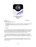
Approved for public release; distribution is unlimited.
Borehole X-Ray Fluorescence Spectrometer (XRFS):
User's Manual, Software Description,
and Performance Report
built by APL-UW under a NASA contract from the Langley Research Center
W.C. Kelliher1, I.A. Carlberg1, W.T. Elam2, and E. Willard-Schmoe2
1NASA Langley Research Center, Hampton, VA
2Applied Physics Laboratory, University of Washington, Seattle
Technical Report
CAUTION CAUTION CAUTION
APL-UW TR 0703
December 2007
This device produces
X-rays when energized.
CAUTION CAUTION CAUTION
Applied Physics Laboratory University of Washington
1013 NE 40th Street
Seattle, Washington 98105-6698
Contract NNL05AA49C
_______________________UNIVERSITY OF WASHINGTON • APPLIED PHYSICS LABORATORY_________________
Acknowledgments
This project was funded by NASA Headquarters as part of the Mars Technology
Program, Subsurface Access Task, administered by the Jet Propulsion Laboratory. We
are indebted to the program managers, Suparna Mukherjee and Chester Chu, for their
guidance. The XRF spectrometer design and construction were performed by the Ocean
Engineering Department of the Applied Physics Laboratory: Russ Light, Vern Miller,
Pete Sabin, Fran Olson, Tim Wen, and Dan Stearns. The performance reported here is
due to their efforts. The University of Washington effort was funded under NASA
contract NNL05AA49C.
i
TR 0703
_______________________UNIVERSITY OF WASHINGTON • APPLIED PHYSICS LABORATORY_________________
TR 0703
ii
_______________________UNIVERSITY OF WASHINGTON • APPLIED PHYSICS LABORATORY_________________
Contents
User’s Manual ...............................................................................................................1
Overview.....................................................................................................................1
Borehole XRFS Software Installation ........................................................................12
Instrument Design .....................................................................................................15
Typical Operation......................................................................................................19
Determining the Minimum Detection Limit (MDL) ...................................................40
Hardware Description.................................................................................................23
XRF Interface Unit....................................................................................................23
XRF Control Unit......................................................................................................26
Software Description ...................................................................................................29
X-ray Tube Control (XTC) ........................................................................................29
Detector Data Acquisition (DET) ..............................................................................31
Save and Load Parameters (PAR)..............................................................................33
Save and Load Spectrum (SSF) .................................................................................34
Spectrum Processing (SP)..........................................................................................36
Spectrum Display (SD)..............................................................................................36
Instrument Performance Report ................................................................................38
Materials and Methods ..............................................................................................39
Test Plan Summary....................................................................................................41
Results.......................................................................................................................42
Conclusions...............................................................................................................52
Appendices...................................................................................................................53
iii
TR 0703
_______________________UNIVERSITY OF WASHINGTON • APPLIED PHYSICS LABORATORY_________________
TR 0703
iv
_______________________UNIVERSITY OF WASHINGTON • APPLIED PHYSICS LABORATORY_________________
User’s Manual
Overview
The X-ray fluorescence spectrometer (XRFS) is designed to be deployed down a predrilled hole for exploration and elemental analysis of subsurface planetary regolith
(Figure 2 and Figure 10). The spectrometer excites atoms in the regolith and causes them
to emit their characteristic X-rays. These characteristic X-rays produce peaks in the Xray spectrum. By measuring the energy of the X-rays, elements are identified. By
measuring the intensity of the peaks, the amount of each element can be determined. A
software package operates the spectrometer, acquires the data, and analyzes the spectrum
to provide elements and their weight fractions. It also provides a user interface to control
the measurements and display the results.
Figure 1. X-ray fluorescence spectrometer Head Unit designed to be deployed down a pre-drilled
hole to analyze subsurface elements.
The spectrometer consists of two main subsystems packaged in three physical units. The
main subsystems are the X-ray source and the energy-dispersive X-ray detector. The
source provides the X-rays to excite the specimen of regolith being investigated. The
energy-dispersive X-ray detector detects the emitted X-rays, determines their energy (the
energy-dispersive function), and counts the X-rays at each energy. Together these two
subsystems measure the X-ray spectrum of the specimen.
1
TR 0703
_______________________UNIVERSITY OF WASHINGTON • APPLIED PHYSICS LABORATORY_________________
Quick Start Guide
Figure 2. (from left to right) Borehole XRFS Head Unit, X-ray warning light, umbilical cable, X-ray
Interface and Control units, and laptop computer.
Setup
To set up the instrument:
1. Remove the units from the case. The instrument consists of the XRF Interface
Unit, the XRF Control Unit, and the XRF Head Unit (Figure 2). A laptop
computer is used to control the instrument. There are three cables connecting the
Interface and Control units, and the Head Unit has an umbilical cable (15 ft.
long) permanently attached to connect it to the Control Unit. An X-ray warning
light is also supplied. The instrument must be used in a radiation safety enclosure
TR 0703
2
_______________________UNIVERSITY OF WASHINGTON • APPLIED PHYSICS LABORATORY_________________
or other personnel safety arrangement. An interlock cable connects to the safety
interlock switch on the radiation safety enclosure to prevent accidental exposure.
2. Connect the cables as shown in Figure 3. All cables must be connected before
turning on the main power.
3. Connect USB cable to the laptop computer and turn on the instrument with the
key switch. The laptop should beep when it recognizes the connection to the
instrument.
4. Wait one to two minutes for the detector to cool down. The instrument is now
ready to collect a spectrum.
3
TR 0703
_______________________UNIVERSITY OF WASHINGTON • APPLIED PHYSICS LABORATORY_________________
Figure 3. Connection diagrams for Interface, Control, and Head units of the XRF spectrometer.
TR 0703
4
_______________________UNIVERSITY OF WASHINGTON • APPLIED PHYSICS LABORATORY_________________
Spectrum collection
1. Place the sample to be analyzed before the probe window.
2. Close the radiation safety enclosure and be sure the interlock switch is closed.
3. Start the program “BoreholeXRF”; the main screen appears (Figure 4).
4. Turn on the high voltage to 35 kV, and the emission current to 2 µA.
5. Set the preset time to the desired interval.
6. Click “Start”.
7. The actual kV and µA values should be near the setting values (they may take one
or two minutes to reach these values because of the slow ramp).
8. “Acquiring” will appear in red on the screen (Figure 5).
9. A spectrum will begin to appear in the plot box in the lower left corner of the
interface (Figure 5).
10. To calibrate, click “Calibrate” and enter points in the form “channel number,
energy in keV” in the window that opens (Figure 6). Then click “Compute,” then
“Calibrate,” then “Close.” You may calibrate before, during, or after spectrum
collection.
11. To save the spectrum, click “Save.”
12. To determine which elements are present in the sample, click the “Analyze”
button. After several seconds, the plot box will show the background and
spectrum fits and the elemental analysis will appear in the spectrum analysis box
(Figure 7).
Software operation
Configuration settings:
•
“load params panel” (Figure 8): Opening this window allows the user to change
instrument control parameters (such as the ramp interval) and acquisition
conditions (such as the atmosphere type).
5
TR 0703
_______________________UNIVERSITY OF WASHINGTON • APPLIED PHYSICS LABORATORY_________________
•
“load DP4 config panel” (Figure 9): Opening this panel allows the setting for the
DP4 digital pulse processor to be changed. Refer to the AmpTek manual
(Appendix A) on the DP4 for more information about these parameters.
•
“on” and “off” under “X-ray control”: These buttons turn the X-rays on and off.
•
“setkV”: This button allows the user to set the high voltage for the X-ray tube.
•
“set µA”: This button allows the user to set the emission current.
•
“change preset time”: Use this button to enter the desired interval of data
collection in seconds, then click “OK.” This command automatically clears the
spectrum that is currently plotted (so save it first!). When the user clicks “Start”
after entering this preset time, the program will collect a spectrum and stop
automatically after the allotted time has elapsed. Note that this refers to
accumulation time, not live time.
“Input Spectrum” functions:
•
“Start”: Click this button to begin taking a spectrum.
•
“Stop”: Click this button to stop spectrum collection before the preset time has
elapsed.
•
“Clear”: This button clears the spectrum currently plotted.
•
“Calibrate”: The user may calibrate the energy of the spectrum any time before,
during, or after collection. It is also possible to load and calibrate a previously
saved spectrum. Click “Calibrate” to open the calibration window, enter the
desired channel-energy pairs (in keV) in the form “channel, energy,” click
“Compute,” “Calibrate,” and “Close.” It is also possible to type a desired energyper-channel value and energy start value manually and then click “Calibrate,”
without pressing “Compute.” The user may clear a previous calibration and
return to the original channel values by pressing “Remove calibration.”
TR 0703
6
_______________________UNIVERSITY OF WASHINGTON • APPLIED PHYSICS LABORATORY_________________
•
“Load”: This button allows the user to bring up a previously saved spectrum. It is
possible to enter a new spectrum label and operator, zoom in/out, calibrate,
analyze and re-save any previously saved spectrum.
Plot controls: (Note: none of these buttons affect data collection.)
•
“Restore”: Restores the spectrum plot to its original scale and causes it to begin
automatically adjusting the Y-scale to keep the entire spectrum in view.
•
“ cursor”: Moves the cursor one channel to the left.
•
“cursor ”: Moves the cursor one channel to the right.
•
“X zoom in”: Adjusts the X-scale so that it displays a smaller range of X values,
centered around the cursor.
•
“X zoom out”: Adjusts the X-scale so that it displays a larger range of X values,
centered around the cursor.
•
“X shift left”: Moves the view to the left approximately half of the plot range, so
that the user is looking at slightly lower energies.
•
“X shift right”: Moves the view to the right approximately half of the plot range,
so that the user is looking at slightly higher energies.
•
“Y zoom in”: Adjusts the Y-scale so that it displays a smaller range of Y values.
•
“Y zoom out”: Adjusts the Y-scale so that it displays a larger range of Y values.
“Analyze”: Click this button (after calibrating) to run an automated analysis of the
sample. It will return a list of elements present, their concentrations and
uncertainty.
“Save spectrum”: Allows the user to save the current spectrum and some configuration
information to a file on the computer. These files are accessible by the “load”
button in the Borehole XRF software, and can also be opened in a word
processing program or text editor.
7
TR 0703
_______________________UNIVERSITY OF WASHINGTON • APPLIED PHYSICS LABORATORY_________________
“Exit”: Exits the spectrum collection program. The program will not prompt the user to
save the current spectrum, so it is necessary to save (if desired) before exiting.
Figure 4. Main screen view upon starting the program “BoreholeXRF”
TR 0703
8
_______________________UNIVERSITY OF WASHINGTON • APPLIED PHYSICS LABORATORY_________________
Figure 5. View of laptop display during spectrum acquisition
Figure 6. View of calibration control window
9
TR 0703
_______________________UNIVERSITY OF WASHINGTON • APPLIED PHYSICS LABORATORY_________________
Figure 7. View of spectrum analysis display
TR 0703
10
_______________________UNIVERSITY OF WASHINGTON • APPLIED PHYSICS LABORATORY_________________
Figure 8. View of configuration setting “load parameters panel”
Figure 9. View of configuration setting “load DP4 configuration panel”
11
TR 0703
_______________________UNIVERSITY OF WASHINGTON • APPLIED PHYSICS LABORATORY_________________
Borehole XRFS Software Installation
Before connecting hardware, copy all files from CD-R folder titled “BoreholeXRF As
Shipped Bin Sept 27.2007.”
Place files in C:\Program Files\BoreholeXRF
(Note: the files MUST be in exactly this location to operate correctly.)
Necessary software files from the folder “BoreholeXRF As Shipped Bin Sept 27.2007”:
•
xrayxsct.dat
•
XRFanalysis.dll
•
APL_UW_XraySettings.xcg
•
asycfilt.dll
•
BoreholeXRF.exe
•
cbw32.dll
•
COMCAT.DLL
•
COMCT232.OCX
•
Comdlg32.ocx
•
dp4.cfg
•
MSCOMM32.OCX
•
msvbvm60.dll
•
oleaut32.dll
•
olepro32.dll
•
usbdrvd.dll
Install the driver for the Measurement Computing DAQ module.
•
Load the Measurement Computing “MCC DAQ Software” CD
•
Install InstaCal for Windows, TracerDAQ, and Hadware manuals
•
Install Shield Wizard for InstaCal – click “Next”
•
Destination Folder – click “Next”
TR 0703
12
_______________________UNIVERSITY OF WASHINGTON • APPLIED PHYSICS LABORATORY_________________
•
Ready to Install – click “Install”
•
Completed – click “Finish”
•
Install Shield Wizard for TracerDAQ – click “Next”
•
Destination Folder – click “Next”
•
Ready to Install – click “Install”
•
Completed – click “Finish”
•
User's Guides Setup – select “USB,” then click “Install”
(Driver is installed. This takes a few seconds.)
•
MCC DAQ message box – “You must restart your system...” – click “Yes”
After system has restarted, connect Borehole XRF hardware to USB port and turn power
on. “Found New Hardware Wizard” should appear.
“Can Windows connect to Windows Update...” – choose “No, not at this time.” – click
“Next”
Install software for DP4 Digital Pulse Processor (see also page 19 of Appendix A)
•
Select “Install from a list or specific location” – click “Next”
•
Select “Don't search, I will choose the driver to install” – click “Next”
•
Hardware type – Select “Human Interface Devices” – click “Next”
•
“Select the device driver...” – Click “Have disk...”
•
Insert the AmpTek CD into the CD drive
•
Click “Browse...”
•
“Install From Disk” file dialog appears
•
Navigate in the file dialog to:
My Computer\AMPTEK\USB_Driver\Win2k_XP\apausb2k.ini
•
Click “Open”
•
Back at the “Install From Disk” dialog – click “OK”
•
Back to “Select the device driver...” dialog – click “Next”
(Driver is installed. This takes a few seconds.)
13
TR 0703
_______________________UNIVERSITY OF WASHINGTON • APPLIED PHYSICS LABORATORY_________________
•
Completing installation – click “Finish”
Run the InstaCal program
•
From the menu bar, select: Start -> Programs -> Measurement Computing ->
Instacal
•
“Plug and Play Board Detection, USB-1408FS (Serial# 150)” should be selected
•
Click “OK”
•
Under the Install menu item, choose “Configure...”
•
Change No. of Channels from “4 Differential” to “8 Single Ended”
•
Click “OK”
•
Under the File menu item, choose “Exit”
Run the Borehole XRF program by double-clicking on the file “Borehole XRF.exe”
At this point the software main screen should appear; it will obtain a spectrum and bring
up all dialogs.
You may want to put a shortcut to the “Borehole XRF.exe” file on the desktop or some
other convenient location.
TR 0703
14
_______________________UNIVERSITY OF WASHINGTON • APPLIED PHYSICS LABORATORY_________________
Instrument Design
The instrument is designed to be deployed down a pre-drilled borehole and has a
maximum diameter of 27.1 mm to be compatible with existing drills (Figure 1 and Figure
10). The XRFS sensor assembly consists of an XRFS enclosed head assembly that is
deployed down the borehole and an electronics control assembly consisting of a power
supply and control electronics for the XRFS instrument. PC-based software provides the
control, data readout, and quantitative calculations needed for interpretation of the XRFS
spectra.
The excitation source is a silver anode X-ray tube (Comet NA, Stamford, CT) [see
Appendix B]. The energy dispersive X-ray detector is a 7-mm2 Si–PIN diode (Amptek,
Inc., Bedford, MA) [see Appendix C]. This detector was chosen mainly because of the
availability of a preamplifier compatible with the size restrictions. It has a good peak to
background ratio and a 12-micron thick beryllium window for light element sensitivity. A
digital pulse processor from the detector manufacturer (Amptek, Inc., Bedford, MA)
converts the detector output to an energy spectrum [see Appendix C]. The energy
calibration is linear and determined from the location of the iron characteristic emission
and silver elastic scatter peaks. Because the borehole diameter cannot be controlled with
precision, the collimation and beam definition geometry are optimized to allow for
varying distance to the measurement volume at the borehole wall. The excitation beam is
larger than the area viewed by the detector, making the signal less sensitive to the wall
distance.
The performance requirement is to detect the elements magnesium through zirconium
(atomic numbers 12 through 40 in the periodic table) and the elements cadmium through
15
TR 0703
_______________________UNIVERSITY OF WASHINGTON • APPLIED PHYSICS LABORATORY_________________
lead (atomic numbers 48 through 82 in the periodic table).
Figure 10. Engineering drawing of the final design of the downhole assembly. The enlarged area
shows the X-ray tube and the detector.
Major hardware subsystems
The X-ray source is a miniature but otherwise conventional X-ray tube. It generates Xrays by bombarding a metal anode with high-energy electrons. The electrons are
TR 0703
16
_______________________UNIVERSITY OF WASHINGTON • APPLIED PHYSICS LABORATORY_________________
produced in a hot filament and accelerated to high energy by a high voltage. The
filament heater power controls the beam, or emission, current. The X-ray output is
proportional to this current. The electron beam energy is controlled by the high voltage
applied to the X-ray tube. This voltage determines the X-ray spectrum emitted by the
tube and is one of the main parameters used to control the spectrometer. The X-ray tube
has a very high vacuum inside and the X-rays exit via a thin window. Other parameters
that influence the X-ray spectrum of the tube are the angles that the electron beam makes
with the anode and the exit window, the material and thickness of the exit window, and,
of course, the anode material.
The X-ray detector is based on a silicon diode that is reverse biased to provide a thick
region of high-resistivity silicon with an electric field across it. The X-rays are absorbed
in this region and produce electron–hole pairs in the silicon. The high electric field
separates the electron–hole pairs and produces a pulse of charge at the electrodes of the
diode. This pulse is amplified and its amplitude measured. Its amplitude is proportional
to the energy of the absorbed X-ray. A digital pulse processor separates this pulse from
the noise, determines its amplitude, digitizes the amplitude, and counts the pulses with
matching amplitudes to collect a spectrum.
The silicon diode is taken to about –60ºC by Peletier cooling to reduce the noise and
allow better resolution of the pulse amplitude. The energy resolution in the spectrum is
limited by the electronic noise in the diode and is typically about 150 electron volts. The
digital pulse processor is optimized for detecting and discriminating X-ray pulses from
this diode from the background noise. The count rate (the maximum rate that X-rays can
strike the detector) is limited to about 10,000 per second by the speed of the pulse
processing. The count rate is determined by the material being measured and the strength
of the X-ray source. The rate is typically adjusted by controlling the beam current in the
X-ray tube, as described above.
17
TR 0703
_______________________UNIVERSITY OF WASHINGTON • APPLIED PHYSICS LABORATORY_________________
Hardware physical units
The subsystems are packaged into three units: the XRF Head that goes down the
borehole and makes contact with the material being measured, the XRF Control Unit,
and the XRF Interface Unit.
The X-ray Head contains the X-ray tube and the silicon diode X-ray detector. It also has
a filament isolation transformer for the X-ray tube to isolate the filament heating power
from the high voltage. It contains a preamplifier for the detector to amplify the pulses
before they travel over the connecting cable. The X-ray Head is as small as possible to
go down the smallest pre-drilled hole and measure the composition of the regolith at
various depths. The 15-ft. umbilical cable is permanently attached to the Head Unit; it
connects the Head and Control units.
The XRF Control Unit contains all of the essential electronics to operate the X-ray tube
and detector. It constitutes the electronics that would be required for a future spacecraft
instrument. For the X-ray tube, there is the high voltage power supply (HVPS), the
filament driver and regulator, isolation amplifiers to provide monitor signals for the
voltage and current, and an over-current protection circuit. For the detector, the unit
contains a power supply board and the digital pulse processor board.
The XRF Interface Unit contains the hardware necessary to adjust and monitor the Xray tube voltage and current from the host computer, several interlock sensors for
personnel safety, and the low voltage power supplies for the electronics. This unit
contains all of the support equipment that is necessary to operate the spectrometer on the
ground. There are several cables connecting the XRF Interface and XRF Control units.
The XRF Interface Unit also connects to the host computer via USB, to the personnel
safety outerlocks, and to the main power line.
TR 0703
18
_______________________UNIVERSITY OF WASHINGTON • APPLIED PHYSICS LABORATORY_________________
The software described here interacts mainly with the data acquisition board used to
control the X-ray tube high voltage supply and with the digital pulse processor board for
the detector. These functions are described more fully beginning on page 26.
Typical Operation
A typical X-ray spectrum of terrestrial soil is shown in Figure 11. There are three
significant features. First are the large peaks in the spectrum between 3 and about 15
keV. These peaks are from the elements in the sample and are the main features of
interest. Second are the peaks between 15 and 20 keV. These are the characteristic peaks
from the X-ray tube anode material (silver in this case) that have been scattered toward
the detector by the sample. They can provide additional information but are not as
straightforward to interpret. The third feature is the background under the peaks. The
background is small in an XRF spectrum from a good spectrometer, allowing detection of
even very small peaks from elements at very low concentrations (the minimum detection
limit). However, it must be modeled and removed by the analysis algorithms to provide
accurate measurements of the peak intensities.
19
TR 0703
_______________________UNIVERSITY OF WASHINGTON • APPLIED PHYSICS LABORATORY_________________
Figure 11. Fluorescence spectrum taken with the borehole XRFS. The soil sample was JSC1A
Lunar Simulant.
Typical operation of the spectrometer by a user involves these steps. When power is
turned on, the X-ray source is off (not producing X-rays) and the detector starts to cool
down. The user places a specimen in front of the measurement window on the side of the
XRF head (or places the head in a borehole).
The user then closes a radiation safety enclosure. When the safety enclosure is closed, a
safety interlock switch closes, allowing the X-rays to be turned on. The voltage and
current for the X-ray tube are set at this time, or previous settings are read in and used.
The user chooses a data acquisition time, clears the spectrum in the digital pulse
processor (DPP), and starts data acquisition. The spectrum is displayed as it is collected
and the user will typically check the total count rate and make sure the spectrum looks
correct (perhaps examining some regions more closely using zoom and pan). The user
may be looking for particular elements, and will thus focus on the chosen elements. The
TR 0703
20
_______________________UNIVERSITY OF WASHINGTON • APPLIED PHYSICS LABORATORY_________________
user will then stop the data acquisition, change any data acquisition parameters to
optimize the spectrum, clear the spectrum, and collect the desired data.
The data are displayed as a function of the X-ray energy. To do this, the detector pulse
height must be calibrated to match the X-ray energies. This is typically done using X-ray
peaks from known elements. The calibration must be checked (typically daily) and may
need to be repeated at irregular intervals.
Once data are collected, they can be stored in a file and/or analyzed further. Further
analysis consists of modeling the background, finding any peaks in the spectrum and
associating them with the corresponding elements, determining the net intensity of the
peaks, and converting this net intensity into weight fractions of the elements. The
background and a reconstruction of the spectrum using the extracted net intensities are
displayed. This allows the user to quickly and visually evaluate the analysis of the
spectrum. The element list and weight fraction of each element, together with estimated
uncertainties, are also displayed.
The conversion from peak intensity to weight fraction is accomplished using a physical
model of the interaction of X-rays with the material being analyzed. This model requires
a complete description of the instrument to give accurate results. This description is
more information than is typically changed by the user, such as fixed angles and
distances within the components. It is also more information than the software needs to
control the instrument. This information is read in from a parameter file and is usually
not changed. It can be initially entered and changed via second-level dialogs that are
invisible unless needed.
The user can also enter information about the material being analyzed and can change the
instrument description information to be stored with the spectrum if desired. The data
21
TR 0703
_______________________UNIVERSITY OF WASHINGTON • APPLIED PHYSICS LABORATORY_________________
acquisition parameters, such at X-ray tube voltage and current, are automatically stored
with the spectrum.
The spectrum is stored in a file along with the information about the parameters under
which it was acquired and enough of a description of the instrument to allow later
analysis if necessary. The file format used is the standard format for energy-dispersive
spectra adopted by the Microscopy Society of America and the European Microscopy
Society.1 Additional keywords were added to provide a complete description of the
measurement conditions including instrument configuration (see Table 1).
1
European Microscopy Society standard format, Version 1.0, see files emmff.doc and emmff.src,
at http://www.amc.anl.gov/ANLSoftwareLibrary/02-MMSLib/XEDS/EMMFF/
There is a proposed format based on XML that is not yet standard. See file
EMSA_MAS_V2_XML_MM8_2002.pdf
TR 0703
22
_______________________UNIVERSITY OF WASHINGTON • APPLIED PHYSICS LABORATORY_________________
Hardware Description
XRF Interface Unit
Low voltage power supplies (COTS)
+/– 15 VDC for op-amps
+15 VDC, 1.5 amp for HV module
+5 VDC for interlocks and detector
Detector requires 0.5-A steady-state with 1-A startup surge lasting 30–60 sec.
DAQ and control board (COTS)
OnTrak ADR2000A
USB to serial adaptor (COTS)
Targus PA088
USB hub (COTS)
D-Link, Model DUB-H4, high-speed USB 2.0 4-port hub
Safety interlocks and control (APL-UW)
X-ray on/off
Purpose. Turns the X-ray tube on and off, including ramping filament up and
down and safety disabling the high voltage module.
Background. This signal controls the main functions of the X-ray tube power
supply system. It is disabled whenever one of the safety signals (see below) is
absent. It will shut down and latch in the “off” condition whenever one of the
safety signals disappears.
Operation. Logic circuit responds to a binary signal from the DAQ, tests all of
the safety condition signals, and provides signals for HV disable, filament voltage
ramp control, and status to the DAQ board.
23
TR 0703
_______________________UNIVERSITY OF WASHINGTON • APPLIED PHYSICS LABORATORY_________________
Warning light and fail-safe
Purpose. Controls the warning light (115 V AC external lamp), turning it on and
off with the X-rays. Provides a safety signal that indicates when the lamp is
working.
Background. One of the federal safety requirements for X-ray systems is a
warning light that turns on whenever the X-ray producing system is energized
(defined as high voltage on). The light must be fail-safe in that the X-rays will
not come on if the light bulb is burned out.
Operation. Solid-state relay to turn the power to the external socket on and off.
A current detector (full-wave bridge rectifier in parallel with Zener diodes driving
a 5-V DC relay) indicates that the external lamp is drawing current (i.e.,
connected and not burned out). The current detector does not provide a signal
unless the lamp is energized, a delay must be provided that allows the lamp to be
turned on, then X-rays must be turned off if the current detector does not indicate
lamp operation. The delay is typically about 100 milliseconds.
Electrical interlock status
Purpose. An external signal provided by a user that indicates that all of the X-ray
shielding is in place.
Background. Another federal safety requirement is that the enclosure that
protects human operators from radiation exposure be interlocked to the high
voltage supply. This interlock must disable the high voltage if the shielding is
opened, to prevent accidental radiation exposure.
TR 0703
24
_______________________UNIVERSITY OF WASHINGTON • APPLIED PHYSICS LABORATORY_________________
Operation. An external signal. It disables the high voltage power supply and
prevent X-rays from being turned on (or shut them off if they are on). The signal
is typically an external switch closure. It also disables the X-rays in case of a
short to ground to prevent shorts from giving a false OK signal. A TTL or other
logic signal is OK if +5 V or similar is available on the external connector to
facilitate use with un-powered mechanical switches on a radiation enclosure.
Filament connector engaged
Purpose. To insure that the filament connector is inserted before the high voltage
or X-rays are turned on.
Background. The commercial, miniature high voltage connectors used have only
a contact for the negative high voltage, not for the positive return path (ground in
this case). The ground return path is via the filament connector. If the high
voltage is energized with the high voltage connector in place and the filament
connector dangling, then a shock hazard condition can be produced.
Operation: A simple logic circuit that passes through the external filament
connector via two extra pins.
Over-current signal
Purpose: See over-current cutoff under high voltage power supply board in the
XRF Control Unit above. This signal is passed through to the DAQ and should
remain after the X-rays are turned off until reset via the DAQ (usually by the Xrays off signal).
Background. This is just an interface to the over-current cutoff from the high
voltage power supply board.
25
TR 0703
_______________________UNIVERSITY OF WASHINGTON • APPLIED PHYSICS LABORATORY_________________
Operation. Logic circuit that is part of the X-ray on circuit.
Ground failure detect
Purpose. Insures that a safe return path for the high voltage exists and avoids
potential shock hazards.
Background. If high voltage is applied to the X-ray tube and a connection
between the X-ray tube anode and the return current path to the power supply
ground fails, then a potential shock hazard exists. This circuit tests the ground
return path by applying a voltage to the X-ray tube anode via a resistor, then
testing to be sure that voltage is shorted to ground.
Operation. Applies a voltage through a pair of resistors, to the X-ray tube anode
over the umbilical cable. One resistor is in the power supply and one is in the
XRF Head Unit near the X-ray tube anode. This will produce a known voltage if
the X-ray tube is properly grounded. If the umbilical cable lead is shorted, then
the voltage will be zero. Provides a signal if the correct voltage is present, and
disable the X-rays if not.
XRF Control Unit
High voltage power supply board
HV module (COTS)
Filament driver and regulator (APL-UW)
Purpose. Provides AC drive voltage for filament isolation transformer to heat
filament. Regulates filament voltage to achieve emission current set point.
TR 0703
26
_______________________UNIVERSITY OF WASHINGTON • APPLIED PHYSICS LABORATORY_________________
Background. The electron beam in an X-ray tube is generated from a hot
filament at high negative voltage. The electrons emitted from the hot filament are
accelerated by the high voltage and strike a metal anode at ground potential. The
metal anode emits X-rays. The filament is heated by a current passing through
the filament wire. Since the filament is at high negative potential, the heater
current must be isolated by a filament transformer operating at 6 kHz. The
electron beam current is regulated by the temperature of the filament, which is
controlled by the filament heater current.
Operation. 6-kHz AC is generated by an oscillator, whose output voltage is
controlled by a feedback loop. The output goes to a power audio amplifier chip to
produce enough power and voltage to drive the filament transformer (which is
located in the XRF Head). The feedback loop compares the current signal from
the HV module to a set point and adjusts the filament heater voltage. The
feedback has upper and lower limits (via a Zener diode), integration of the error
signal (via a capacitor), and some linear gain for stability (via a resistor), all in the
feedback leg of an op-amp. This regulator reverts to the “filament off” condition
on power-up and wherever X-rays are turned off.
Isolation and amplification of HV monitor signal (APL-UW)
Purpose. To condition the signals from the HV module to achieve convenient
gain and to protect the remainder of the circuits from spikes due to high voltage
arcs.
Operation. Op-amps with diode and capacitor spike suppression at their inputs.
27
TR 0703
_______________________UNIVERSITY OF WASHINGTON • APPLIED PHYSICS LABORATORY_________________
Over-current cutoff (APL-UW)
Purpose. To protect all of the hardware from a long-term overload condition.
Background. X-ray tubes sometimes develop arcs or plasma discharges. If they
are brief, they usually clear themselves and are not a problem. But if they last for
several seconds, they can overheat themselves or other components. This
protection circuit serves as a backup to the software over-current protection. The
HV module is also current-limited, but that only protects the module, not the Xray tube.
Operation. Compares the emission current signal from the HV module to an onboard set point. If the emission current exceeds the set point for more than 5 sec,
turn off the X-rays.
Detector power board (COTS)
AmpTek PC4-3
Detector pulse processor board (COTS)
AmpTek DP4. The detector system is completely isolated as well as electrically
and magnetically shielded from the X-ray tube power supply, with one common
ground point at the +5 volt power supply. The signals from the X-ray detector at
the preamp output are pulses of about 10 microseconds duration and about 1 mV
amplitude. Their amplitude must be measured to within a few percent to obtain a
useable X-ray spectrum. Electronic noise is the major limitation and is
minimized. Magnetic shielding is accomplished with co-netic foil.
TR 0703
28
_______________________UNIVERSITY OF WASHINGTON • APPLIED PHYSICS LABORATORY_________________
Software Description
X-ray Tube Control (XTC)
Description
This module has two main purposes: to display and allow the user to change the
parameters related to the X-ray tube, and to control the high-voltage power supply
(HVPS) for the X-ray tube. The controls for this module are located on the main screen
in the upper right corner of the interface (Figure 4).
The main parameters for the X-ray tube are the high voltage (kV) and the beam emission
current (µA). Typical values are 35 kV and 2 µA. The user must also input a complete
description of the X-ray tube for proper operation of the quantitative analysis software.
These parameters are in a separate dialog that appears on request but is usually invisible
(Figure 8).
The HVPS has a series of safety interlocks to prevent accidental exposure of personnel to
high electrical voltages and X-ray radiation. The status of these interlocks is clearly
visible to the user and turn red if any fail (Figure 12).
Control of the HVPS requires turning the X-ray on and off under user control, and
responding to any changes in the interlock status by turning off the X-rays. The X-ray
tube voltage and current settings are converted from the display units (kV and µA) to the
DAC integer values and sent to the DAC using its commands. The actual values are read
from the DAC and converted to the display units. When the X-rays are turned on, the Xray tube must be ramped up to the operating conditions gradually (see ramp-up under
functions).
29
TR 0703
_______________________UNIVERSITY OF WASHINGTON • APPLIED PHYSICS LABORATORY_________________
Figure 12. Borehole XRF interface indicating interlock failure
Functions
Set and display X-ray tube voltage (kV)
Set and display X-ray tube emission current (µA)
Check limits for X-ray tube parameters
Check and display status of safety interlocks
•
X-ray on/off
•
Warning light and fail-safe
•
Electrical interlock
•
Filament connector engaged
•
Over-current signal
•
Ground failure detect
Turn X-rays on and off
TR 0703
30
_______________________UNIVERSITY OF WASHINGTON • APPLIED PHYSICS LABORATORY_________________
Ramp-up X-ray tube gradually to full operation
•
Bring up kV to no more than 10 kV
•
Bring up emission current to no more than 5 µA
•
Raise kV and µA gradually together to specified values
Communicate with HVPS
•
USB port or other communication parameters
•
Commands to ADC and DAC
•
ADC and DAC conversion constants
Set and display X-ray tube and instrument description
•
X-ray tube type (side or end window)
•
Anode material
•
Be window thickness
•
Electron incident angle
•
Takeoff angle
•
Aperture size and distance
•
Filter material and thickness (if any)
•
Path length from X-ray tube to specimen
•
Angle that X-rays from tube strike specimen (incidence angle)
Detector Data Acquisition (DET)
Description
The X-ray detector acquires the spectrum; its associated electronics are commercial offthe-shelf. The manufacturer (Amptek, Inc., Bedford, MA) also supplies a library of
communications and control routines that operate over a USB interface. The main
function of the DET module is to drive these functions to acquire the spectrum (once the
X-ray tube is operating and the user requests data be collected). As with the X-ray tube,
31
TR 0703
_______________________UNIVERSITY OF WASHINGTON • APPLIED PHYSICS LABORATORY_________________
there are several data acquisition parameters that the user can change. Some of these
appear on the main screen and some in a separate dialog (Figure 9).
The signal from the X-ray detector is analyzed by a digital pulse processor (DPP) that is
specialized for energy-dispersive X-ray detector pulses. Many of the parameters for this
DPP are software changeable but require specialized commands and some tuning
procedures. The parameters are loaded at startup from a database.
One of the auxiliary functions of the detector data acquisition module is to check, set, and
maintain the detector energy calibration (Figure 6). This calibration relates the channels
in the spectrum (which are proportional to the pulse amplitude from the detector) to Xray energy. The calibration is determined using the peaks of known elements, either in
the spectrum from the material of interest if they are known or from a calibration sample.
The energy calibration procedure consists of finding the location of the peaks, identifying
the element associated with the peak, and including the peak positions and element
energies in a calibration function. The function used is linear. The energy calibration
will usually not change much day-to-day, so a stored calibration can be used. Any
changes in the DPP tuning will change the calibration, so the DPP setup and calibration
will force a re-calibration if any DPP parameters are changed.
Functions
Communicate with detector digital signal processor (COTS code)
Set and display data acquisition parameters
TR 0703
•
Live time (seconds, calculated in DPP)
•
Real time (seconds)
•
Count rate (counts per second, display only)
•
Dead time (%, display only)
•
Total counts (display only)
32
_______________________UNIVERSITY OF WASHINGTON • APPLIED PHYSICS LABORATORY_________________
•
Chamber atmosphere (Earth ambient, Mars ambient, pure helium,
vacuum)
Energy calibration (eV per spectrum channel)
•
Set and display calibration constants
•
Calculate energy vs. channel (linear or quadratic function)
Set and display detector parameters
•
Aperture size and distance
•
Path length from specimen to detector
•
Energy resolution
•
Window material and thickness
•
Dead layer material and thickness
•
Active layer material and thickness
•
Angle that X-rays exit specimen toward detector (emergence angle)
Set and display digital pulse processor parameters
•
(See manufacturer’s manual, Appendix A)
Control digital pulse processor setup
Save and Load Parameters (PAR)
Description
This module handles all the parameters from other modules. The functions in this module
are called at startup and shutdown, and by the other modules whenever any parameters
are changed.
The module saves the parameters to a file and reads them from a file. The name and
location of the parameter file are set and displayed by this module via a dialog (Figure 8).
No other parameters are modified or displayed by this module. The file format is
determined and controlled by this module.
33
TR 0703
_______________________UNIVERSITY OF WASHINGTON • APPLIED PHYSICS LABORATORY_________________
Functions
Set and display parameter file name
Save all parameters to file
Load all parameters from file
Save and Load Spectrum (SSF)
Description
The spectrum is stored in a file that contains the spectrum data (counts per channel), the
energy calibration that relates channels to X-ray energy, the parameters under which it
was acquired, and the description of the instrument. Older files can be read in by the
software and displayed and analyzed just as newly collected data are handled. All of the
information necessary to display the spectrum and to allow later re-analysis if desired is
stored in the spectrum file.
Functions
Set and display spectrum file name
Save data and all relevant parameters to file
Load data and all relevant parameters from file
File format
The file format is the standard format for energy-dispersive spectra adopted by the
Microscopy Society of America and the European Microscopy Society.2 Additional
2
European Microscopy Society standard format, Version 1.0, see files emmff.doc and emmff.src,
at http://www.amc.anl.gov/ANLSoftwareLibrary/02-MMSLib/XEDS/EMMFF/
There is a proposed format based on XML that is not yet standard. See file
EMSA_MAS_V2_XML_MM8_2002.pdf
TR 0703
34
_______________________UNIVERSITY OF WASHINGTON • APPLIED PHYSICS LABORATORY_________________
keywords (Table 1) were added to this format to allow inclusion of the instrument
parameters used to analyze the spectrum.
Table 1. Keywords for XRFS spectrum output and parameter files added to the standard format
for energy-dispersive spectra
Keyword
kVsetting
uAsetting
kVscaleIn
kVoffsetIn
uAscaleIn
uAoffsetIn
uAdividerR
kVscaleOut
kVoffsetOut
uAscaleOut
uAoffsetOut
RampInterval
kVdelta
uAdelta
kVstart
kVlimit
uAlimit
anode_z
kv
tube_inc_angle
tube_takeoff_angle
tube_be_window
filter_z
filter_thick
excit_angle
emerg_angle
solid_angle
path_type
inc_path_length
emerg_path_length
window_type
window_thick
minimum_energy
Description
X-ray tube kiloVolts Setting
X-ray tube microAmps Setting
kV Input Scale
kV Input Offset
uA Input Scale
uA Input Offset
uA Divider resistance (gigaOhm)
kV Output Scale
kV Output Offset
uA Output Scale
uA Output Offset
Ramp Interval (sec)
kV Ramp Delta
uA Ramp Delta
Minimum kV for Filament Start
kV Limit
uA Limit
X-ray tube anode atomic number
X-ray tube kiloVolts during acq.
X-ray tube electron incident angle
X-ray tube takeoff angle
X-ray tube Be window (mm)
Incident beam Filter atomic number
Incident beam Filter thickness (micron)
Incident beam Excitation angle (deg)
Fluorescence Emergence angle (deg)
Solid Angle (sterdian)
Atmosphere Path type
Incident path length (cm)
Emergence path length (cm)
Probe Window type
Probe Window thickness (micron)
Minimum analysis energy (eV)
35
Default value
20.00000000
5.00000000
-9.56999969
0.00000000
24.50000000
0.01000000
0.40500000
0.09380000
-0.14000000
0.04100000
0.10000000
1.00000000
1.00000000
5.00000000
10.00000000
40.00000000
25.00000000
47.00000000
20.21008301
90.00000000
51.11999893
0.50000000
1.00000000
0.00000000
38.86999893
74.12000275
0.00000850
2.00000000
0.94000000
1.97000003
2.00000000
0.00000000
1000.00000000
TR 0703
_______________________UNIVERSITY OF WASHINGTON • APPLIED PHYSICS LABORATORY_________________
Spectrum Processing (SP)
Description
This module calls another written in C++ to handle all of the computations. The
parameters needed by the physical model contained in the code are provided by the
spectrum processing module to the C++ module. The results of the spectrum analysis are
provided to the user in an on-screen list and to the spectrum display module. This
includes the calculated background and peak fits, the list of elements found in the
spectrum, and the weight fractions of each element with associated uncertainties (Figure
7). Net intensities of the associated peaks for each element are also displayed with the
intensity error from the Poisson statistics of the spectrum in the list on the lower right
corner of the interface.
The element identification and association of peaks with elements is fully automated but
is not entirely reliable. The quantitative results can be copied to the clipboard and made
available outside the program to prepare reports using the results of this instrument.
Functions
Background calculation and removal
Peak search
Element identification (associate peaks with elements)
Net peak intensity determination and calculated peak fits
Quantitative analysis (converting peak intensity to element weight percent)
Copy results to display
Spectrum Display (SD)
Functions
Plot spectrum vs. X-ray energy (Figure 5)
Overlay calculated background and peak fits
TR 0703
36
_______________________UNIVERSITY OF WASHINGTON • APPLIED PHYSICS LABORATORY_________________
Display markers at characteristic element emission line energies
Scale, zoom, and pan
37
TR 0703
_______________________UNIVERSITY OF WASHINGTON • APPLIED PHYSICS LABORATORY_________________
Instrument Performance Report
The purpose of this instrument is elemental analysis of regolith strata in a pre-drilled
borehole to investigate the subsurface of Mars and possibly other bodies within the solar
system. As such the primary performance criterion is the ability to quantify the elements
present in a particular stratum in an acceptable time and with sufficient accuracy to obtain
useful scientific information. For the purposes of this study, the detailed performance of
the sensor was evaluated by measurements on the actual prototype. The main
performance metric is the minimum detection limit (MDL). Improvements in the ability
to detect an element imply improvements in the ability to quantify the amount present.
Though there are some subtleties in this, the performance is dominated by the number of
X-rays present in the spectrum, which is dominated by the source strength given the
constraints on geometry and the available detectors for this instrument. The performance
was evaluated by measuring the detection limits of target elements in a light element
matrix.
The ability to accurately quantify a particular element is mainly limited by the precision
with which its X-ray emissions can be measured. This is determined by the statistical
variations in X-ray intensity due to the Poisson nature of their arrival times. In a given
time interval the number of X-rays that are detected has an intrinsic variance (the square
of the standard deviation) equal to the number of X-rays. This means that the relative
standard deviation is one over the square root of the number. For a given geometry and
sample composition, the number of X-rays detected from a particular element is
proportional to the source strength and the measurement time.
Detecting an element depends on both the number of X-rays collected from that element
and the background present even in the absence of that element. Because the background
is also subject to the same variations, the MDL is usually taken as three times the
TR 0703
38
_______________________UNIVERSITY OF WASHINGTON • APPLIED PHYSICS LABORATORY_________________
standard deviation of the background (converted to elemental concentration by an
appropriate calibration coefficient). This is equal to three times the square root of the
background counts in the spectrum. Both the desired signal and the background are
proportional to the source strength. The background arises from scatter of the continuum
from an X-ray tube and the detector peak-to-background ratio.
Materials and Methods
Standard Reference Materials
Standard Reference Materials (SRMs) numbered 2709, 2710, 2711, 97B and 2702 from
the National Institute of Standards and Technology were used for the characterization
tests. These SRMs are a set of selected soils with varying amounts of the basic soil
elements and extra elements in the form of contaminants. Concentrations ranged from
tens of percents for the basic soil components to below one part per million. This
provided a wide range to evaluate the instrument.
Samples were received from the National Institute of Standards and Technology as fine
powders. The samples were poured into specimen cups as received and presented to the
instrument without further preparation. Mars environmental conditions were simulated
on a laboratory bench-top using a glove bag. Eight millibar carbon dioxide partial pressure
was chosen as representative of the Mars atmosphere. A gas mix of three volume percent
carbon dioxide with helium making up the balance at Earth ambient pressure and gravity
provided the same carbon dioxide density typical of Mars atmosphere. All measurements
were made in this atmosphere.
39
TR 0703
_______________________UNIVERSITY OF WASHINGTON • APPLIED PHYSICS LABORATORY_________________
Determining the Minimum Detection Limit (MDL)
A spectrum is collected of a known sample containing the element for which the MDL is
desired. It is best to use a sample with a known element concentration less than 100
times the MDL. The largest peak from the element is found (usually K α or L α) and the
background is determined by a linear fit to the spectrum on either side of the peak. To
determine the total background counts the number of channels under the peak is
multiplied by the average counts in the channels on either side of the peak. The gross
peak counts are similarly determined by summing the counts in all channels under the
peak. The net counts from the element are the gross counts in the peak minus the total
background counts. Next the square root of the total background counts is multiplied by
three, then multiplied by the ratio of the known element concentration to the net counts
from the element. This yields the MDL in the same units as the known concentration.
Note that this procedure assumes a linear relationship between net counts and
concentration, which is a good assumption at low concentrations near the MDL. All
MDLs given in this instrument performance report were calculated using this procedure.
TR 0703
40
_______________________UNIVERSITY OF WASHINGTON • APPLIED PHYSICS LABORATORY_________________
Figure 13. Raw spectra of five SRMs acquired with the borehole XRFS.
Test Plan Summary
•
Determine the MDL for the elements Mg, Zr, Cd, and Pb
•
Measure power consumption during spectrum collection
•
Dry, water saturated, and frozen sample
•
Variation with distance to probe (in case borehole diameter is not constant)
•
Measurement stability vs. time
•
Calibration linearity
41
TR 0703
_______________________UNIVERSITY OF WASHINGTON • APPLIED PHYSICS LABORATORY_________________
Results
Figure 14 shows typical spectra from the borehole instrument. The specimen was a
terrestrial soil, SRM 2709, measured in the Mars simulated atmosphere. The silver target
X-ray tube was operated at 35 kV and 2 µA. No filters or other optics were used in the
incident beam. The detector has an internal collimator to restrict the beam to the center of
the diode. Data collection time was 1000 sec for the upper spectrum and 100 sec for the
lower spectrum. Note that the majority of the information is still available even with the
100-sec data collection time. This short data collection will greatly facilitate the
measurement of multiple strata in a borehole with vertical resolution of about 1 cm.
Figure 14. Spectra from borehole XRF spectrometer. Upper curve is 1000-sec data collection
time, and lower curve is 100 sec.
TR 0703
42
_______________________UNIVERSITY OF WASHINGTON • APPLIED PHYSICS LABORATORY_________________
As a comparison, the APXS (alpha proton X-ray spectrometer) spectra used on the
Pathfinder and MER rovers have little usable data above the iron peaks at 6.4 keV (Figure
15). The spectrum acquisition times for both APXS curves were many hours. The scale
is counts per second, so 1 corresponds to about 72,000 total counts.
3
Figure 15. Spectra from the APXS instrument. Reproduced with permission.
Detection limits for a number of elements in parts per million are presented in Table 2.
They are computed using the three sigma method and assuming a linear relationship
between net counts and the certified concentration. The background was linearly
interpolated from the counts on either side of the peak. Detection limits for each SRM
3
R. Reider, R. Gellert, J. Brückner, G. Klingelhölfer, G. Driebus, A. Yen, and S.W.
Squyres, J. Geophys. Res., 2003, 108, 8066–8078, DOI:10.1029/2003JE002150.
43
TR 0703
_______________________UNIVERSITY OF WASHINGTON • APPLIED PHYSICS LABORATORY_________________
are given, along with the average values. SRM 2710 has rather high concentrations of
many of the elements, so the linear concentration relationship may not hold. This causes
the detection limits to be larger in this material. They were included in the averages since
they have the effect of raising the detection limits, and including them avoids any bias
toward lower values.
None of the SRMs contained Mg at a level that gave an unambiguous peak. A compound
with magnesium as a major element was used to determine the magnesium detection limit.
Talc, or magnesium silicate hydroxide, is a readily available magnesium compound (as
baby powder, obtained from a local pharmacy) and was used for this purpose. Lowering
the X-ray tube voltage to 20 kV decreased the magnesium detection limit from about 3%
to the 1.4% value (Table 2). The ability to change the excitation conditions is another
strong argument for using an X-ray tube.
Measured power consumption is given in Table 3 for the system components and the
total. Ground support components including the safety interlocks and the USB computer
interface are not included, as these functions are either not necessary in a spacecraft or are
expected to be provided. The total power of 12 watts implies an energy requirement of
12 kJ per spectrum for a 1000-sec spectrum or 1200 J for a 100-sec spectrum. This is
comparable to the APXS energy per spectrum, with larger power consumption but
shorter collection times.
TR 0703
44
_______________________UNIVERSITY OF WASHINGTON • APPLIED PHYSICS LABORATORY_________________
Table 2. Minimum detection limits for several elements
Element
2702
2709
2710
2711
97B
Average
Mg
ND
ND
ND
ND
ND
1.4%
Ni
ND
8.9
2.0
ND
NP
5.5
Cu
8.2
4.2
16.2
8.9
NP
9.4
Zn
8.0
6.6
16.9
8.3
6.4
9.2
Pb
8.8
3.3
22.0
12.4
NP
11.6
NP
4.5
NP
4.1
4.8
4.5
Zr
ND = Not Detected
*
NP = None Present
Table 3. Power consumption during data collection
Function
Voltage
Current
Power
HV Power Supply
+14.84 V
0.426 A
6.31 W
X-ray tube control
+14.92 V
-14.92 V
+4.99V
0.150 A
0.149A
0.240A
4.46 W
Detector
Total
1.20 W
11.97 W
The effect on the measured spectrum from the presence of water is shown in Figure 16,
where spectra from dry, water saturated, and frozen specimens of SRM 2702 are
overlaid. There is almost no change in peak intensities, which is expected and indicates
that good quantitative information can be obtained regardless of water content. Also, the
presence of water will cause no significant degradation of detection limits. The region of
the spectrum that has peaks from coherent (Rayleigh) and incoherent (Compon) scatter
from the characteristic emission lines of the silver X-ray tube is shown in more detail in
Figure 17. Note that the scatter is much larger in the saturated and frozen specimens.
This increased scatter indicates presence of water and can be used to quantify the amount
of water present.
45
TR 0703
_______________________UNIVERSITY OF WASHINGTON • APPLIED PHYSICS LABORATORY_________________
Figure 16. Spectra of dry, water saturated, and frozen samples of SRM 2702. (Frozen spectrum
is 100 seconds to avoid thawing. It is multiplied by 10 for comparison.)
TR 0703
46
_______________________UNIVERSITY OF WASHINGTON • APPLIED PHYSICS LABORATORY_________________
Figure 17. Spectra of dry, water saturated, and frozen samples of SRM 2702. (Frozen spectrum
is 100 seconds to avoid thawing. It is multiplied by 10 for comparison.)
47
TR 0703
_______________________UNIVERSITY OF WASHINGTON • APPLIED PHYSICS LABORATORY_________________
Figure 18. Variation in fractional change of total spectrum counts and iron intensity with distance
to probe. Tests conducted with SRM 2711. Note different scales.
TR 0703
48
_______________________UNIVERSITY OF WASHINGTON • APPLIED PHYSICS LABORATORY_________________
The results of varying the distance from the probe to the sample are given in Figure 18.
The intensity in the iron peak and the total counts in the spectrum are plotted as a
function of separation between the probe body and the sample surface. The plot on the
left shows the behavior in the first few millimeters and the plot on the right shows all of
the data taken for this test. Note that both of these measurements are stable to within 2%
for as much as 2 mm of separation. In addition, the normalized iron intensity, which is
the ratio of the iron peak to the total counts, is plotted as the green line. This quantity is
stable out to almost 5 mm, indicating that accurate quantitation can be performed even at
this distance. This is important since the diameter of the borehole may not be constant
and thus the distance between the probe and the regolith being measured may vary.
Because of the design, these expected variations will not affect the results of they are less
than 2 mm and can be compensated for out to 5 mm. Beyond 10 mm the spectrum is no
longer a reliable measurement of the sample.
49
TR 0703
_______________________UNIVERSITY OF WASHINGTON • APPLIED PHYSICS LABORATORY_________________
Figure 19. Variation in total spectrum counts over one week. (Point on Day 2 is after instrument
was in continuous operation for 4 hr.)
Results of the measurement stability test are given in Figure 19. Stability is about 2%
except for the final point. It is now known why this point is an outlier. The two points
on day 1 were taken when the instrument was first powered on and after several hours of
operation.
The calibration linearity was checked by plotting the composition measured by the
instrument against the certified composition for all elements in all of the SRMs (below 10
weight percent) (Figure 20). Except for two outliers and several false positives (the
points above the line near zero composition), the calibration is very good. The analysis
algorithm used here is a “standardless” algorithm that relies entirely on the fundamental
TR 0703
50
_______________________UNIVERSITY OF WASHINGTON • APPLIED PHYSICS LABORATORY_________________
parameters method to obtain the weight percent from the intensities in the spectrum. No
standards were used in calculating these results. This is an advanced method that is not as
good as careful use of type-specific standards, but was incorporated into the probe
software because standards that are similar to the planetary regolith may not be available,
especially if the subsurface regolith composition is unknown. Further work on the
fundamental parameters analysis algorithm should improve the calibration performance.
For the best results, appropriate standards with certified compositions can be used with
an empirical correction algorithm.
Figure 20. Measured vs. given composition for a wide range of elements in all five standard
reference materials.
51
TR 0703
_______________________UNIVERSITY OF WASHINGTON • APPLIED PHYSICS LABORATORY_________________
Conclusions
A borehole X-ray fluorescence spectrometer (XRFS) has been successfully constructed
and tested. Miniaturization has been performed to a diameter of 27.1 mm and
components can be configured in a variety of XRFS instrument designs. Modifications
can be easily incorporated, such as an SDD detector, the use of a different target X-ray
tube, or use of radioactive sources for excitation. Performance is very good, with
detection limits of about 10 ppm for many elements and detection of light elements down
to magnesium at 1.4%. Power consumption is 12 watts during data collection and the
total energy per spectrum is comparable to previous planetary inorganic analysis
instruments. Adequate data can be collected in 100 sec, facilitating investigation of strata
with vertical resolution of about 1 cm in a reasonable time.
TR 0703
52
_______________________UNIVERSITY OF WASHINGTON • APPLIED PHYSICS LABORATORY_________________
Appendices
All appendices are available on the CD-R that accompanies this report.
Appendix A. Digital Pulse Processor: User’s Guide and Operating
Instructions
Appendix B. X-ray Tube Product Documentation
Appendix C. Detector specification sheet
Appendix D. Borehole XRFS wiring diagrams
Appendix E. Borehole XRFS safety interlock/control board schematic
Appendix F.
Borehole XRFS HVPS power and control board schematic
Appendix G. Borehole XRFS head unit and umbilical cable schematics
Appendix H. Borehole XRFS safety interlock/control board layout
Appendix I.
Borehole XRFS HVPS power and control board layout
Appendix J.
Bill of materials for safety interlock control
Appendix K. Bill of materials for HVPS power and control board
Appendix L.
Borehole XRFS detector interface board schematic
Appendix M. Borehole XRFS detector interface board layout
Appendix N. Borehole XRFS safety controller software program by Peter
Sabin
53
TR 0703
Form Approved
OPM No. 0704-0188
REPORT DOCUMENTATION PAGE
Public reporting burden for this collection of information is estimated to average 1 hour per response, including the time for reviewing instructions, searching existing data sources, gathering and maintaining
the data needed, and reviewing the collection of information. Send comments regarding this burden estimate or any other aspect of this collection of information, including suggestions for reducing this
burden, to Washington Headquarters Services, Directorate for Information Operations and Reports, 1215 Jefferson Davis Highway, Suite 1204, Arlington, VA 22202-4302, and to the Office of Information
and Regulatory Affairs, Office of Management and Budget, Washington, DC 20503.
1. AGENCY USE ONLY (Leave blank)
2. REPORT DATE
3. REPORT TYPE AND DATES COVERED
December 2007
Technical Report
5. FUNDING NUMBERS
4. TITLE AND SUBTITLE
Borehole X-Ray Fluorescence Spectrometer (XRFS): User's Manual,
Software Description, and Performance Report
NNL05AA49C
6. AUTHOR(S)
W.C. Kelliher, I.A. Carlberg, W.T. Elam, and E. Willard-Schmoe
8. PERFORMING ORGANIZATION
REPORT NUMBER
7. PERFORMING ORGANIZATION NAME(S) AND ADDRESS(ES)
Applied Physics Laboratory
University of Washington
1013 NE 40th Street
Seattle, WA 98105-6698
APL-UW TR 0703
9. SPONSORING / MONITORING AGENCY NAME(S) AND ADDRESS(ES)
10. SPONSORING / MONITORING
AGENCY REPORT NUMBER
Cedric Mitchener
Office of Procurement, Research & Projects Contracting Branch
Mail Stop 126
9B Langley Blvd.
Hampton, VA 23681-2199
11. SUPPLEMENTARY NOTES
12a. DISTRIBUTION / AVAILABILITY STATEMENT
12b. DISTRIBUTION CODE
Approved for public release; distribution is unlimited
13. ABSTRACT (Maximum 200 words)
The X-ray fluorescence spectrometer (XRFS) is designed to be deployed down a pre-drilled hole for exploration and elemental
analysis of subsurface planetary regolith. The spectrometer excites atoms in the regolith and causes them to emit their characteristic X-rays. These characteristic X-rays produce peaks in the X-ray spectrum. By measuring the energy of the X-rays,
elements are identified. By measuring the intensity of the peaks, the amount of each element can be determined. A software
package operates the spectrometer, acquires the data, and analyzes the spectrum to provide elements and their weight fractions.
It also provides a user interface to control the measurements and display the results.
The spectrometer consists of two main subsystems packaged in three physical units. The main subsystems are the X-ray source
and the energy-dispersive X-ray detector. The source provides the X-rays to excite the specimen of regolith being investigated.
The energy-dispersive X-ray detector detects the emitted X-rays, determines their energy (the energy-dispersive function), and
counts the X-rays at each energy. Together these two subsystems measure the X-ray spectrum of the specimen.
14. SUBJECT TERMS
Mars, spectrometry, regolith, X-ray fluorescence, XRF, elemental analysis, inorganic analysis,
borehole
17. SECURITY CLASSIFICATION
OF REPORT
Unclassified
NSN 7540-01-280-5500
18. SECURITY CLASSIFICATION
OF THIS PAGE
Unclassified
19. SECURITY CLASSIFICATION
OF ABSTRACT
Unclassified
15. NUMBER OF PAGES
57 + CD-R
16. PRICE CODE
20. LIMITATION OF ABSTRACT
SAR
Standard Form 298 (Rev. 2-89)
Prescribed by ANSI Std. 239-18
299-01