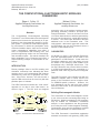
1
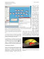
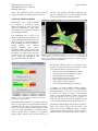
Applied Research Associates
4690 Millennium Drive, Suite 210
Belcamp, MD 21017
(410) 272-8862
THE COMPUTATIONAL ELECTROMAGNETIC MODELING
FRAMEWORK
Edgar L. Coffey, III
Applied Research Associates, Inc.
[email protected]
Michael Coffey
Applied Research Associates, Inc.
[email protected]
Abstract
The Computational Electromagnetic Modeling
1
Framework is an EM simulation and development
platform that increases the productivity of all participants in the electromagnetic analysis of a complex system. It provides a collaborative engineering environment in which the participants easily
construct simulation inputs, share and re-use data,
create computational capabilities that utilize a
suite of computational EM modeling tools, and
produce engineering results from the electromagnetic simulation inputs. This article describes the
basic capabilities of the Framework and offers a
simple modeling example to demonstrate its usefulness.
INTRODUCTION
Recent paradigm shifts in the EM modeling and
simulation community have indicated that fewer
analysts want to use computational EM software
unassisted by some kind of graphical user interface. Most GUIs, however, are built around a
specific CEM code and can be used only with that
particular piece of software.
The CEM Framework eschews this “code centric”
approach for one that is more “data centric,” as
shown in figure 1. The GUI tools are designed
around the roles of the analysts: building models,
generating simulation scenarios, and post processing/visualization. The tools are linked via a set
of common data structures, and data generated by
the tools can be stored in a central data repository
if desired. The CEM codes themselves become
additional tools in the Framework suite. This
code-agnostic, data-centric approach means that
an EM analyst can use the Framework across a
number of CEM software tools.
CAPABILITIES
As alluded to in figure 1, the individual Framework
tools are application-specific to the needs of the
participants in a CEM analysis. In that sense the
Framework shields the user from having to know
the details of the underlying CEM software tools
that perhaps only a developer would know. This
lets the Framework user perform his/her functions
in a CEM code-independent way, committing to a
particular CEM code only just before running that
code.
The CEM Framework was originally built with the
2
GEMACS software suite in mind, and the full
power of the Framework can be brought to bear
on GEMACS-specific problems. However, the
tools themselves can be and have been utilized
with other CEM codes, as the discussion that follows will illustrate.
Building Electromagnetic Models
The construction of valid electromagnetic models
is one of the most time consuming tasks facing an
EM analyst. Models generated by CAD programs
may be suitable for visualization, mechanical
analysis, or other applications, but they generally
do not obey the rules of electromagnetic modeling.
Consequently, they must be significantly modified
before being submitted to a CEM software tool.
The CEM Framework’s AutoGridder application
translates constructive solid geometry (CSG) CAD
Figure 1. Overview of the CEM Framework.
1
Applied Research Associates
4690 Millennium Drive, Suite 210
Belcamp, MD 21017
(410) 272-8862
models into CEM-valid electromagnetic models, as
shown in figure 2. The CSG geometry represents
an “abstract description” of the model’s surface to
AutoGridder, which then creates a mostly uniform
mesh of mostly quadrilateral elements over the
surface of the model. The result is a whole-object,
fully-connected mesh suitable for submission to a
number of CEM codes, including GEMACS, NEC,
and others.
quested observables, in this case the far-field pattern data.
Obtaining Meaningful Results
The majority of CEM codes are pure “number
crunchers.” They can generate vast amounts of
data but have no way of rendering that data in a
format easily grasped by the analyst. More importantly perhaps is the typical
case when the analyst
doesn’t want the raw CEM
output of the code but needs
a higher-level observable
instead, such as antenna
gain, EMC margin, or probability of mission success.
The Framework’s Component
View data post processor is
able to extract data from
CEM results and format that
data in a variety of ways as
directed by the user, not by a
Figure 2. AutoGridder Conversion of a Solid CSG Model into a CEM-valid Elecset of canned, static dialog
tromagnetic Model.
boxes and menu options.
This application is named Component View because of its use of modeling components (called
Creating Simulation Scenarios
modules or “glyphs”) in a workflow paradigm as
shown in figure 4. Each glyph performs a specific
Since electromagnetic phenomena are “invisible,”
it is difficult sometimes to imagine
the modeling scenario one is trying
to create. The Framework’s Application Builder tool lets the EM analyst create modeling scenes visually
by adding the various modeling
elements to a 3D viewer and moving
or manipulating those elements,
assigning electromagnetic properties to those elements, and finally
executing a CEM code by exporting
the visual scene into inputs the code
will accept.
Figure 3 shows a
ground vehicle in a scene to which a
ground plane has been added. The
hemispherical grid represents the
analyst’s request for far-field pattern
data. Removed from figure 3 for
clarity but present in the actual
simulation are the radiating antenna,
its excitation, and other elements in
the scene. When the analyst is satFigure 3. Application Builder Screenshot Showing a Scenario to be
isfied with the scene, he/she exports
Submitted to a CEM Code.
it to a CEM code to obtain the re-
2
Applied Research Associates
4690 Millennium Drive, Suite 210
Belcamp, MD 21017
(410) 272-8862
useful in an electromagnetic analysis, it is not limited
to that and can be
used in other engineering and scientific disciplines, too.
Figure 5 shows how
the SmartView too
has rendered the
results of a Component View simulation.
The vehicle
from figure 2 is radiating 50 watts of
power from a whip
antenna (difficult to
see in the figure).
The yellow and red
surfaces represent
iso-contours of field
strength at 2 V/m
and 5 V/m respectively. The raw data
were
generated
from an Application
Figure 4. Component View Screenshot Showing Component Lists, Workflow Paradigm,
Builder scene in
Help Viewer, and a Typical Programmable Popup Box.
which electric fields
were
requested
function, and the glyphs are connected together as
within
an
80m
x
80m
x
25
m
lattice
with
spacing
shown to generate the results required by the anaevery 2 meters. The raw data were generated by
lyst.
the GEMACS software, output in XML format, and
input to Component View, which performed the
The workflow in figure 4 is being used to generate
iso-surface computation at each field strength
three different renderings of 3D volumetric fields
level, converted the results to meshes for visualiinside a cavity geometry. Each rendering is represented by a different path in the figure.
The functionality of Component View can be extended by the user, as the user can write his/her
own glyphs, compile them into dynamic load libraries, and drop them in the Component View glyph
folder. A separate Glyph Development Kit is
available to interface the user’s software to the
Component View C++ objects and data structures.
Visualization of Results
Augmenting the Framework applications described
above is a three-dimensional visualizer called
SmartView, an XY plotting routine, and a polar
plotting routine. SmartView is a general threedimensional renderer and graphical editor with
transparency capabilities. While it can be very
3
Figure 5. Screenshot of a SmartView Rendering of IsoSurface Contours Around a Ground Vehicle with Radiating Antenna.
Applied Research Associates
4690 Millennium Drive, Suite 210
Belcamp, MD 21017
(410) 272-8862
zation, and combined the two contours with the
original geometry for rendering with SmartView.
patch or wire segment, a dialog box appears, listing the warnings and errors that SmartView has
found for that particular modeling element.
Validating Geometry Models
SmartView’s “error” mode evaluates
the integrity of a meshed model
against a number of rules set by the
user, and SmartView’s “edit” mode
lets the user fix any problems by using
simple editing functions.
The SmartView user is able to set
about 40 geometry integrity criteria via
a set of dialog boxes such as the one
shown in figure 6. These integrity settings including the size and shape of
surface patches, wire segment
lengths,
adjacent
patch
ratios,
wire/radius ratios, junction ratios, and
other common electromagnetic modeling values. For many criteria, the user
is able to set “good”, “warning”, and
“error” ranges, as indicated by the
green/yellow/red bars in figure 6.
Figure 7. Error Display in SmartView Showing Green, Yellow, and Red
Coloring and an Error Popup Window.
SmartView’s editing features are difficult to describe in a static venue such as this article, so the
more powerful features will just be listed.
•
•
•
•
•
•
•
Figure 6. One of Six Dialogs in Which a User Sets
SmartView Integrity Criteria.
When SmartView evaluates a geometry model for
errors, it color-codes the surface patches and wire
segments with the same green/yellow/red coding.
The result is a geometry rendering that is color
coded for quick identification of problem areas.
Figure 7 shows such a rendering of a simplified
aircraft model. When a user double clicks on a
4
Add, remove, and edit patches and wires
Combine two patches at common edge
Split a patch into two patches
Split an edge into two or three edges
Move a point along the surface
Find “flipped” surface normals
Find “disconnected” patches and wires
In addition to these graphical editing features,
SmartView has a large number of non-graphical
editing capabilities. The user can copy a model or
a portion of a model and paste it into another
model. There are translation, rotation, and scaling
tools that operate on all or part of a model. A
model’s mesh can be reduced via decimation tools
or re-meshed/refined by using a tessellation tool.
SmartView accepts inputs and produces outputs in
three CAD formats (BYU, STL, and X3D), two
CEM code formats (GEMACS, NEC), an XML
format, and two native formats. There is also a
separate ACAD-to-SmartView converter available.
Applied Research Associates
4690 Millennium Drive, Suite 210
Belcamp, MD 21017
(410) 272-8862
Getting On-line Help
Generating CEM Models – AutoGridder
In addition to the extensive help afforded by each
application, the CEM Framework also has a specific Help Assistant application. It consists of a set
of indexed, hyperlinked pages that contain all
Framework documentation, including the complete
user manual in PDF format.
The structure in figure 8 is easily represented as a
CSG model as shown in figure 9. The CSG model
is input into the
AutoGridder
tool with a requested mesh
size of 0.15m
(corresponding
to /10). The
meshing process takes only a
few
seconds,
producing the
GEMACSFigure 9. CSG Representation of
compatible
the Example Problem.
mesh shown in
figure 10.
EXAMPLE – ANTENNA PLACEMENT
For this example, we need to determine which of
two candidate locations is “best” for siting an antenna on a structure. The structure
geometry
and antenna sites
are shown in figure 8, with the
candidate
antenna sites denoted by the XYZ
axes. One site is
on top of the elevated box, while
Figure 8. Example Problem
the other site is
on the level below
the box.
The acceptance criterion is that the directivity of
the in-situ pattern should be 0 dBi or greater over
the angular extent
600 ≤ θ ≤ 900
00 ≤ φ ≤ 3600
The antenna to be sited is a simple /4 monopole
operating at 200 MHz. It will be driven by a 25
watt source with 50 ohm load. We’ll ask for the
following observables, including some for a “sanity
check” on our simulation.
• Surface currents induced on the structure
• Far-field pattern
• Comparison of patterns over range of interest
To generate the observables listed above, we’ll go
through the following steps using the various CEM
Framework tools:
• Generate models of structure and antenna
• Place antennas on structure, excite/load them
• Request EM observables
• Run the CEM code (GEMACS)
• Post process the raw data into observables
• Visualize the data to aid in decision making
5
Figure 10. AutoGridder Mesh of Figure 9 with Antenna
Sites Shown for Reference.
The two monopole antennas are identical, and
they are modeled as six-segment wires. The geometry description for them is created by hand.
The Modeling Scenario – App Builder
Now that we have generated the geometry modeling components (structure, antennas), we have to
put them in a “scene” to submit to the CEM code.
The scene includes all geometry elements, a
ground plane if present, excitations, loads, and
observable requests.
Applied Research Associates
4690 Millennium Drive, Suite 210
Belcamp, MD 21017
(410) 272-8862
Application Builder starts with a blank screen into
which we will add our modeling elements via dialog box descriptions. We select the elements to
be added via a drop down menu list, shown in figure 11. For this scenario, we will use the following
elements:
• Box structure (from AutoGridder)
• Both antennas (hand generated)
• Excitation of driven antenna
• Loads for both antennas
• Request for surface currents
• Request for far-field pattern
Figure 12. Application Builder Screenshot of the Complete Modeling Scenario.
Figure 13. Component View Task-Flow Map to Generate
Color-Filled Contour Representation of Structure Surface
Currents.
Figure 11. Application Builder EM Element List.
The final modeling scene is shown in figure 12.
This scenario is exported to GEMACS format, and
GEMACS is then executed either within Application Builder or separately. The GEMACS results
are placed in XML files that will be read by Component View for further processing.
Post-Processing – Component VIew
Component View task-flow maps such as the one
shown in figure 13 are used to read the GEMACS
geometry and observable results and format them
for viewing with SmartView and the other Framework tools.
For example, to produce a visualization of surface
currents with the map in figure 13, the XML
Reader glyph reads the surface current file generated by GEMACS. The GEMACS Reader glyph
6
reads the GEMACS geometry structure onto which
the currents are to be mapped. The Interpolate
Data glyph does the actual work. It assigns the
surface current data magnitude to the centers of
the corresponding GEMACS surface patches, then
interpolates them to the corners of the patches for
visualization. Finally, the data passes to the
SmartView Writer glyph so that we can render it
with the SmartView tool.
The results of executing this task-flow map are
shown in figure 14, where the surface currents
have been rendered on a dB scale, with 0 dB corresponding to 0.5 A/m.
The Component View map in figure 15 reads the
far-field pattern data generated by GEMACS and
creates a far-field pattern “surface” as shown in
figure 16. Figure 16 has been colorized by pattern
intensity, and double-clicking anywhere on the
Applied Research Associates
4690 Millennium Drive, Suite 210
Belcamp, MD 21017
(410) 272-8862
pattern brings up a dialog box that tells the field
strength value at that point.
While these results are interesting, the design goal
was to meet the original specifications over the
angular extent stated earlier. We use Component
View to retain only that part of the pattern in this
angular region (figure 17) and then plot its field
strength statistically (figure 18).
Figure 14. SmartView Rendering of Surface Currents
When Exciting Antenna #1 (dB Scale).
Figure 17. Far-Field Pattern from Antenna #1 Over
Angular Region of Interest.
Figure 15. Component View Map to Generate the FarField Pattern Surface Shown in Figure 16.
Figure 18. Cumulative Probability Distribution of FarField Gain for Antenna #1.
We interpret the statistical results by making the
following summary statement:
“The top-sited antenna will meet the 0 dBi
specification over 92% of the specified angular
region and fail the specification over 8 of the
angular region.”
Figure 16. Far-Field Pattern Surface Generated by the
Component View Map in Figure 15.
7
Using the Framework tools, it is very simple to repeat the analysis when the lower antenna is excited. Really all that needs to be done is to use
Application Builder to switch the excitation from
the first antenna to the second antenna and repeat
Applied Research Associates
4690 Millennium Drive, Suite 210
Belcamp, MD 21017
(410) 272-8862
the procedure just outlined. Since the Framework
lets the user save and re-use Application Builder
scenarios and Component View maps, generating
results from the lower antenna takes only a couple
of minutes. When we compare the statistics of the
two antennas in figure 19, it is obvious which one
is the better choice, for while the top antenna
meets the specification 92% of the time, the lower
antenna meets it only 46% of the time.
non-technical manager tasked to make the final
placement decision.
This description of a CEM Framework example
within a short article is necessarily terse, but a full
description of this example can be found at:
http://www.gemacs.com/ACES/Chapter4.pdf.
OTHER APPLICATIONS
This simple example illustrates just a few of the
many application areas to which the CEM Framework can be applied. Here are some of the others:
Antenna-to-antenna coupling
•
•
•
•
EMC/EMI, and EMP
Cavity field strength contours and surfaces
Near-zone field contours and surfaces
Corruption of antenna patterns by obstacles
SOFTWARE AVAILABILITY
Figure 19. Comparison of Far-Field Pattern CDF’s for
the Two Candidate Antenna Positions.
Our final conclusion from our EM simulations is
this:
“The top-sited antenna will meet the 0 dBi
specification over 92% of the specified angular
region, while the lower antenna will meet the 0
dBi specification over only 54% of the specified angular region. We therefore recommend
siting the antenna in the upper position”
A CD-ROM and fully functional sixty-day evaluation license are available on request by emailing
[email protected], and over 300 copies of the
Framework have been distributed this way. The
evaluation version does not have printed documentation, but all documentation is on the CD,
which you may print yourself or view with the Help
Assistant tool. Longer evaluation periods are
available for users needing it.
Commercial licensing and support are available
from Applied Research Associates, Inc. Email
[email protected] for details.
ACKNOWLEDGEMENTS
Summary of Results
Generating the results for the first antenna took
about 30 minutes, including computer execution
time. We saved the Application Builder scenario
and the Component View maps we generated so
that they could be re-used for the second antenna.
The results from the second antenna took only
about two minutes (plus CEM code execution
time) since we were able to re-use the previously
saved scenario and task-flow maps.
The statistical comparison of the two antenna patterns provided a method of easily deciding which
antenna location was the best one. Moreover, it
reduced large amounts of pattern data into a simple statement that could easily be explained to a
8
Sponsorship from the U.S. Army Research Laboratory, U.S. Army Research Office, U.S. Air Force
SEEK EAGLE Office, and the DoD Joint Spectrum
Center is gratefully acknowledged.
REFERENCES
1. Coffey, E.L., and M.A. Coffey, “The Computational Electromagnetic Modeling Framework,
US Army Research Laboratory, DAAD17-02-C0007, January 2004.
2. Coffey, E. L., General Electromagnetic Model
for the Analysis of Complex Systems
(GEMACS) Version 6.11, US Army Research
Laboratory and US Air Force SEEK EAGLE Office, Report AE00R001, January 2000.