Download A Primer on Matlab - Department of Mechanical Engineering

A Primer on Matlab
by
Dr. Frank M. Kelso
Mechanical Engineering Department
University of Minnesota
Release Version 2.00
January 1st, 2002
Matlab (“Matrix Laboratory”) is one of the many interactive computational tools used by
engineers and scientists to solve mathematical problems and graph the solutions.
Originally developed for numerical analysis classes at the University of New Mexico and
Stanford University in the late 1970’s, it has evolved from a teaching aid into an
“industrial strength” technical computing environment. Some of Matlab’s competitors
include Mathematica, MathCAD, TKSolver, and EES.
What sorts of things can Matlab do? It can function as a simple calculator, solve matrix
equations, differentiate and integrate, determine maxima and minima, interpolate, and
construct 2D and 3D graphs. It has “toolboxes” that allow it to work in specialized
domains such as control systems design or signal processing. And, it provides you with a
high level programming language and GUI (Graphical User Interface) building
capability. Programs written in Matlab are not as fast as those written in a programming
language such as C or C++, but that’s the penalty for having lots of features built right in
for your convenience. And if it makes sense to program in one of those other languages,
Matlab can integrate those programs into its structure as well.
The purpose of this document is to give you an understanding of the main pieces of
Matlab, and how they fit together. After reading this, you should be able to write a simple
Matlab program to solve the types of equations you’ll see again and again in your
undergraduate engineering curriculum. You definitely won’t be an expert with Matlab
just by reading this one document, but if you want to improve your Matlab skills there are
lots of references available for you to use, and the “help desk” facility built into Matlab is
quite good.
Primer on Matlab
Frank M. Kelso
Copyright © 2002 by Frank M. Kelso. All rights reserved.
2
Primer on Matlab
Frank M. Kelso
TABLE OF CONTENTS
Part I: Matlab Basics
Beginning Matlab
Variables in Matlab
Choosing variable names
Stress calculation example, revisited
Script files
Some Useful File Management Commands
Scalars
Arrays, Vectors, and Matrices
Example: plotting a sine wave
Plotting example, continued
Stress calculation example, revisited
Arrays and vectors (and matrices)
Fixing the stress calculation example
Part II: Basics of Matlab Programming
More About Vectors and Matrices
Creating vectors and matrices
Colon constructor
Linspace and logspace commands
Some useful commands for working with vectors and matrices
Function m-files
“Declaring” the function and passing in information
3
Primer on Matlab
Frank M. Kelso
More about the function declaration line
Matlab Help and the function m-file
“If” Statements
Relational operators
elseif statements
Exercises: conditionals
Looping
for loops
while loops
Input and Output
Part III: Graphics and Graphical User Interfaces
Beginning a Program: the CLEAR functions
2D Plotting
lines, colors, and markers
xlabels, ylabels, and titles
hold on, hold off
grid
axis
3D Plotting
meshgrid
Appendix A: Solving Differential Equations
Appendix B: Frequency Response Plots
4
Primer on Matlab
Frank M. Kelso
Part I: Matlab Basics
Matlab is a very useful tool for solving all sorts of equations, from simple arithmetic
(what is 1 + 2 + 14 + 3) to systems of partial differential equations. After reading Part I,
you will be able to use Matlab as a simple adding machine, a graphing calculator, and as
a programming language.
Table of Contents (Part I)
Beginning Matlab
Variables in Matlab
Choosing variable names
Stress calculation example, revisited
Script files
Some Useful File Management Commands
Scalars
Arrays, Vectors, and Matrices
Example: plotting a sine wave
Plotting example, continued
Stress calculation example, revisited
Arrays and vectors (and matrices)
Fixing the stress calculation example
5
Primer on Matlab
Frank M. Kelso
Beginning Matlab
Matlab is available on both Unix machines and PC's. You start Matlab by typing in
“matlab” (on a Unix machine) or selecting it from the “start” menu (on a PC). If you’re
on a PC, you might have to hunt around for it on the start menu: it’s probably under the
“programs” submenu, but you can always use “find file” if you’re having trouble locating
it. If you’re having trouble finding and running Matlab on your machine, talk to a lab
attendant or your instructor or TA.
Once you fire up Matlab on your computer, the “Command Window” will appear on the
screen.
Matlab Command Window (Student Version 5.3)
This is the focus of your attention, the place where you will do most of your interacting
with Matlab (at least to begin with).
The command window will be labeled “Command Window” in the title bar, and it will
contain a prompt. In the student version of Matlab version 5.3, the prompt looks like this:
6
Primer on Matlab
Frank M. Kelso
EDU>>
The professional version of Matlab (which costs a LOT more than the student version)
just gives you the “>>” prompt and waits for you to type in a command.
Learning Matlab means memorizing a long list of commands you’ll need in order to solve
the problems you want to solve. Fortunately, most of the commands are just what you
would expect them to be. For example, to add 42 and 64, you would type in after the
prompt,
EDU>> 42+64
And Matlab would respond with the following answer
ans
=
106
Some other examples of using the command window:
EDU>> 4*2 + 5*5 + 2
ans
=
35
EDU>> 8/(2+2)
ans
=
2
EDU>> 2^3
ans
=
8
Matlab has all of the basic arithmetic operations you would expect:
Operation
Symbol
Addition
+
Subtraction
Multiplication
*
Division
/
Exponentiation
^
Example
42 + 64
64 – 42
5*5
25/5
5^2
Parentheses are handy for making sure operations occur in the proper order. For example,
7
Primer on Matlab
Frank M. Kelso
EDU>> 4+4/2
Ans
=
6
EDU>> (4+4)/2
Ans
=
4
The precedence rules are similar to FORTRAN or C: refer to the Matlab user’s manual if
you need a refresher. When in doubt, use parentheses to avoid any ambiguities.
Matlab has more than just these basic arithmetic operations built in to it. Like any
calculator, it can calculate sine, cosine, tangent, inverses, logs, square roots, and so on. A
list of some of the more commonly used functions is provided in Appendix A. The names
are (hopefully) intuitive, which means you can often avoid looking things. Some
examples are provided below.
EDU» sin(0.5)
ans =
0.4794
EDU» asin(0.4794)
ans =
0.5000
EDU» sqrt(4)
ans =
2
Question: What’s the name of the Matlab function for calculating the inverse tangent?
Can you guess, based on your experience with other programming languages?
Answer: There are two functions: ATAN and ATAN2 (just like the FORTRAN and C
programming languages).
I can never remember whether the x or the y is the first argument to ATAN2. If we’re
looking at a triangle with a base (x) of 2 and a height (y) of 4, do I enter ATAN2(2,4) or
do I enter ATAN2(4,2) ?
8
Primer on Matlab
Frank M. Kelso
If you need help answering that question but (like me) don’t want to dig out the reference
manual, use the “help” command from inside the command window.
EDU>> help atan2
ATAN2 Four-Quadrant inverse tangent.
ATAN2(Y,X) is the four-quadrant arctangent of the real
parts of the elements X and Y.
-pi <= ATAN2(Y,X) <= pi.
See also ATAN.
9
Primer on Matlab
Frank M. Kelso
Variables in Matlab
Suppose you want to calculate the stress in a rod loaded in axial tension. The formula is
8=P/A
where
8 = stress (psi)
P = axial load (lbs)
A = cross-sectional area = 5d2 / 4 square inches
d = diameter of the rod
Problem: calculate the stress in a 1” DIA rod when a 1000 lb axial load is applied.
Solution:
EDU>> P = 1000
P =
1000.00
EDU>> dia = 1
dia =
1.00
EDU>> area = (pi*dia^2)/4
area =
0.7854
EDU>> stress = P/area
stress =
1.2732e+003
Just like the C or FORTRAN programming language, we can solve our problem using
variables. For this problem, I defined the variables P, dia, area, and stress. Matlab
has some built-in (pre-defined) variables too, one of which is “pi.”
10
Primer on Matlab
Frank M. Kelso
Notice that Matlab echoed each of my statements. For example, if I type in, “P = 1000”
then Matlab follows (echoes) with “P = 1000”. If I want to suppress echoing, then I
terminate each statement with a semi-colon. Here’s the same program using semi-colons.
EDU>>
EDU>>
EDU>>
EDU>>
P = 1000;
dia = 1;
area = (pi*dia^2)/4;
stress = P/area;
To see my results, I examine the value of the variable stress:
EDU>> stress
stress =
1.2732e+003
As you can see, just typing in the name of the variable (without the semi-colon) causes
Matlab to echo the value of that variable.
Choosing variable names
There are rules you have to follow when choosing variable names. These are summarized
on page 7 of the Matlab Version 5 User’s Manual, and are listed below.
N
Variable names are case sensitive (e.g. Stress and stress are two different
variables).
N
Variable names can contain up to 31 characters: subsequent characters are
ignored.
N
Variable names must start with a letter.
N
Punctuation characters and spaces are not allowed.
A list of Matlab’s pre-defined variable names are also summarized on p.7, and are listed
below.
ans
The default variable name used for results
pi
3.1415927…
eps
a very small number (epsilon)
flops
a count of the number of floating point operations
11
Primer on Matlab
Frank M. Kelso
inf
infinity (i.e. 1 divided by zero)
NaN or nan
the abbreviation for “not a number”
i (and j)
the square root of –1
nargin
number of input arguments to a function
nargout
number of output arguments
realmin
the smallest usable positive real number
realmax
the largest usable positive real number
Make sure you don’t choose one of these names for your own variable!
Stress Calculation Example, Revisited
Suppose we wanted to calculate the stress for 5 different rod diameters, 0.25”, 0.5”,
0.75”, 1.0”, and 1.25”. We’ve already worked out the procedure, so it should be a
straightforward job. Will this work?
EDU>> dia = 0.25;
EDU>> stress
stress =
1.2732e+003
No, it’s not working: that’s the same stress as before, when dia was 1.0 inches. Do you
see why this calculation failed?
The first line enters a new value for the variable dia, but we never re-calculated stress.
To get the new value for stress that corresponds to dia = 0.25, we need to re-calculate
area, and then re-calculate stress. This is shown below.
EDU>> dia = 0.25;
EDU>> area = (pi*dia^2)/4;
EDU>> stress = P/area
stress =
2.0372e+004
That's a lot of typing! I had to re-enter each of the calculations that depended on “dia.”
For this stress calculation example, re-entering the formulas isn’t a huge waste of time,
12
Primer on Matlab
Frank M. Kelso
but I’m sure you’ve seen some lengthy formulas that you would rather NOT type in over
and over again.
The solution to this is to enter the formula into a script file.
13
Primer on Matlab
Frank M. Kelso
Script Files
Instead of typing in the same formula to the command window over and over again, let’s
just type it into a separate text file. We can use any file editor or word processor we want
to create a new file, as long as we save the results as a plain ASCII text file. The simplest
way to create a new file, though, is to go to Matlab’s “File…” menu (top left menu option
in the command window’s menu bar) and roll down and choose “new…m-file.” That will
bring up the Matlab’s built-in text editor. Use the editor to enter the Matlab commands
into the text file one after the other, just as if you were typing them in at the Matlab
Command Window; then save the file with a “.m” extension. This file is called a script
file (or a script m-file, because of the “.m” extension on the file name.)1
Here’s my new m-file that I created using Matlab’s text editor.
P = 1000;
dia = 1;
area = (pi*dia^2)/4;
stress = P/area
I typed these four lines in using the text editor, and then saved it as a text file named
“stresscalc.m” using the “File…Save as” option in the text editor window. After saving
the file, I can then go back to the command window and type in,
EDU» stresscalc
And Matlab executes my stresscalc set of commands, with the following result.
stress =
1.2732e+003
EDU»
When I typed in “stresscalc” at the command window “EDU»” prompt, Matlab looked to
see if that was the name of a variable in my workspace. It wasn’t. So next, Matlab looked
to see if “stresscalc” was the name of any Matlab variable or function (like sin or cos). It
1
Note: there are two kinds of m-files: script m-files and function m-files. Function m-files will be
discussed later on.
14
Primer on Matlab
Frank M. Kelso
wasn’t. So finally Matlab checked to see if “stresscalc.m” is a file somewhere in its
search path, and it found my “stresscalc.m” file. Finally!
Once it found my script file, Matlab opened it up and executed the Matlab commands one
after the other, just as if I had typed them in at the command window.
The first three lines calculate P, dia, and area, but the values of those variables aren’t
reported because each line is terminated by a semi-colon. The final line, however,
calculates the stress and reports the value, since there is no semi-colon terminator at the
end of that line.
A script m-file is a Matlab program. Programming in Matlab consists of writing Matlab
commands into a text file, and then executing those commands sequentially by typing the
name of the text file in the command window.
Pretty simple.
Commenting your program
It is always a good idea to add comments to your programs. Comments help you
remember what the program is doing, and help you “translate” the program into English.
Comments in Matlab are added to a program by using the “%” symbol. The “%” symbol
tells Matlab to ignore the rest of that line – it’s just a comment. I can add a “%” either at
the beginning of a line, or after a calculation has taken place, as shown in the example
below.
% stresscalc.m
script file for calculating stress
P = 1000;
dia = 1;
area = (pi*dia^2)/4;
stress = P/area
%
%
%
%
P is the applied load
dia is the diameter of the cross-x
area is the cross-x area
stress is the tensile stress
A Commented Version of the stresscalc.m Program
15
Primer on Matlab
Frank M. Kelso
SOME USEFUL FILE MANAGEMENT COMMANDS
We write programs in Matlab by using a text editor to create and edit m-files. To assist
this process, Matlab provides us with some commands for working with files. A few of
these commands are listed below, but we can access a more complete list from the help
desk.
Working directory
When I created my “stresscalc.m” file using the Matlab text editor, I saved it in Matlab’s
working directory. I didn’t specify which directory to save the file to, so Matlab saved it
to the working directory by default. The working directory is the default directory that
Matlab checks first when it’s looking for an m-file.
To see what’s in the working directory, type in
EDU>> ls
To change the default directory, type in
EDU>> cd path
Where path specifies the new directory you’d like to work out of.
If you want to know which directory you’re currently working out of, type in
EDU>> cd
or
EDU>> pwd
If you’ve ever used the UNIX operating system, these commands should all look very
familiar!
I have an example of using these “file management” commands, using my own working
directory on my own computer. Keep in mind that your results won’t look exactly the
same, since you’ll be working on a different computer.
16
Primer on Matlab
Frank M. Kelso
EDU» ls
.
..
example1.m
stresscalc.m
example1.m
stresscalc.m stresscalcs
EDU» mkdir stresscalcs
EDU» dir
.
..
EDU» copyfile stresscalc.m stresscalcs
EDU» cd stresscalcs
EDU» ls
.
..
stresscalc.m
..
example1.m
EDU» cd ..
EDU» ls
.
stresscalc.m stresscalcs
EDU» delete stresscalc.m
The first command, “ls”, lists the contents of my current working directory. You can see
that I have two m-files there, example1.m and stresscalc.m. I decided to make a
subdirectory for all of the stress calculation m-files I might write in the future, so I used
the command “mkdir” to create a subdirectory called “stresscalcs”. Matlab created the
subdirectory, and then printed out the EDU>> prompt when it was done. To see what my
working directory looks like now, I used the “dir” command. “dir” is a DOS-style
command that works exactly the same as the “ls” UNIX command (i.e. it lists the
contents of the current directory.) I used it here to show you that there’s often more than
one command that will work. Matlab tries to be “friendly” to both PC and Unix users!
Next, I copied the “stresscalc.m” file to the new subdirectory, and then changed the
working directory there as well using the “cd” (change directory) command. I did an
“ls” again to make sure the file got copied there, and then I moved back to the original
working directory (“cd ..”) and deleted the original stresscalc.m file. No sense
having two copies of the same file.
17
Primer on Matlab
Frank M. Kelso
Listing an m-file
To take a look at the “stresscalc” m-file, type in
EDU>> type stresscalc
% stresscalc.m
script file for calculating stress
P = 1000;
dia = 1;
area = (pi*dia^2)/4;
stress = P/area
EDU>>
The “type” command listed the contents of the file “stresscalc.m” on the terminal (as
shown above).
Editing an m-file
To make changes to the “stresscalc” m-file, type in
EDU>> edit stresscalc
This will open up the file “stresscalc.m” in the Matlab editor, just the same as if you had
chosen the “File” menu in the Matlab command window, and selected the “Open” option.
Summary: Some Useful File Management Commands
pwd
ls
dir
cd
mkdir
copyfile
delete
type
edit
specify the current (working) directory (“print working directory”)
list the contents of the current directory
same as ls: list the contents of the current directory
change directory
make a new subdirectory
copy a file
delete the specified file
type the contents of the specified file
opens an existing file using the Matlab editor
18
Primer on Matlab
Frank M. Kelso
SCALARS
So far we’ve been using Matlab to operate on scalars – single values like 2, 3.0, -2.2, or
pi. Matlab uses double precision in carrying out its calculations, but prints out values
using the short format (5 digits of output) by default. Matlab has commands to change the
output format, as shown in the example below.
EDU» stress = 12000
stress =
12000
EDU» stress2 = stress/7
stress2 =
1.7143e+003
EDU» format long
EDU» stress2
stress2 =
1.714285714285714e+003
EDU» format bank
EDU» stress2
stress2 =
1714.29
EDU»
Some of the output formats are shown in the table below. A more complete listing can be
found in the Matlab User’s Manual.
format short
5 digits displayed
format long
16 digits displayed
format bank
2 digits to the right of the decimal
Complex Numbers
In addition to real numbers, Matlab also supports complex numbers. The variables i and j
are both built-in Matlab variables used to represent the square root of –1.
19
Primer on Matlab
Frank M. Kelso
A complex number is represented by specifying its real and imaginary components, and
can be operated on just like a scalar, as shown in the example below.
EDU» voltage1 = 3 + 4*i
voltage1 =
3.0000 + 4.0000i
EDU» voltage2 = 3 + 4i
voltage2 =
3.0000 + 4.0000i
EDU» voltage3 = voltage1+voltage2
voltage3 =
6.0000 + 8.0000i
EDU» 3*voltage1
ans =
9.0000 +12.0000i
EDU» voltage4 = voltage1/(2+3i)
voltage4 =
1.3846 - 0.0769i
EDU»
As the example illustrates, there’s no difference between dividing two real numbers and
dividing two complex numbers: all the operations that worked for real numbers work on
complex numbers as well. Also, this example demonstrates that Matlab allows you a
shortcut for writing complex numbers. I can write either “3 + 4*i” or “3 + 4i”, dropping
the “*” between 4 and i.
Matlab provides some commands you can use to convert complex numbers back and
forth between rectangular and polar form. For the complex number 3 + 4i, you can use
abs to calculate the magnitude, and angle to calculate the angle (in radians).
Magnitude
(32 + 42)1/2
abs
Angle
tan-1(4/3)
angle
A Matlab example using these functions is provided below.
EDU» voltage1
20
Primer on Matlab
Frank M. Kelso
voltage1 =
3.0000 + 4.0000i
EDU» mag = abs(voltage1)
mag =
5
EDU» ang = angle(voltage1)
ang =
0.9273
EDU» ang*180/pi
ans =
53.1301
EDU»
Notice the conversion from radians to degrees on the last line. Also note: the abs
function can also be used to calculate the absolute value of a real value.
Two other commands provided by Matlab for working with complex numbers are real
and imag, used to extract the real and imaginary parts of a complex number. This is
illustrated in the example below.
EDU» a = real(voltage1)
a =
3
EDU» b = imag(voltage1)
b =
4
EDU»
Programming note: be careful not to accidentally re-define the value of i (or j). That can
be really tough to debug.
EDU» i = 1
i =
1
EDU» c = a + b*i
c =
7
Example: Accidentally Re-defining the Complex Number “i”
21
Primer on Matlab
Frank M. Kelso
ARRAYS, VECTORS, AND MATRICES
So far we’ve been working with scalar values, both real and complex. Matlab prides itself
on making arrays as easy to manipulate as scalars. Let’s look at an example to illustrate
this.
Example: plotting a sine wave
Suppose I want to plot a sine wave over one period. Let y = sin(t), so one full period
corresponds to time varying between 0 and 25 seconds. If I want to plot 10 evenly spaced
data points, I'll need two arrays; one for the time, t, and one for y(t). Here's one way to
accomplish this in Matlab.
I’ll work right in the command window, although I could just as easily use the editor and
create this as an m-file. I’ll begin by calculating an appropriate time interval delta that
results in 10 time intervals over the 25 seconds
EDU» delta = (2*pi)/10
delta =
0. 6283
Remember: 10 time intervals will require 11 points if we start off at zero!
Now let’s create a “time” array to store our eleven points.
EDU» time = [0,delta,2*delta,3*delta,4*delta,...
5*delta,6*delta,7*delta,8*delta,9*delta,10*delta]
time =
Columns 1 through 7
0
0.6283
1.2566
1.8850
2.5133
3.1416
Columns 8 through 11
4.3982
5.0265
5.6549
3.7699
6.2832
This is called “direct construction" of an array, because I started off with a square bracket
and then listed all of the elements of the array.
22
Primer on Matlab
Frank M. Kelso
Did you notice that I couldn’t enter all of the elements on a single prompt line? I got up
to 4*delta and ran out of room. To continue on the next line, I used 3 dots (…). This
indicated to Matlab that I wasn’t done with the line yet and would be continuing it on the
next line.
Now let’s create a second array called sinewave to record the corresponding values of
the sine wave at each time increment.
EDU» sinewave = sin(time)
sinewave =
Columns 1 through 7
0 0.5878
0.9511
Columns 8 through 11
-0.9511
-0.9511
-0.5878
0.9511
0.5878
0.0000
-0.5878
-0.0000
EDU»
I used the sin function on an eleven-element array of values (the time array), and
Matlab calculated the sine of each of those eleven values and stored them in the
sinewave array.
Plotting the Sine Wave
Matlab has a “plot” command that accepts an x-array and a y-array, and draws a plot of y
versus x. Both arrays must have the same number of elements.
EDU» plot(time,sinewave,'o')
EDU»
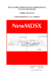
The plot comes up in a separate window, and looks like this:
23
Primer on Matlab
Frank M. Kelso
Figure 1: Full Period Sine Wave
Summary of the example thus far
There are several things you should learn from this example. First let’s review the Matlab
commands I entered to create the sine wave plot.
EDU» delta = (2*pi)/10
delta =
0.5712
EDU» time = [0,delta,2*delta,3*delta,4*delta,...
5*delta,6*delta,7*delta,8*delta,9*delta,10*delta]
time =
Columns 1 through 7
0
0.6283
1.2566
Columns 8 through 11
4.3982
5.0265
1.8850
5.6549
2.5133
3.1416
3.7699
6.2832
EDU» sinewave = sin(time)
sinewave =
Columns 1 through 7
0 0.5878
0.9511
Columns 8 through 11
-0.9511
-0.9511
-0.5878
0.9511
-0.0000
EDU» plot(time,sinewave,'o'
24
0.5878
0.0000
-0.5878
Primer on Matlab
Frank M. Kelso
First, you can create an array in Matlab easily and directly by enclosing a set of values
between square brackets. These values can be separated either by commas (as in the
example above) or by spaces. Also, continuation from one line to the next is
accomplished by three dots at the end of a line (…) to indicate continuation. I had to do
this to enter all eleven values for the time array.
Matlab treats arrays the same as scalars. If I want to take the sine of 0.5, then I would
write, sin(0.5). If I want to take the sine of an array of values (such as the time array)
then I would write sin(time). Notice that I didn’t have to define the sinewave array
or dimension it or allocate memory for it, as I might have had to in another programming
language such as C or Fortran. By typing in
sinewave = sin(time)
Matlab simply created another array called sinewave that had the same dimensions as
the time array, and calculated its values element by element.
Finally, Matlab has a very useful plot command that does all the scaling and gridding for
you. Your only responsibility is to supply it with an x array and a y array of equal size.
Example, continued: Plotting just the first quarter of the sine wave
Continuing our example, let’s suppose we’re only interested in the first quarter of the sine
wave, the rise from 0 to 1. The Matlab code to do this is shown below.
EDU» time = time/4
time =
Columns 1 through 7
0
0.1571
0.3142
0.4712
1.4137
1.5708
EDU» sinewave=sin(time)
sinewave =
Columns 1 through 7
0
0.1564
0.3090
0.4540
Columns 8 through 11
1.0996
1.2566
25
0.6283
0.7854
0.9425
0.5878
0.7071
0.8090
Primer on Matlab
Frank M. Kelso
Columns 8 through 11
0.8910
0.9511
0.9877
1.0000
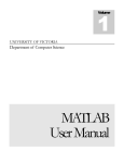
EDU» plot(time,sinewave,'o')
The resultant plot is shown below.
Figure 2: Quarter Period Sine Wave
Once again, notice how simple it is to operate on an entire array of values. If time was a
scalar value, I can divide it by 4 just by writing time/4. If time is an array of values,
then I can divide each value by 4 the same way, just by writing time/4.
Stress Calculation Example, Revisited
Earlier, we created a script file (shown again below) to calculate the normal stress in a
solid round rod when an axial load of P pounds was applied.
EDU>> type stresscalc
% stresscalc.m
script file for calculating stress
P = 1000;
dia = 1;
area = (pi*dia^2)/4;
stress = P/area
26
Primer on Matlab
Frank M. Kelso
EDU>>
We used this program to calculate the stress in a 1” DIA rod.
EDU» stresscalc
stress =
1273.24
EDU»
Suppose we have rods of 5 different diameters in stock (0.5, 0.75, 1.0, 1.25, and 1.50),
and we want to calculate the corresponding stress for each of the 5 diameters. We could
do this by making 5 copies of stresscalc.m, each with a different value assigned to the
variable dia. That’s pretty labor-intensive.
An alternative is to make the variable dia an array containing the values 0.5, 0.75, 1.0,
1.25, and 1.50. We can do this from the Matlab prompt as follows:
EDU» dia = [0.5 0.75 1.0 1.25 1.5]
dia =
0.50
0.75
1.00
1.25
1.50
Remember, I can use either spaces or commas as separators when I’m constructing an
array.
You can think of an array as a subscripted variable. Instead of having just one diameter
dia, we can have 5 diameters d1, d2, d3, d4, and d5 by making the variable dia an array.
That’s what I’ve done with the variable dia, above. Using square brackets tells Matlab
that the variable dia has 5 values, dia (1), dia (2), dia (3), dia (4), and dia (5). I’ll
illustrate this by accessing a few individual array elements (below)2.
EDU» dia(1)
ans =
2
C-programmers will need to be careful! Matlab calls the first element in an array “element #1”, not
“element #0”.
27
Primer on Matlab
Frank M. Kelso
0.50
EDU» dia(3)
ans =
1.00
EDU»
Now let’s modify stresscalc.m, make dia an array, and calculate the corresponding
stresses for each diameter.
I’ll make the changes to stresscalc.m using Matlab’s m-file editor, which I can start
up with the following command,
EDU» edit stresscalc.m
This command brings up the “edit” window, and the edit window contains my
stresscalc.m file. It’s just as easy (perhaps easier) than mousing over to the
File…open menu option. Either way works! I’m now in my text editor, and ready to
make the changes to stresscalc.m.
Matlab Editor Window
After making my changes and putting away the text editor, I’m back in the command
window.
28
Primer on Matlab
Frank M. Kelso
I’ll quickly review the changes I just made by typing out the file from inside the
command window.
EDU» type stresscalc.m
% stresscalc.m
Calculates the stress in a rod
P = 1000;
dia = [0.5 0.75 1.0 1.25 1.50];
area = (pi*dia^2)/4;
stress = P/area
Now we can run the modified stresscalc.m, and have a single program calculate
stress for all 5 diameters! This is demonstrated below.
EDU» stresscalc
??? Error using ==> ^
Matrix must be square.
Error in ==> C:\Matlab_SE_5.3\work\stresscalc.m
On line 5 ==> area = (pi*dia^2)/4;
EDU»
Wasn’t that easy! Oops: maybe not so easy after all. It appears I made a mistake: Matlab
is complaining about line 5 of my stresscalc.m program. It’s telling me that it ran into
a problem using “^” (exponentiation). The problem seems to be that exponentiation
doesn’t work on anything but a square matrix. ?? What’s all that about?
We seem to have hit a snag
Our program didn’t work, and the error message we’re getting isn’t making a whole lot of
sense (yet!) The problem appeared when we converted dia from a scalar to an array. It
would appear that exponentiation works for scalars, but doesn’t work for arrays. Matlab
identified line 5 as the offending line of code:
area = (pi*dia^2)/4;
A careful reading of the (rather cryptic) error message says as much.
29
Primer on Matlab
Frank M. Kelso
??? Error using ==> ^
Matrix must be square.
To really understand why we hit a snag here, we must first understand a little more about
how Matlab thinks of an array3.
arrays and vectors (and matrices)
Matlab represents scalars, vectors and matrices using arrays. The variable dia in the
program above, for example, is a row vector.
A row vector, you’ll recall, is a vector having one horizontal row (and several columns),
while a column vector has one vertical column (and several rows).
(a) row vector
(b) column vector
Figure 3: Row and column vectors
If I wanted to make dia into a column vector instead of a row vector, I could take the
transpose of the row vector using the ’ operator. This is shown in the example below.
EDU» dia = [0.5 0.75 1.0 1.25 1.50]
dia =
0.5000
0.7500
1.0000
1.2500
3
1.5000
We’ll come back and fix our “stresscalc.m” program after we’ve gained some insight into vectors and
matrices, the subject of the next section. Right now let’s put stresscalc on the back shelf and return to it
a little later.
30
Primer on Matlab
Frank M. Kelso
EDU» dia = dia'
dia =
0.5000
0.7500
1.0000
1.2500
1.5000
EDU»
I changed the dia variable from a row vector to a column vector using the transpose
operator. I can change it back from a column vector to a row vector just as easily using
the transpose operator again.
EDU» dia = dia'
dia =
0.5000
0.7500
1.0000
1.2500
1.5000
EDU»
I can enter column vectors as easily as row vectors by using the semi-colon (;) separator.
A semi-colon basically says to Matlab, “end of that row!”. For example, suppose I want
to create a second column vector of possible diameters. I can create that vector and enter
its values as follows:
EDU» dia2 = [1.75; 2.0; 2.25; 2.50; 2.75]
dia2 =
1.7500
2.0000
2.2500
2.5000
2.7500
EDU»
I can access individual elements of a column vector as easily as I did a row vector. The
third element of the column vector, for example, is accessed as
31
Primer on Matlab
Frank M. Kelso
EDU» dia2(3)
ans =
2.2500
EDU»
A matrix is an array of multiple rows and columns, and it is entered just as you might
expect:
EDU» mat1 = [1 2 3; 4 5 6; 7 8 9]
mat1 =
1
2
3
4
5
6
7
8
9
Here I’ve created a matrix mat1 and entered it row by row.
Individual elements of a matrix can be accessed by referring to the row and column
numbers of a particular element. For example, the element at row 3 column 2 of the
matrix mat1 can be accessed by
EDU» mat1(3,2)
ans =
8
Operations can be performed on matrices, just as with scalars or vectors. I can create a
new matrix, mat2, by squaring mat1.
EDU» mat2 = mat1^2
mat2 =
30
66
102
36
81
126
42
96
150
EDU»
Remember that squaring the matrix mat1 is the same as mat1*mat1, and must follow
the rules of matrix multiplication4.
4
If two matrices A and B are multiplied together to produce a matrix C, then element i,j of the product
matrix is equal to the product of row i of matrix A and column j of matrix B. That is, Cij = $Ain Bnj
32
Primer on Matlab
Frank M. Kelso
I can also multiply a row vector times a column vector, as shown in the example below. I
have a row vector, dia:
EDU» dia
dia =
0.5000
0.7500
1.0000
1.2500
1.5000
and I have a column vector, dia2
EDU» dia2
dia2 =
1.7500
2.0000
2.2500
2.5000
2.7500
Vector multiplication is defined as taking each element of the row vector and multiplying
by the corresponding element in the column vector, and summing the individual products.
For this example, the result of the row vector dia times the column vector dia2 will be
calculated as follows:
0.5*1.75 + 0.75*2.0 + 1.0*2.25 + 1.25*2.50 + 1.5*2.75
This operation is called the inner product of the row vector and the column vector, and it
results in a single scalar value (11.875, in this example).
I’ll do that same calculation in Matlab, and store the result into a new variable, dia3.
EDU» dia3 = dia * dia2
dia3 =
11.8750
EDU»
33
Primer on Matlab
Frank M. Kelso
I am assuming that you the reader are already familiar with the rules of vector and matrix
multiplication, and so I won’t go over them further5.
According to the rules of vector multiplication, I cannot multiply a row vector by a row
vector – that is an illegal (undefined) matrix operation because there aren’t enough
columns to form the inner product. This is demonstrated below.
EDU» dia4 = dia * dia
??? Error using ==> *
Inner matrix dimensions must agree.
EDU»
That explains the error in my stress calculation program. In attempting to compute the
area corresponding to each diameter, I attempted an illegal matrix multiplication (row
vector squared, which is the same as row vector times row vector). I can demonstrate that
error easily enough in the code fragment below.
EDU» dia
dia =
0.5000
0.7500
1.0000
1.2500
1.5000
EDU» area = (pi*dia^2)/4
??? Error using ==> ^
Matrix must be square.
EDU»
When I squared the diameter dia (i.e. dia^2), I was attempting to square a row vector,
which is the same as dia * dia. And that’s not a valid matrix operation.
Fortunately, I can use the dot operator to perform the “square” operation element by
element.
EDU» area = (pi*dia.^2)/4
area =
0.1963
0.4418
0.7854
1.2272
1.7671
EDU»
5
.If you aren’t comfortable with matrix operations, now would be a good time to review a text on linear
algebra. Matlab is after all an abbreviation for Matrix Laboratory.
34
Primer on Matlab
Frank M. Kelso
If you look closely at the example above, you’ll notice a period (a “dot”) between dia
and ^2. This dot tells Matlab to ignore conventional matrix operations and operate
element by element instead.
Another example might help illustrate this point.
If I have two matrices, mat1 and mat2, I can matrix multiply them together if their sizes
match up.
First I’ll create two matrices of the same size
EDU» mat1 = [1 2 3;4 5 6;7 8
mat1 =
1
2
3
4
5
6
7
8
9
9]
EDU» mat2 = mat1 + 1
mat2 =
2
3
4
5
6
7
8
9
10
Next I’ll multiply them together, without the dot operator. Matlab will use the rules of
matrix multiplication to calculate the result (mat3).
EDU» mat3 = mat1*mat2
mat3 =
36
42
48
81
96
111
126
150
174
EDU»
I can also multiply them together element by element using the dot operator.
EDU» mat3 = mat1.*mat2
mat3 =
2
6
12
20
30
42
56
72
90
EDU»
35
Primer on Matlab
Frank M. Kelso
This is a completely different matrix multiplication (using the dot operator) from the
previous example (without using the dot operator), with a completely different result.
Compare the two results to make sure you understand the difference!
Here’s another example. I can cube mat1 using matrix multiplication, or I can cube it
element by element using the dot operator, as shown in the example below.
EDU» mat3 = mat1^3
mat3 =
468
576
1062
1656
684
1305
2034
1548
2412
EDU» mat3 = mat1.^3
mat3 =
1
8
27
64
125
216
343
512
729
EDU»
The dot operator is invoked by preceding the operator with a dot, i.e. mat3.*2 or
mat3.^2. Inserting the dot changes the operator from matrix operations to element by
element operations.
This concludes our brief introduction to vectors and matrices. This is an important Matlab
topic, and we’ll certainly come back to it in much greater detail a little later on. But right
now we have some unfinished business. With our new understanding of how Matlab
handles vectors and matrices – in particular the difference between matrix operators and
“element by element” operators - we are now in a position to go back and fix the errors in
the stresscalc example program.
Fixing our stress calculation example program
In our stress calculation example, we had an array of rod diameters and wanted to
calculate the normal stress in each rod when it is loaded by an axial load P of 1000 lbs.
The stresscalc.m program tried to do this:
36
Primer on Matlab
Frank M. Kelso
EDU» type stresscalc.m
% stresscalc.m
Calculates the stress in a rod
P = 1000;
dia = [0.5 0.75 1.0 1.25 1.50];
area = (pi*dia^2)/4;
stress = P/area
But when we tried to run it, we got an error message:
EDU» stresscalc
??? Error using ==> ^
Matrix must be square.
Error in ==> C:\Matlab_SE_5.3\work\stresscalc.m
On line 5 ==> area = (pi*dia^2)/4;
EDU»
We ran into this error because matrix multiplication (row vector times row vector, or in
this case area^2=area*area) is illegal.
What we really want to do is operate element by element, which we can do using the dot
operator6. The corrected code is shown below. Notice I made P a row vector so that I
could divide P by area, element by element. I use the dot operator to calculate area (the
dot between dia and ^2) and also to do the division of row vector P by row vector area
(the dot between P and /).
EDU» type stresscalc.m
% stresscalc.m
Calculates the stress in a rod
P = [1000 1000 1000 1000 1000];
dia = [0.5 0.75 1.0 1.25 1.50];
area = (pi*dia.^2)/4;
stress = P./area
Let’s try running it again and see if we have fixed the error.
EDU» stresscalc
stress =
1.0e+003 *
5.0930
2.2635
6
1.2732
0.8149
0.5659
Refer to the discussion in the preceding section for information on the dot operator.
37
Primer on Matlab
Frank M. Kelso
EDU»
The result is row vector of stress values. We now have a working stress calculation
program.
38
Primer on Matlab
Frank M. Kelso
Part II: Basics of Matlab Programming
Working through Part I of this primer provided a general understanding of Matlab’s
capabilities as an equation solver. We wrote some very simple programs, gaining some
familiarity with how to formulate equations in a format that Matlab can work with.
We now shift our focus to programming. As with most programming languages, Matlab
supports structured programming (main programs and callable functions, scoping, data
structures), conditionals (if statements), and iteration (for and while loops). We will
investigate each of these in turn, but we’ll begin with more information on matrices.
Table of Contents (Part II)
More About Vectors and Matrices
Creating vectors and matrices
Colon constructor
Linspace and logspace commands
Some useful commands for working with vectors and matrices
Function m-files
“Declaring” the function and passing in information
More about the function declaration line
Matlab Help and the function m-file
“If” Statements
Relational operators
elseif statements
Exercises: conditionals
Looping
for loops
while loops
Input and Output
39
Primer on Matlab
Frank M. Kelso
More About Vectors and Matrices
Vectors and matrices are the basic building blocks we work with in Matlab. This section
provides a better understanding of some of the more useful Matlab commands for
creating and manipulating them.
Creating vectors and matrices using direct construction
We’ve already looked at one method of creating vectors and matrices: direct
construction. Using direct construction to create a row vector dia, for example, we
would write
EDU» dia = [0.5 0.75 1.0 1.25 1.5]
dia =
0.5000
0.7500
1.0000
1.2500
1.5000
EDU»
Individual elements in the vector may be separated by either spaces or commas.
Using direct construction to create a 3x3 matrix, for example, we would write
EDU» a = [1 2 3; 4 5 6; 7 8 9]
a =
1
2
3
4
5
6
7
8
9
EDU»
Individual rows are separated by semi-colons or “carriage returns,” as demonstrated
below.
EDU» b = [2 3 4
5 6 7
8 9 10]
b =
2
5
8
3
6
9
4
7
10
EDU»
40
Primer on Matlab
Frank M. Kelso
Direct construction works nicely, as long as there are not too many elements. Suppose,
for example, you wanted to create a row vector of all the integer numbers between 1 and
100. Typing in all 100 integers would be arduous (and boring), so Matlab has other
methods of constructing a vector (or a matrix). The first method we’ll look at is called the
colon constructor.
colon constructor
To construct a row vector of all integer numbers between 1 and 100, use the colon
operator as follows:
EDU» numbers=1:100;
EDU»
I suppressed the output with a semi-colon, for obvious reasons. Here, Matlab fills in all of
the integers between 1 and 100 (inclusive) and assigns them to the variable numbers. If
we wanted just the odd numbers between 1 and 10 (e.g. 1, 3, 5, 7, and 9) we would type
EDU» numbers=1:2:9
numbers =
1
3
5
7
9
EDU»
The format for the colon constructor is start:increment:stop. Leaving out the increment
causes Matlab to default to integral numbers (that is, a step size of 1).
Can you figure out the contents of the values vector after the following assignment
statement?
EDU» values=0.1:0.5
Try it and see if you’re are correct!
41
Primer on Matlab
Frank M. Kelso
Exercise
Create an array from 0 to pi in steps of 0.1*pi using colon construction.
Solution
EDU» angle = (0:0.1:1.0)*pi
angle =
Columns 1 through 7
0
0.3142
0.6283
Columns 8 through 11
2.1991
2.5133
0.9425
2.8274
1.2566
1.5708
1.8850
3.1416
EDU»
The code in the parentheses (0:0.1:1.0) constructs a row vector that starts at zero and goes
up in increments of 0.1 to a final value of 1.0. The result is
[0 0.1 0.2 0.3 0.4 0.5 0.6 0.7 0.8 0.9 1.0]
By enclosing it in parentheses and multiplying by pi, we get a vector that starts at zero
and goes up to a value of pi in steps of 0.1*pi.
Linspace command
A third method for constructing a row vector is the linspace command. Checking the
help text for the linspace function results in
EDU» help linspace
LINSPACE Linearly spaced vector.
LINSPACE(x1, x2) generates a row vector of 100 linearly
equally spaced points between x1 and x2.
LINSPACE(x1, x2, N) generates N points between x1 and x2.
See also LOGSPACE, :.
EDU»
Let’s illustrate the use of linspace with an example. Suppose I wanted an 11-element
vector between zero and pi. I can create it using linspace as follows:
42
Primer on Matlab
Frank M. Kelso
EDU» time = linspace(0,pi,11)
time =
Columns 1 through 7
0
0.3142
0.6283
Columns 8 through 11
2.1991
2.5133
2.8274
0.9425
1.2566
1.5708
1.8850
3.1416
EDU»
The advantage of linspace over the colon constructor is that I can specify the number
of points I want to have filled in between the start and the end point: linspace will
figure out the appropriate increment.
Creating matrices
Matlab provides some very useful commands for creating “standard” matrices that can be
used instead of the direct construction method discussed earlier. To create a 2 x 3 matrix
filled with ones, for example;
EDU» a = ones(2,3)
a =
1
1
1
1
1
1
EDU»
creates a matrix with 2 rows and 3 columns of ones.
To create a square 4 x 4 matrix,
EDU» a = ones(4)
a =
1
1
1
1
1
1
1
1
1
1
1
1
1
1
1
1
EDU»
If only one argument is provided, Matlab assumes the matrix is square.
43
Primer on Matlab
Frank M. Kelso
Matlab also provides a zeros command in case the matrix should be loaded with zeros
rather than ones.
EDU» a = zeros(4)
a =
0
0
0
0
0
0
0
0
0
0
0
0
0
0
0
0
EDU»
The eye command is used to construct an identity matrix, as shown below.
EDU» a = eye(3)
a =
1
0
0
1
0
0
0
0
1
EDU»
The command you choose to use will of course depend on the task at hand.
Some useful commands for working with vectors and matrices
The basic building block in Matlab is the matrix, and Matlab provides many useful
commands for working with them.
The size of a vector or matrix is often a useful thing to know. There are two functions for
determining size:
[r,c] = size(mat)
returns a row vector [row col] specifying the dimensions
of the matrix mat.
len = length(mat)
returns a scalar (in this case, len) containing the maximum
dimension of the matrix mat.
Lets look at some examples to clarify the use of these Matlab commands.
44
Primer on Matlab
Frank M. Kelso
Suppose we’re working again with the stresscalc program, which looks like this:
EDU» type stresscalc.m
% stresscalc.m
Calculates the stress in a rod
P = [1000 1000 1000 1000 1000];
dia = [0.5 0.75 1.0 1.25 1.50];
area = (pi*dia.^2)/4;
stress = P./area
Running the program from the command window results in the following stress
calculations:
EDU» stresscalc
stress =
1.0e+003 *
5.0930
2.2635
1.2732
0.8149
0.5659
EDU»
Because I ran the script from the Matlab interpreter, all of the script file variables are in
the Matlab workspace, and I have access to them from the Matlab command window. I
can look at stresscalc’s P variable, for example, by typing in
EDU» P
P =
1000
1000
1000
1000
1000
EDU»
I can check on the length of the row vector P as follows:
EDU» length(P)
ans =
5
EDU»
Both the size and length commands will work on vectors as well as matrices, because a
vector is a specific kind of matrix – that is, a matrix with just one row (and several
columns). This is demonstrated by the size command, which will return the number of
rows and columns in the matrix.
45
Primer on Matlab
Frank M. Kelso
EDU» size(P)
ans =
1
5
EDU»
Here we see that the row vector P has one row, and five columns.
Question: Will size and length work on a scalar as well as a vector or a matrix?
Answer: Yes: Matlab considers scalars and vectors to be special kinds of matrices,
and treats them all as such. This is demonstrated below in checking in the
size of the scalar pi and the scalar 4.
EDU» size(pi)
ans =
1
1
EDU» size(4)
ans =
1
1
EDU»
These are all considered matrices by Matlab, which provides a consistent and uniform
means of working with every type of numerical quantity, vector, scalar or n x m matrix.
Matlab also provides a lot of very useful matrix operations, some of which are shown
below.
det(A)
calculate the determinant of the matrix A
inv(A)
calculate the inverse of the matrix A
inverse division
calculate the inverse and perform the matrix multiplication
These are best illustrated using a specific example.
Example: Solving a system of equations
46
Primer on Matlab
Frank M. Kelso
Suppose you wanted to solve the following set of 3 equations and 3 unknowns:
3x1 + 2x2 + 5x3 = 15
x1 – 3x2 + 8x3 = -20
4x1 + 5x2 – 7x3 = 14
This can be represented in matrix format as the matrix equation
Ax = b
Where A is a 3x3 matrix, and both x and b are 3x1 column vectors, as shown below.
5 º ªx1 º
ª3 2
«1 3 8 » ˜ « x »
«
» « 2»
«¬ 4 5 7 »¼ «¬ x 3 »¼
ª 15 º
« 20»
«
»
«¬ 14 »¼
This equation can be solved for the unknown x by first calculating the inverse of A,
designated A–1. Remember that, by definition,
A–1 A = I
Where I is the identity matrix. Once we have determined A–1, we can pre-multiply both
sides of the matrix equation by A–1 and get
A–1 A x = A–1 b
x = A–1 b
Which is the solution for x.
This solution procedure only works, however, when A is a well-conditioned matrix.
Remember – some matrices are singular, which means they have no inverse. If a matrix is
47
Primer on Matlab
Frank M. Kelso
singular, then its determinant will be equal to zero. Likewise, if a matrix is illconditioned, then its determinant will be near zero.
Let’s solve this matrix equation using Matlab.
The first step will be to create the matrix A and the column vector b, as follows.
EDU» A = [3 2 5
1 -3 8
4 5 -7]
A =
3
2
5
1
-3
8
4
5
-7
EDU» b = [15; -20; 14]
b =
15
-20
14
Next, we’ll check the determinant of A to make sure our solution procedure is valid.
EDU» det_A = det(A)
det_A =
106
EDU»
Since the determinant is nowhere near zero, it has an inverse and we can proceed with the
solution. Taking the inverse of A
EDU» A_inverse = inv(A)
A_inverse =
-0.1792
0.3679
0.2925
0.3679
-0.3868
-0.1792
0.1604
-0.0660
-0.1038
EDU»
And multiplying it by the column vector b gives us the column vector x.
EDU» x = A_inverse*b
x =
-5.9528
10.7453
48
Primer on Matlab
Frank M. Kelso
2.2736
EDU»
Our solution, then, is
x1 = -5.9528
x2 = 10.7453
x3 = 2.2736
We could also have solved this matrix equation using inverse division, as shown below.
EDU» x = A\b
x =
-5.9528
10.7453
2.2736
EDU»
When do you use inverse division?
Calculating a matrix inverse A-1 can be computationally expensive. When that is the case,
it is better to calculate the inverse once, and use it over and over on different solution
vectors b.
This isn't always the case: many times there is only one matrix equation to solve, and one
solution vector to compute. With only one solution to compute, inverse division makes
sense because it's simple and straightforward to write.
49
Primer on Matlab
Frank M. Kelso
Function M-Files
There are two types of m-files: script m-files and function m-files.
M-file Categories
A script m-file such as stresscalc.m can be thought of as a main program, while a
function m-file can be thought of as a callable function (sub-program). We’ve already
discussed script m-files in Part I. An example of such a file is our stress calculation file,
shown below.
EDU» type stresscalc.m
% stresscalc.m
Calculates the stress in a rod
P = [1000 1000 1000 1000 1000];
dia = [0.5 0.75 1.0 1.25 1.50];
area = (pi*dia.^2)/4;
stress = P./area
A function m-file allows you to implement a callable function. Suppose, for example, we
want to modify stresscalc by having it call a function to compute the cross-sectional
area. Let’s create a function called “roundarea”. I pass in an array of diameters, and it
passes back an array of the corresponding cross-sectional areas.
I’ll create a new file called “roundarea.m” using the Matlab editor7. After creating the
text file, closing the editor and returning to the command window, I’ll verify my new
creation by listing it, as follows.
7
The easiest way to create a new file is using the “File…New” command from the command window
menu bar. If the file already existed, we could simply have typed “edit roundarea.m” from the EDU>>
50
Primer on Matlab
Frank M. Kelso
EDU» type roundarea.m
function a = roundarea(dia)
% ROUNDAREA calculate the cross-sectional area of a circle
a = (pi*dia.^2)/4;
EDU»
We’ll discuss this new file a little later – right now I want you to see it in action. I
modified my stresscalc program to call this new function roundarea, as follows:
EDU» type stresscalc.m
% stresscalc.m
Calculates the stress in a rod
P = [1000 1000 1000 1000 1000];
dia = [0.5 0.75 1.0 1.25 1.50];
%area = (pi*dia.^2)/4;
area = roundarea(dia);
stress = P./area
Notice that I’ve commented out the original area calculation (using the “%” symbol) and
replaced it with a call to function roundarea. I’ll run the modified stresscalc
program to demonstrate that it produces the exact same results.
EDU» stresscalc
stress =
1.0e+003 *
5.0930
2.2635
1.2732
0.8149
0.5659
EDU»
Matlab implements most of its own functions in the same way. The Matlab “angle”
function, for example, was discussed in the complex numbers section of this document. If
we take a closer look at angle.m, we see that it is a function m-file:
EDU» type angle.m
function p = angle(h)
%ANGLE Phase angle.
%
ANGLE(H) returns the phase angles, in radians, of a matrix
%
with complex elements.
prompt in the command window. Since the file doesn’t exist yet, though, Matlab would be unable to locate
an existing roundarea.m file and would report it as an error.
51
Primer on Matlab
Frank M. Kelso
%
%
See also ABS, UNWRAP.
%
%
Copyright (c) 1984-98 by The MathWorks, Inc.
$Revision: 5.3 $ $Date: 1997/11/21 23:28:04 $
% Clever way:
% p = imag(log(h));
% Way we'll do it:
p = atan2(imag(h), real(h));
EDU»
Function m-files allow us to break our program down into smaller, more manageable
subprograms: a very useful concept!
“Declaring” the function and passing in information
The first line of any function m-file is the function declaration. From our roundarea
example, the function declaration looks like this:
function a = roundarea(dia)
Values are passed in to a function through the input argument list. Here we are only
passing in a single variable, dia. Matlab uses the “pass by value” convention when
passing information into a function. This means that if the value of dia is changed inside
the function, that change is not reflected in the calling program. This is a very important
point, illustrated in the example program below.
EDU» type test.m
% program test
%
% this program checks to see if the value of the variable "dia"
% can be altered by the function changedia.
%
dia = 1.0;
% assign a value to dia
changedia( dia );
% change the value inside changedia
dia
% no semi-colon: print out the value of dia
EDU»
The function changedia is listed below.
52
Primer on Matlab
Frank M. Kelso
EDU» type changedia.m
function changedia( dia )
% CHANGEDIA: change the value of the input variable dia
%
and see if the calling program is aware
%
of the change.
dia = 2.0;
EDU»
What would you expect Matlab to print out when it gets to the last line of the main
program and displays the value if dia? Will it be 1.0 or 2.0? Let’s run the program and
see.
EDU» test
dia =
1
EDU»
The value is 1.0, not 2.0, because changes made to the input parameter(s) inside the
function are not passed back to the calling program. Information travels through the input
variables in one direction only, from the calling function to the called function – not the
other way around.
More about the function declaration line
The function declaration is the first line of a function m-file. It declares the name of the
function, and Matlab expects the name of the file to match the name of the function. If I
write the function roundarea, for example, then it must be stored in a file named
roundarea.m.
The function declaration begins with the keyword function. As we have seen,
parameters can be passed in to the function by enclosing the parameter names in
parentheses. If a parameter value is to be passed back to the caller, then the function
declaration line will also declare the output variables. This is illustrated by
stresscalc’s use of the function roundarea. Here the program stresscalc passes
53
Primer on Matlab
Frank M. Kelso
in the diameter of a circle (dia) to the roundarea function, and gets back the
corresponding cross sectional area of the circle (assigned to the variable area). The line
of code where all this occurs is bolded in the listing below.
% stresscalc.m
Calculates the stress in a rod
P = [1000 1000 1000 1000 1000];
dia = [0.5 0.75 1.0 1.25 1.50];
area = roundarea(dia);
stress = P./area
The value of the cross sectional area is calculated inside of the roundarea function, and
returned. The output variable is declared in the function declaration, as shown below.
function a = roundarea(dia)
% ROUNDAREA calculate the cross-sectional area of a circle
a = (pi*dia.^2)/4;
Here the value of the output variable “a” is assigned as the value of roundarea, and
returned to the calling program. The actual value of “a” is calculated in the body of the
function.
Matlab Help and the function m-file
Matlab has a very simple method for implementing its help function. When you ask
Matlab for help on a particular function (such as help angle, or help atan2), it first
finds the m-file that implements the function you’re interested in. It then reads in the
initial comment lines, and prints them out. The Matlab convention is to make the initial
comment lines of an m-file appropriate for providing help to a user.
The roundarea.m file, for example, begins with a single comment line below the
function declaration statement (as shown below).
function a = roundarea(dia)
% ROUNDAREA calculate the cross-sectional area of a circle
a = (pi*dia.^2)/4;
54
Primer on Matlab
Frank M. Kelso
When I type “help roundarea” at the command prompt, the following message is
printed out in the command window:
EDU» help roundarea
ROUNDAREA calculate the cross-sectional area of a circle
EDU»
Matlab found my function m-file roundarea.m and then listed all of the comment lines
after the function declaration statement and before the first executable statement.
If Statements (Conditionals)
“If statements” are used to evaluate different conditions and execute the appropriate
portion of code. For example, suppose we write a function that calculates the cross
sectional area for both hollow tubes as well as rectangular barstock. Let’s create a
function named crossx. Using “File…New” I’ll create a file named crossx.m as
shown below. (Remember that the name of the m-file should match the name of the
program or function. Refer to the section on function m-files for more information.)
Figure: Creating a New Function m-file Named crossx.m
55
Primer on Matlab
Frank M. Kelso
Our new function crossx will accept three input parameters. The first input parameter,
shape, is a string that is set to either ‘tube’ or ‘rect’. The second and third parameters are
the two characteristic dimensions of the shape. If the shape is a hollow tube, then dim1 is
the outer diameter and dim2 is the inner diameter. If the shape is rectangular, then dim1
is the width and dim2 is the thickness.
We’ll use an if statement to determine the shape and calculate the cross sectional area
using the appropriate formula. The function m-file is shown below.
function
% CROSSX
%
%
a = crossx(shape,dim1,dim2)
calculate the cross-sectional area of the shape.
Works with either hollow tube shapes (shape='tube')
or rectangular shapes (shape='rect').
if (shape=='tube')
a = (pi*(dim1^2-dim2^2))/4;
else
a = dim1*dim2;
end
If the expression shape == ‘tube’ evaluates to TRUE, then the subsequent area
calculation is executed. If it evaluates to FALSE, however, the program assumes that the
shape is rectangular, and calculates the area “a” as dim1*dim2.
Let’s check and see if this function is working correctly. We can do that with some test
cases right from the command prompt, as follows.
EDU» crossx('tube',1,1)
ans =
0
EDU» crossx('rect',1,1)
ans =
1
EDU» crossx('tube',1,0)
ans =
0.7854
EDU»
56
Primer on Matlab
Frank M. Kelso
The general format of a conditional statement is
if expression
set of matlab statements
else
alternate set of matlab statements
end
Relational Operators
To determine if the shape was a rectangle, the previous example used the logical
expression
if (shape=='tube')
A logical expression (such as shape == ‘tube’) is one that is either TRUE or FALSE.
Matlab knew this was a logical expression because the expression involved a comparison
of shape to ‘tube’.
Did you notice the use of the “double-equals” sign, “==” ? A “single equal” sign = is an
assignment statement, and would have assigned the value ‘tube’ to the variable shape. A
double-equal sign, however, tests to see if the variable shape has a value equal to
‘tube’. If it does, then the entire expression is evaluated and set to TRUE and the if
statement reads, in effect,
if (TRUE)
a = (pi*(dim1^2-dim2^2))/4;
and the subsequent statement (the area calculation for tubes,
a = (pi*(dim1^2-dim2^2))/4 )
is executed accordingly. If shape does not have a value equal to ’tube’, the logical
expression evaluates to FALSE and the subsequent calculation is skipped.
A logical expression involves a comparison of two things, and the comparison takes on a
value of either TRUE or FALSE. Comparisons are accomplished using relational
operators such as the “double-equals” sign, ==. Can you think of some other relational
57
Primer on Matlab
Frank M. Kelso
operators that you would expect Matlab to provide in order to compare one thing to
another?
Matlab provides the following relational operators:
==
<
>
<=
>=
~=
equals
less than
greater than
less than or equal to
greater than or equal to
not equal to
elseif statements
An if-else statement is useful when dealing with two or more possible outcomes (e.g.
“tube” and “rect”). But suppose now we wanted to expand our crossx function (from
the previous example) to handle more than two shapes. To cope with more than two
possible outcomes we could make good use of the elseif statement within our
conditional. The general form of an if statement is
if expression
set of matlab statements
elseif expression
alternate set of matlab statements
elseif expression
alternate set of matlab statements
elseif expression
alternate set of matlab statements
elseif expression
alternate set of matlab statements
else
alternate set of matlab statements
end
(Note: the final “else” statement shown above is optional.)
Let’s illustrate the use of an elseif statement with an example by fixing a flaw in our
crossx function. Right now if a calling program calls crossx with some shape other than
than ‘tube’, the program makes a leap of faith and assumes that the caller wants a
58
Primer on Matlab
Frank M. Kelso
rectangular area calculated. Bad assumption! Here is the current version of the (flawed)
if-statement:
if (shape=='tube')
a = (pi*(dim1^2-dim2^2))/4;
else
a = dim1*dim2;
end
If the calling program assumed that a triangular shape was implemented in crossx, it
might call crossx as follows:
EDU» crossx('tria',2,1)
The calling program is requesting the area of a triangle with a base of 2 inches and a
height of 1 inch. The crossx function incorrectly calculates the area of the triangle as if
it were a rectangle (2 x 1 square inches) and passes the incorrect value back to the caller.
What should crossx have done?
At the very least, it should detect the fact that the caller was requesting a shape that it is
not prepared to calculate, and display an error message. We can implement this response
using an elseif statement, as follows.
function
% CROSSX
%
%
a = crossx(shape,dim1,dim2)
calculate the cross-sectional area of the shape.
Works with either hollow tube shapes (shape='tube')
or rectangular shapes (shape='rect').
if (shape=='tube')
a = (pi*(dim1^2-dim2^2))/4;
elseif (shape=='rect')
a = dim1*dim2;
else
disp('ERROR: CROSSX.M: unrecognized shape.')
a = 0;
end
59
Primer on Matlab
Frank M. Kelso
Now our crossx function is a little more “bulletproof 8.” The function now makes sure
that the shape is one that it is equipped to deal with (either tube or rect). If it isn’t, an
error message is displayed using the disp command. disp is a Matlab function that
provides unformatted output, and it is very useful for reporting error messages and
debugging.
disp( displaystring )
types out displaystring in the command window
disp( varname )
types out the value of the variable varname in the
command window
We’ll discuss input–output commands such as disp in a later section.
Exercises: Conditionals
1. Expand the crossx function to handle tubular (‘tube’), rectangular (‘rect’), triangular
(‘tria’), and hollow square(‘squa’) shapes.
2. Did you notice that I used four letter identifiers (e.g. ‘rect’, ‘tube’, etc) in the
preceding exercise? Try calling crossx with something other than a four letter
identifier; for example,
EDU» crossx('triangular',2,1)
You would expect to get the prearranged error message ('ERROR: CROSSX.M:
unrecognized shape.'), from the else statement in crossx, wouldn’t you? In fact,
you would get the following error message:
EDU» crossx('triangular',2,1)
??? Error using ==> ==
8
It is a little more bulletproof, but it needs more work. Make sure to look at exercise 2 of this section to
find and rectify a significant shortcoming of this revised version of the crossx code.
60
Primer on Matlab
Frank M. Kelso
Array dimensions must match for binary array op.
Error in ==> C:\MATLAB_SE_5.3\work\crossx.m
On line 6
==> if (shape=='tube')
Please debug this program so that it doesn’t self-destruct if the caller uses more than four
letters to identify the shape. Hint: use the Matlab help function to investigate the use of
the strcmp function.
61
Primer on Matlab
Frank M. Kelso
Looping
If you are at all familiar with other programming languages (and I’m assuming you are)
then you know how important it is to be able to construct loops. A loop is a set of
executable statements that are repeatedly executed until your termination criteria are
satisfied.
Matlab offers two looping constructs: for loops and while loops. A for loop runs through
a set of statements a specified number of times, and a while loop runs through a set of
statements as long as its termination expression evaluates to FALSE. Each of these
looping constructs is discussed below.
for loops
The general form of the for loop is shown below:
for index = array
statement(s)
end
Suppose, for example, we wanted to calculate the factor of safety for each of 5 rods of
diameter 0.5, 0.75, 1.0, 1.25, and 1.5 inches. The rods experience 1000 lbs load in axial
tension. Each rod is made of 1020 HR steel, with a yield strength Sy of 42 ksi.
One way to solve this problem is to use a for loop to run through each of the 5 cases.
“For” loops work well when there is a specified (rather than an indeterminate) number of
cases to run through. In this problem there are exactly 5 cases to consider, so we’ll use a
for loop from 1 to 5. My solution is shown below.
%
%
%
%
%
%
%
%
%
program safety.m
this program is used to calculate the safety factor
guarding against a static overload for a round bar
loaded in axial tension. The load P is 1000 lbs, and
there are 5 different rod diameters. Results are
plotted as a function of diameter.
Author: FMKelso
Date:
May 31st, 2000
62
Primer on Matlab
Frank M. Kelso
dia = [0.5 0.75 1.0 1.25 1.5];
P = 1000;
Sy = 42000;
% trial rod diameters
% axial load
% yield strength
% calculate the stress and the safety factor for all 5 rods
for index = 1:5
stress(index) = P / ((pi*dia(index)^2)/4);
safety(index) = Sy / stress(index);
end
% plot the results
plot(dia,safety,dia,safety,'o');
There are several inefficiencies in this program… can you find them?
Inefficient or not, though, the program works correctly and produces the following plot:
Static Safety Factor versus Diameter
Let’s review the program.
The program begins by initializing some variables (dia, P, and Sy). The for loop then
iterates through all of the statements between the for and the end, one iteration for every
column in the array.
63
Primer on Matlab
Frank M. Kelso
for index = 1:5
stress(index) = P / ((pi*dia(index)^2)/4);
safety(index) = Sy / stress(index);
end
Here, 1:5 uses Matlab’s “colon construction” method for creating a 5-element array (row
vector) named index. The variable index is now equal to [1 2 3 4 5]. The first time
through, index is set to the first element of the array (i.e. index = index(1) = 1).
The stress is calculated for the first diameter dia(1) and stored as the first element in
the stress array, stress(1). Next, the safety factor is calculated by comparing the
allowable stress Sy to the actual stress for this case, stress(1). The result is stored in
safety(1).
Having executed all the statements for index=1, the for loop goes back to the top of the
loop, sets index to the next column in the array (i.e. index = index(2) = 2). stress(2)
and safety(2) are calculated, and the loop counter is incremented, and so on. This
continues until all the columns in the array have been visited. After stress(5) and
safety(5) have been calculated, there are no more columns to the index array and the
for loop terminates.
The next line of code is
plot(dia,safety,dia,safety,'o');
This plot command actually draws two plots simultaneously on the same coordinate axes
in the same figure window. The first is safety as a function of dia, with a line
connecting all the data points. The second plot is safety as a function of dia, but the
‘o’ specifies that just the data points be marked with a circle. The result is a line
showing the general trend of safety as a function of dia, with the actual data points
marked by a circle.
64
Primer on Matlab
Frank M. Kelso
Is that explanation of the plot command still a little “opaque”? Let me show you what I
mean.
If I change my plot command (the last line in my program) to
plot(dia,safety);
It would generate the following plot:
Safety versus Diameter (Line Only)
Just a line, without any circles marking the actual data points.
If I change my plot command to
plot(dia,safety,'o');
It would generate the following plot.
65
Primer on Matlab
Frank M. Kelso
Safety Factor versus Diameter (Data Points Only)
Just circles marking the data points, without a line in between to help show the general
trend.
What if you want both – lines and circles – on the same plot? One way to do that is the
way I implemented it:
plot(dia,safety,dia,safety,'o');
Try This
Modify the safety factor program as follows:
dia = [0.5 0.75 1.0 1.25 1.5];
P = 1000;
Sy = 42000;
% trial rod diameters
% axial load
% yield strength
% calculate the stress and the safety factor for all 5 rods
for index = dia
stress = P / ((pi*index^2)/4);
safety = Sy / stress;
disp(‘safety factor equals’)
disp(safety)
end
Can you predict the output of the following program? Remember – a for loop will
execute once for each column of the array.
66
Primer on Matlab
Frank M. Kelso
Answer
Running the program produces the following results:
safety factor equals
8.2467
safety factor equals
18.5550
safety factor equals
32.9867
safety factor equals
51.5418
safety factor equals
74.2201
These values are identical to the values calculated in the original example program. As
you can see, the first time through the loop, index is set to the first column of the dia
array, and so it takes on a value of 0.5. The second time through it takes on a value of the
second element of the dia array, and so on, until all the elements in the dia array have
been used. 5 results are printed, corresponding to the 5 elements in the diameter array,
dia.
67