1
EPA Waterscape User Manual Draft Version 6.0, March 2015 EPA Waterscape Tools – Version 1.0 User Manual Table of Contents 1. Getting started ............................................................................................................. 1 1.1 Install the EPA Waterscape Tools ............................................................................ 1 1.2 Open ArcMap and load the EPA Waterscape toolbar ........................................ 3 1.3 Data Requirements .............................................................................................. 4 1.4 Online Help ......................................................................................................... 4 2. Creating a new Waterscape Analysis using existing Data .......................................... 5 2.1 Initialize EPA Waterscape Analysis Environment ............................................. 5 2.2 Create New Analysis........................................................................................... 9 2.3 Generate Initial Subset ...................................................................................... 15 2.4 Generate First Score .......................................................................................... 17 2.5 Generate Second Score ..................................................................................... 25 2.6 Generate Second Subset .................................................................................... 28 2.7 Add back Features............................................................................................. 31 2.8 Generate Report ................................................................................................ 34 2.9 Delete Analysis Step(s) ..................................................................................... 39 2.10 Create Analysis from existing Analysis ............................................................ 40 3. Setting up custom Data ............................................................................................. 42 3.1 Add Properties to Base Analysis Layer ............................................................ 45 1.2 Import Study Area from Base Analysis Layer .................................................. 52 1.3 Set Custom Database as Default EPA Waterscape Administration Database .. 58 2. Configuration ............................................................................................................ 64 2.1 Symbology ........................................................................................................ 64 2.2 Report................................................................................................................ 64 3. Analysis Scenario Examples ..................................................................................... 66 3.1 Massachusetts – Designated Uses ..................................................................... 67 3.2 Ohio – Nutrients ................................................................................................ 69 3.3 Vermont – Protection ........................................................................................ 72 ii EPA Waterscape Tools – Version 1.0 User Manual 1. Getting started 1.1 Install the EPA Waterscape Tools Software Requirements ArcGIS 10.1/10.2.x EPA Waterscape Tools 10.1 for ArcGIS 10.1 or 10.2 for ArcGIS 10.2.x The EPA Waterscape tool is installed by running the setup file EPAWaterscape.msi. Double-click the msi file to launch the installation and click Next in the Welcome window. Figure 1-1 - EPA Waterscape InstallShield Wizard Welcome Window The EPA Waterscape tools are installed by default under C:\Program Files (x86)\ESRI\EPAWaterscape. March 2015 1 EPA Waterscape Tools – Version 1.0 User Manual Modify the default installation location if needed and click Next to complete the installation process. Figure 1-2 – Destination Folder The installation creates 2 directories under the EPAWaterscape folder, Bin and Templates. The Bin directories contains the applications files (.dll) as well as the online help (.chm), configuration file (.xml) and the default supporting file geodatabase (WaterscapeAdmin.gdb). It also contains the subdirectory lyrfiles storing the layer files defining the symbology used by the tools. March 2015 2 EPA Waterscape Tools – Version 1.0 User Manual Figure 1-3 – Bin Directory Contents The Templates directory stores the templates used when generating reports in Microsoft Excel or Word. Figure 1-4 – Templates Directory Contents 1.2 Open ArcMap and load the EPA Waterscape toolbar Open ArcMap. Create a new empty map, and save it as WaterscapeAnalysis.mxd (or any other name). Right click on the menu bar to pop up the context menu showing available tools and select EPA Waterscape. March 2015 3 EPA Waterscape Tools – Version 1.0 User Manual The EPA Waterscape toolbar is shown below. 1.3 Data Requirements The data required to perform the analyses is installed with the application. No additional data is required. If you want to use your own data, refer to section 3.0 Setting up custom data. 1.4 Online Help The online help is available by clicking the Help button on the EPA Waterscape toolbar or in the forms for each function. March 2015 4 EPA Waterscape Tools – Version 1.0 User Manual 2. Creating a new Waterscape Analysis using existing Data The EPA Waterscape tools allow ranking input polygon features using a set of preset properties to identify priority areas for a given purpose. A set of properties characterizing US States are installed with the application and may be used to run analyses. This supporting data is installed in the WaterscapeAdmin.gdb geodatabase located in the installation location\EPAWaterscape\bin folder. 2.1 Initialize EPA Waterscape Analysis Environment In your saved map document, click the EPAWaterscape function on the EPA Waterscape toolbar. The tool copies supporting tables from the default WaterscapeAdmin.gdb geodatabase located in the installation location\EPAWaterscape\bin folder as well as the WSStudyArea feature class into a new geodatabase named after the map document and located in the same directory as the map document. In the picture below, the map document was saved as WaterAnalysis.mxd in the EPAWATERSCAPE\Analyses subdirectory. The tool created a new geodatabase called waterscapeanalysis.gdb as well in the same location. It copies the WSStudyArea feature class defining the study area polygons available for analysis as well as the EPAWaterscape administration tables: WSAnalyses WSAnalysesType WSAnalysisSteps WSProperties WSPropertyAnalysisStep Initially, only the WSProperties and WSAnalysisType tables are populated. The other tables will be populated with the information generated when creating the new analyses. March 2015 5 EPA Waterscape Tools – Version 1.0 User Manual Figure 2-1 – Initial Database The tool adds the WSStudyArea polygon feature class into the Tables of Contents of ArcMap. This layer shows the area where analyses may be performed. The tool also adds the supporting tables for the Waterscape analysis. March 2015 6 EPA Waterscape Tools – Version 1.0 User Manual Figure 2-2 – Initial Data added to the map It opens the EPAWaterscape form that may be docked in the screen. The form does not contain any existing analysis initially. March 2015 7 EPA Waterscape Tools – Version 1.0 User Manual Figure 2-3 – EPAWaterscape Form – First Analysis March 2015 8 EPA Waterscape Tools – Version 1.0 2.2 User Manual Create New Analysis Click the New button to start creating a new analysis. Figure 2-4 – New Button in EPA Waterscape Form The ‘New’ button is renamed ‘Create’. The top section of the form is editable and a title and description for the new analysis may be entered. The Study Area dropdown lists all the available study areas where analyses may be performed. March 2015 9 EPA Waterscape Tools – Version 1.0 User Manual Figure 2-5 - New Analysis – After clicking ‘New’ March 2015 10 EPA Waterscape Tools – Version 1.0 User Manual The Property dropdown lists property groups available for the current selected StudyArea. By default only the group All Properties is available. Additional groups may be created by selecting the New… option in the Properties dropdown list. Figure 2-6 – New… Properties Option After clicking New, a new grouping of properties for the current StudyArea may be created and made available in the main EPAWaterscape form. Figure 2-7 – New Properties Group Window Enter a title and description for the new analysis, select the StudyArea and Properties of interest and click Create. The Create button reverts back to New. March 2015 11 EPA Waterscape Tools – Version 1.0 User Manual Figure 2-8 – New Analysis – After Clicking ‘Create’ The tool copies the supporting data associated with the selected StudyArea into a new feature dataset named after the analysis and adds it into the map as the S0 layer named by concatenating the analysis name with the suffix “_S0”. The StudyArea feature is copied into the feature dataset into the feature class named by concatenating the analysis name and the suffix “_WSStudyArea” Figure 2-9 – Table of Contents – Create Step March 2015 12 EPA Waterscape Tools – Version 1.0 User Manual Figure 2-10 – Geodatabase – Create The top section of the form becomes read-only once the analysis has been created. You can either pursue the existing analysis, create a new one by clicking New, or open a saved analysis by clicking Open. This section will describe how to continue with the newly created analysis. The Analysis Step 0 of type Source Layer Copy is written to the Analysis Summary table (within the form). The Properties are sorted based on the Group name and Property Name initially. You can click the Property Header to sort the Properties alphabetically or filter the properties based on their Group by checking the boxes associated to the Group names. March 2015 13 EPA Waterscape Tools – Version 1.0 User Manual Figure 2-11 – EPAWaterscape Form – After Clicking ‘Create’ March 2015 14 EPA Waterscape Tools – Version 1.0 2.3 User Manual Generate Initial Subset 2 operations may be performed as the first step in the analysis: Generate subset by selection. Calculate score for all features. Example of generating a subset with selections: The saved selection from this step determines the set of available features in the following step (however features can subsequently be manually added back in). Click the Manual Selection button in the form. Note The manual selection steps being performed must be captured by the user in the metadata window displayed by clicking Save Selection if they are intended to be used in the report. The Switch Selection and Save Selection buttons are now enabled. The selection environment is set in the Selection Type dropdown. Figure 2-12 – Generate Subset Click map features to create a selection. Change the Selection Type to ‘add’ or ‘remove’ and continue interacting with the map if you need to add or remove features from the selected set. Note You can also use any out of the box ArcMap selection tools to perform the selection. Once you are satisfied with the selection, click Save Selection. You will be prompted to enter a description for the action you just performed. You can keep the default description or modify the text. This text will be used in the report to document the process. March 2015 15 EPA Waterscape Tools – Version 1.0 User Manual Figure 2-13 – Generate Subset - Description Modify the Description if needed and click OK. The selected features are copied into a new feature class added to the map that is named by concatenating the analysis name with the suffix “_S1”. The map zooms to the extent of this new layer. The initial S0 layer and StudyArea layer remain visible. Figure 2-14 – Generate Subset Result The subset generation step is written to the Analysis Summary window as Step 1 of Action type Manual Selection. March 2015 16 EPA Waterscape Tools – Version 1.0 User Manual Figure 2-15 – Analysis Summary after Step 1 Since a subset has been generated, the Add Features section’s Source combo box is populated with the initial source layer to provide the ability to add back features that were not originally selected. Figure 2-16 – Add Features after subset 2.4 Generate First Score The next step in the first analysis is to calculate a score that will later be used to perform additional selection(s). Only the properties having non null values for the selected Study Area are displayed in the Assign Properties Weights window. The Assign Properties Weights section of the form may be used to set the weight to the properties of interest and calculate the corresponding score. The sum of the weights must add up to 100. A property may be used as is or inverted (The ‘invert’ function can be used to change property scores from the default 1 (lowest) – 10 (highest) to 10 (lowest) – 1 (highest)). A property may be used only in one score in a given analysis and will be associated to a specific step. The properties are initially sorted by Group and Property within a group. You can sort by Property independently from the Group by clicking on the Property header. To resort based on both the Group and the Property, click Open to reopen the analysis. March 2015 17 EPA Waterscape Tools – Version 1.0 User Manual Figure 2-17 – Assign Properties Weights - Initial Status You can filter the properties belonging to specific groups by checking on and off the group names. Figure 2-18 – Properties filtered based on Group Names Enter weights in the Weight column for some of the properties so that their sum adds up to 100. March 2015 18 EPA Waterscape Tools – Version 1.0 User Manual The ‘Remaining weight to assign’ box becomes green and its value is 0. The Calculate Scores button becomes enabled. Figure 2-19 – Assign Properties Weights - Final Status Click Calculate Scores. The tool copies all source features into a new feature class named by concatenating the analysis name with the suffix _S2. It adds weight fields for each of the properties named by adding the prefix “W_” to the properties fields’ names. It also adds a field to store the score that is named by appending the current step with the suffix score (e.g. Step2Score). This field is used for rendering the layer in the map. Figure 2-20 – Weight Fields and Score Field March 2015 19 EPA Waterscape Tools – Version 1.0 User Manual Figure 2-21 – Calculate Score Step Result The symbology used to render the layer is imported from the layer file associated with the selected Color Ramp. The layer files are stored in the install location\Bin\lyrFiles folder and the user may add their own layer files. The new layer is added under the StudyArea (Al) layer showing the boundary of the area of interest. The initial S0 layer remains visible to provide some background. Otherwise the layer created in step 1 is turned off by default. March 2015 20 EPA Waterscape Tools – Version 1.0 User Manual Figure 2-22 – First Analysis_S2 Layer The field used to render is displayed in the Rendering dropdown. By default, the layer is rendered using the last calculated Score. The symbology used corresponds to the selected ramp in the Color Ramp dropdown. The list of available color ramps may be customized (refer to section 4.1 for more information on adding your own symbology). The Show MapTips checkbox indicates whether to display the score being rendered as a map tip when hovering over a feature with the mouse on the map. March 2015 21 EPA Waterscape Tools – Version 1.0 User Manual Figure 2-23 – Score Displayed with Map Tip and an Alternative Color Ramp Figure 2-24 - Assign Properties Weights after Calculating Scores After Calculate Scores, a new layer is created but the step is not yet completed. The user has the option to modify the weights and recalculate the score using different weights. Once the user is satisfied with the score calculated, the step may be completed by clicking the button Save Scores that is now enabled. Click Save Scores. The tool prompts for a description for the current step that will be used in the report. Modify the text if needed and click OK. March 2015 22 EPA Waterscape Tools – Version 1.0 User Manual Figure 2-25 – Calculate Score Step Description The Score Calculation Step is written to the Analysis Summary table. The Properties used to calculate the score in Step 2 are greyed out to indicate that they are not available for future score calculations. Their associated Step (2) is written in the Step column. Remaining weight to assign is reset to 100 (red) and the Calculate Scores and Save Scores buttons are disabled. The field Step2Score is added to the Select Features dropdown list and may be used to reselect features to create a new subset. The Apply Score Selection button is now active. March 2015 23 EPA Waterscape Tools – Version 1.0 User Manual Figure 2-26 – EPA Waterscape Form after Saving Score 2 March 2015 24 EPA Waterscape Tools – Version 1.0 2.5 User Manual Generate Second Score The next step in this example calculates a new score using different properties. Assign weights to new properties so that they add up to 100. Click Calculate Score and Save Score. The new properties are assigned to Step 3 The new Score Calculation Step is written to Step 3 in the Analysis Summary table. The Select Features combo box contains both Step2Score and Step3Score that may both be used to generate a selection set. March 2015 25 EPA Waterscape Tools – Version 1.0 User Manual Figure 2-27 – Properties after Second Score March 2015 26 EPA Waterscape Tools – Version 1.0 User Manual The new Step3 layer is added into the Table of Contents of ArcMap under the Study Area layer. It uses the symbology selected in the Color Ramp dropdown list and Step3Score as the Rendering field instead of Step2Score. Figure 2-28 – Rendering for Second Score Note You can switch the field used to render by selecting a different score field in the Rendering dropdown list. March 2015 27 EPA Waterscape Tools – Version 1.0 User Manual Figure 2-29 – Update Rendering using different Score Field 2.6 Generate Second Subset The 2 scores just calculated and saved may be used to select features to generate a new subset. For example, we can select features where Step2Score >=4, and reselect from those the features with Step3Score>=5. Specify 4 <= and Step2Score. Figure 2-30 – Apply Score Selection using Step2Score Click Apply Score Selection. The Switch Selection and Save Selection buttons become enabled. Figure 2-31 – After Applying Score2Score Selection Specify 5 <= and Step3Score. Set Selection Type to ‘Select From Current Selection’ and click Apply Score Selection. Figure 2-32 – Reselecting based on Step3Score Click Save Selection. Enter the description for the selection performed and click OK. March 2015 28 EPA Waterscape Tools – Version 1.0 User Manual Figure 2-33 – Initial Description Figure 2-34 – Edited Description The subset is copied into a new layer named by concatenating the analysis name and “_S4”. The layer is rendered using the last computed Score. March 2015 29 EPA Waterscape Tools – Version 1.0 User Manual Figure 2-35 – Subset Layer Rendered using last computed Score Figure 2-36 – Results after Second Subset The step is written to the Analysis Summary table as a Score Based Selection. March 2015 30 EPA Waterscape Tools – Version 1.0 User Manual Figure 2-37 – Analysis Summary after Step 4 2.7 Add back Features This step allows adding back features that are not in the subset. Specify the source feature class from which the features will be added. ‘*_S0’ contains all features from the original study area. Select FirstAnalysis_S3 and click Select. Figure 2-38 – Add Features Source The layer FirstAnalysis_S3 is now visible and selectable. Any existing selected set is cleared in the layer. Set the Selection Type to ‘Add to Current Selection’ and click on the map to select the features from the layer FirstAnalysis_S3 to add back in the new subset feature class (FirstAnalysis_S5). Once you are done with selecting the features to add back, click Add Features. Enter a description for the step when prompted and click OK to create the new subset FirstAnalysis_S5 generated by copying the current analysis feature class (FirstAnalysis_S4) and appending the selected features from the source feature class FirstAnalysis_S3. March 2015 31 EPA Waterscape Tools – Version 1.0 User Manual Figure 2-39 – Add Features Step Description Figure 2-40 – Analysis Summary – Add Features Note If the source layer does not contain some of the score fields, these fields will be populated with -9999 in the target layer and displayed as a Manual Addition. 2.8 Select Top 10 Polygons using Last Score You have the option to select the select the top polygons using either a number or a percentage. The status bar at the bottom of the form return the following expression: Or The status bar at the bottom of the form return the following expression: When the Top checkbox is checked, a Definition Query is applied to the layer so that only the top polygons are displayed. The lower threshold under Select Features is updated with the value of the minimum score associated to the top scores. March 2015 32 EPA Waterscape Tools – Version 1.0 User Manual If you want to save the top features, you need to create a new subset (FirstAnalysis_S6) by selecting Apply Score Selection (with the Selection Type set to “Create New Selection”) and Save Selection. Figure 2-41 – Selection based on Minimum Top Score Edit the step’s description as needed and click OK. Figure 2-42 – Top Percent Request The step is written to the Analysis Summary table as Action Type “Top Score Selection”. Figure 2-43 – Top Score Selection Action Type March 2015 33 EPA Waterscape Tools – Version 1.0 User Manual Figure 2-44 – Top Score Layer Rendered using last computed Score 2.9 Generate Report There are 2 options for generating reports: Microsoft Word Only. Microsoft Word for metadata and maps and Microsoft Excel for tables. To export the tables to Excel instead of Word, the Export Tables to Excel checkbox must be checked. Figure 2-45 – Generate Reports Option Click Generate Report. Report(s) are generated in the same location as the map document. Their name is built by appending the date and time to the second to the name of the analysis. March 2015 34 EPA Waterscape Tools – Version 1.0 User Manual The ReportImages folder contains the images inserted into the Word Document. Figure 2-46 – First Analysis Report The Word document first provides the summary of the analysis, with its title, study area, type and description. Then it lists the steps performed in the analysis and their respective weight assignments. Figure 2-47 – Report Summary Tables March 2015 35 EPA Waterscape Tools – Version 1.0 User Manual The summary section is followed by a summary map showing the final results of the analysis. March 2015 36 EPA Waterscape Tools – Version 1.0 User Manual Figure 2-48 – Summary Map The Word document includes a map for each step. March 2015 37 EPA Waterscape Tools – Version 1.0 User Manual Figure 2-49 – Map for specific Step The Excel Spreadsheet contains the records for each step with the associated scores when relevant (only records with values <> 0 are displayed). March 2015 38 EPA Waterscape Tools – Version 1.0 User Manual Figure 2-50 – Resulting Excel Spreadsheet 2.10 Delete Analysis Step(s) You can delete one or more steps from the analysis if needed. In the Analysis Summary table click the desired Analysis Summary step and make sure the name of the step appears at the bottom of the form. Then, rightclick the step you want to delete (note that all subsequent steps will also be March 2015 39 EPA Waterscape Tools – Version 1.0 User Manual deleted) and choose to ‘Create New Analysis from the current step’ or to ‘Delete Selected and Subsequent Steps’ from the context menu. Figure 2-51 - Delete Selected and Subsequent Steps The layers associated with the selected step and subsequent steps (3 and higher) are removed from the map and deleted from the geodatabase. Figure 2-52 – Remaining Layers after Deletion 2.11 Create Analysis from existing Analysis You can create a new analysis based on an existing analysis or based on specific steps from an existing analysis. Select the existing analysis to use as a source for the new Analysis and click Open to open it. Left click the last step you want to include in your analysis to select the record, then right click and select Create New Analysis from Current Step in the context menu March 2015 40 EPA Waterscape Tools – Version 1.0 User Manual Figure 2-53 – Create New Analysis from Current Step Enter a name and description for the new analysis when prompted and click Create to generate the new analysis. Figure 2-54 – New Analysis Window March 2015 41 EPA Waterscape Tools – Version 1.0 User Manual 3. Setting up custom Data Instead of using the preloaded database, you have the option to use your own data to perform the analyses. Two functions allow you to generate the base data required to perform analyses. These two functions are located in the Data Preparation menu in the EPA Waterscape toolbar. Figure 3-1 – Data Preparation Menu The default database must not be loaded when setting up custom data. So the EPAWaterscape button which loads this database must not be used until the data has been set up. 3.1 Defining your Base Analysis Layer The Base Analysis Layer is the polygon feature class storing the polygon features for which the properties of interest have been calculated. For example, the default Base Analysis Layer used in the EPA Waterscape application is a snapshot of the Watershed Boundary Dataset that has been intersected with a particular US state file to include water-based state areas that are covered by WBD HUC12 features. Properties have been assessed for each of these polygons. The name of the layer is HUC12_dtl_st_with_water_INTERSECT. March 2015 42 EPA Waterscape Tools – Version 1.0 User Manual Figure 3-2 – Default Base Analysis Layer Note This layer is not installed with the EPA Waterscape Tools. Instead of using this layer, you also have the option to use a State level base layer. These layers are installed by the EPA Waterscape tool and are the default layers supporting the analyses. The State Level layer contains the same non property attributes as the source Base Layer. It also contains the properties that have at least one value greater than 0. Figure 3-3 – State Level Supporting Layer It has as well 2 administration fields: AnalysisZoneID and AnalysisZoneName that are the same as respectively the fields HUC_12 and ST_HUC12. March 2015 43 EPA Waterscape Tools – Version 1.0 User Manual Figure 3-4 – Administration Fields Figure 3-5 – State Level Supporting Geometry 3.2 Generate New Properties New properties must geographically conform to the base layer used in the EPAWaterscape tool. All geoprocessing of data intended to supplement the stock EPAWaterscape layers needs to be done with the exact same geography used in creating the properties that come with the tool. The output from the processing need to be a table that has a ‘State_HUC12” field and a “score” field. The state field will be the two letter abbreviation “CT”, an underscore, and then the 12digit HUC ID (e.g. “CT_010203040506”). Your score field is the intrinsic scale or value assigned to each feature based on the raw data (e.g. ‘1-10’, ‘2,4,6,8,10’, etc.). With those two fields March 2015 44 EPA Waterscape Tools – Version 1.0 User Manual created, the Add Properties to Base Analysis Layer tool can join your simple table to the base geography and allows you to utilize your data in the EPAWaterscape tool. 3.3 Add Properties to Base Analysis Layer The objective of this function is to append new property fields to the base analysis polygon layer containing all polygon features that have been scored. Open a new map document and save it. Add your polygon base analysis layer into the Table of Contents of ArcMap. Add the table storing the properties that have been calculated for the features. For each property, an intrinsic score of 1-10 was assigned to each HUC12 with that property present in a given state on the basis of the distribution of the data within the property. 3.3.1 Add and Rename Single Property To add a property to the Base Analysis Layer use the function Add Property to Base Analysis Layer. This function replaces the null values with zeros and also provides an entry for renaming the new property if the user so desires. Figure 3-6 – Add Property to Base Analysis Layer Select Data Preparation > Add Property to Base Analysis Layer. March 2015 45 EPA Waterscape Tools – Version 1.0 User Manual Figure 3-7 - Add Property to Base Analysis Layer Form Note This tool processes only one field at the time. 3.3.2 Add Multiple Properties If you want to process multiple fields without renaming them, you can use the out-of-the box Join Field tool to add the fields from the properties table as is in the Base Analysis Layer. You will need to replace the null values with zeros in the properties table first before performing the join. 3.3.2.1 Replace Null values in Properties Table (optional) The input properties table contain on field for each property. If there are Null values associated to the properties, these values must be set to 0. This may be done using the EPA Waterscape toolbox Replace Null with Zero tool. March 2015 46 EPA Waterscape Tools – Version 1.0 User Manual Figure 3-8 – Input Properties Table for update Add the input Properties table to ArcMap. Open the Catalog window and browse to the location of the EPA Waterscape toolbox located by default under C:\Program Files (x86)\ESRI\EPAWaterscape\Bin. Figure 3-9 – Replace Null with Zero tool Double-click the Replace Null with Zero tool. Set the Input Properties Table to your updated Properties table and create an output Properties table in the same location. Click OK to run the tool. Figure 3-10 – Replace Null with Zero User Interface The updated table contains 0 values instead of Null values in the properties fields. March 2015 47 EPA Waterscape Tools – Version 1.0 User Manual 3.3.2.2 Cleanup Base Analysis Layer (optional) You need to remove from the Base Analysis Layer any existing property fields that you want to upload if they already exist. You can use the Delete Field geoprocessing tool to delete specific attributes. If the input Base Analysis Layer already contains some of the properties you want to upload/update, browse to the Delete Fields tool in the Data Management toolbox. Figure 3-11 – Delete Field Tool Double-click the tool. Select the Base Analysis layer as input table and select the properties fields to delete. Do not delete the identifier fields. March 2015 48 EPA Waterscape Tools – Version 1.0 User Manual Figure 3-12 – Delete Existing Properties Fields from Base Analysis Layer Figure 3-13 – Base Analysis Layer with all Properties Removed March 2015 49 EPA Waterscape Tools – Version 1.0 User Manual 3.3.2.3 Join Properties into Base Analysis Layer In ArcMap, open the Catalog window and browse to the Data Management Tools > Joins toolset. Double-click the Join Field tool. Figure 3-14 - Join Field Geoprocessing Tool Specify your Base Analysis Layer as Input Table and your Properties table as Join Table as well as the Input and Output Join Fields. Specify the fields used to establish the relationship between the Base Analysis Layer and the Properties table (e.g. ST_HUC12). Check the Property fields to add in the Base Analysis Layer and click OK. March 2015 50 EPA Waterscape Tools – Version 1.0 User Manual Figure 3-15 – Join Field Geoprocessing Tool User Interface The selected Properties have been added to the Base Analysis Layer. Figure 3-16 – Base Analysis Layer with Joined Properties March 2015 51 EPA Waterscape Tools – Version 1.0 User Manual 3.4 Import Study Area from Base Analysis Layer The objective of this function is to create subsets of StudyArea features contained in the base analysis layer (e.g., a single state) as well as the associated WSStudyArea feature class, WSProperties table and WSAnalysesType table used to support the analyses. Warning You must not click the EPAWaterscape tool if you plan to upload your custom data since this action will load the default configuration. Figure 3-17 -– Import Study Area from Base Analysis Layer Function Select Data Preparation > Import Study Area from Base Analysis Layer. Specify the input Base Analysis Layer. Specify as Study Area Name Field and Study Area Code Field the fields that will be used to identify all features belonging to a specific Study Area. For example, the Base Analysis Layer used to generate the default database contains the field State that stores the 2-digit code of the State where the polygon feature is located. The Study Areas Code Field is used to name the output Base Analysis layer associated with each Study Area. The Layer Name suffix will be appended to this code. Specify as Analysis Zone ID Field the field storing the unique identifier for each input polygon feature that will be used in the reports. Specify as Analysis Zone Name Field the name field that will be used in the reports. Specify the Property fields that you want to use in your analyses. Modify the description if needed and enter a Property Group associated with each Property. The default Group is set to None. March 2015 52 EPA Waterscape Tools – Version 1.0 User Manual Figure 3-18 – Import Study Area from Base Analysis Layer You can either enter the Property Groups or leave the default (None) and modify the groups in the later step. Click OK. March 2015 53 EPA Waterscape Tools – Version 1.0 User Manual Figure 3-19 – Import Study Area from Base Analysis Layer with Property Groups Populated The function creates an overview WS_STUDYAREA feature class storing the footprint of the available Study Areas. It also creates one polygon feature class for each StudyArea named by concatenating the Study Area Code, “_” and the Layer Name Suffix that contains the base polygon features from the input Base Analysis Layer that belong to the Study Area. March 2015 54 EPA Waterscape Tools – Version 1.0 User Manual Figure 3-20 – Import Study Area from Base Analysis Layer Results March 2015 55 EPA Waterscape Tools – Version 1.0 User Manual Figure 3-21 – WSStudyArea Feature Class The function also creates one polygon feature class for each Study Area. Each feature class contains the base polygon features from the input Base Analysis Layer that belong to a specific Study Area. These feature classes are named by concatenating the Study Area Code, “_” and the Layer Name Suffix (e.g. AL_HUC12). Each feature class contains the fields AnalysisZoneID and AnalysisZoneName that will be used in the reports. They also contain all specified Properties that have least one value greater than zero in that Study Area. March 2015 56 EPA Waterscape Tools – Version 1.0 User Manual Figure 3-22 – Base Analysis Layer Features associated to a Study Area The function creates and populates the WSProperties table with the checked Properties in the input form. Figure 3-23 – WSProperties table March 2015 57 EPA Waterscape Tools – Version 1.0 User Manual The function populates the WSAnalysisType table with the default “All Properties” AnalysisType that contains all Properties with non-zero values associated to the each StudyArea. Figure 3-24 – WSAnalysesType Table Uploaded The custom database is ready to use. You can either start running analyses in your current map or set this new database as your new default EPAWaterscape configuration as described in the next section. 3.4.1 Update Property Group (optional) If you have left the Property Groups to the default value of None and now wish to update the groups, you may do this in the following way if you have a table defining the link between the properties and their group. Add the table defining the groups in ArcMap. March 2015 58 EPA Waterscape Tools – Version 1.0 User Manual Figure 3-25 – Excel Table Defining Link between Group and Property Add the newly generated WSProperties table into ArcMap. Figure 3-26 – WSProperties table with None Group Using the Add Join Field tool, join the WSProperties table with the WSProperties$ table defining the group using the Add Join tool located in the Data Management Tools toolbox within the Joins toolset. March 2015 59 EPA Waterscape Tools – Version 1.0 User Manual Figure 3-27 – Add Join Tool Open the WSProperties table and right-click the first PropertyGroup header (with the None values) and select Field Calculator. Set it to the value of the joined PropertyGroup field and click OK. March 2015 60 EPA Waterscape Tools – Version 1.0 User Manual Figure 3-28 – Populating PropertyGroup Remove the join by using the Remove Join tool from the Joins toolset. March 2015 61 EPA Waterscape Tools – Version 1.0 User Manual Figure 3-29 – Remove Join Tool Close the WSProperties table if it is already open and then open it. The join fields have been removed and the PropertyGroup has been updated. 3.5 Set Custom Database as Default EPA Waterscape Administration Database The default configuration read by the EPAWaterscape tool is stored in the file geodatabase WaterscapeAdmin.gdb located by default under C:\Program Files (x86)\ESRI\EPAWaterscape\Bin. You can replace this database with the one you just created. Before doing so however, you need to copy the following additional administration tables from the original database into your new database: WSAnalyses WSAnalysisSteps WSPropertyAnalysisStep These tables are originally empty. They will be copied to the target database and populated when an analysis is conducted. March 2015 62 EPA Waterscape Tools – Version 1.0 User Manual Copy the tables WSAnalyses, WSAnalysisStep and WSPropertyAnalysisStep from the installed WaterscapeAdmin.gdb file geodatabase into your new database. Rename the default database to a different name (e.g. WaterscapeAdmin_installed.gdb). Figure 3-30 – Default WaterscapeAdmin.gdb Database Copy your new database in the same location and rename it WaterscapeAdmin.gdb. March 2015 63 EPA Waterscape Tools – Version 1.0 User Manual 4. Configuration 4.1 Symbology The symbology used by the application is read from layer files stored in the lyrfiles subdirectory. Figure 4-1 – Layer Files Analysis_S0.lyr is the symbology applied to the initial _S0 layer used to provide a background. WSStudyArea.lyr is used to symbolize the Study Area. This layer is displayed on top of the others. The “SCORE_” layer files are displayed in the EPA Waterscape form in the Color Ramp dropdown and are used to render the analysis polygons using the specified Rendering score field. Figure 4-2 – Color Ramp listing available Layer Files You can add you own custom symbology by saving it as a layer file in the lyrFile folder. The name of the layer file must start with SCORE_ and have the .lyr extension. The new file will be listed in the Color Ramp dropdown the next time the EPAWaterscape button is clicked on the menu bar to open the form. 4.2 Report The template map document and Word document used to generate the report are stored in the Template subdirectory under the installation location. The name of the template files and the location of the map template is defined in the configuration XML file EPAWaterscapeConfig installed in the bin folder. March 2015 64 EPA Waterscape Tools – Version 1.0 User Manual Figure 4-3 – ApFunction(GenerateReport) The Bookmarks in the XML configuration files are related to bookmarks in the associated Microsoft Word template document. The bookmarks may be displayed in the Word template by selecting the Advanced options and checking the box next to “Show bookmarks”. Figure 4-4 – Display Bookmarks in Word Document March 2015 65 EPA Waterscape Tools – Version 1.0 User Manual 5. Analysis Scenario Examples This section describes hypothetical examples on how the EPA Waterscape application may be used to conduct analyses. The objective of this section is not to provide suggestions or guidelines on how to conduct your own analyses but to demonstrate how the application may support your analytical needs. March 2015 66 EPA Waterscape Tools – Version 1.0 User Manual 5.1 Massachusetts – Designated Uses March 2015 67 EPA Waterscape Tools – Version 1.0 March 2015 User Manual 68 EPA Waterscape Tools – Version 1.0 User Manual 5.2 Ohio – Nutrients March 2015 69 EPA Waterscape Tools – Version 1.0 March 2015 User Manual 70 EPA Waterscape Tools – Version 1.0 March 2015 User Manual 71 EPA Waterscape Tools – Version 1.0 User Manual 5.3 Vermont – Protection Hypothetical Example Application: Protection in Vermont (cont.) Final Map Identified 9 HUC12 watersheds that have no known/georeferenced impairments AND rank in top 50% of concentration of Category 1 “clean” waters AND rank in the top 20% of projected 2040 impervious cover stress 1 March 2015 72