Download Lab 4

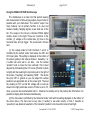
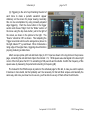
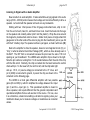
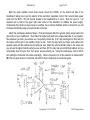
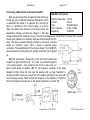
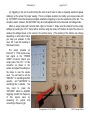
Laboratory 4
page 1 of 9
Laboratory 4
Exploring AC Waveforms
Parts List
Introduction
In this lab you will use the BLIP to generate periodic
waveforms (sine, triangle, and square) and explore various
properties of these signals. You will build an audio amplifier with
a speaker and listen to the period waveforms, as well as ambient
noise and the signal from a microphone. You will use the
microphone to generate oscillatory feedback. In the process, you
will learn to use an oscilloscope to look at signals and measure
their frequency and period.
Before you do anything else, make sure that the 9 V battery is
not connected to the breadboard. Power for this lab will come
only from the BLIP.
Last printed 11/1/14 6:34 PM
BLIP board (operational)
LM386 audio amplifier
speaker, 8 Ω, 0.5 watt
Electret Condenser Microphone
(WM-60PC)
100K potentiometer
26 gauge multi-stranded wire
velcro square with self-adhesive
various 5% resistors
various capacitors
© 2012 George Stetten
Laboratory 4
page 2 of 9
Using the RIGOL DS1102E Oscilloscope
The Oscilloscope is a basic tool that permits viewing
and measurement of time-varying signals, beyond what is
possible with your multi-meter. The modern “scope” has
many features, but its primary function is to view and
measure rapidly changing signals, as we shall see in this
lab. The scopes in the lab are 2-channel RIOGL digital
models, shown to the right. There are 3 sections to the
controls: (1) voltage on the vertical axis, (2) time on the
horizontal axis, and (3) trigger. We review each of these
next.
(1) The voltage scale for both Channels 1 and 2 is
controlled by the vertical “scale” knob above the CH1 and
CH2 input jacks. The setting is displayed at the bottom of
the screen (yellow) in the volts per division. Generally, 1 or
2 volt/div will work well in our labs. Use the vertical
“position” knob to move the trace vertically. This is best
adjusted by first selecting the CH1 menu (lit button in photo
to right) and then pushing the top button just to the right of
the screen (“Coupling”) and selecting “GND”. This shorts
the input CH1 to ground so you can adjust the vertical
position to an appropriate line on the screen grid. Then set
the coupling to “DC” so that DC voltage will be read (as
shown to the right) and make sure the “Probe” is set to 1X,
since your probe has no attenuation built in. Channel 2 is similarly set by first pushing the CH2 button. It is
possible to display both channels simultaneously.
(2) The time scale is controlled by the horizontal “scale” knob with the setting displayed on the bottom of
the screen (blue). The trace can be very slow (1 sec/div) to see entire events, or fast (1 msec/div to
1µsec/div) to see details of waveforms. The horizontal “position” knob moves the trace left and right.
Last printed 11/1/14 6:34 PM
© 2012 George Stetten
Laboratory 4
page 3 of 9
(3) Triggering is the act of synchronizing the start of
each trace to make a periodic waveform appear
stationary on the screen for proper viewing. Generally
this can be accomplished by using manually adjusted
edge triggering. Push the menu button in the trigger
section and choose “Edge” from the “Mode” section of
the menu using the top menu button, just to the right of
the screen, as shown in the picture to the right. The
“Source” should be CH1 as shown. Then adjusting the
Trigger Level knob will move the orange trace (shown to
the right, labeled “T”) up and down. When it intersects a
rising edge of the signal trace, triggering should function
properly producing a stable trace.
Attach a scope probe (with red and black clips) to CH 1 input as shown in the top photo on the previous
page, connecting the red and black clips to the internal ~3 V, 1 KHz square wave test signal in the lower right
corner of the front panel. Set CH 1 to something to 500 µsec/div and 2 volts/div. Confirm the frequency of this
square wave by measuring it’s period and converting to frequency (A)
The manual for the RIGOL scope is posted on the schedule page for this lab, in case you want to explore
it features in more detail, but that probably won’t be necessary for this lab. Most scopes work basically the
same way, and once you know how to use one, you’ll be able to use any of them without much trouble.
Last printed 11/1/14 6:34 PM
© 2012 George Stetten
Laboratory 4
page 4 of 9
Listening to Signals with an Audio Amplifier
Now construct an audio amplifier. It takes small time-varying signals in the audio
range (20 Hz - 20 KHz) and increases their voltage and current sufficiently to drive a
speaker. Let’s start with the speaker and work our way backwards.
Starting with two 1-foot pieces of fine 26 gauge multi-strand wire, strip ¼ inch
from the end of each, twist, tin, and bend into a hook. Insert the hooks into the lugs
on the speaker and carefully solder (don’t melt the plastic!). Wrap the wires around
the magnet to provide strain relief as shown. Solder short pieces of single strand 22
gauge wire to the other ends of the wires to plug into the breadboard, just as you did
with the 9 V battery clips. The speaker surface is just paper, so treat it with care. (B)
Next is the amplifier to drive the speaker, based on an integrated circuit (IC), or
“chip”, in what is called a Dual Inline Package (DIP), which we have already seen in
the BLIP. The DIP form is convenient because the pins have the same 1/10 inch
spacing as your breadboard. The LM386 audio amplifier chip is shown to the right.
Note the pin numbers, running from 1 to 8 counterclockwise from the end of the chip
with the little notch. Normally, the chip is inserted into the board across the central
divide with pin 1 in the lower left, the notch to left, and the chip label right
side up. Pin 6, VS (source voltage) is connected to the +5 V bus, and
pin 4 (GND) is connected to ground, to power the chip, as shown in the
LM386
schematic on the following page.
Top view
The LM386 is a fixed gain differential amplifier with two possible
gains (20 and 200) by which it amplifies the voltage between the +input
(pin 3) and the –input (pin 2). This specialized amplifier is meant to
drive a speaker, and is quite different than the general comparators and
operational amplifiers that we will use later in the course. For now, view
it as a black box, a basic tool enabling us to listen to signals, just as your
multimeter allows you to measure voltages or resistances as numerical
values.
Last printed 11/1/14 6:34 PM
© 2012 George Stetten
Laboratory 4
page 5 of 9
Build the audio amplifier circuit shown below around the LM386, on the bottom left side of the
breadboard, taking care to get the polarity of the electrolytic capacitors correct. Run red and black power
wires from the BLIP’s +5V and Ground outputs to the breadboard as in Lab 3. Note the use of a 1 µF
capacitor (all by itself in the upper right hand corner of the schematic) to stabilize the power supply.
Occasionally this circuit has been known to oscillate, due to internal feedback similar to that which you will
introduce intentionally using a microphone later in this lab.
Attach the oscilloscope leads as follows. First (and always!) attach the ground (black) scope lead to the
ground bus of your breadboard. Then attach the signal (red) lead to the ungrounded side of your speaker.
Now whatever you hear, you will also see. Temporarily include the 10 µF cap (boosts gain to 200) and turn
the volume control (pot in the amplifier circuit) to max. Touch the input with your finger, and examine the
speaker output with the oscilloscope and with your ears. Adjust the vertical volts/div scale on the scope until
you can see the signal. Describe what you see and hear. (C) You may hear a local AM radio station, and you
will probably hear 60 cycle “hum” from power sources around you. Using the oscilloscope, look for 60 Hz
hum setting the horizontal time scale accordingly. What is its period of a 60 Hz waveform in milliseconds?
(D) This is a good number to remember, since 60 Hz hum is frequently an unwelcome guest.
Last printed 11/1/14 6:34 PM
© 2012 George Stetten
Laboratory 4
page 6 of 9
Connecting a Microphone to the Audio Amplifier
WM-60PC microphone
Next, you will connect the microphone (“mike”) that your
Signal-to-noise ratio >40 dB
TA will give you, an Electret Condenser Microphone, which
Current
0.5 mA
is essentially two plates of a capacitor (the old word for
Type
Omnidirectional
which is “condenser”) with a fixed charge Q on them.
Freq. response
20 Hz–12 KHz
When the plates move because of incoming sound, the
Sensitivity
54 dB SPL
capacitance changes, and thus the voltage V = Q/C also
changes. Because the charge is very tiny, the mike is packaged with a Field Effect Transistor (FET) amplifier
whose input impedance is extremely high (we will learn about the FET
later). The mike is powered through a resistor to its output, a method
known as “phantom” power, since it avoids a separate power
connection. The specifications for the mike are shown. The 54 dB SPL
(sound pressure level) describes the quietest sound that can be picked
up.
Build the circuit below. Remove the 10 µF cap from the audio amp
to switch the gain from 200 to 20. The “mike” is powered through the
2.4 K output resistor. Have someone talk into the mike while you
report sound quality at speaker. (E) The low frequency response of the small
speaker is limited. Move the mike near the speaker until you hear “feedback”, a
runaway condition caused by sound from the speaker returning to the mike with
ever-increasing volume. What controls the frequency of the feedback? Explain in
terms of the speed of sound in air vs. the speed of electrons in a circuit. (F)
bottom view
Last printed 11/1/14 6:34 PM
© 2012 George Stetten
Laboratory 4
page 7 of 9
Looking at, and Listening to, the Sine, Triangle, and Square Waves
Remove the microphone and 2.4 KΩ resistor from the input of the audio amplifier. Run a white signal lead
from the BLIP’s I/O header pin 1 (Signal Generator Output) to a blank column on the breadboard and then
connect a 1 MΩ resistor from that to the input of the audio amplifier as shown in the circuit below.
In the previous lab, you used the BLIP in Data Acquisition
Mode. In the present lab, you will set the BLIP to Signal
Generator Mode by having a jumper at pin 40 and no jumper
at pin 39. You will then select sine, triangle, and square
waves using jumpers at pins 38 and 37, as defined in the table
to the left. Begin with jumpers in the sine wave setting.
Remember that the state of the jumpers is only read when you push the Reset button.
Signal Generator waveform jumpers
Signal Type
Pin 38
Pin 37
Square Wave
yes
yes
Sine Wave
no
yes
Triangle Wave
no
no
The periodic waveforms generated by the BLIP (sine, triangle, and square) can be varied in frequency
between approximately 460 Hz and 6.8 kHz by adjusting the potentiometer on the BLIP. Open a new
document in Microsoft Word on your computer and click the mouse in the document. Pressing the top button
on the BLIP (not the Reset button) will now type the present frequency (Hz) of the waveform on the computer
through the USB. Adjust the frequency of the sine wave, reporting 4 different frequencies from the computer
and their corresponding periods as shown on the scope. Show that frequency is the inverse of period. (G)
Adjust the BLIP to 600 Hz and listen. Now adjust to 900 Hz, 3/2 the original frequency. These two
frequencies should sound like the first and second notes in “Twinkle, twinkle, little star…”, an interval called
the perfect fifth. The ear likes small whole number ratios. Adjust to 1200 Hz, or twice the original frequency.
This is called an octave, and in a way sounds like the same note as the original 600 Hz, only higher. (H)
Returning to 600 Hz, listen to the sine wave carefully. Then, using the waveform table given earlier,
change the jumpers on pins 38 and 37 to give first the triangle wave and then the square wave. Describe the
differences in tone. (I)
Keep the audio amplifier assembled
on your breadboard. It is a handy tool
and you will use it in later labs.
Last printed 11/1/14 6:34 PM
© 2012 George Stetten
Laboratory 4
page 8 of 9
Using the Old Tektronics Oscilloscope
The Tektronix Oscilloscope in the lab (there should be
~12) is a basic tool that permits the viewing and measurement
of time-varying signals, beyond what is possible with your
multimeter. The oscilloscope, or simply “scope”, has many
features that are beyond this lab. In the first encounter, you
will simply use it view and measure rapidly changing signals.
The User Manual for the Tektronix 200 series scope can
be downloaded from the class schedule (next to this week’s
lab). You shouldn’t need it, however. Just be sure the settings
are correct for the 5 buttons to the right of the screen, as
described on the following page. Most of the scopes in the lab
are the 2-channel model (right, top), although one or two may
be 4-channel (right, bottom). They both share the same basic
adjustments of all scopes, (1) voltage on the vertical axis, (2)
time on the horizontal axis, and (3) triggering.
(1) The voltage scale is controlled by the “VOLTS/DIV”
(volts per division) knob above each input jack. The setting is
displayed on the screen. Generally, 1 volt/div will work well in
today’s lab. Use the “POSITION” knob for each channel to
move that trace vertically.
(2) The time scale is controlled by the SEC/DIV” (seconds
per division) knob, with the setting displayed on the screen.
The trace can be very slow (1 sec/div) to see entire events, or
fast (1 msec/div to 1µsec/div) to see details of waveforms.
The horizontal “POSITION” knob moves the trace left and
right.
Last printed 11/1/14 6:34 PM
© 2012 George Stetten
Laboratory 4
page 9 of 9
(3) Triggering is the act of synchronizing the start of each trace to make a repeating waveform appear
stationary on the screen for proper viewing. This is a complex operation, but luckily your scope comes with
an “AUTOSET” button that should accomplish satisfactory triggering to view the waveforms in this lab. You
should be aware, however, that AUTOSET may also make adjustments to the timescale and voltage scale.
Attach a scope probe (with red and black clips) to Channel 1. Make sure the channel has the proper
settings by pressing the “CH 1” menu button, and then using the column of 5 buttons to right of the screen to
achieve the settings shown on the screen in the picture below. (The meaning of the buttons can change
depending on what other button
you have just pressed. In this
case, CH 1 sets the meaning to
that shown below).
The scope provides an
internal 5 V, 1 KHz square wave
test signal at the “PROBE
COMP” connector. Attach your
scope probe from CH 1 to this
connector as shown in the
picture and adjust the settings on
the scope to view the square
wave. You will need to set the
“SEC/DIV” to something like 500
µsec/div. and “VOLTS/DIV” to
something like 2 volts/div. You
may
need
to
press
the
“AUTOSET” button to establish
triggering. Confirm the frequency
of this square wave by
measuring it’s period and
converting to frequency (J)
Last printed 11/1/14 6:34 PM
© 2012 George Stetten