Download GSS Sensor User`s Manual

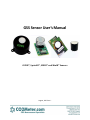
GSS Sensor User’s Manual
COZIR™, SprintIR™, MISIR™ and MinIR™ Sensors
August, 2015 Rev. I
Table of Contents
1
2
3
4
5
6
7
8
9
Guidelines for All Sensors ..................................................................................................................... 5
1.1
Power Supply ................................................................................................................................ 5
1.2
Calibration Procedure ................................................................................................................... 5
1.3
Ambient Sensors ........................................................................................................................... 5
1.4
Wide‐Range Sensors ..................................................................................................................... 5
1.5
Physical Configuration .................................................................................................................. 5
1.6
Dynamic Power Requirements ..................................................................................................... 6
Serial Format and Connection .............................................................................................................. 7
2.1
Connection .................................................................................................................................... 7
2.2
Serial Connection .......................................................................................................................... 8
2.3
Reading Format ............................................................................................................................. 8
2.3.1
CO2 Measurement ................................................................................................................. 8
2.3.2
Temperature Measurement (Optional) ................................................................................ 9
2.3.3
Humidity Measurement (Option) ....................................................................................... 10
2.3.4
Example of T,H and CO2 ...................................................................................................... 10
Command Summary ........................................................................................................................... 11
Operating Modes ................................................................................................................................ 13
4.1
Mode 0 Command Mode ........................................................................................................... 13
4.2
Mode 1 Streaming Mode ........................................................................................................... 13
4.3
Mode 2 Polling Mode ................................................................................................................. 13
Output Fields ....................................................................................................................................... 14
Zero Point Calibration ......................................................................................................................... 15
6.1
Zero in a Known Gas Concentration (recommended) ................................................................ 15
6.2
Zero in Nitrogen .......................................................................................................................... 15
6.3
Zero in Fresh Air (assumed to be 400ppm) ................................................................................. 15
6.4
Fine Tune the Zero Point ............................................................................................................. 16
6.5
Zero Point Adjustment ................................................................................................................ 16
AutoCalibration ................................................................................................................................... 16
7.1
Principle of Operation ................................................................................................................. 16
7.2
Requirements for Auto‐calibration ............................................................................................. 17
7.3
Setting the Auto Calibration Parameters .................................................................................... 17
7.4
Autocalibration Intervals............................................................................................................. 18
7.5
Read the Autocalibration Settings .............................................................................................. 19
7.6
Disable Autocalibration ............................................................................................................... 19
7.7
Background Concentration ......................................................................................................... 19
Altitude Compensation ....................................................................................................................... 20
User Settings ....................................................................................................................................... 22
9.1
Digital Filter ................................................................................................................................. 22
9.1.1
Customizing the Sensor Response ...................................................................................... 22
9.1.2
Setting the Digital Filter ...................................................................................................... 23
9.1.3
Reading the Digital Filter Setting ........................................................................................ 23
9.2
User Options – EEPROM Settings................................................................................................ 23
9.2.1
Setting EEPROM .................................................................................................................. 24
2
9.2.2
Reading EEPROM ................................................................................................................ 24
9.2.3
EEPROM Settings................................................................................................................. 24
9.2.4
Autocalibration Settings (locations 3‐7).............................................................................. 25
9.2.5
User EEPROM ...................................................................................................................... 25
10 Command Reference .......................................................................................................................... 26
10.1 Customization ............................................................................................................................. 26
10.2 Information ................................................................................................................................. 27
10.3 Switching between Modes .......................................................................................................... 28
10.4 Zeroing and Calibration ............................................................................................................... 28
10.5 Polling Commands ...................................................................................................................... 30
11 Appendix A: Power Consumption ....................................................................................................... 32
11.1 Operating Modes – Power Levels ............................................................................................... 33
11.2 Streaming Mode (K 1) ................................................................................................................. 33
11.3 Polling Mode (K 2) ....................................................................................................................... 33
11.4 Command Mode (K 0) ................................................................................................................. 33
11.5 Current Profile............................................................................................................................. 34
11.6 Warm‐up Time ............................................................................................................................ 35
11.7 Minimizing the Power in Streaming and Polling Modes ............................................................. 37
11.8 Polling and Streaming Key Points ............................................................................................... 37
11.9 Minimizing Power using Command Mode .................................................................................. 38
11.10
Command Mode Power Reduction Key Points ....................................................................... 39
11.11
Minimizing Power by Power Cycling ....................................................................................... 40
11.12
Power Cycling Key Points ........................................................................................................ 41
11.13
Implementing a User Auto‐Calibration Routine ..................................................................... 42
12 Appendix B: Analog Voltage Output ................................................................................................... 43
12.1 Ordering Information .................................................................................................................. 43
12.2 Voltage Output Connections ....................................................................................................... 44
12.3 Load Impedance .......................................................................................................................... 44
12.4 Converting Voltage to Concentration ......................................................................................... 44
12.5 Linearity of the Voltage Output .................................................................................................. 45
12.6 Noise on the Voltage Output ...................................................................................................... 46
12.7 Changing the Full Scale Concentration ....................................................................................... 46
12.8 Digital outputs ............................................................................................................................. 47
12.9 Zero Point Calibration ................................................................................................................. 47
13 Appendix C: Setting the Auto‐Calibration Parameters for Older Firmware ....................................... 48
13.1 Environmental Requirements for Auto‐calibration .................................................................... 48
13.2 Auto‐calibration using GasLab® ................................................................................................... 48
13.3 Setting the Auto Calibration Parameters .................................................................................... 48
13.4 Background Concentration ......................................................................................................... 49
13.5 Auto‐calibration Interval ............................................................................................................. 49
13.6 Initial Auto‐calibration period ..................................................................................................... 50
13.7 Auto‐Calibration Examples.......................................................................................................... 51
3
This documentation is provided on an as‐is basis and no warranty as to its suitability or accuracy for any
particular purpose is either made or implied. Neither CO2Meter, Inc. nor Gas Sensing Solutions Ltd will
accept any claim for damages howsoever arising as a result of use or failure of this information. Your
statutory rights are not affected. This information is not intended for use in any medical appliance,
device or system in which the failure of the product might reasonably be expected to result in personal
injury. This document provides preliminary information that may be subject to change without notice.
This guide applies to software versions from July 2013. For previous versions, please refer to ‘COZIR
Software USER’s Guide Rev F’
Conventions
In this guide:
\r\n
Is used to indicate carriage return <CR> , line feed <LF> characters, (0x0d,0x0a) which are required at
the end of each string sent to the sensor, and are appended to all transmissions from the sensor.
‐A denotes an ambient model sensor. –W denotes a wide‐range sensor.
Z 12345\r\n
Courier fixed pitch font is used to show commands sent to the sensor, and transmissions received from
the sensor.
RoHS Certification
GSS Ltd. hereby certifies that the COZIR, SprintIR and MISIR products are RoHS compliant and fulfils the
definitions and restrictions defined under Directive 2011/65/EU of The European Parliament and of the
Council of June 8, 2011 on the restriction of the use of certain hazardous substances in electrical and
electronic equipment (EEE).
RFI & CE Certification
The COZIR family of sensors has been used in client and GSS products which have successfully passed
through full CE certification. This includes radiated noise immunity as per EN61000‐4‐3: 2006 Type 1
80 – 1000MHz, 3V/m, 80%, 1kHz AM
1400 – 2000, 3V/m, 80%, 1kHz AM
2000 – 2700MHz, 1V/m, 80%, 1kHz AM
To minimise issues with noise immunity we recommend the following:
 Add a decoupling capacitor across the supply close to the sensor.
 If you are using a switched mode supply, use shielded inductors, and locate away from the
sensor. This also applies to other magnetic components such as electromagnetic buzzers.
 Always adhere to the respective manufacturer’s advice on PCB layout for switched mode power
supply devices.
 Avoid routing power tracks or leads across the sensor.
4
1 Guidelines for All Sensors
To achieve maximum precision when integrating the GSS line of sensors into a product, we recommend
following these guidelines. We have developed these requirements after rigorous testing to maximize
the performance and accuracy of the sensor in the host application.
1.1 Power Supply
The sensors must be powered with a linear regulator for maximum precision. Power supplies with high
frequency noise, such as switching supply circuits, can cause increased noise in the sensor’s measured
value.
Altering the power supply will require recalibration. We recommend calibrating the sensor in its final
installation, calibrating the sensor outside with a different configuration will yield inconsistent
calibration results.
1.2 Calibration Procedure
We recommend calibrating all sensors. The procedure differs between models. Calibration gas is
available from CO2Meter directly.
1.3 Ambient Sensors
For ambient sensors we recommend an atmospheric calibration. Fresh air is generally assumed to be at
450ppm, but alternatively you can use 450ppm calibration gas.
This reading can be confirmed with 2,000ppm calibration gas to check the span of the sensor, although
this step is unnecessary.
1.4 Wide‐Range Sensors
For wide‐range sensors, we recommend a zero calibration using an end‐of‐range 95% gas.
This reading can be confirmed with other high‐concentration CO2 calibration gases, such as 50% and
25%, although this step is unnecessary.
1.5 Physical Configuration
The sensor can be configured with optional tube caps, available through our website, or simply in an
atmospheric sampling configuration. The configuration must be kept consistent between calibration and
installation. Calibrating with a different setup will result in inaccurate readings when installed.
When using a sensor without a tube cap, we recommend ensuring turbulence is present across the
sensor membrane. This can be achieved with a calibration chamber featuring a recirculation fan or
constant flow from a fixed‐flow regulator.
5
1.6 Dynamic Power Requirements
Bench‐tested results for ultra‐low power sensors powered via USB
Dynamic power requirements become important when operating from a USB port where the supply
current might be being shared over several ports (we recommend using powered USB hubs to avoid
these potential power issues) or when planning for low power applications like solar power.
When the power is applied to the sensor, initially a higher than normal operating current demand will
occur. This inrush current and period will relate to the impedance of the power supply and device
switching power.
The measurements below were taken whilst connected to a USB port via a USB to UART bridge cable,
3.3 volts, streaming / poled mode, and same interval of measurement on a COZIR sensor.






Quiescent: 300 uA
Measurement interval: 500 mS
Measurement period: 20ms
Measurement current: 30 mA
RMS operating power: 2 uW
Startup inrush current 50 mS @ 60 mA peaks
6
2 Serial Format and Connection
2.1 Connection
Communication to and from the various sensors is via a serial connection. Pins are shown looking at the
connector of the sensor.
COZIR‐Ambient
GND
3.3V
Rx
Tx
N/C
N/C
N/C
N/C
Zero
Ambient
COZIR‐Wide Range, SprintIR
MISIR
MinIR
GND
V+
0v
3.3‐5.5V (3.3V recommended)
Tx‐OUT
Rx‐IN
Voh will be 3V Sensor output
Used for configuration, etc.
7
2.2 Serial Connection
The Rx and Tx pins are normally high, suitable for direct connection to a UART. If the sensor is to be read
by a true RS232 device (eg a PC) it is necessary to pass through a level converter to step up/down the
voltage and invert the signal.
Connection to the sensor is via a 10 way, 0.1” pitch connector. In practice, only the first 4 pins are
required (GND, 3V3, Rx and Tx) so a 4 way connector can be used.
A Development kit and free GasLab® software is available to allow USB interfacing between COZIRTM and
SprintIRTM sensors and a PC. Contact CO2Meter.com for details.
Parameter
Baud Rate
Value
9600
Data Bits
Parity
Stop Bits
8
None
1
Format
Hardware Flow Control
Voltage Voh
UART (normally high)
None
3V (MISIR Voh = Vsupply)
Voltage Vih
3V‐5V
Note: If you connect to the sensor using HyperTerminal®, you must select the box “Send line ends with
line feeds” under ASCII setup.
When initially powered, the sensor will immediately start to transmit readings (see Mode 1 in
“Operating Modes”)
2.3 Reading Format
2.3.1 CO2 Measurement
The CO2 measurement is reported as:
Z ##### z #####\r\n
where
Z ##### shows the CO2 concentration after digitally filtering
and
z ##### shows the instantaneous CO2 concentration without any digital filtering.
8
The concentration is reported in the following units
Type
Range
Units
Example
COZIR‐A
MISIR
COZIR‐W
SprintIR‐W
MinIR‐5
COZIR‐W‐100
SprintIR‐W‐100
MinIR‐100
Up to 2%
ppm
Z 00631 = 631ppm
Up to 65%
ppm/10
Z 01200 = 12000ppm = 1.2%
Up to 100%
ppm/100
Z 01500 = 150000ppm = 15%
Note that the same units must be used when sending concentration information to the sensor (for
example, the X command and the F command). If in doubt, the ‘.’ Command (see below) will indicate
what multiplier should be applied to the Z output to convert to ppm.
Z
Z
Z
Z
Z
Z
Z
Z
Z
Z
Z
00842
00842
00842
00842
00842
00842
00842
00842
00842
00842
00842
z
z
z
z
z
z
z
z
z
z
z
00765
00738
00875
00858
00817
00839
00817
00828
00850
00875
00804
Sample output from a sensor with factory
settings.
This is a COZIR‐A, so the reported CO2 reading
is 842ppm.
The second figure shows the instantaneous
(unfiltered) CO2 reading.
See “Digital Filter” for more details.
Note that all output from the sensor has a leading space.
2.3.2
Temperature Measurement (Optional)
The temperature measurement is reported as:
T #####\r\n
where ##### is a five digit number.
To convert to ºC, subtract 1000 and divide by 10.
For example:
T 01235\r\n
Represents 23.5ºC
NB The temperature and humidity sensor is a factory fit option. If it is not fitted, the sensor will return “T
01000”.
9
2.3.3 Humidity Measurement (Option)
The humidity measurement is reported as:
H #####\r\n
Where ##### is a five digit number.
To convert to relative humidity (%), divide by 10.
For example:
H 00551\r\n
Represents 55.1% RH
NB The temperature and humidity sensor is a factory fit option. If it is not fitted, the sensor will return
“H 00000”.
2.3.4
Example of T,H and CO2
When shipped, the sensor default output is CO2 only. To output temperature, humidity and CO2, send
“M 4164\r\n” (see “Output Fields”). The output format will have the form:
H 00345 T 01195 Z 00651\r\n
This example indicates 34.5% RH, 19.5ºC and 651ppm CO2
10
3 Command Summary
For complete details of the commands and their correct usage, please refer to the “Command
Reference”.
IMPORTANT:

All commands must be terminated with a carriage return and line feed <CR><LF>. In this document, this
is shown as ‘\r\n’.

Commands which take a parameter always have a space between the letter and the parameter.

The sensor will respond with a ‘?’ if a command is not recognized. The two most common causes are
missing spaces or missing <CR><LF> terminators.
Command
Use
Example
Response
Comments
A ###\r\n
a\r\n
Set the digital Filter
Return the digital
filter setting
Fine Tune the zero
point
Zero point
calibration using
fresh air.
Return most recent
humidity
measurement
Selects the
operating mode
Sets the output
fields
Sets a user
configurable field in
EEPROM
Reads a user‐
configurable field
from EEPROM
Return most recent
fields
Sets the span
calibration value
Return the span
calibration value
Return the most
recent temperature
measurement
Zero point
calibration using
nitrogen.
Manual setting of
the zero point.
Zero point setting
using a known gas
calibration
A 16\r\n
a\r\n
A 00016\r\n
a 00016\r\n
See “User Settings”
See “User Settings”
F 410 400\r\n
F 33000\r\n
See “Zero Point Calibration”
G\r\n
G 33000\r\n
See “Zero Point Calibration”
H\r\n
H 00552\r\n
K 1\r\n
K 00001\r\n
=55.2% in the example.
Humidity sensing is a factory
fit option.
See “Operating Modes”
M 6\r\n
M 00006\r\n
See “Output Fields”
P 1 10\r\n
P 00001 00010\r\n
See “User Settings”
p 10\r\n
p 00010 00001\r\n
See “User Settings”
F ##### #####\r\n
G\r\n
H\r\n
K #\r\n
M #####\r\n
P ### ###\r\n
p ###\r\n
Q\r\n
S #####\r\n
s\r\n
T\r\n
U\r\n
u #####\r\n
X #####\r\n
Q\r\n
See “Command Reference”
S 8192\r\n
S 08192\r\n
See “Span Calibration”
s\r\n
s 08192\r\n
See “Span Calibration”
T\r\n
T 01225\r\n
U\r\n
U 33000\r\n
22.5⁰C in the example.
Temperature sensing is a
factory fit option.
See “Zero Point Calibration”
u 32997\r\n
u 32997\r\n
See “Zero Point Calibration”
X 2000\r\n
X 32997\r\n
See “Zero Point Calibration”
11
Command
Use
Example
Response
Comments
Y\r\n
Return firmware
version and sensor
serial number
Return the most
recent CO2
measurement.
Autocalibration
configuration
Return the
multiplier required
to convert the Z
output to ppm
Return
configuration
information.
Y\r\n
Returns two lines
See “Command Reference”
for details
Z\r\n
Z 01521\r\n
1521ppm in the example
@ 1.0 8.0\r\n
@ 1.0 8.0\r\n
.\r\n
. 00100\r\n
See “Autocalibration” for
details
Multiply by 100 in the
example
Z\r\n
@ #.# #.#\r\n
.\r\n
*\r\n
*\r\n
See the “Command
Reference” for details
All communications are in ASCII and are terminated by carriage return, line feed (ASCII characters 13 and
10). This document uses the protocol “\r\n” to indicate the carriage return line feed.
All responses from the sensor, including measurements, have a leading space (ASCII character 32).
The character ‘#’ represents an ASCII representation of a numeric character (0‐9).
Note that there is a space between the first letter and any parameter. For example, the X command
reads “X space 2000 carriage return line feed”.
Note that all settings are stored in non‐volatile memory, so the sensor only has to be configured once.
It should not be configured every time it is powered up.
12
4 Operating Modes
The COZIR™, SprintIR™, MISIR™ and MinIR™ sensors can be operated in three different modes. Users
can switch between the modes using the “K” command.
4.1 Mode 0
Command Mode
This is primarily intended for use when extracting larger chunks of information from the sensor (for
example using the Y and * commands).
In this mode, the sensor is stopped waiting for commands. No measurements are made, and the sensor
will run through a warm‐up cycle after exiting this command. There is no latency in command responses.
The power consumption is less than 3.5mW as no measurement activity takes place. Commands which
report measurements or alter the zero point setting are disabled in mode 0.
Mode 0 is NOT retained after power cycling. The sensor will always power up in streaming or polling
mode, whichever was the most recently used.
4.2 Mode 1
Streaming Mode
This is the factory default. Measurements are reported twice per second for COZIR, MinIR and MSIR
sensors and 20 times per second for SprintIR sensors. Commands are processed when received, except
during measurement activity, so there may be a time delay of up to 100mS in responding to commands.
The power consumption is 3.5mW (assuming one field of information is transmitted, and there is no
temperature and humidity sensor).
4.3 Mode 2
Polling Mode
In polling mode, the sensor only reports readings when requested. The measurement cycle continues in
the background, but the output stream is suppressed. The power consumption depends on the
frequency of polling, but is approximately the same as the streaming mode power consumption.
Note that the sensor will power up in the mode last used. If it was last used in K0 mode, it will power up
in either K1 or K2 mode, depending on which was most recently used.
In Polling Mode, measurements can be accessed using the polling commands H, L, Q, T and Z (see
“Command Reference”).
13
5 Output Fields
The COZIR™ sensor can be configured to output up to five fields of information. Typically, the only fields
of interest are the CO2 concentration, Temperature (if fitted) and Humidity (if fitted).
This allows users to customize the output string transmitted by the sensor. Up to five values can be
transmitted in the string. The format is always the same: each field is identified by a single character,
followed by a space, followed by the five digit number indicating the value of the parameter.
The output fields can be set by sending a command of the format M 12345\r\n where 12345
represents a mask value which defines the output fields.
The mask value is created by adding the mask values for the parameters required (see table below).
The sensor will output a maximum of five fields. If the mask setting represents more than five fields,
only the first five (those with the highest mask values) will be output.
SprintIR sensors have a limited time to transmit information, so no more than two fields should be
selected for output.
Parameter
Field
Identifier
Mask
Value
Comments
Reserved
Reserved
Reserved
Humidity
H
32768
16384
8192
4096
D digitally filtered
d
2048
D unfiltered
Reserved
Zero Set Point
Sensor Temperature
(unfiltered)
Temperature
D
h
V
1024
512
256
128
T
64
LED Signal (digitally
filtered)
LED Signal (unfiltered)
o
32
O
16
Sensor Temperature
(filtered)
CO2 Output (Digitally
Filtered)
CO2 Output (not
filtered)
Reserved
v
8
Z
4
Reserved
Reserved
Reserved
Reports the humidity output of the Temperature and Humidity
Sensor (if Fitted).
Reports a value related to the normalized LED signal strength
(smoothed)
Reports a value related to the normalized LED signal strength
Reserved
Reports a value related to the normalized LED signal strength
Reports a value which varies inversely with the sensor
temperature.
Reports the temperature output of the Temperature and
Humidity Sensor (if Fitted).
Reports a value which gives an indication of the LED signal
strength (smoothed)
Reports a value which gives an indication of the LED signal
strength.
Reports a value which varies inversely with the sensor
temperature. (smoothed)
Digitally filtered CO2 reading
z
2
Instantaneous CO2 reading
1
Reserved
Note that most fields are for advanced use only and require specific guidance from GSS engineering for
their correct interpretation and use. Measurement field are indicated in bold.
14
For example, to output the temperature, humidity and CO2 measurements, send:
M 4164\r\n
The output string will then be:
H 12345 T 12345 Z 00010\r\n
6 Zero Point Calibration
There are a several methods to calibrate the zero point of the sensor. The recommended method is zero
point calibration in a known gas (see X command) which will give the most accurate zero setting.
In all cases, the best zero is obtained when the gas concentration is stable and the sensor is at a
stabilized temperature.
6.1 Zero in a Known Gas Concentration (recommended)
Place the sensor in a known gas concentration and allow time for the sensor temperature to stabilize,
and for the gas to be fully diffused into the sensor.
Send the command X ###\r\n
The concentration must be in the same units as the sensor output (see “Reading Format”. The sensor
will respond with an echo of the command and the new zero point.
For example, to set the zero point in a COZIR‐A when the sensor is in a known gas concentration of
2000ppm
send:
response:
X 2000\r\n
X 32950\r\n
6.2 Zero in Nitrogen
Place the sensor in a gas containing no CO2 (typically nitrogen) and allow time for the sensor
temperature to stabilize, and for the gas to be fully diffused into the sensor.
Send the command U\r\n
The sensor will respond with an echo of the command and the new zero point.
For example,
send:
response:
U\r\n
U 32950\r\n
6.3 Zero in Fresh Air (assumed to be 400ppm)
If there is no calibration gas and no nitrogen available, the sensor zero point can be set in fresh air. The
sensor is programmed to assume that fresh air is 400ppm (this value is user configurable – see “User
Settings”).
15
Place the sensor in a fresh air environment and allow time for the sensor temperature to stabilize, and
for the fresh air to be fully diffused into the sensor.
Send the command G\r\n
The sensor will respond with an echo of the command and the new zero point.
For example,
send:
response:
G\r\n
G 32950\r\n
6.4 Fine Tune the Zero Point
If the CO2 concentration and the sensor reported concentration are known, the zero point can be
adjusted using the known concentration to fine tune the zero point. This is similar in operation to the
“X” command (see above) but can operate on historic data. For example, if the sensor has been in an
environment in which it is known to have been exposed to outside air, and the sensor reading is known
at that time, the zero point can be fine‐tuned to correct the reading. This is typically used to implement
automated calibration routines.
The command takes two parameters, separated by a space. The first parameter is the reading reported
by the sensor. The second is the corrected reading. Both parameters must be in the same units as the
sensor output (see “Reading Format”)
The sensor will respond with an echo of the command and the new zero point.
For example,
send:
response:
F 400 380\r\n
F 32950\r\n
In this example, the sensor zero point would be corrected so that a reading of 400ppm, would now be
reported as 380ppm.
6.5 Zero Point Adjustment
The precise zero point can be fine‐tuned by sending a zero point to the sensor. This is not recommended
for general use.
Send the command u #####\r\n where ##### is the new zero point.
7 AutoCalibration
7.1 Principle of Operation
COZIR sensors are fully calibrated prior to shipping from the factory. Over time, the zero point of the
sensor needs to be calibrated to maintain the long term stability of the sensor.
In many applications, this can happen automatically using the built in auto‐calibration function.
16
CO2 Concentration (ppm)
This technique can be used in situations in which sensors will be exposed to typical background levels
(400‐450ppm) at least once during the auto‐calibration period. For example, many buildings will drop
quickly to background CO2 levels when unoccupied overnight or at weekends. The auto‐calibration
function uses the information gathered at these periods to recalibrate.
One Week ‐>
This recording from a sensor shows a typical one week recording in an office environment. The auto‐
calibration function uses the low point (circled) and uses it to recalibrate the zero point.
7.2
Requirements for Auto‐calibration
Exposure to Fresh Air
The sensor must ’see’ fresh air at least once during the auto‐calibration period. You do not need to know
when the fresh air will be sensed, just that it will be sensed at some point during the period.
Continuously Powered
The auto‐calibration information is deleted when the sensor is switched off. This ensures that each
installation is unaffected by any previous history of the sensor. For auto‐calibration to function, it must
be power on for the whole of the auto‐calibration period.
7.3 Setting the Auto Calibration Parameters
Three parameters are required to enable the auto‐calibration routine:
Auto‐Calibration Interval
This determines how often the auto‐calibration takes place.
Background Concentration
17
Typically 400‐450ppm. This is the level the sensor will use as background.
Initial Auto‐calibration Interval
It is possible for the first auto‐calibration to take place more quickly than the regular auto‐calibration
event. This can be useful to stabilize quickly after installation.
Note that the autocalibration timers are reset when the power to the sensor is interrupted. On power
on, the sensor will always time an initial autocalibration interval first, then settle into the regular
autocalibration cycle.
The regular autocalibration timer is reset automatically if the user calibrates the sensor using the
U,G,X,F or u commands.
Before setting the auto‐calibration parameters, please note the following:
 Before altering the auto‐calibration parameters, switch the sensor into command mode:
send
K 0 <CR><LF>
This stops the measurement process in the sensor.

All commands must be terminated with \r\n (carriage return, line feed). NB HyperTerminal does
not add the line feed character as standard. The ASCII Setup must be configured to append line
feeds.
7.4 Autocalibration Intervals
The autocalibration intervals are set using the ‘@’ command. This command allows the autocalibration
periods to be set, interrogated or disabled.
To set the autocalibration intervals, the command structure is
@ initialinterval regularinterval\r\n
Where both the initial interval and regular interval are given in days. Both must be entered with a
decimal point and one figure after the decimal point.
For example
send:
response:
@ 1.0 8.0\r\n
@ 1.0 8.0\r\n
Will set the autocalibration interval to 8 days, and the initial interval to 1 day.
Note that there is a space between the @ and the first number, and a space between the two numbers.
In hex, the example above reads
40 20 31 2E 30 20 38 2E 30 0D 0A
18
7.5 Read the Autocalibration Settings
To determine the current autocalibration settings:
send:
response:
@ \r\n
@ 1.0 8.0\r\n
If the autocalibration is enabled, the sensor will respond with the format above showing the initial and
regular autocalibration intervals. If the autocalibration is disabled, the sensor will respond with
send:
response:
@ \r\n
@ 0\r\n
7.6 Disable Autocalibration
To disable the autocalibration:
send:
response:
@ 0\r\n
@ 0\r\n
ie, @ followed by a space followed by a zero terminated with 0x0d 0x0a
7.7 Background Concentration
The background concentration depends somewhat on the area the sensor is installed. Typically, a figure
between 400ppm and 450ppm is used. The factory default is 400ppm.
To set this, send
P 8 x\r\n
P 9 y\r\n
where x and y depend on the concentration you want to set.
Concentration
380
400
425
450
x
1
1
1
1
Y
124
144
169
194
This is stored as a two byte value, the high byte being in location 8 and the low byte in location 9.
The value represents the concentration.
19
To calculate other values,
x= int(concentration/256)
y= the remainder after dividing concentration/256
8 Altitude Compensation
Important
This feature was introduced in sensors manufactured after July 2013 using firmware version AL17 or
higher. The firmware version can be identified by sending the Y or * command.
Altitude compensation applies a permanent correction to the sensor response, so should only be used
when it is known that the sensor will be operating at altitude permanently.
NDIR gas sensors, such as the COZIR, SprintIR and MISIR family of sensors, detect the concentration of
gas by measuring the degree of light absorption by the gas analysis. The degree of light absorption is
then converted into a concentration reported by the sensor.
The absorption process is pressure dependent, so that a change in pressure will cause a change in the
reported gas concentration. As the pressure increases, the reported gas concentration also increases.
As the pressure decreases, the reported concentration decreases.
This effect takes place at a molecular level as is common to all NDIR gas sensors.
In normal use, the reading will vary by 0.1% of reading for each mbar change in barometric pressure (the
sensor are calibrated at 1013mbar).
If the sensor is installed at an elevated altitude, the mean barometric pressure will be lower than
1013mbar. It is possible to configure the sensor to correct for this effect, by setting the altitude when
installing. This will apply a permanent correction to the output of the sensor, depending on the altitude
setting selected.
To apply this correction,
1) Select the appropriate code from the table below (intermediate values can be interpolated)
2) Send the “S ####\r\n” to the sensor, where #### is the code from the table below.
For example, to correct the sensor for permanent installation at 305m elevation,
send:
response:
S 8494\r\n
S 08494\r\n
20
Altitude (ft.)
‐1000
0
1000
2000
3000
4000
5000
Altitude (m)
‐305
0
305
610
915
1219
1524
Barometric Pressure (mbar)
1050
1013
976
942
908
875
843
Code
7889
8192
8495
8774
9052
9322
9585
The current setting can be determined by sending a lower case s:
send:
response:
s\r\n
s 08494\r\n
21
9 User Settings
9.1 Digital Filter
9.1.1 Customizing the Sensor Response
The CO2 measurement is passed through a digital filter to condition the signal. The characteristics of
the filter can be altered by the user to tune the sensor performance to specific applications.
The filter operates as a low pass filter ‐ increasing the filter parameter reduces measurement noise, but
slows the response. There is a tradeoff between noise (resolution) and speed of response.
The filter can be set to a value between 1 and 65535. Settings larger than 64 are not recommended for
normal use. A low value will result in the fastest response to changes in gas concentration, a high value
will result in a slower response. Note that the response is also determined by the diffusion rate into the
sensor. The default setting is 32.
This chart shows the effect of changing the filter setting:
Sensor Noise
Sensor Noise vs Filter Setting
Filter Setting
Increasing the filter setting has a beneficial impact on noise, so improves the sensor resolution. It also
slows the sensor response to transients. This can be used to improve the detection of average CO2
conditions. In building control, for example, a fast response to breathing near the sensor is undesirable.
If the transient response is important either for speed of response or because the shape of the transient
is required, a low filter setting should be used.
The following chart shows the same transient event capture using a filter setting of 4, and using a filter
setting of 32.
22
Reported CO2
Effect of Filter on Transient Response
Filter = 4
Filter = 32
9.1.2 Setting the Digital Filter
To change the setting, type A ###\r\n where ### is the required filter setting.
For most applications, a filter setting of 32 is recommended.
send:
response:
A 32\r\n
A 00032\r\n
If the filter is set to zero, a smart filter mode will be used in which the filter response is altered to suit
the prevailing conditions. This is useful if there is a combination of steady state conditions, with some
periods of rapidly changing concentrations.
9.1.3 Reading the Digital Filter Setting
The current setting for the digital filter can be determined by sending a\r\n
send:
response:
a\r\n
a 00032\r\n
9.2 User Options – EEPROM Settings
Some user settings can be altered in the internal EEPROM.
These settings can be set by using the parameter setting command “P”, and read using a lower case “p”.
There are also 32 bytes of user EEPROM storage available.
23
9.2.1 Setting EEPROM
To set an EEPROM location, send
P ### ###\r\n
Where the first parameter is the address, and the second is the value.
Note that two byte values must be set one byte at a time.
For example, to change the default value of the ambient gas concentration used for ambient calibration
(i.e. the assumed CO2 concentration in fresh air) to 380ppm, send
send:
response:
send:
response:
P
P
P
P
10 1\r\n
00010 00001\r\n
11 124\r\n
00011 00124\r\n
9.2.2 Reading EEPROM
To read a parameter value from an EEPROM location, send “p #####\r\n” where ##### is the
address of the parameter.
Note that two byte values must be read one byte at a time.
For example, to read the value of the ambient gas concentration used for ambient calibration (ie the
assumed CO2 concentration in fresh air)
send:
response:
send:
response:
p
p
p
p
10\r\n
00010 00001\r\n
11\r\n
00011 00124\r\n
9.2.3 EEPROM Settings
Most of the EEPROM settings are two byte values, indicated by HI and LO in the variable name in the
following table. We recommend contacting GSS before altering the default values.
Location
0
1
2
Name
AHHI
ANLO_
ANSOURCE
Purpose
Reserved
Reserved
Reserved
Default Value
0
0
0
24
3
ACINITHI
4
5
ACINITLO
ACHI
6
7
8
ACLO
ACONOFF
ACPPMHI
9
10
ACPPMLO
AMBHI
11
12
AMBLO
BCHI
13
200‐231
BCLO
Autocalibration Preload. This preloads the
autocalibration timer so that the first autocalibration
occurs after a shorter time.
Low byte of above.
Autocalibration Interval. Sets the time interval
between autocalibrations.
Low byte of above.
Switches Autocalibration ON/OFF
Autocalibration Background Concentration. This
determines what background CO2 level is assumed
for autocalibration.
Low byte of above.
Ambient Concentration (for G command). This
determines what background CO2 level is assumed
for ambient calibration using the “G” command.
Low byte of above.
Buffer clear time. This will clear any incomplete
commands from the serial buffer after a fixed period
of inactivity. The time is in half second increments.
Low byte of above.
User EEPROM
87
192
94
128
0
1
194
1
194
0
8
255
9.2.4 Autocalibration Settings (locations 3‐7)
These are included now to maintain compatibility with previous firmware versions. We recommend
using the @ command to set autocalibration timings.
9.2.5 User EEPROM
Locations 200 to 231 can be used to store user values. Each location is a single byte. These locations are
not used by the sensor.
E.g. to store the number 42 in the first user EEPROM location:
send:
response:
P 200 42\r\n
P 00200 00042\r\n
and to read it
send:
response:
p 200\r\n
p 00200 00042\r\n
Note that the EEPROM is only guaranteed for 100,000 write cycles.
25
10 Command Reference
This gives the complete command set for the COZIR™, SprintIR and MISIR sensors and illustrates
use of some of the more commonly used options.
Key points to note are:
 In all cases, commands are terminated with a carriage return, line feed (“\r\n”).
 Commands are case sensitive.
 The commands use all use ASCII characters. Each command lists the ASCII letter and
includes the hex code for avoidance of doubt.
 Always check for a correct response before sending another command.
 If a command is unrecognized, the sensor will respond with a “?”
WARNING
This document is provided to give a complete reference of the command set and outputs from the
COZIR™ sensor. It is intended for advanced users only. If in doubt, please contact CO2Meter.com
prior to use.
10.1 Customization
A COMMAND (0x41)
Example:
USER CONFIGURATION
A 128\r\n
Description:
Set the value for the digital filter.
Syntax:
ASCII character 'A', SPACE, decimal, terminated by 0x0d 0x0a (CR & LF) Response:
A 00032\r\n
a COMMAND (0x61)
INFORMATION
Example:
a\r\n
Description:
Syntax:
Response:
Return the value for the digital filter.
ASCII Character 'a' terminated by 0x0d 0x0a (CR & LF)
a 00032\r\n
M COMMAND (0x4D)
USER CONFIGURATION
Example:
M 212\r\n
Description:
Syntax:
Determines which values are going to be returned by the unit.
"M", SPACE, followed by an up-to 5 digit number, each bit of which dictates which
item will be returned by the sensor, terminated by 0x0d 0x0a (CR & LF).
M 212\r\n
(see “Output Fields” for details)
Response:
26
P COMMAND (0x50)
USER CONFIGURATION
Example:
P 10 1\r\n
Description:
Syntax:
Sets a user configurable parameter.
"P", SPACE, followed by an up to 2 digit number, SPACE followed by an up to 3 digit
number, terminated by 0x0d 0x0a (CR & LF).
P 00001 00010\r\n
(see “User Settings” for details)
Response:
p COMMAND (0x70)
USER CONFIGURATION
Example:
p 10\r\n
Description:
Syntax:
Returns a user configurable parameter.
"P", SPACE, followed by an up-to 2 digit number, terminated by 0x0d 0x0a (CR &
LF).
P 10 1\r\n
(see “User Settings” for details)
Response:
10.2 Information
Y COMMAND (0x59)
INFORMATION
Example:
Y\r\n
Description:
Syntax:
Response:
the present version string for the firmware
ASCII character 'Y', terminated by 0x0d 0x0a (CR & LF)
Y,Jan 30 2013,10:45:03,AL17\r\n
B 00233 00000\r\n
NB This command returns two lines split by a carriage return line feed, and terminated by a carriage
return line feed. This command requires that the sensor has been stopped (see ‘K’ command).
* COMMAND (0x59)
Example:
INFORMATION
*\r\n
Description:
Returns a number of fields of information giving information about the sensor
configuration and behavior.
Syntax:
ASCII character '*', terminated by 0x0d 0x0a (CR & LF)
Response:
Contact GSS for details.
. COMMAND (0x2E)
Example:
INFORMATION
.\r\n
Description:
Returns a number indicating what multiplier must be applied to the Z or z output
to convert it into ppm.
27
Syntax:
Response:
ASCII character '.', terminated by 0x0d 0x0a (CR & LF)
00001\r\n”
(this number is variable).
10.3 Switching between Modes
For discussion of different modes of operation, see the section “Operating Modes”.
K COMMAND (0x4B)
Example:
Description:
Syntax:
Response:
USER CONFIGURATION
K 1
Switches the sensor between the operating modes.
ASCII character "K", SPACE, followed by the mode number, terminated by 0x0d
0x0a (CR & LF).
K 1\r\n
(the number mirrors the input value).
10.4 Zeroing and Calibration
See examples of each of the zero and calibration commands in the following section.
U COMMAND (0x55)
CALIBRATION – USE WITH CARE
Example:
U\r\n
Description:
Syntax:
Response:
Calibrates the zero point assuming the sensor is in 0ppm CO2.
ASCII Character 'U' terminated by 0x0d 0x0a (CR & LF)
U 32767\r\n
(the number is variable)
G COMMAND (0x47)
CALIBRATION – USE WITH CARE
Example:
G\r\n
Description:
Syntax:
Response:
Calibrates the zero point assuming the sensor is in 400ppm CO2.
ASCII character 'G'
G 33000\r\n
(the number is variable).
F COMMAND (0x46)
Example:
CALIBRATION – USE WITH CARE
F 410 390\r\n
Description:
Calibrates the zero point using a known reading and known CO2 concentration.
Syntax:
ASCII character 'F' then a space, then the reported gas concentration then a
space then the actual gas concentration.
Response:
F 33000\r\n
(the numbers are variable).
28
X COMMAND (0x58)
CALIBRATION – USE WITH CARE
Example:
X 1000\r\n
Description:
Syntax:
Response:
Calibrates the zero point with the sensor in a known concentration ofCO2.
ASCII character 'X' then a space, then the gas concentration.
X 33000\r\n
(the number is variable).
S COMMAND (0x53)
CALIBRATION – USE WITH CARE
Example:
S 8192\r\n
Description:
Syntax:
Response:
Set the 'Altitude Compensation' value in EEPROM
ASCII character 'S', SPACE, decimal, terminated by 0x0d 0x0a (CR & LF)
S 8192\r\n
(the number mirrors the input value).
s COMMAND (0x73)
Example:
INFORMATION
s\r\n
Description:
Reports the Altitude Compensation value in EEPROM. See “Altitude
Compensation”.
Syntax:
ASCII Character 's' terminated by 0x0d 0x0a (CR & LF)
s 8193\r\n
Response:
u COMMAND (0x75)
USE ONLY WITH CO2Meter.com GUIDANCE
Example:
u 32767\r\n
Description:
Syntax:
Response:
Send a zero set point.
ASCII character 'u', SPACE, decimal, terminated by 0x0d 0x0a (CR & LF)
u 32767\r\n
NB For advanced use only. Contact GSS before using this command.
There are three variants of the autocalibration configuration command:
@ COMMAND (0x40)
INFORMATION
Example:
@\r\n"
Description:
Syntax:
Response:
Return the autocalibration settings
ASCII character '@'terminated by 0x0d 0x0a (CR & LF)
@ 1.0 8.0\r\n
(if autocalibration is enabled).
@ 0\r\n
(if autocalibration is disabled).
29
@ COMMAND (0x40)
CALIBRATION – USE WITH CARE
Example:
@ 0\r\n
Description:
Syntax:
Switch off the autocalibration function
ASCII character '@' followed by a SPACE followed by a zero terminated by 0x0d
0x0a (CR & LF)
“ @ 0\r\n”
Response:
@ COMMAND (0x40)
CALIBRATION – USE WITH CARE
Example:
@ 1.0 8.0\r\n
Description:
Syntax:
Response:
Set the Autocalibration timing
See “Autocalibration” section
@ 1.0 8.0\r\n (the number mirrors the input value).
10.5 Polling Commands
H COMMAND (0x48)
Example:
INFORMATION
H\r\n
Description:
Reports the humidity measurement from the temperature and humidity sensor (if
fitted). Divide by 10 to get the %RH
Syntax:
ASCII Character 'H', terminated by 0x0d 0x0a (CR & LF)
H 00551\r\n
Response:
T COMMAND (0x54)
Example:
INFORMATION
T\r\n
Description:
Reports the humidity measurement from the temperature and humidity sensor (if
fitted). Subtract 1000 and divide by 10 to get the temperature in ⁰C.
Syntax:
ASCII Character 'T', terminated by 0x0d 0x0a (CR & LF)
Response:
T 01224\r\n
Z COMMAND (0x5A)
INFORMATION
Example:
Z\r\n
Description:
Syntax:
Response:
Reports the latest CO2 measurement in ppm.
ASCII Character 'Z', terminated by 0x0d 0x0a (CR & LF)
Z 00512\r\n
30
Q COMMAND (0x51)
Example:
INFORMATION
Q\r\n
Description:
Reports the latest measurement fields as defined by the most recent ‘M’
command.
Syntax:
ASCII Character 'Q', terminated by 0x0d 0x0a (CR & LF)
H 12345 T 12345 Z 00010\r\n
Response:
31
11 Appendix A: Power Consumption
The COZIR family of sensors offers low power CO2 sensing using patented GSS sensor technology. COZIR
sensors are available over the whole measurement range from 400ppm to 100%.
COZIR sensors have been optimized for use in battery power applications where the short startup time
and low power consumption offer very significant advantages over standard NDIR sensing technology.
Because of the very rapid power‐up time, COZIR sensors are also being used in energy scavenged
applications, using power sources such as PV cells, where it is essential to minimize the energy used per
measurement.
This document considers the best methods to use in applications where energy is limited.
There are three distinct ways to operate the sensor:
Continuous Power, Continuous Measurement (3mW‐3.5mW)
COZIR sensors are designed for continuous power operation. The typical power consumption is 3mW in
polling mode, and 3.5mW in streaming mode. In these modes, the sensor is constantly measuring, two
fresh measurements per second (COZIR, MSIR, MinIR) or 20 times per second (SprintIR). In streaming
mode, all measurements are transmitted. In polling mode, measurements are only transmitted when
requested.
Continuous Power, Interrupted Measurement (power depends on usage)
Switching to a low power command mode (150µw3) between measurements greatly reduces the
average power consumption, though with some loss of functionality.
Power Cycled Operations (power depends on usage)
Short startup allows power cycling which gives the lowest power consumption. There is some loss of
functionality which must be addressed by the user.
Operation
Measurements
Streaming
Polling
Command Mode
2/20 per sec.
2/20 per sec.
on demand
Power
Consumption1
3.5mW
3.0mW
270µW*3
Power Cycling
on demand
120µW*
*
Autocalibration
Available
Yes
Yes
Yes, but with
modification.
User Routine
Power consumption based on 1 reading every 5 minutes, sensor powered for 10s per reading
32
11.1 Operating Modes – Power Levels
There are three operating modes available in the COZIR range of sensors. Users can switch between
modes using the ‘K’ command (see COZIR Software User’s Guide for details).
11.2 Streaming Mode (K 1)
This is the factory default. Measurements are made and transmitted twice per second for COZIR, MISIR
and MinIR sensors, and 20 times per second for SprintIR sensors..
To enter Streaming mode, send K 1\r\n 2
The power consumption is approximately 3.5mW1
11.3 Polling Mode (K 2)
In this mode, data is not transmitted until requested, however the sensor continues to make
measurements twice per second for COZIR, MISIR and MinIR sensors, and 20 times per second for
SprintIR sensors.
To enter Polling mode, send K 2\r\n
The typical power consumption in this mode is 3.0mW when data is not being polled, and 3.5mW when
data is polled.
11.4 Command Mode (K 0)
In command mode, no measurements are made or reported. This mode is primarily intended to be used
when interacting with the sensor, for example to read the serial number, to determine the status or to
set output mask or filter values. It can be used to reduce the power consumption by reducing the power
level when measurements are not required. Users looking for the lowest power applications should
consider powering down the sensor rather than using command mode to save power.
To enter command mode, send K 0\r\n
The typical power consumption in command mode is 150µW3.
33
11.5 Current Profile
Streaming mode and Polling mode are very similar. There is a very short initial inrush current at the start
of each measurement cycle. The peak is typically 33mA, and is present for less than 1mS. GSS
recommends that the sensor supply circuit is capable of supplying a peak of 100mA.
Each measurement cycle lasts 30ms‐40ms depending on the number of output fields being transmitted.
Between measurements cycles, the power consumption reduces to 150 µW3.
34
11.6 Warm‐up Time
When the sensor is powered up initially, or when it is switched from command mode, it must run
through a short warm‐up period.
The COZIR warm‐up time comprises two parts; start‐up cycle, and signal processing delay.
The start‐up cycle takes 1.2s, during which time the sensor will use approximately 6mJ of energy. The
first readings are transmitted by the sensor in streaming mode immediately following the start‐up cycle.
The signal processing delay depends on user settings. The sensor has a low pass digital filter which
smoothes the CO2 reading (reported in the filtered CO2 output ‐Z). It takes some time for the digital filter
to reach a final value. This time depends on the digital filter setting, which is user configurable. To set
the digital filter, use the A command:
A #\r\n
where # is the digital filter setting (see COZIR Software Users Guide for more Information).
The warm‐up time must be long enough to allow the filter response to reach a final value. The required
warm‐up time in seconds is approximately equal to the filter value.
Filter Setting
1
2
4
8
16
32
Warm‐up Time
1.2s
3s
5s
9s
16s
32s
The graph shows a typical start‐up from command mode or from power up (there is no difference). In
this case, the digital filter value was 8.In this case, the digital filter setting was 8.
The choice of filter setting is a trade‐off between reducing noise and reducing power (higher filter =
lower noise, lower filter = shorter warm‐up).
35
These shows the same sensor data, but with filter settings of 1,4 and 8, and the corresponding warm‐up
period. The figure graphed is the CO2 reading reported by the sensor at the end of the warm‐up period.
36
11.7 Minimizing the Power in Streaming and Polling Modes
Both polling and streaming are continuous power modes, using 3mW‐3.5mW. The power consumption
and measurement cycle cannot be varied in these modes, so the user must simply focus on minimizing
any options on the sensor. The lowest power is achieved by reporting one value only, the CO2
measurement.
Additional features will increase the power consumption, for example, temperature and humidity
measurement, voltage output, or additional output fields. These should be avoided in low power
applications.
11.8 Polling and Streaming Key Points






Use polling mode to minimize transmission time. This will reduce the average power
consumption by approximately 0.5mW, depending on the polling frequency.
Ensure that only necessary output fields are turned on to minimize the measurement Tx time.
Use the M command to configure the output fields. To return the filtered CO2 value only
(recommended) send M 4\r\n to the sensor. Each additional output field will add approximately
0.25mW to the total power consumption.
Use the digital output from the sensor only. The voltage output (optional fit) increases the
power consumption.
The temperature and Humidity sensor (optional fit) increases the power consumption by
approximately 1mW.
The lowest achievable power using continuous measurements is approximately 3mW.
All functionality is preserved and the sensor will be fully responsive to commands at all times.
37
11.9 Minimizing Power using Command Mode
It is possible to reduce the power consumption by switching the sensor into command mode between
measurements. The power consumption in command mode is only 150µW3, much lower than either
polling or streaming data.
This is simple to implement using the COZIR commands:
send
response
K 2\r\n
K 00002\r\n
wait d seconds
send
response
Z\r\n
Z 00610\r\n (eg)
send
response
K 0\r\n
K 00000\r\n
wait n seconds
Switch to polling mode
Wait for the warm‐up
period.
Request the CO2
reading
Switch to command
mode
Wait until the next
reading is required.
where:
d is the warm‐up delay
and
n+d is the gap between measurements
This method offers much lower average power than conventional power up modes, though with some
loss of functionality.
38
11.10 Command Mode Power Reduction Key Points

When exiting from command mode, the sensor must run through the same warm‐up period as a
newly powered sensor. See the warm‐up section for details and recommended times.

None of the zeroing functions are operational in command mode.

The autocalibration process is timed by measurement cycles. As measurement cycles are
suspended in command mode, the auto‐calibration period must be adjusted to take account of
the decreased number of measurements. For example, if the sensor is used in command mode,
and powered up for only 10s every 5 minutes, the autocalibration counter will run 30x slower
than in streaming or polling mode, so the autocalibration period should be adjusted to reflect
that. See COZIR Application Note Auto‐Calibration for details of the autocalibration set‐up.

The power level will depend on the duty cycle of the sensor. It will typically be possible to
achieve levels of less than 300µW.

The digital filter will retain the last reading when switching into command mode, and use this as
its initial value when the sensor measurement is switched on again (filtered output only). If
there is a very large step change between readings, the filter may not reach a final stable value
in one warm‐up cycle. Users can avoid this potential issue by implementing their own signal
conditioning using the unfiltered (z) output from the sensor.

The sensor will always power up in Streaming or Polling mode (whichever was the last selected).
It will not power up in command mode – this has to be selected by the user.
39
11.11 Minimizing Power by Power Cycling
When there are very low levels of power available, for example using a PV cell, the best option is to
power down the sensor between measurements. Because of the short warm‐up times, this approach
can be used to run sensors indefinitely from a solar cell, or for many years from a small primary cell.
The user must address zero point calibration (autocalibration) see below.
The typical implementation is:
Select polling mode and set
filter to appropriate value.
Power On the sensor
wait d seconds
send:
response:
Z\r\n
Z 00610\r\n (eg)
Power off the sensor
Wait n seconds
Power on the sensor
Wait for the warm‐up
period.
Request the CO2
reading
Power off the sensor
Wait until the next
reading is required.
40
11.12 Power Cycling Key Points

Ensure that the sensor is configured for polling mode.

Ensure that the filter setting matches the planned power on period.

COZIR sensors will store configuration information in non‐volatile memory, so this does not
need to be refreshed when the sensor is powered up.

On each power up, the sensor must run through the same warm‐up period. See the warm‐up
section for details and recommended times.

The autocalibration is disabled when the sensor is powered down, and the autocalibration
timers are reset on power up. Users must implement their own autocalibration routine when
power cycling. See Implementing a User Autocalibration Routine.

The power level will depend on the duty cycle of the sensor.

The power switch to the sensor must ensure that the sensor power supply requirements can be
met, in particular, the peak current requirement (33mA) and minimum voltage (3.2V).
41
11.13 Implementing a User Auto‐Calibration Routine
COZIR sensors have an autocalibration feature which uses background tracking to provide long term
stability for the sensor. This feature is disabled when the sensor is power cycled, or switched to
command mode, and the responsibility for this routine switches to the user.
It is possible to calibrate the sensor using the standard zeroing commands.
In many cases, it is preferable to implement a version of autocalibration which recalibrates the sensor
zero point using the CO2 background of approximately 400ppm to recalibrate the sensor zero point. This
relies on the sensor being exposed to fresh air at least once during the calibration interval. For many
applications, this condition is met overnight or during weekends when buildings are little occupied.
The COZIR sensor has a zero calibration option designed to allow users to implement an autocalibration
routine when the sensor is not continuously powered.
First, select a calibration period. The choice of period should be long enough to ensure exposure to fresh
air, so should usually be no less than one week.
Next, select the value of background CO2 expected. COZIR sensors have a default of 400ppm, but users
can select any value.
Now review the sensor output during the calibration period and note the lowest CO2 value recorded.
This is assumed to be ambient levels.
Finally, send a correction to the sensor to instruct it that this level should be corrected to read the
background CO2 level. This uses the COZIR “F” command.
This command has the format F ##### *****\r\n
Where ##### is the reading displayed by the sensor, and ***** is the corrected reading.
For example, if the lowest reading measured over 3 weeks was 415ppm, and the user wants to correct
that to read 400ppm, the command would be F 415 400\r\n.
Note that this command can only be used once on a set of historic readings. To repeat the F command, a
new set of readings must be generated.
Notes
1
Power measurements are typical values for sensors measured at GSS at room temperature. Unless otherwise
stated, power levels assume that each measurement comprises a CO2 measurement only. The optional humidity
sensor and voltage output will increase the power consumption. The power consumption will increase with
temperature.
2
Throughout this document, \r\n is used to signify the ASCII characters Carriage Return and Line feed, 0x0d, 0x0a.
3
Power levels in command mode vary with temperature. This is due to increased current in some of the individual
components. The power level at 50°C can be 2x the power level at 20°C
42
12 Appendix B: Analog Voltage Output
Before selecting the voltage output, please consider:




The voltage output is derived from the digital output (it is a PWM driven).
A digital interface is required to configure the COZIR.
Even if the end application will use only a voltage interface, we recommend that
designers use a digital interface (eg GSS USB to serial cable) when evaluating the
sensor.
The voltage output is for CO2 measurement only. Temperature and humidity outputs
(optional) are only available as digital (UART) outputs.
The COZIR™ range of sensors can be fitted with an optional voltage output in addition to the standard
digital (UART) output. This is available to facilitate interfacing to legacy systems which can only handle a
voltage input. GSS recommends that a digital sensor is used wherever possible.
The voltage output is proportional to the CO2 concentration.
Key points to note are:

The maximum voltage output (full scale) will always be that applied to pin 3 of the 10 way
connector.

Care must be exercised in selecting the load resistance connected between the voltage output
(pin 9) and GND (pin 1)

The voltage output pin (pin 9) is an output pin only. Take care not to feed any voltage/current into
the voltage output pin.

The voltage output is a factory fit option. It is not present unless requested.

The supply voltage should be 3.3V+/- 0.1V. The sensor will continue to operate up to 5V,
however the voltage output is valid only when the supply is in the range 3.2V to 3.4V.
12.1 Ordering Information
The voltage output is default for reading CO2 levels on COZIR sensors without RH/T. It is not available on
COZIR sensors that include RH/T, or SprintIR sensors.
All MISIR sensors have a voltage output. This operates in the same way as the COZIR voltage output,
except that the full scale voltage is 3V, regardless of the supply voltage.
43
12.2 Voltage Output Connections
The voltage output is available on pin 9 of the sensor. Power and ground must be applied to pins 1 and 3.
COZIR‐A Series Connections
COZIR‐W Series Connections
12.3 Load Impedance
The COZIR™ voltage output pin has an internal resistance of approximately 150Ω. The internal
capacitance between the voltage output pin and 0V is 220nF. This gives the output a single order high
frequency roll off at about 4.8kHz.
To avoid loading issues affecting the measurement, it is essential to ensure that load connected to the
voltage output pin (9) is greater than 10kΩ and preferably greater than 100kΩ.
Load Resistance
4k7
10k
100k
500k
Loading Error
3%
1.5%
0.1%
0.03%
12.4 Converting Voltage to Concentration
The voltage output is provided by Pulse Width Modulation (PWM) of the sensor supply voltage. This
means that all voltage outputs are relative to the supply voltage. For example, if the supply voltage is
3.4V, then the full scale output from the voltage pin will also be 3.4V, the half scale voltage will be 1.7V
etc.
To convert a voltage into a CO2 concentration:
Concentration =FS* Vout/Vsupply
Where
FS = Full Scale Concentration
44
Vout = voltage output (at pin 9)
Vsupply = supply voltage (at pin 3)
All voltages relative to GND (pin 1)
Note that there is a slight zero offset (see below) which should be taken into account for readings below
10% of the Full Scale.
12.5 Linearity of the Voltage Output
Figure 2 shows a typical plot of output voltage (at pin 9) vs CO2 concentration.
Note that the output voltage is linearly dependent on the CO2 concentration measured by the
sensor.

Note also that for CO2 concentrations less than 10% of full scale, the sensor output voltage is
affected by the output Operation Amplifier offset voltage (~14mV). See below.
Analogue Voltage output in
Volts
Analogue Voltage
output in Volts

3.500
2.500
Output Linearity (This graph
assumes a supply voltage of 3.3V)
1.500
0.500
‐0.500 0
50
100
Percentage of sensor CO2 ppm range
0.350
0.300
0.250
0.200
0.150
Effect of zero offset close to 0. (This
graph assumes a supply voltage of 3.3V)
0.100
0.050
0.000
0
5
10
Percentage of sensor CO2 ppm range
45
12.6 Noise on the Voltage Output
The typical noise present on the voltage output is as follows with the voltage output at half full scale:

140µVrms measured in a 20kHz bandwidth.

450µVrms measured in a 10MHz bandwidth.

In a 10MHz bandwidth the highest noise voltage amplitude is at least 70dB below the desired DC
output voltage.
12.7 Changing the Full Scale Concentration
The full scale concentration of the sensor can be changed via some user settings. Note that the full
scale concentration must be equal to or lower than the sensor range.
For example, the scaling of a 5% sensor can be changed so that the voltage full scale represents 4% or
1%.
This must be set using the digital (UART) interface to the sensor, using the P command to set the values
in the Sensor EEPROM. This is stored in non‐volatile memory, so need only be changed once, not every
time the sensor is powered. These are stored in EEPROM using the P command.
The format of the commands required are:
P 0 highbyte\r\n
P 1 lowbyte\r\n
The full scale value is stored as a two byte number. The target concentration must first be split into two
bytes:
highbyte = int(concentration/256)
low byte = concentration%256 (= concentration – highbyte*256)
For example, to change a 5000ppm sensor FS to 2000
Highbyte = int(2000/256) = 7
Low Byte = 2000%256 = 208
and the relevant commands and responses are:
send: P 0 7\r\n
response: p 00007 00007\r\n
send: P 1 208\r\n
response: p 00001 00208\r\n
46
Note that concentration MUST be expressed in the units used by the sensor. For COZIR‐A(mbient) and
MISIR, the units are ppm. For COZIR‐W(ide Range), the units are ppm/10. For 100% range sensors, the
units are ppm/100.
Examples:
Target Full Scale
Type
High Byte
Low Byte
P Commands
2000ppm
COZIR‐A
7
208
5000ppm
COZIR‐A
19
136
10000ppm (1%)
COZIR‐A
39
16
10000ppm (1%)
COZIR‐W
3
232
5%
COZIR‐W
19
136
10%
COZIR‐W
39
16
70%
COZIR‐W (100%
range)
27
88
P07
P 1 208
P 0 19
P 1 136
P 0 39
P 1 16
P03
P 1 232
P 0 19
P 1 136
P 0 39
P 1 16
P 0 27
P 1 88
Warning. If the full scale value is set higher than the sensor range (ie the range when first supplied)
the voltage values will be incorrect and must not be used.
12.8 Digital outputs
The digital (serial) Rx and Tx connections are still available and active when the voltage output is fitted.
This allows the sensor to be calibrated and configured over the serial connections.
12.9 Zero Point Calibration
The serial communication options are also available. The COZIR sensor requires periodic zero point
calibration. In many cases, this can be done automatically using the built in auto‐calibration option.
Additionally, two zero calibration pins area available.
Nitrogen Zero (Pin 8)
This pin is normally high. Hold it low for 1.5s to trigger a nitrogen zero. This assumes that the sensor is
free from any CO2.
Ambient Zero (Pin 10)
This pin is normally high. Hold it low for 1.5s to trigger an ambient zero. This assumes that the sensor is
in fresh air (default setting is 450ppm).
47
13 Appendix C: Setting the Auto‐Calibration Parameters for Older
Firmware
Older COZIR and SprintIR sensor firmware set the auto‐calibration parameters directly into the EPROM
memory locations 3‐7 using the P and p commands. These are included now to maintain compatibility
with previous firmware versions. We recommend using the @ command instead of the P command to
set auto‐calibration timings
13.1 Environmental Requirements for Auto‐calibration
Exposure to Fresh Air
The sensor must ’see’ fresh air at least once during the auto‐calibration period. You do not need to know
when the fresh air will be sensed, just that it will be sensed at some point during the period.
Continuously Powered
The auto‐calibration information is deleted when the sensor is switched off. This ensures that each
installation is unaffected by any previous history of the sensor. For auto‐calibration to function, it must
be power on for the whole of the auto‐calibration period.
13.2 Auto‐calibration using GasLab®
The simplest way to set up a sensor for auto‐calibration is to use the Gaslab® software. You can
download GasLab® here: http://www.co2meter.com/pages/downloads
The next sections show how to set up the auto‐calibration using Hyper Terminal or your own software.
13.3 Setting the Auto Calibration Parameters
Three parameters are required to enable the auto‐calibration routine:
Auto‐calibration period
This determines how often the auto‐calibration takes place.
Background Concentration
Typically 400‐450ppm. This is the level the sensor will use as background.
Initial Auto‐calibration Period
It is possible for the first auto‐calibration to take place more quickly than the regular auto‐calibration
event. This can be useful to stabilize quickly after installation.
Before setting the auto‐calibration parameters, please note the following:
 Before altering the auto‐calibration parameters, switch the sensor into command mode:
send
K 0 <CR><LF>
This stops the measurement process in the sensor.
48



All commands must be terminated with \r\n (carriage return, line feed). NB HyperTerminal does
not add the line feed character as standard. The ASCII Setup must be configured to append line
feeds.
For details on the commands used, please consult the “COZIR Software Interface Guide”
For an example of a typical setting, see Auto‐calibration Example.
13.4 Background Concentration
The background concentration depends somewhat on the area the sensor is installed. Typically, a figure
between 400ppm and 450ppm is used.
To set this, send
P 8 x \r\n
P 9 y\r\n
where x and y depend on the concentration you want to set.
Concentration
380
400
425
450
x
1
1
1
1
Y
124
144
169
194
This is stored as a two byte value, the high byte being in location 8 and the low byte in location 9.
The value represents the concentration.
To calculate other values,
x= int(concentration/256)
y= the remainder after dividing concentration/256
13.5 Auto‐calibration Interval
To set the auto‐calibration interval, send
P 5 x\r\n
P 6 y\r\n
where x and y depend on the auto‐calibration interval you want to set.
Interval
1 week
2 weeks
3 weeks
x
47
94
141
y
64
128
192
49
This is stored as a two byte value, the high byte being in location 5 and the low byte in location 6.
The value represents the number of counts between auto‐calibration events, where each count lasts
50 seconds.
To calculate other values,
a= auto‐calibration period (in days) * 1728
x= int(a /256)
y= the remainder after dividing a/256
13.6 Initial Auto‐calibration period
To set the initial auto‐calibration period
P 3 x\r\n
P 4 y\r\n
If the first auto‐calibration event is to occur at the regular auto‐calibration period, set both x and y to 0.
Otherwise, x and y must be calculated using the desired initial auto‐calibration time and the regular
auto‐calibration period.
If the first auto‐calibration event is to occur at the regular auto‐calibration period, set both x and y to 0.
Otherwise calculate as follows:
a= auto‐calibration period (in days)
b= initial auto‐calibration period (in hours)
c = (a*24‐b)*72
x= int(c/256)
y= the remainder after dividing c/256
The Initial auto‐cal period works by preloading the auto‐cal period count. So the value stored is the
auto‐calibration period minus the initial auto‐cal period. Both are measured in auto‐cal counts,
where a count is 50s.
To disable, set the initial auto‐cal period to 0.
This is stored as a two byte value. the high byte being in location 5 and the low byte in location 6.
The value represents the number of counts between auto‐calibration events, where each count lasts
50 seconds.
50
13.7 Auto‐Calibration Examples
This give two example of typical auto‐calibration settings.
Example 1
To set auto‐calibration to take place every week, with the first auto‐calibration event taking place 36
hours after power‐up. The background level is assumed to be 450ppm:
K0
P70
P 3 37
P 4 32
P 5 47
P 6 64
P81
P 9 194
P71
Then switch the sensor off for 30 seconds and on again.
Example 2
To set auto‐calibration to take place every 3 weeks, with no initial auto‐calibration. The background is
assumed to be 420ppm:
K0
P70
P30
P40
P 5 141
P 6 191
P81
P 9 164
P71
Then switch the sensor off for 30 seconds and on again.
51