1
Appendix F: PID Temperature Control
Appendices
Appendix F: PID Temperature Control
Closed loop PID control
Derivative (D)
Closed loop PID control, often called feedback control, is the control
mode most often associated with temperature controllers. In this mode,
the controller attempts to keep the load at exactly the user entered
setpoint, which can be entered in sensor units or temperature. To do
this, it uses feedback from the control sensor to calculate and actively
adjust the control (heater) output. The control algorithm used is called
PID.
The PID control equation has three variable terms: proportional (P),
integral (I), and derivative (D)—see Figure 1. The PID equation is:
de
]
HeaterOutput = P[e + I∫(e)dt + D dt
Eqn. 1
where the error (e) is defined as: e = Setpoint – Feedback Reading.
The derivative term, also called rate, acts on the change in error with
time to make its contribution to the output:
de
Output(D) = PD dt
.
Eqn. 3
By reacting to a fast changing error signal, the derivative can work
to boost the output when the setpoint changes quickly, reducing the
time it takes for temperature to reach the setpoint. It can also see the
error decreasing rapidly when the temperature nears the setpoint and
reduce the output for less overshoot. The derivative term can be useful
in fast changing systems, but it is often turned off during steady state
control because it reacts too strongly to small disturbances or noise.
The derivative setting (D) is related to the dominant time constant of
the load.
Figure 1—Examples of PID Control
Proportional (P)
The proportional term, also called gain, must have a value greater than
zero for the control loop to operate. The value of the proportional term
is multiplied by the error (e) to generate the proportional contribution
to the output: Output (P) = Pe. If proportional is acting alone, with no
integral, there must always be an error or the output will go to zero.
A great deal must be known about the load, sensor, and controller to
compute a proportional setting (P). Most often, the proportional setting
is determined by trial and error. The proportional setting is part of
the overall control loop gain, as well as the heater range and cooling
power. The proportional setting will need to change if either of these
change.
Integral (I)
In the control loop, the integral term, also called reset, looks at error
over time to build the integral contribution to the output:
Output(I) = PI∫(e)dt.
Eqn. 2
By adding integral to the proportional contribution, the error that is
necessary in a proportional-only system can be eliminated. When the
error is at zero, controlling at the setpoint, the output is held constant
by the integral contribution. The integral setting (I) is more predictable
than the proportional setting. It is related to the dominant time
constant of the load. Measuring this time constant allows a reasonable
calculation of the integral setting.
Lake Shore Cryotronics, Inc. | t. 614.891.2244 | f. 614.818.1600 | e. [email protected] | www.lakeshore.com
205
206
Appendices
Appendix F: PID Temperature Control
Tuning a closed loop PID controller
There has been a lot written about tuning
closed loop control systems and specifically
PID control loops. This section does not
attempt to compete with control theory
experts. It describes a few basics to help
users get started. This technique will not solve
every problem, but it has worked for many
others in the field. It is also a good idea to
begin at the center of the temperature range
of the cooling system.
Setting heater range
Setting an appropriate heater output range is
an important first part of the tuning process.
The heater range should allow enough
heater power to comfortably overcome the
cooling power of the cooling system. If the
heater range will not provide enough power,
the load will not be able to reach the setpoint
temperature. If the range is set too high,
the load may have very large temperature
changes that take a long time to settle out.
Delicate loads can even be damaged by too
much power.
Often there is little information on the cooling
power of the cooling system at the desired
setpoint. If this is the case, try the following:
allow the load to cool completely with the
heater off. Set manual heater output to 50%
while in Open Loop control mode. Turn the
heater to the lowest range and write down
the temperature rise (if any). Select the
next highest heater range and continue the
process until the load warms up through its
operating range. Do not leave the system
unattended; the heater may have to be turned
off manually to prevent overheating. If the load
never reaches the top of its operating range,
some adjustment may be needed in heater
resistance or an external power supply may
be necessary to boost the output power of the
instrument.
The list of heater range versus load temperature
is a good reference for selecting the proper
heater range. It is common for systems to
require two or more heater ranges for good
control over their full temperature. Lower
heater ranges are normally needed for lower
temperature.
Tuning proportional
The proportional setting is so closely tied to
heater range that they can be thought of as fine
and coarse adjustments of the same setting. An
appropriate heater range must be known before
moving on to the proportional setting.
Begin this part of the tuning process by letting
the cooling system cool and stabilize with
the heater off. Place the instrument in closed
loop PID control mode, then turn integral,
derivative, and manual output settings off.
Enter a setpoint above the cooling system’s
lowest temperature. Enter a low proportional
setting of approximately 5 or 10 and then enter
the appropriate heater range as described
above. The heater display should show a value
greater than zero and less than 100% when
temperature stabilizes. The load temperature
should stabilize at a temperature below the
setpoint. If the load temperature and heater
display swing rapidly, the heater range or
proportional value may be set too high and
should be reduced. Very slow changes in load
temperature that could be described as drifting
are an indication of a proportional setting that is
too low (which is addressed in the next step).
Gradually increase the proportional setting by
doubling it each time. At each new setting,
allow time for the temperature of the load
to stabilize. As the proportional setting is
increased, there should be a setting in which
the load temperature begins a sustained and
predictable oscillation rising and falling in
a consistent period of time. (Figure 1a). The
goal is to find the proportional value in which
the oscillation begins. Do not turn the setting
so high that temperature and heater output
changes become violent. In systems at very
low temperature it is difficult to differentiate
oscillation and noise. Operating the control
sensor at higher than normal excitation power
can help.
Record the proportional setting and the
amount of time it takes for the load change
from one temperature peak to the next. This
time is called the oscillation period of the load.
It helps describe the dominant time constant
of the load, which is used in setting integral. If
all has gone well, the appropriate proportional
setting is one half of the value required for
sustained oscillation. (Figure 1b).
If the load does not oscillate in a controlled
manner, the heater range could be set too
low. A constant heater reading of 100% on
the display would be an indication of a low
range setting. The heater range could also
be too high, indicated by rapid changes in
the load temperature or heater output less
than 10% when temperature is stable. There
are a few systems that will stabilize and not
oscillate with a very high proportional setting
and a proper heater range setting. For these
systems, setting a proportional setting of one
half of the highest setting is the best choice.
Tuning integral
When the proportional setting is chosen and
the integral is set to zero (off), the instrument
controls the load temperature below the
setpoint. Setting the integral allows the control
algorithm to gradually eliminate the difference
in temperature by integrating the error over
time. (Figure 1d). A time constant that is too
high causes the load to take too long to reach
the setpoint. A time constant that is too low
can create instability and cause the load
temperature to oscillate.
Note: The integral setting for
each instrument is calculated
from the time constant. The exact
implementation of integral setting
may vary for different instruments.
For this example it is assumed that
the integral setting is proportional
to time constant. This is true for
the Model 370, while the integral
setting for the Model 340 and the
Model 331 are the inverse of the
time constant.
Lake Shore Cryotronics, Inc. | t. 614.891.2244 | f. 614.818.1600 | e. [email protected] | www.lakeshore.com
Appendix F: PID Temperature Control
Begin this part of the tuning process with the system controlling in
proportional only mode. Use the oscillation period of the load that was
measured above in seconds as the integral setting. Enter the integral
setting and watch the load temperature approach the setpoint. If the
temperature does not stabilize and begins to oscillate around the
setpoint, the integral setting is too low and should be doubled. If the
temperature is stable but never reaches the setpoint, the integral
setting is too high and should be decreased by half.
To verify the integral setting make a few small (2 to 5 degree) changes
in setpoint and watch the load temperature react. Trial and error can
help improve the integral setting by optimizing for experimental needs.
Faster integrals, for example, get to the setpoint more quickly at the
expense of greater overshoot. In most systems, setpoint changes
that raise the temperature act differently than changes that lower the
temperature.
If it was not possible to measure the oscillation period of the load
during proportional setting, start with an integral setting of 50. If the
load becomes unstable, double the setting. If the load is stable make a
series of small setpoint changes and watch the load react. Continue to
decrease the integral setting until the desired response is achieved.
Tuning derivative
If an experiment requires frequent changes in setpoint or data taking
between changes in the setpoint, derivative should be considered.
(Figure 1e). A derivative setting of zero (off) is recommended when the
control system is seldom changed and data is taken when the load is
at steady state.
A good starting point is one fourth the integral setting in seconds (i.e.,
¼ the integral time constant). Again, do not be afraid to make some
small setpoint changes: halving or doubling this setting to watch
the effect. Expect positive setpoint changes to react differently from
negative setpoint changes.
Manual output
Manual output can be used for open loop control, meaning feedback is
ignored and the heater output stays at the user’s manual setting. This
is a good way to put constant heating power into a load when needed.
The manual output term can also be added to the PID output. Some
users prefer to set an output value near that necessary to control at a
setpoint and let the closed loop make up the small difference.
Appendices
Typical sensor performance sample calculation: Model 331S
temperature controller operating on the 2.5 V input range
used with a DT-670 silicon diode at 1.4 K
DD Nominal voltage—typical value taken from Appendix G:
Sensor Temperature Response Data Tables.
DD Typical sensor sensitivity—typical value taken from
Appendix G: Sensor Temperature Response Data Tables.
DD Measurement resolution in temperature equivalents
Equation: Instrument measurement resolution/typical sensor
sensitivity
10 µV / 12.49mV/K = 0.8 mK
The instrument measurement resolution specification is
located in the Input Specifications table for each instrument.
DD Electronic accuracy in temperature equivalents
Equation: Electronic accuracy (nominal voltage)/typical sensor
sensitivity
(80 µV + (0.005% · 1.644 V)) / 12.49 mV/K = ±13 mK
The electronic accuracy specification is located in the Input
Specifications table for each instrument.
DD Temperature accuracy including electronic accuracy,
CalCurve™, and calibrated sensor
Equation: Electronic accuracy + typical sensor accuracy at
temperature point of interest
13 mK + 12 mK = ±25 mK
The typical sensor accuracy specification is located in the
Accuracy table for each instrument.
DD Electronic control stability in temperature equivalents
(applies to controllers only)
Equation: Up to 2 times the measurement resolution
0.8 mk · 2 = ±1.6 mK
NOTE: Manual output should be set to 0 when not
in use.
Lake Shore Cryotronics, Inc. | t. 614.891.2244 | f. 614.818.1600 | e. [email protected] | www.lakeshore.com
207