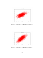
1
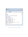
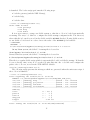
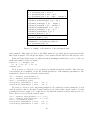
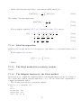
Total sensitivity
Variable X1 =
Variable X2 =
Variable X3 =
index
0.557675
0.442326
0.243721
We now focus on the variance generated by the variables #1 and #3. We set the group
to the empty group with the polychaos_setgroupempty function and add variables with the
polychaos_setgroupaddvar function.
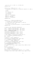
groupe = [1 3];
polychaos_ s e t g r o u p e m p t y ( pc );
pol ychao s_ s e t g r o u p a d d v a r ( pc , groupe (1) );
pol ychao s_ s e t g r o u p a d d v a r ( pc , groupe (2) );
mprintf ( " Fraction of the variance of a group of variables \ n " );
mprintf ( "
Groupe X1 et X2 = %f \ n " , p ol yc h ao s _g et g ro up i nd ( pc ));
The previous script produces the following output.
Fraction of the variance of a group of variables
Groupe X1 et X2 =0.557674
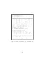
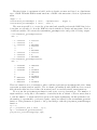
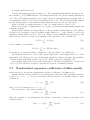
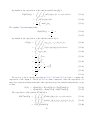
The function polychaos_getanova prints the functionnal decomposition of the normalized
variance.
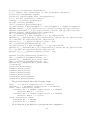
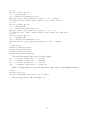
polychaos_getanova ( pc );
The previous script produces the following output.
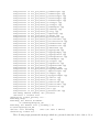
1
0
1
0
1
0
1
0
1
1
0
0
1
1
0
0
0
1
1
1
1
:
:
:
:
:
:
:
0.313953
0.442325
1.55229 e -009
8.08643 e -031
0.243721
7.26213 e -031
1.6007 e -007
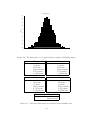
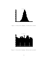
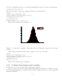
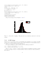
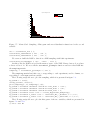
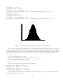
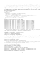
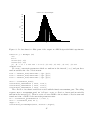
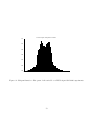
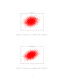
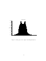
We can compute the density function associated with the output variable of the function. In
order to compute it, we use the polychaos_buildsample function and create a Latin Hypercube
Sampling with 10000 experiments. The polychaos_getsample function allows to quiery the
polynomial and get the outputs. We plot it with the histplot Scilab graphic function, which
produces the figure 6.4.
polychaos_b ui l ds am p le ( pc , " Lhs " ,10000 ,0);
sample_output = polych aos_get sample ( pc );
scf ();
histplot (50 , sample_output )
xtitle ( " Ishigami - Histogram " );
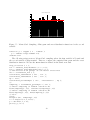
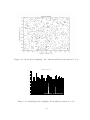
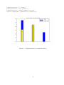
We can plot a bar graph of the sensitivity indices, as presented in figure 6.5.
for i =1: nx
indexfirst ( i )= p o l y c h a o s _ g e t i n d e x f i r s t ( pc , i );
indextotal ( i )= p o l y c h a o s _ g e t i n d e x t o t a l ( pc , i );
end
scf ();
49