1
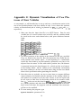
This paper has been mechanically scanned. Some
errors may have been inadvertently introduced.
WSTITUTE OF TRANSPORTATION STUDIES
;UNIVERSITY OF CALIFORNIA, BERKELEY
DYNAVIS: A Dynamic Visualization
Environment for the Design and Evaluation
of Automatic Vehicle Control Systems
A. Kanaris
z. x u
J. Hauser
California PATH
University of California, Berkeley
November 1994
H
PATH TECHNICAL NOTE 94-8
This work was performed as part of the California PATH Program of
the University of California, in cooperation with the State of California Business, Transportation, and Housing Agency, Department of
Transportation; and the United States Department of Transportation,
Federal Highway Administration.
The contents of this report reflect the views of the authors who are
responsible for the facts and the accuracy of the data presented herein.
The contents do no necessarily reflect the official views or policies of
the State of California. This report does not constitute a standard,
specification, or regulation.
DYNAVIS:
A Dynamic Visualization Environment
for the Design and Evaluation
of Automatic Vehicle Control Systems
A. Kanaris, Z. Xu, J. Hauser
Southern California Center for
Advanced Transportation Technologies
EE - Systems, EEB 200B
University of Southern California
Los Angeles, CA 90089-2562
Abstract
DYNAVIS is an interactive engineering environment developed specifically for the
design and evaluation of automatic longitudinal and lateral vehicle control systems.
It can be run on any Silicon Graphics Workstation. The capabilities of DYNAVIS
go far beyond simple animation systems by providing a set of tools to perform interactive visualization with on-line modification of many visualization parameters such
as time and space resolution. The capabilities of this program greatly facilitate detecting undesirable phenomena in automatic vehicle following (platooning), designing
and evaluating vehicle control systems, and comparing the performance of different
control strategies. In this report, we present the desired specifications of a dynamic
visualization system, discuss the issues involved in its design, and describe the dynamic visualization system that we implemented. A user manual has been included
in this report. We anticipate that our dynamic visualization system will be a valuable
tool to designers of automatic vehicle following and platooning systems.
1
Motivation - Conceptual Overview
When we do simulations or experiments, we need an efficient method to analyze
the generated data. For example, consider the simulated or experimental data for a
platoon of four vehicles over a period of five minutes, denoted by T , with sampling
time of 0.1 second, denoted by t,. To study the qualitative characteristics of this
system, one might plot the position, velocity, and possibly acceleration and jerk of
1
each vehicle versus time, 16 plots overall. Because of the high ratio of T / t , and the
lack of an explicit connection between these 16 plots, it will be difficult and time
consuming to understand the nature of the dynamics and to detect the undesirable
system characteristics. In a situation like this, an efficient method is needed to analyze
the data. The dynamic visualization is such a method.
The main idea of dynamic visualization is to take advantage of a humans spatial
intuition. When we see some curves on paper, we may not fully appreciate if the
system behavior is good or not. Some system characteristics may not be visible
by looking at the plots. However, when we see a moving picture, we can easily
recognize the system performance based on our intuition. Thus, by transforming the
numeric data into an animation, we can examine large amount of data with better
comprehension and efficiency. This can be very helpful in the control design and
evaluation. Another reason that makes a dynamic visualization system not only
useful but absolutely essential is the evaluation of system performance under worst
case scenarios. In fact, by employing simulation and dynamic visualization, costly
and dangerous experiments can sometimes be avoided. Next we are going to present
the specifications of this dynamic visualization system and some details about the
methods used.
2
Development of the Specifications
In the development of the dynamic visualization system, we first had to determine the
specifications of the system. We had to decide what needs to be visualized and how to
visualize it. After some study, we focused on a basic set of capabilities that a dynamic
visualization system should have. In this section, we describe these specifications and
discuss the issues involved in the design of a dynamic visualization environment for
automatic vehicle control systems. These specifications have served as the guidelines
during the design phase of the dynamic visualization system.
The dynamic visualization system is required to display the dynamics of individual
vehicles or platoons of vehicles. Therefore the following basic parameters should be
visualized.
Parameters representing the dynamics of individual vehicle namely, position, velocity, acceleration, and jerk.
Parameters directly related to the performance of the controller, such as the desired position of the vehicle and the position error.
Parameters representing the dynamics of the platoon or a group of vehicles, for
example, the string stability.
Parameters directly related to human factor issues, such as the quality of ride,
etc.
2
Typically, we get explicit data for vehicle position and velocity and sometimes
acceleration from the simulations or the experiments. However, data for some other
parameters may not be directly available. Thus, the dynamic visualization system
should include some data processing algorithms to estimate the missing parameters
from the data set provided by the simulation or experiment. For example, jerk data
is not available from simulations in many cases. Since jerk is directly related to the
comfort of passengers and the quality of the ride, it is important to visualize this
parameter. Thus, we must build a post-simulation data processor to estimate the
jerk from position, velocity, and acceleration information.
In order to have a good visualization of all the parameters mentioned above, an
effective user interface is very important. It is one of the major components of the
design of DYNAVIS. It is also one of the main reasons why the dynamic visualization
system is much more advanced than an animation system. When a user uses our
dynamic visualization tool to visualize the dynamics of platoons of vehicles, he should
be able to
0
set up a graphic representation of the static scene, i.e. number of platoons,
number of vehicles per platoon, the parameters to be visualized, etc.,
0 stop at any interesting scene,
run the scene backward and then forward, examining how things lead up to the
situation,
0
review a particular interval of time over and over again,
0 change the time and space resolution arbitrarily.
These interactive user interface abilities provide users with a comprehensive control over when and how to replay a given scene and the ability to home-in on the
precise moment of interest in a timely and effective manner. At the same time, the
user can be hinted by the correlation between various display components for the underlying cause of a given behavior. In fact, without an effective user interface, visual
engineering as discussed above would be an awkward task if one had to change and
compile the program when a certain parameter had to be changed.
To develop this interactive user interface, the programming paradigm had to be
carefully chosen. The development of an environment with the characteristics mentioned above depends heavily on the mode of programming chosen. For example, in
procedural programming with a character-based interface, the application program
is always in control while it is running. In this case, the application allows the user
to give input only at certain pre-specified sections of the program where multiple
levels of menus should be traversed before a certain action can be taken. Clearly this
3
programming paradigm is not suitable for development of a dynamic visualization
environment. In fact an event-driven framework is necessary for this development,
where applications are embedded in an environment which prepares them to respond
to many different events at any time. In this paradigm the user is in control most of
the time. The application starts by setting up a static scene and then enters a loop
from which different functions can be invoked when a designated event is queued.
As mentioned above, an effective user interface should offer users the ability to
change the time resolution arbitrarily. Thus, we should provide an environment which
best brings out the subtleties associated with the dynamics. Since the time resolution
is determined by the time step used in simulations or experiments, in order to increase
the resolution, we have to know the data information at other time instances between
the time interval in the original data. In this case an interpolation technique has to be
used. Employing an interpolation technique is also crucial when the data provided to
the environment has non-uniform time steps. This may happen when automatic step
sizing is used to find the solutions of a set of differential equations by some simulation
software package like Matrix X, Simulink or MATLAB. Furthermore, some time steps
in a non-uniform time step case may be too large to generate real time graphics.
Consequently, without interpolation, visualization would not convey the appropriate
time-dependent properties of the system to the user. The interpolation technique to
be used could be linear, quadratic, or any other nonlinear technique. Using linear
interpolation is well justified when the time step in the original data is small enough,
since parameters of the dynamics of vehicles can be considered to be differentiable,
and differentiability in effect says that locally, parameters change linearly.
To summarize, we have to use an interpolation technique in the dynamic visualization system. By employing this technique and considering the capabilities of
the graphic workstation, the dynamics can then be reviewed in real time or slower or
faster than real time, as chosen by the user. Also it can accept data with non-uniform
time steps.
To help the user better understand the complexity of the dynamics of platoons
of vehicles, the dynamic visualization system must offer the ability to magnify the
behavior of interest. This is another reason why this system is far beyond basic
animation systems. To explain this, let us consider the dynamics of a given vehicle
in a platoon. Assume that this vehicle is automatically controlled, and denote the
position of vehicle i at time t by s ; ( t ) , the desired position of the vehicle by s ; ( t ) ,
A
and the error by e i ( t ) =
si(t) - z;(t). DYNAVIS can be used to visualize e;(t),but
since e i ( t ) may be very small compared to other geometries on the scene, its visual
impact would be limited and detecting its presence may not be easy. Instead, one
can visualize crei(t), where cr is a on-line changeable number, and thus facilitate the
observation of position errors in controller performance, the effects of nonlinearities
or any other relevant system characteristics, with the appropriate resolution.
4
Since DYNAVIS is designed to visualize numeric data describing the dynamics
of vehicle platoons, it mainly accepts and processes data from off-line simulations
and experimental data captured during in-vehicle tests. However, on-line simulation
in DYNAVIS is also desirable. If the dynamic visualization environment has on-line
simulation capability, then the user can interactively specify the speed profile for the
leading vehicle and create various scenarios and disturbances.
The Dynamic Visualization Environment
3
DYNAVIS was developed to aid in the design and evaluation of longitudinal and
lateral vehicle control systems. The current version of the program offers the user the
following capabilities:
0
Visualize the dynamics of one to three platoons with up to ten vehicles in each
platoon. The platoons are displayed side by side. This parallel platoon environment provides a convenient way of comparing the performance of different
control laws. For example we can easily compare the performance of an automatically controlled vehicle platoon to a platoon driven by human drivers. It
also provides a convenient way of comparing the performance of two implementations of the same control law with different controller parameters. DYNAVIS
can easily be reconfigured to visualize one platoon only or two or three platoons
with any number of vehicles, up to ten in each platoon.
0
Visualize each vehicle’s position, velocity, acceleration, and jerk simultaneously.
The position of all the vehicles is displayed graphically on a simulated section
of freeway, with accurate scaling of their positions relative to the freeway lanes
and vehicle size. The velocity of the vehicles can be identified by the relative
velocity of road markers. Provided that the data set contains all the necessary
information, we can also visualize acceleration and jerk. This is done by looking
at the heads of the driver and passenger in each car through the glass sunroof
of the car. The driver holds the steering wheel, so his head is straight during
constant acceleration but it moves if it is subjected to jerk. We assume that the
passenger cannot anticipate any changes in vehicle velocity. The passenger’s
head moves backwards when the vehicle is accelerating and forward when the
vehicle is braking, like a mass suspended from a spring. This assumption allows
us to get a feeling of what it would be like if we were inside the vehicle we are
observing.
For a more accurate reading of vehicle velocity, acceleration and jerk there
are analog and digital meters associated with each vehicle. The position of
the meters is such that identifying the meter corresponding to each vehicle
5
can be done at a glance. The rightmost meter corresponds to the rightmost
vehicle in the platoon. Each analog meter has three pointers, each one of which
corresponds to a car in each lane. The color of the pointer is the same as the
color of the vehicle it corresponds to. This facilitates making quick comparisons
of the performance of the controllers in different lanes of traffic.
0
Evaluate the performance of the controller by indicating the desired position of
each vehicle. The ideal or desired position is a function of the control law chosen
(for example time headway or constant headway). It can be easily changed from
the menu to implement different rules like California safety rule, automatic
control safety distance rule etc.
0
Start, stop and replay the graphic simulation of the platoon dynamics at any
point of interest. The time step is adjustable over a wide range thus allowing
the playback speed to vary from slow motion to fast forward. Frame by frame
advance is also available. The time step of the animation can be changed by
adjusting a slider knob on a logarithmic scale.
The data set does not need to include data points for every frame that can be
displayed. Data sets typically consist of only a few hundred frames and the
time step does not have to be uniform. DYNAVIS can display animations with
apparent resolution of thousands of frames and with any chosen time step. It
achieves that by employing a linear interpolation technique to estimate data for
time instances that fall between existing frames. This in effect can reduce or
increase the speed of animation since DYNAVIS updates the screen at a fixed
frame rate, regardless of the chosen time step. This enhances the illusion of
continuous motion as well as the apparent time resolution.
0
Change the scale by which any position deviations are magnified. When the
controller algorithm is nearly perfect, the position error may become very small.
By magnifying any remaining errors the user can evaluate the performance of
his design and iterate until he is fully satisfied.
0
Interactively modify the zoom factor by selecting the length of the road to be
displayed. This allows the viewer to focus on a section of the platoon instead
of getting an overall "helicopter" view. In the current version of DYNAVIS
we have the leading vehicles appear in fixed positions in each platoon and use
the movement of road markers and the relative motion of the following vehicles
to visualize the changes in vehicle velocity. This enables us to visualize the
platoons with good space resolution.
6
e
Change the spacing between the road markers. This gives the user a reference
point by which he can sense (and even measure) distances with ease unparalleled
in the real world.
e
Change the program configuration by modifying a parameter configuration file.
This file is a plain ASCII file where the user can specify the desired traffic
configuration in terms of number of platoons displayed and number of vehicles
in each platoon. DYNAVIS must be aware of the format of the data file been
supplied to it for visualization. This is achieved by specifying which fields of
information are available from the data file and which fields are not available
but have to be estimated instead. All this information can be specified in the
parameter file, otherwise DYNAVIS will assume some (meaningful) defaults.
The description of the parameter file and the default parameter setup can be
found in the user manual in the Appendix.
In DYNAVIS, the effective user interface is implemented using the
OSF/MOTIF widgets and gadgets. In the current stage of development DYNAVIS
is already equipped with most of the basic functions required by a dynamic visualization system. We have already used it to analyze the dynamics of vehicle platoons.
The data sets came from both simulations and experiments. We have also used it
to evaluate vehicle control laws and had some very useful results. For example we
have used it to compare two automatic control laws. One control law was using
acceleration information from the leading vehicle, and the other did not use this information. By monitoring the position, speed, acceleration, and jerk, we easily found
that both controllers achieve similar position and speed performance, but the one
without knowledge of the leading vehicle’s acceleration resulted in smaller jerk.
These actual application tests show that dynamic visualization is a very useful tool
for the analysis of the complex and highly coupled dynamics of vehicle platoons. In the
future, we anticipate using these and other forthcoming enhancements in DYNAVIS
to design even better controllers for vehicle platoons.
4
Desirable Enhancements
We have thought of many further enhancements that are possible for DYNAVIS which
will make the environment a more powerful and flexible tool.
0 Enhance the support for lane change maneuvers, through the already avail-
able lateral position specification. The objective is to allow the user to better
visualize the lateral dynamics of the vehicles during lane changes.
7
0
Devise a mechanism to obtain acceleration and jerk information for purpose of
visualization when the data set does not provide such information. This may
be achieved by appropriate filtering of available vehicle data.
0
Enhance user friendliness and interaction by adding help screens, parameter
input menus and dialog boxes.
0
Add MAX and MIN memory capability to the meters. Extra pointers on the
meters can indicate the maximum and minimum data value reached during a
visualization session. The feature can be turned on and off by a radio button
selection.
0
Add the ability to set the limits (beginning and end) of a time period of interest and repeat this interval over and over again to allow the user to choose
different speeds and magnification to study a particularly interesting portion of
the animation. Currently the user has to pull back the Time Index slider knob
every time he wants to review a specific time period.
0
Address some human factor issues in the visualization, such as devising indicators for the comfort level and quality of the ride and some appropriate means
of displaying them.
0
Provide some means of choosing interactively the scenarios for visualization.
The user should be able to specify and load a new data file at any time during
a visualization session without having to stop and reload DYNAVIS.
CI
Make the visualization environment three dimensional, with provision to specify
the viewpoint and the viewport. Extend the system with “scenery” files in order
to allow for the highway to have turns and uphill and downhill sections. Extend
the format of the data files to include vehicle position in the vertical direction.
0 Study the possibility of integrating some limited simulation capabilities in the
visualization environment and its negative impact on visualization speed and
flexibility.
Appendix A:
DYNAVIS User Manual
Make sure that dynavis, the current version of DYNAVIS is in your current path or
directory and start execution by typing:
dynavis dataf i l e parameterf i l e
8
The first argument is the user supplied data file. If it is not provided dynavis will
refuse to run and instead will print the correct syntax for invoking DYNAVIS.
The second argument is the name of the optional but recommended parameter
configuration file.
The data file provides all the position, velocity, acceleration and jerk information
for each vehicle in each time step. All the data for a single time step has to be
in one line, since the program searches for the newline character to parse the data
file. The first item on each line must be the current time step value, followed by
the data fields. The only delimiter allowed between data is one or more spaces. The
visualization program makes very few assumptions about the data itself.
The parameter file is not strictly required but it is preferable to have all the parameters specified when DYNAVIS is started. The format of the parameter configuration
file can be seen in this example:
Platoons= 2
Cars= 4
Relative= 0
PositionX= 1
Position-Y= 0
VelocityX= 1
Velocity-Y= 0
Accelavail= 1
Jerkavail= 1
The values we used in the example happen to be the default values assumed by
DYNAVIS if the parameter file is not supplied in the command line. These values
will also be used in the case that any one of the parameters is not specified in the
parameter file. The syntax rules are very simple: The parameter name has to be at
the beginning of a line, followed by an equal sign followed by a space and an integer
value.
The variable “Platoons” specifies the number of platoons of vehicles in the range
one to three.
The variable “Cars” allows the number of vehicles in each platoon to be specified
in the range one to ten.
The position of each vehicle may be specified as the absolute distance traveled
from the beginning of the simulation or as a relative distance between vehicles. The
variable Relative should be set to 1if the file contains relative distances or 0 otherwise.
The availability of a number of state variables such as X-axis position Y-axis
position, X-axis velocity, Y-axis velocity, acceleration and jerk has to be specified
in order to match the format of the supplied data file. This is done by setting a
parameter value equal to 1 if the parameter is available in the data file and 0 if there
is no corresponding field in the data file.
9
Appendix B: Dynamic Visualization of Two Platoons of Four Vehicles
As an example, we will describe how to set up and run a visualization session in the
case of two parallel platoons with four vehicles in each. Let us denote the position,
velocity, acceleration and jerk of vehicle j in platoon i by pos;j, vel;j, acc;j and j r k i j ,
respectively.
1. Make sure that the input data file is in ASCII format. Data for each
variable has to be stored column wise in the file, and the variables should
be saved in the exact order shown below, with space delimiters between
fields.
time
posx11 POSY11 vel11 aCCll j r h l
~ 0 ~ x posy12
12
vel12 acc12 .irk12
posx13 posy13 vel13 acc13 j r h
posx14 posy14 vel14 acc14 jrk14
posx22 posy22 vel22 ace22 jrk22
posx23 posy23 vel23 ace23 jrk23
posxz4 p0sy2~vel24 ace24 jrk24 newline character (OxOA)
2. The initial positions of the vehicles in the platoons are not pre- specified.
They are found in the data file. But the parameters that define the desired positions have default values. At the beginning of a visualization
session the time headway and fixed headway parameters may have to be
adjusted from the menu. In files with relative position data, the distance
is measured between the front bumper of a vehicle and the rear bumper
of the leading vehicle. All the vehicles in the visualization environment
have been assumed to be four and a half meters long and the user should
observe this specification when generating the data file.
3. Note that since we typically use two or more lanes to compare different
control schemes, the position and the dynamics of the leading vehicles in
each platoon are assumed to be the same. Hence we do not require and
do not expect to find data for the leading vehicle in the second or third
jrk21 ~ 0 ~ x 3
veZgl
1
lane. (i.e. we do not save the data for ~ 0 ~ x 2 1
etc.). If the positions and other data for the leading vehicles in the other
lanes are not the same, the program code and associated data structures
will have to be modified.
4. To start running the program, type
dynavis dataf i l e parameterf i l e
10
at the UNIX prompt. After a few seconds the outline of a window will
appear. Use the mouse to move the outline window to any point on the
screen. Click the left mouse button to open the window at the desired
position. Use the middle button to adjust the window’s position after it
is opened. At this point you should see the initial scene of a section of
highway and the vehicles on it, along with the meters corresponding to
each vehicle. The top row of meters indicate velocities. Colored needles
in the meters (Red, green, and blue) correspond to the cars of the same
color. The middle row of meters indicate acceleration and the bottom row
of meters indicate the jerk.
5. To stop the program, move the mouse pointer to the menu section and
click on the “Command” option, then highlight “Stop” and release. The
vehicles and the meters will freeze.
6. To restart the animation, move the mouse pointer to the menu section,
click the “Command” option, highlight “Start” and release the button.
7. Use the scales at the bottom of the window to adjust the time step (speed
of animation), shuttle to another point in time, change the road length
(zoom factor), magnify the position errors, change the spacing between
the road markers.
8. To exit from DYNAVIS go back to the menu and choose the “Quit))option
under the “Command)’ menu.
Appendix C: Video Tape Demonstration
We have created a video tape which shows an overview of the capabilities of the
current version of dynamic environment and a sample session of using and interacting
with DYNAVIS. For a copy of this video tape please contact the authors at the
University of Southern California, Center for Advanced Transportation Technologies.
11