1
TASPLAQ v2.x
User Manual
TASPLAQ module
B. User Manual
1. SIGN NOTATIONS AND CONVENTIONS ..................................................................................... 3 1.1 SIGN NOTATIONS AND CONVENTIONS ........................................................................................... 3 1.2 UNITS ........................................................................................................................................ 3 2. GLOBAL PRESENTATION OF THE USER INTERFACE ............................................................. 4 3. DATA INPUT ................................................................................................................................... 5 3.1 GENERAL OPERATION OF DATA INPUT .......................................................................................... 5 3.2 GENERAL SETTINGS .................................................................................................................... 6 3.2.1 Calculation settings ............................................................................................................ 6 3.2.2 Elastic thresholds for soil-plate interaction ........................................................................ 6 3.2.3 Geometry dimensions ........................................................................................................ 7 3.3 DEFINING THE LAYERS .............................................................................................................. 10 3.4 MESH ALONG X-AXIS ................................................................................................................. 12 3.5 MESH ALONG Y-AXIS ................................................................................................................. 14 3.6 DEACTIVATING ELEMENTS ......................................................................................................... 16 3.7 DEFINING THE MECHANICAL PROPERTIES OF THE PLATE .............................................................. 19 3.8 DEFINING THE LOAD DISTRIBUTED ON THE PLATE ........................................................................ 21 3.9 DEFINING LOAD ON NODES ........................................................................................................ 24 3.10 DEFINING EXTERNAL LOADS APPLIED TO THE SOIL ...................................................................... 26 3.11 MANUAL CONTROL OF SEPARATED AND PLASTIC NODES (OPTIONAL) ............................................ 28 4. CALCULATIONS........................................................................................................................... 30 5. RESULTS ...................................................................................................................................... 32 5.1 5.2 5.3 5.4 5.5 5.6 6. RESULT FILE............................................................................................................................. 32 EXPORT TO A NEW SPREADSHEET ............................................................................................. 33 CROSS SECTIONS ..................................................................................................................... 34 2D SCATTER POINTS ................................................................................................................. 35 3D GRAPH WIZARD ................................................................................................................... 35 DEHOMOGENISATION ................................................................................................................ 36 INPUT AND OUTPUT FILES ........................................................................................................ 38 6.1 INPUT: CONSTITUTION OF THE INPUT DATA FILE (TPL)............................................................... 38 6.2 OUTPUT FILES .......................................................................................................................... 40 6.2.1 Result file ......................................................................................................................... 40 6.2.2 TASSELDO file ................................................................................................................ 41 6.2.3 Influence matrix temporary backup file ............................................................................ 41 6.2.4 File for use under Microsoft Excel®.................................................................................. 41 Copyright TASPLAQ / FOXTA v3 - TERRASOL - August 2009 - Ind 0
Page 1 / 41
TASPLAQ v2.x
User Manual
LIST OF FIGURES
FIGURE 1: HOME PAGE OF TASPLAQ INPUT ............................................................................................................ 4 FIGURE 2: GENERAL PARAMETERS - EXAMPLE ...................................................................................................... 8 FIGURE 3: DEFINITION OF GEOMETRY DIMENSIONS ............................................................................................... 9 FIGURE 4: WORK COORDINATE SYSTEM ................................................................................................................. 9 FIGURE 5: LAYER DEFINITION ............................................................................................................................... 10 FIGURE 6: EXAMPLE OF LAYERS DEFINITION ........................................................................................................ 11 FIGURE7: MESH ALONG X-AXIS – MODELLING PRINCIPLES ................................................................................. 12 FIGURE 8: EXAMPLE OF MESH ALONG X-AXIS ...................................................................................................... 13 FIGURE 9: MESH ALONG Y-AXIS – MODELLING PRINCIPLES ................................................................................ 14 FIGURE 10: EXAMPLE OF MESH ALONG Y-AXIS .................................................................................................... 15 FIGURE 11: GLOBAL MESH ................................................................................................................................... 16 FIGURE 12: ELEMENT DEACTIVATION TECHNIQUE ............................................................................................... 17 FIGURE 13: ELEMENTS DEACTIVATED (EXAMPLE) ............................................................................................... 17 FIGURE 14: EXAMPLE OF ELEMENT DEACTIVATION.............................................................................................. 18 FIGURE 15: EXAMPLE OF DEFINITION OF THE MECHANICAL PROPERTIES OF THE PLATE .................................... 20 FIGURE 16: COMBINED SECTION CALCULATION ................................................................................................... 21 FIGURE 17: EXAMPLE OF LOAD DISTRIBUTED ON THE PLATE .............................................................................. 23 FIGURE 18: EXAMPLE OF POINT LOAD .................................................................................................................. 25 FIGURE 19: GLOBAL LAYOUT OF THE PROBLEM {PLATE + SOIL + EXTERNAL LOADS} ........................................ 26 FIGURE 20: COORDINATES OF EXTERNAL LOADS ................................................................................................ 26 FIGURE 21: EXAMPLE OF EXTERNAL LOADS ON THE SOIL.................................................................................... 27 FIGURE 22: MANUAL DEFINITION OF NODE SEPARATION / PLASTIFICATION - EXAMPLE ....................................... 28 FIGURE 23: HOMEPAGE OF TASPLAQ INPUT......................................................................................................... 30 FIGURE 24: CALCULATION WINDOW...................................................................................................................... 31 FIGURE 25: HOME PAGE OF TASPLAQ OUTPUT .................................................................................................... 32 FIGURE 26: *.RESU FILE - EXAMPLE ..................................................................................................................... 33 FIGURE 27: EXPORTING THE FILE UNDER MICROSOFT EXCEL® ......................................................................... 33 FIGURE 28: SETTLEMENT ALONG X IN Y = 5 AND Y = 7 ...................................................................................... 34 FIGURE 29: 2D SCATTER POINTS ......................................................................................................................... 35 FIGURE 30: HOME WINDOW OF TASPLAQ GRAPHIQUE3D.XLS ........................................................................ 35 FIGURE 31: 3D GRAPH WINDOW .......................................................................................................................... 36 FIGURE 32: HOME WINDOW OF TASPLAQ DESHOMOGENISATION.XLS ............................................................. 36 FIGURE 33: WINDOW [CHARACTERISTICS OF THE LOWER LAYER] ...................................................................... 37 FIGURE 34: DEHOMOGENISATION ........................................................................................................................ 37 LIST OF TABLES
TABLE 1: SIGN NOTATIONS AND CONVENTIONS ..................................................................................................... 3 TABLE 2: UNITS ....................................................................................................................................................... 3 TABLE 3: SUMMARY OF GENERAL SETTINGS .......................................................................................................... 9 TABLE 4: SUMMARY OF PARAMETERS REQUIRED FOR SOIL DEFINITION .............................................................. 10 TABLE 5: PARAMETERS REQUIRED TO DEFINE MESH ALONG X-AXIS ................................................................... 12 TABLE 6: DEACTIVATION PARAMETERS ................................................................................................................ 16 TABLE 7: PARAMETERS FOR ALLOCATING MECHANICAL CHARACTERISTICS ....................................................... 19 TABLE 8: PARAMETERS FOR DISTRIBUTED LOAD ................................................................................................. 22 TABLE 9: PARAMETERS FOR LOADS ON NODES ................................................................................................... 24 TABLE 10: SETTING OF EXTERNAL LOADS ON THE SOIL....................................................................................... 28 TABLE 11: PARAMETERS FOR MANUAL SEPARATION/PLASTIFICATION MANAGEMENT......................................... 29 Page 2 / 41
Copyright TASPLAQ / FOXTA v3 - TERRASOL - August 2009 - Ind 0
TASPLAQ v2.x
User Manual
1. SIGN NOTATIONS AND CONVENTIONS
1.1
Sign notations and conventions
Magnitude
Rotations and moments
Plate deflection
Soil settlement
Shear forces
Representation
M x , M y , M xy
x , y , p , r
w
Tass
Tx , T y
Sign convention
Trigonometric meaning
Positive downwards
Positive downwards
Positive upwards
Positive downwards
Springs
q, Fz
ps
C x , C y , K z , Ks z
Loads
x , y , xy
Positive in traction
Vertical load (distributed or point)
Soil reaction, interaction pressure
Positive upwards
Always positive
Table 1: Sign notations and conventions
1.2
Units
Magnitude
Lengths and coordinates
Vertical point load Fz
Moments (Mx, My, Mxy)
Shear forces (Tx, Ty)
Soil reaction, distributed loads
Displacements (deflection w, settlement s)
Rotations
Young’s modulus E
Distributed springs / subgrade reaction
Linear springs
Rotation springs
Unit
m
kN
kN.m/ml
kN/ml
kPa
m
rad
kPa
kPa/m
kN/m
kN.m/rad
Table 2: Units
Copyright TASPLAQ / FOXTA v3 - TERRASOL - August 2009 - Ind 0
Page 3 / 41
TASPLAQ v2.x
User Manual
2. GLOBAL PRESENTATION OF THE USER INTERFACE
The application’s interface was developed under Microsoft Excel®. When opening the
TASPLAQ_vx.x.xls file, a home page appears (Figure 1).
It allows to select an existing file or create a new one. The work directory can also be
configured.
The installation directory is entered automatically.
From this interface, you can:
Access data entry ([Start modelling]) ;
Launch the calculation: the interface then calls upon TASPLAQ’s calculation engine
to run the .tpl file created during modelling ;
Display results: the calculation results are accessible from the TASPLAQ
Output_vx.x.xls file (Microsoft Excel®).
Figure 1: home page of Tasplaq input
Page 4 / 41
Copyright TASPLAQ / FOXTA v3 - TERRASOL - August 2009 - Ind 0
TASPLAQ v2.x
User Manual
3. DATA INPUT
To access data input or modification press the [Start modelling] button.
3.1
General operation of data input
Data input is performed by following the steps described in the next paragraphs. These steps
correspond to the different types of data to be defined.
This input is accompanied with graphic viewing updated automatically when adding
information.
Screenshots of the application illustrate each of the steps in making the model.
Once the TASPLAQ_vx.x.xls file is open, you can either create a new calculation file, or open
an existing file.
To create a new calculation file:
Click the [New project] button, a new window opens.
Enter the name of the file to create.
Click the [Browse…] button to choose
the work directory to save the *.tpl file.
The installation directory is configured
automatically.
Click the [Validate] button to return to
the home page.
To open an existing calculation file:
Click the [Open a TASPLAQ file] button, a new window opens.
Choose the directory containing the
*.tpl file required.
Select the file, then click the [Open]
button.
Click the [Start modelling] button to input your data.
Copyright TASPLAQ / FOXTA v3 - TERRASOL - August 2009 - Ind 0
Page 5 / 41
TASPLAQ v2.x
User Manual
Data is entered in the module using 9 tabs filled successively. Move between the tabs using
the [Next] and [Previous] buttons. We recommend following the tab sequence.
Once data has been input in the 9 tabs, a window opens to save a data file in the .tpl format.
The content of this file is explained in paragraph 6.
3.2
General settings
The following are the general settings to be entered.
3.2.1 Calculation settings
Import stiffness matrices: allows importing the influence matrix of a previous
calculation, presumably saved beforehand. It ensures a major time gain in the case of
a system with several loading cases.
Save stiffness matrices: used to save the soil influence matrix for a subsequent
calculation. This option is used in the case of a system with several loading cases for
example.
Automatic control: allows automatic consideration of separation and/or plastification
to points as per the separation and plastification criteria defined in the section
‘thresholds for soil-plate interface‘.
Symmetries: allows considering symmetries, along x-axis or/and along y-axis.
Printing content: controls printing of the results file. This choice is related only with
the data summary: Reduced print = short summary of the data / Detailed printing =
detailed summary of the data.
3.2.2 Elastic thresholds for soil-plate interaction
These parameters concern surface soil only. They intervene in the calculation only in the
case of a plate on supporting soil, and only if automatic calculation has been requested.
Separation threshold (kPa): limit stress in traction at the Soil-Plate interface,
beyond which the corresponding points are considered as being ‘separated’. Soil
reaction beside these points is hence zero, and there is no longer equality between
soil settlement and the vertical displacement of the plate.
Plastification threshold (kPa): limit stress in compression at the Soil-Plate
interface, beyond which the corresponding points are considered as being ‘plastified’.
The soil’s reaction beside these points is imposed (equal to the plastification
threshold), but equality between soil settlement and vertical displacement of the plate
is always ensured.
Page 6 / 41
Copyright TASPLAQ / FOXTA v3 - TERRASOL - August 2009 - Ind 0
TASPLAQ v2.x
User Manual
3.2.3 Geometry dimensions
This means defining the local coordinate system of the plate. Therefore, the general case
includes two coordinate systems:
A reference coordinate system O0 x0 , O0 y 0 , O0 z 0 , containing the plate as well as the
external loads applied directly to the soil.
A local coordinate system Ox, Oy, Oz associated with the plate, defining the mesh,
as well as different characteristics. This coordinate system is such that the plane
Ox, Oy is parallel to O0 x0 , O0 y 0 . Hence it can be defined perfectly using two
parameters:
o The coordinates
x p , y p , z p of point
O in the reference coordinate system.
Beware! Zp is the reference level of the project.
o The rotation angle p of the axis Ox in respect of the O0 x0 axis.
Copyright TASPLAQ / FOXTA v3 - TERRASOL - August 2009 - Ind 0
Page 7 / 41
TASPLAQ v2.x
User Manual
Figure 2: General parameters - example
Page 8 / 41
Copyright TASPLAQ / FOXTA v3 - TERRASOL - August 2009 - Ind 0
TASPLAQ v2.x
User Manual
Y-axis
Geometry
dimensions
LXmax
Plate
LYmax
Ymin
X-axis
Xmin
Figure 3: definition of geometry dimensions
O0 y 0
O0 z 0
top view
Oy
Ox
zp
plate
Ox
O
O0 x 0
O0
p
yp
O
xp
vertical cross-section
O0
O0 x 0
xp
Figure 4: work coordinate system
Designation
Display condition
Mandatory
value
Unit
Default value
None
Unchecked
Always
Yes
Import stiffness
matrices
Save stiffness
matrices
Automatic control
Symmetries
None
Unchecked
Always
Yes
None
None
Always
Always
Yes
Yes
Printing content
None
Always
Yes
kPa
Unchecked
No symmetries
Detailed
printing
5
Always
Yes
kPa
10000
Always
Yes
XP
m
0
YP
m
0
ZP
m
0
Theta
°
0
Separation threshold
Plastification
threshold
Only if there are no more
symmetries. Otherwise, value set
to 0 (no modification possible)
Only if there are no more
symmetries. Otherwise, value set
to 0 (no modification possible)
Always
Only if there are no more
symmetries. Otherwise, value set
to 0 (no modification possible)
Yes
Yes
Yes
Yes
Table 3: summary of general settings
Copyright TASPLAQ / FOXTA v3 - TERRASOL - August 2009 - Ind 0
Page 9 / 41
TASPLAQ v2.x
User Manual
3.3
Defining the layers
The soil is made of a series of horizontal layers, each characterised by its Young’s modulus,
its Poisson’s ratio and the level of its base. Hence, the ‘i’ layer is located between the
z z i 1 and z z i planes. Conventionally, we take z 0 equal to z p , level of the plate
(Figure 5).
Plate
Oz
z=Z0
E1, 1
z=z1
E 2, 2
z=z2
E 3, 3
z=z3
Figure 5: Layer definition
The following figure details the parameters required to define the layers. The user can view
the layout of the layers in the form of a vertical cross-section. In this diagram, the soil’s
surface is taken equal to the level of the ZP plate defined in general settings.
This step is not mandatory: e.g. in the case of a calculation on elastic supports only, no soil
layers are defined.
The table below summarises the layer definition parameters:
For each layer,
enter:
Enter once
None
Value
by default
---
Condition
of display
Always
Mandatory
value
No
m
---
Always
Yes
kPa
---
Always
Yes
None
---
Always
Yes
kPa
0
Always
Yes
Designation
Unit
Layer name
Level of the base of
the layer
Young’s modulus of
the layer
Poisson’s ratio
Initial vertical stress
on surface
Table 4: summary of parameters required for soil definition
Page 10 / 41
Copyright TASPLAQ / FOXTA v3 - TERRASOL - August 2009 - Ind 0
TASPLAQ v2.x
User Manual
Figure 6: Example of layers definition
Copyright TASPLAQ / FOXTA v3 - TERRASOL - August 2009 - Ind 0
Page 11 / 41
TASPLAQ v2.x
User Manual
3.4
Mesh along x-axis
We then go to the local coordinate system of the plate. The mesh is defined in two steps
corresponding to the x-axis and y-axis directions. At first, we look at the mesh along x-axis.
The plate is divided into one or several clusters along the x-axis. Each cluster is
characterised by its length Lx(i) and associated number of subdivisions Nx(i) as shown in the
diagram below.
This step is mandatory, at least one cluster must be defined.
LXmax
LYmax
Length=Lx(2)
Nx(2)=3
Length=Lx(1)
Nx(1)=4
Length=Lx(3)
Nx(3)=1
Length=Lx(4)
Nx(4)=2
Figure7: Mesh along x-axis – Modelling principles
In the graphic window, the plate is shown by a top view: the user can view the discretization
defined upon entry.
The table below summarises the parameters required:
Designation
Length of the
cluster
Number of
subdivisions
Unit
Default value
Display
condition
Mandatory value
m
---
Always
Yes
None
---
Always
Yes
Table 5: Parameters required to define mesh along x-axis
Page 12 / 41
Copyright TASPLAQ / FOXTA v3 - TERRASOL - August 2009 - Ind 0
TASPLAQ v2.x
User Manual
Figure 8: Example of mesh along x-axis
Copyright TASPLAQ / FOXTA v3 - TERRASOL - August 2009 - Ind 0
Page 13 / 41
TASPLAQ v2.x
User Manual
3.5
Mesh along y-axis
As the mesh is defined along the x-axis direction, a discretization along y-axis is
superimposed according to the same principle, as shown in the figure below.
This step is mandatory, at least one cluster must be defined.
LXmax
Length=Ly(4)
Ny(4)=1
Length=Ly(3)
Ny(3)=3
LYmax
Length=Ly(2)
Ny(2)=1
Length=Ly(1)
Ny(1)=3
Figure 9: Mesh along y-axis – Modelling principles
The principle of discretization is identical to that considered for the x-axis direction: the pitch
is defined by cluster, each cluster being characterised by its length Ly(i) and the associated
number of subdivisions Ny(i) as shown in the diagram above.
Caution! The total number of Nx Ny elements must be below 2500 (maximum manageable
by Windows environment).
Page 14 / 41
Copyright TASPLAQ / FOXTA v3 - TERRASOL - August 2009 - Ind 0
TASPLAQ v2.x
User Manual
Figure 10: Example of mesh along y-axis
Superimposing the two x-axis and y-axis meshes leads to the final mesh.
Copyright TASPLAQ / FOXTA v3 - TERRASOL - August 2009 - Ind 0
Page 15 / 41
TASPLAQ v2.x
User Manual
LXmax
LYmax
Figure 11: Global mesh
3.6
Deactivating elements
Once the mesh has been defined, the ‘effective’ plate geometry must be set. Indeed,
complex plate geometries can be modelled, using the element deactivation option.
This step is not mandatory: if no element is deactivated, the plate is assumed to cover the
entire mesh.
Each deactivated cluster of the plate is defined by a group of elements corresponding to a
rectangular cluster.
The groups of elements themselves are defined using a numbering system: elements are
numbered in each direction to facilitate group selection in the form ‘i1 i2 j1 j2‘.
Note: the element numbering system in each direction appears in Figure 13.
The following table lists the parameters required:
Designation
Unit
Value
by
default
Condition
of display
Mandatory
value
i1*
None
---
Always
Yes
i2*
None
---
Always
Yes
j1*
None
---
Always
Yes
j2*
None
---
Always
Yes
Local checks
>0 and <= total number of
subdivisions along x-axis
>=i1 and <= total number of
subdivisions along x-axis
>0 and <= total number of
subdivisions along (y-axis)
>=j1 and <= total number of
subdivisions along x-axis
*: i1, i2, j1 and j2 are the basic coordinates of the deactivated cluster (Figure 13)
Table 6: Deactivation parameters
One or several clusters can be deactivated.
The clusters deactivated are outlined by a red line in the drawing.
Page 16 / 41
Copyright TASPLAQ / FOXTA v3 - TERRASOL - August 2009 - Ind 0
TASPLAQ v2.x
User Manual
The following figures show a few possible cases.
Y-axis
Deactivated
element
Activated
element
X-axis
Figure 12: Element deactivation technique
1 2
3
4
5
i1=6
7
i2=8
9
j2=4
j1=3
2
1
In white deactivated elements cluster (6 8 3 4)
Figure 13: Elements deactivated (example)
Copyright TASPLAQ / FOXTA v3 - TERRASOL - August 2009 - Ind 0
Page 17 / 41
TASPLAQ v2.x
User Manual
i1 = 9, i2 = 9, j1 = 1 et j2 = 17
Figure 14: Example of element deactivation
Page 18 / 41
Copyright TASPLAQ / FOXTA v3 - TERRASOL - August 2009 - Ind 0
TASPLAQ v2.x
User Manual
3.7
Defining the mechanical properties of the plate
The properties of the plate are presumed uniform for each element. Each element is
characterised by its Young’s modulus ‘E’, its ‘bare’ Poisson’s ratio, as well as its thickness
‘h’. This data can be assigned by groups of elements. The allocation principle is identical to
that used for deactivating elements: i.e. allocation by groups of elements.
This step is mandatory. At least one cluster must be defined in the case of a plate with
homogeneous characteristics.
Here again we use group definitions of the ‘i1 i2 j1 j2’ type.
The clusters created are outlined by a red line in the graph of the application.
When defining a small cluster with different characteristics inside a larger cluster, first define
the larger cluster, then the smaller cluster with its different characteristics. The characteristics
of the small cluster ‘overwrite’ and replace those defined previously.
The table below summarises the parameters to enter:
Designation
Unit
Value
by
default
i1
None
---
Always
Yes
i2
None
---
Always
Yes
j1
None
---
Always
Yes
j2
None
---
Always
Yes
---
Always
Yes
>0
-----
Always
Always
Yes
Yes
>0 and < 0.5
>0
Young’s
modulus of the kPa
plate
Poisson’s ratio
None
Plate thickness
m
Condition
of display
Mandatory
value
Local checks
>0 and <= Total number of
subdivisions along x-axis
>=i1 and <= Total number of
subdivisions along x-axis
>0 and <= Total number of
subdivisions along (y-axis)
>=j1 and <= Total number of
subdivisions along x-axis
Table 7: Parameters for allocating mechanical characteristics
Copyright TASPLAQ / FOXTA v3 - TERRASOL - August 2009 - Ind 0
Page 19 / 41
TASPLAQ v2.x
User Manual
Figure 15: Example of definition of the mechanical properties of the plate
Page 20 / 41
Copyright TASPLAQ / FOXTA v3 - TERRASOL - August 2009 - Ind 0
TASPLAQ v2.x
User Manual
The ‘Calculation wizard for combined section’ button starts the wizard for calculating a
combined section using the data to be entered as shown in the figure below.
Figure 16: combined section calculation
This wizard allows defining equivalent mechanical properties or what can be called
‘homogenised parameters’, if the plate section is not homogeneous. Please note that the use
of this technique may be ‘useful’ in certain specific cases, as the one described in tutorial 8.
3.8
Defining the load distributed on the plate
This tab allows defining one or several loads distributed over the plate, as well as any one or
several distributed springs under the plate. As previously, this load is defined by groups of
elements.
This step is not mandatory.
Copyright TASPLAQ / FOXTA v3 - TERRASOL - August 2009 - Ind 0
Page 21 / 41
TASPLAQ v2.x
User Manual
Designation
Unit
Value
by
default
Condition
of display
Mandatory
value
i1
None
---
Always
Yes
i2
None
---
Always
Yes
j1
None
---
Always
Yes
j2
None
---
Always
Yes
---
Always
Yes
---
---
Always
Yes
Positive
Load distributed
vertically on the
kPa
plate
Springs*
kPa/m
Local checks
>0 and <= total number
of subdivisions along
x-axis
>=i1 and <= total
number of subdivisions
along x-axis
>0 and <= total number
of subdivisions along
(y-axis)
>=j1 and <= total
number of subdivisions
along x-axis
*: stiffness distributed in displacement under the plate, for example representative of a distribution of
juxtaposed springs
Table 8: Parameters for distributed load
If several loads are defined over the same cluster, they are added. The operation is the same
for springs.
Page 22 / 41
Copyright TASPLAQ / FOXTA v3 - TERRASOL - August 2009 - Ind 0
TASPLAQ v2.x
User Manual
Figure 17: Example of load distributed on the plate
Copyright TASPLAQ / FOXTA v3 - TERRASOL - August 2009 - Ind 0
Page 23 / 41
TASPLAQ v2.x
User Manual
3.9
Defining load on nodes
Each load on nodes is made of a vertical load, two bending moments, one spring in
translation, two springs in rotation. This data is assigned by groups of nodes. Each is defined
using nodes with maximum/minimum index. The principle for each group’s coordinates is
similar to that used for groups of elements.
The values entered apply to each of the nodes in the cluster.
This step is not mandatory.
The table below summarises the parameters to enter:
Designation
Unit
Value
by default
Condition
of display
Mandatory
value
Local checks
i1
None
---
Always
Yes
i2
None
---
Always
Yes
j1
None
---
Always
Yes
j2
None
---
Always
Yes
kN
---
Always
Yes
>0 and <= total
number of
subdivisions along
x-axis + 1
>=i1 and <= total
number of
subdivisions along
x-axis +1
>0 and <= total
number of
subdivisions along
y-axis +1
>=j1 and <= total
number of
subdivisions along
x-axis +1
---
kN.m
---
Always
Yes
---
kN.m
---
Always
Yes
---
kN/m
---
Always
Yes
Positive
---
Always
Yes
Positive
---
Always
Yes
Positive
Unchecked
Always
---
Fz (vertical point load)
Mx (moment around the
y-axis)
My (moment around the
x-axis)
Kz (linear spring under
the plate)
Cx (rotation spring
around the y-axis)
Cy (rotation spring
around the x-axis)
Manual management of
Node
Separation/Plastification
kN.m/
rad
kN.m/
rad
---
The number of soil
layers must be
positive
Table 9: Parameters for loads on nodes
The ‘Manual control of separated and plastic points’ option allows the user to define manually
the nodes to declare as separated or plastified. In this case, a new tab ‘nodes to separate /
plastify‘ appears (see § 3.11).
Page 24 / 41
Copyright TASPLAQ / FOXTA v3 - TERRASOL - August 2009 - Ind 0
TASPLAQ v2.x
User Manual
Figure 18: Example of point load
Copyright TASPLAQ / FOXTA v3 - TERRASOL - August 2009 - Ind 0
Page 25 / 41
TASPLAQ v2.x
User Manual
3.10
Defining external loads applied to the soil
In addition to pressure applied by the plate, the soil may be subject to ‘direct’ external loads.
These loads are presumed rectangular shaped, positioned and turned in the global
coordinate system.
The following figure describes the global position of the problem:
Plate
External loads on the
plate
External loads on the soil
Figure 19: Global layout of the problem {Plate + Soil + External loads}
Each load is characterised by the coordinates of its ‘lower – left’ top
(Xr, Yr, Zr), dimensions (DLX width and DLY length), orientation (θr), as well as its load (qr).
Oy
Plate
External load
p
yp
r
yr
Ox
xp
xr
Figure 20: Coordinates of external loads
Tasplaq proposes a top view of these loads, as well as of the plate. We can note that the
external loads are not always oriented in parallel with the x-axis and y-axis axes (Figure 20):
they can be placed with any angle in respect of these axes.
This step is not mandatory.
Page 26 / 41
Copyright TASPLAQ / FOXTA v3 - TERRASOL - August 2009 - Ind 0
TASPLAQ v2.x
User Manual
Figure 21: Example of external loads on the soil
Copyright TASPLAQ / FOXTA v3 - TERRASOL - August 2009 - Ind 0
Page 27 / 41
TASPLAQ v2.x
User Manual
Designation
Unit
XR
YR
ZR
DLX
DLY
Theta
qr
m
m
m
m
m
°
kPa
Value
by default
---------------
Condition
of display
Always
Always
Always
Always
Always
Always
Always
Mandatory
value
Yes
Yes
Yes
Yes
Yes
Yes
Yes
Local
checks
------>0
>0
-----
Table 10: Setting of external loads on the soil.
3.11
Manual control of separated and plastic nodes (optional)
This button allows to impose the following manually:
Separation of certain nodes: the soil’s reaction then equals 0 and soil settlement no
longer equals the vertical displacement of the plate.
Plastification of certain nodes: the soil’s reaction imposed equals the plastification
threshold defined in ‘general settings’. Equality between soil settlement and the
vertical displacement of the plate is always ensured.
The ‘separation/plastification manual management’ can be combined with the ‘automatic
calculation’: Indeed, if the ‘automatic calculation’ option is activated, TASPLAQ checks
separation/plastification beside all nodes, except those declared separated/plastified
manually by the user.
This option corresponds to an advanced use of Tasplaq.
Figure 22: manual definition of node separation / plastification - example
If this option is not activated, the number of nodes separated and plastified is reset to zero.
Of course, this step is not mandatory.
Page 28 / 41
Copyright TASPLAQ / FOXTA v3 - TERRASOL - August 2009 - Ind 0
TASPLAQ v2.x
User Manual
Designation
Unit
Value
by default
Condition
of display
Mandatory
value
i1
None
---
Always
Yes
i2
None
---
Always
Yes
j1
None
---
Always
Yes
j2
None
---
Always
Yes
Number of
clusters
None
---
Always
Yes
Local checks
>0 and <= total
number of
subdivisions along
x-axis + 1
>=i1 and <= total
number of
subdivisions along
x-axis +1
>0 and <= total
number of
subdivisions along
y-axis +1
>=j1 and <= total
number of
subdivisions along
x-axis +1
>= 0
Table 11: Parameters for manual separation/plastification management
Copyright TASPLAQ / FOXTA v3 - TERRASOL - August 2009 - Ind 0
Page 29 / 41
TASPLAQ v2.x
User Manual
4. CALCULATIONS
No calculation is performed under Microsoft Excel® interactive. The latter allows only to
generate the data file (Filename.tpl) to be read and run by the TASPLAQ.exe calculation
engine (then use the results returned by the calculation engine).
Figure 23: homepage of Tasplaq input
The calculation engine is developed under Visual Compaq Fortran. The matrix systems are
resolved directly. Non linear procedures (separation, plastification…) are managed
iteratively.
No digital limit is considered in the program in terms of model size. However, a limit may
exist due to the maximum memory size which can be assigned to the program under
Microsoft Windows: this limit is estimated at à 2500 activated elements.
The general calculation process is led according to the following steps:
1. Read the data – Open the files
2. Initialise the variables
3. Construct the mesh
4. Assemble the external load vector
5. Assemble the plate’s rigidity matrix
6. Calculate the soil’s flexibility matrix (if there is a soil)
7. Construct the global equation system
8. Matrix resolution
9. Calculate displacements and forces in the plate
10. Calculate settlements and reactions in all nodes (if there is a soil)
11. Check separation/plastification on surface (if positive, back to step 4)
12. Generate output files (results, graphs)
13. End of program.
The user is informed of progress of the different calculation steps through a DOS window
(next figure).
Page 30 / 41
Copyright TASPLAQ / FOXTA v3 - TERRASOL - August 2009 - Ind 0
TASPLAQ v2.x
User Manual
Figure 24: calculation window
At the end of the calculation, just click the [Yes] button.
Copyright TASPLAQ / FOXTA v3 - TERRASOL - August 2009 - Ind 0
Page 31 / 41
TASPLAQ v2.x
User Manual
5. RESULTS
The results can be viewed by clicking the [Display results] button of the TASPLAQ_vx.x.xls
file. The Microsoft Excel® TASPLAQ Output_vx.x.xls file opens:
Figure 25: home page of Tasplaq output
6 types of results are available.
5.1
Result file
This button provides access to the content of the Filename.resu file in the text format
(Notepad).
This file contains a summary of the project’s data, as well as the results.
Page 32 / 41
Copyright TASPLAQ / FOXTA v3 - TERRASOL - August 2009 - Ind 0
TASPLAQ v2.x
User Manual
Figure 26: *.resu file - example
5.2
Export to a new spreadsheet
This button exports the digital results to a new Microsoft Excel® spreadsheet.
This new spreadsheet contains the results at each calculation point issued from the mesh
defined beforehand, as well as tables indicating the maximum and minimum values for
settlement, reactions, moments, and deflection.
Figure 27: Exporting the file under Microsoft Excel®
Copyright TASPLAQ / FOXTA v3 - TERRASOL - August 2009 - Ind 0
Page 33 / 41
TASPLAQ v2.x
User Manual
5.3
Cross sections
This button shows different magnitudes according to the cross-sections through the plate.
The [Cross-sections] window reminds maximum values of the project for settlement,
reactions, moments, and deflection.
The right-hand side shows four drop-down lists used to configure the cross-sections
displayed.
The first 3 lists are used to select the magnitude to represent, the cross-section direction and
its localization. The graphic plot of the cross-section is updated automatically.
The fourth list allows selecting the localization of a potential 2nd cross-section, which will be
superimposed onto the drawing at the first (allowing very easy comparisons).
For example, to compare settlement along the x-axis in Y = 5 and Y = 7, select the
‘Settlement’ magnitude, cross-section along X for values Y = 5 and Y = 7 (Figure 28).
Figure 28: Settlement along X in Y = 5 and Y = 7
Page 34 / 41
Copyright TASPLAQ / FOXTA v3 - TERRASOL - August 2009 - Ind 0
TASPLAQ v2.x
User Manual
5.4
2D scatter points
This option allows to display the different magnitudes calculated in the form of scatter points.
Figure 29: 2D scatter points
The left part includes a drop-down list, allowing to choose the magnitude to represent: the
scatter point drawing is updated automatically after selection.
The point of this window is to help the user to view the distribution of a given magnitude,
allowing notably to choose the most appropriate cross sections.
The caption to the right of the scatter points details the different ranges of values matching
each colour.
5.5
3D Graph wizard
This option is used to represent the results in the form of a 3D surface.
The appropriate button allows to open the Microsoft Excel® TASPLAQ Graphique3D.xls file:
Figure 30: Home window of TASPLAQ Graphique3D.xls
The 3D Graph window is composed of two drop-down lists.
To create a view, select in the ‘View’ drop-down list a 3D view or plane view, and in the
‘Selection’ drop-down list, select the quantity to show.
Copyright TASPLAQ / FOXTA v3 - TERRASOL - August 2009 - Ind 0
Page 35 / 41
TASPLAQ v2.x
User Manual
Figure 31: 3D Graph window
5.6
Dehomogenisation
This option can be used only when using the ‘Combined section’ wizard.
Click the [Dehomogenisation] button. A Microsoft Excel® file opens.
Figure 32: Home window of TASPLAQ Deshomogenisation.xls
Enter the parameters requested (thickness, Poisson’s ratio and Young’s modulus) for the
lower layer, as well as the nature of the interface between the two layers.
Page 36 / 41
Copyright TASPLAQ / FOXTA v3 - TERRASOL - August 2009 - Ind 0
TASPLAQ v2.x
User Manual
Figure 33: Window [Characteristics of the lower layer]
After validation, another Microsoft Excel® file is opened: it contains the homogenised data
issued from the calculation, as well as the dehomogenised loads: bending moments and
axial forces in concrete (upper layer). The occurrence of axial forces is due to the fact the
neutral plane of the equivalent plate does not always match the centre of the homogenised
area.
Figure 34: Dehomogenisation
Copyright TASPLAQ / FOXTA v3 - TERRASOL - August 2009 - Ind 0
Page 37 / 41
TASPLAQ v2.x
User Manual
6. INPUT AND OUTPUT FILES
6.1
Input: constitution of the INPUT data file (TPL)
The data file must have the tpl extension (name of the type ‘filename.tpl’).
This file corresponds to the following syntax (specified here for information).
Itype
Isev
Isym
Iauto
Iedit
Nx
Ny
o
Itype:
code related with the type of calculation.
=0 for an initial calculation
=1 for a calculation importing the influence matrix
o
Isev:
code related with saving the influence matrix
=0 do not save
=1 save the matrix (.temp01)
o
Isym:
code related with consideration of symmetries
=0 no symmetries
=1 symmetry in respect of x-axis
=2 symmetry in respect of y-axis
=3 symmetry in respect of x-axis and y-axis
o
Iauto:
code related with the iterative calculation
=0 for a normal calculation
=1 for an automatic iterative calculation
o
Iedit :
code related with result printing
=0 for short printing
=1 for detailed printing
o
Nx :
= 2Total nr of elements along x-axis
o
Ny :
= 2Total nr of elements along y-axis
XP
YP
o
o
o
o
ZP
Theta Sd
XP,YP,ZP
Theta
Sd
Sp
Sp
Coordinates related with the geometry dimensions
Plate orientation in the reference coordinates system
separation threshold
plastification threshold
N_CLUSTERS_MAILLAGE_X
Number of mesh clusters along x-axis
LX(i) NX(i)
o LX(i)
o NX(i)
Length of the ‘i’ cluster along x-axis
Number of subdivisions
N_CLUSTERS_MAILLAGE_Y
Number of mesh clusters along y-axis
LY(j) NY(j)
o
o
LY(j)
NY(j)
Length of the ‘j’ cluster along y-axis
Number of subdivisions
N_CLUSTERS_DESACTIVEES
Number of element clusters to deactivate
I1(k)
Localization of deactivated clusters
Page 38 / 41
I2(k)
J1(k)
J2(k)
Copyright TASPLAQ / FOXTA v3 - TERRASOL - August 2009 - Ind 0
TASPLAQ v2.x
User Manual
o
o
( I1(k), J1(k) )
( I2(k), J2(k) )
Minimum index of the ‘k’ cluster, (bottom left)
Maximum index of the ‘k’ cluster, (top right)
N_CLUSTERS_MATERIAU
Number of clusters for properties of the material
I1(k)
E(k)
o
o
o
o
o
o
I2(k)
J1(k)
J2(k)
( I1(k), J1(k) )
( I2(k), J2(k) )
E(k)
NU(k)
H(k)
RHO(k)
NU(k)
H(k)
RHO(k)
Minimum index of the ‘k’ cluster, (bottom left)
Maximum index of the ‘k’ cluster, (top right)
Young’s modulus for the ‘k’ cluster
Poisson’s ratio
Thickness
Density
N_CLUSTER_CHARGE_REPARTIE
Number of clusters for distributed load
I1(k)
PE(k)
o
o
o
o
I2(k)
J1(k)
J2(k)
( I1(k), J1(k) )
( I2(k), J2(k) )
PE(k)
KS(k)
KS(k)
Minimum index of the ‘k’ cluster, (bottom left)
Maximum index of the ‘k’ cluster, (top right)
Load distributed over the cluster
Distributed springs over the cluster
N_CLUSTER_CHARGE_NOEUD
Number of clusters for node load
I1(k)
Mx(k) My(k) Kz(k)
o
o
o
o
o
o
o
o
I2(k)
J1(k)
( I1(k), J1(k) )
( I2(k), J2(k) )
FZ(k)
Mx(k)
My(k)
Kz(k)
Cx(k)
Cy(k)
N_COUCHES_SOL
Zs(i)
o
o
o
J2(k)
Es(i)
NUS(i)
Level of the base of the ‘I’ layer
Young’s modulus of the layer
Young’s modulus of the layer
N_CHARGES_EXT_SOL
Xr(i)
o
o
o
Cy(k)
Number of layers in the soil
o
Cx(k)
Minimum index of the ‘k’ group, (bottom left)
Maximum index of the group, (top right)
Point load applied to each node in the group
Moment around the y-axis
Moment around the x-axis
Linear spring per node
Rotation spring around the y-axis
Rotation spring around the x-axis
Zs(i)
Es(i)
NUS(i)
Yr(i)
FZ(k)
Zr(i)
Number of external loads on the soil
LXr(i) LYr(i) Theta(i)
Xr(i),Yr(i), Zr(i)
system
LXr(i), LYr(i)
Theta(i)
system
qr(i)
N_NOEUDS_DECOLLEES
Qr(i)
Coordinate of the load in the reference coordinates
Load size: width and length
Orientation in the
reference
coordinates
Load density, presumed uniform
Number of clusters to separate
Copyright TASPLAQ / FOXTA v3 - TERRASOL - August 2009 - Ind 0
Page 39 / 41
TASPLAQ v2.x
User Manual
I1(k)
o
o
I2(k)
J1(k)
J2(k)
( I1(k), J1(k) )
( I2(k), J2(k) )
Localisation of the cluster to separate
Minimum index of the ‘k’ cluster, (bottom left)
Maximum index of the ‘k’ cluster, (top right)
N_NOEUDS_PLASTIQUES
Number of clusters to ‘plastify’‘
I1(k)
Localization of the cluster to plastify
o
o
6.2
I2(k)
J1(k)
J2(k)
( I1(k), J1(k) )
( I2(k), J2(k) )
Minimum index of the ‘k’ cluster, (bottom left)
Maximum index of the ‘k’ cluster, (top right)
Output files
There are five output files in total:
Results file, named ‘filename.resu’.
TASSELDO file, named ‘filename.tso’.
Influence matrix save file, named ‘filename.temp01’.
‘filename.sci’ to use the results under Microsoft Excel®.
‘filename.log’ to save the calculation process. It may be useful for debugging.
6.2.1 Result file
The results generated are:
A reminder of the calculation data
o Calculation settings
o Characteristics of the layers
o External loads on the soil
o Plate geometry (geometry dimensions + deactivated clusters)
o Plate material
o Plate decomposition
o Calculation points
o Load distributed on the plate
o Load on nodes
o Point elastic supports
Results
o Deflection and rotations at the nodes
o Soil settlement and reaction at the nodes
o Bending moments and torsion moment, evaluated in four points in each
element
o Shear forces: estimate at one point of each element
Page 40 / 41
Copyright TASPLAQ / FOXTA v3 - TERRASOL - August 2009 - Ind 0
TASPLAQ v2.x
User Manual
6.2.2 TASSELDO file
This file is to be reread by the TASSELDO module (FOXTA v2 software). It is an optional
step.
This file includes:
Definition of soil layers
Loads applied to the soil
o External loads on the soil
o Pressure applied by the plate in each node
Calculation points (nodes)
6.2.3 Influence matrix temporary backup file
This file contains the influence matrix of the calculation. Importing this file (option in general
settings, chapter 3.2.1 ) allows launching a new calculation without having to recalculate the
influence ratios (allowing to gain time).
Matrix importing is valid only when the influence ratios remain unchanged, i.e. if:
The layer data is unchanged.
The mesh geometry is unchanged.
6.2.4 File for use under Microsoft Excel®
This file contains all digital results (raw) for the TASPLAQ Output vx.x.xls interactive.
It contains the following, in sequence:
NOMBRE_DE_NOEUD_X
NOMBRE_DE_NOEUD_Y
Number of nodes in the x-axis direction (global mesh)
Number of nodes in the y-axis direction (global mesh)
Then for each ‘i’ calculation:
Xe(i)
Xm(i)
Xt(i)
Xn(i)
Ye(i)
Ym(i)
Yt(i)
Yn(i)
W(i)
Mx(i) My(i)
Tx(i) Ty(i)
Tass(i) Ps(i)
Deflection calculated in 9 points per element
Mxy(i) Moments calculated in 4 points per element
Shear forces calculated in 1 point per element
Settlement and reaction at nodes
Copyright TASPLAQ / FOXTA v3 - TERRASOL - August 2009 - Ind 0
Page 41 / 41