1
tli?
Eindhoven University of Technology
Faculty of Electrical Engineering
Department of Measurement and Control
Section Medical Electrical Engineering
Validation of muscle
relaxation measurements
M.H.A. van Steen
Thesis for the degree of Master in Electrical Engineering,
Completed in the period May 1997 through March 1998.
Project assigned by:
Prof. dr. ir. P.P.]. van den Bosch
Dr. ir. J.A. Blom
Supervisor:
In cooperation with:
Dr. H.H.M. Korsten, Catharina Ziekenhuis Eindhoven
De Faculteit Elektrotechniek van de Technische Universiteit Eindhoven aanvaardt geen aansprakelijkheid
voor de inhoud van stage- en afstudeerverslagen.
The Eindhoven University of Technology Department of Electrical Engineering does not accept any liability
concerning the contents of traineeship reports and graduate reports.
Abstract
The administration of neuromuscular blocking agents during surgery is directed to suppressing
involuntary muscle movements in anaesthetised patients. Muscle relaxants are conventionally
administered by bolus injections. This results in a failure to maintain steady relaxation levels.
Continuous infusion of muscle relaxants leads to a more stable level of muscle relaxation. The
work in this paper is aimed at the optimization of an existing measurement system, and on
validation of measurements of muscle relaxation in order to develop in a later stadium a closedloop feedback controller for muscle relaxation.
An improved version of the data acquisition part of the measurement system was developed. A
new digital to analog conversion board was adapted to, interfacing to an integrated anaesthesia
monitor was established, and software was developed to collect, present and store the muscle
relaxation measurements. The measurement method used in this work is the train-of-four (TOF)
method with EMG sensors.
The purpose of the validation algorithm is to detect measurements that are disturbed by artefacts.
If the quality of a measurement is doubted, the algorithm should consider it invalid. The final goal
is first to discard all measurements that contain artefacts, and secondly to avoid the discarding of
valid measurements.
Since there is very little knowledge about the 'correct' shape of the signals, knowledge was
acquired by analyzing many parameters of the EMG signals.
The 'heuristic' approach to validation, used in this work, may be summarized as follows:
1. A learning set and a test set of measurements were inspected by eye. In this way, a 'golden
standard' was determined for the validation algorithm, and insight in signal properties and
artefacts was gained.
2. A large number of parameters was chosen that are based on a single ECAP (evoked compound
action potential), on the rate of change between the ECAPs of one TOF, or on the rate of
change between TOFs.
3. The parameters were calculated for every measurement in the learning set. The results were
presented in histograms.
4. Suitable bounds for the parameters were determined.
5. The criteria were applied to the learning set and the results were compared to the visual
inspection.
6. The algorithm was verified with a test set of measurements that is independent of the learning
set.
7. If necessary, the algorithm should be optimized by repeating steps 2 through 6 until the results
are satisfactory. To assure the independency of the test set, a new test set should be acquired
and used in the iteration.
Steps 1 through 6 were carried out. Without the optimization step, the algorithm was able to
detect circa 85% of all artefacts. A large number of measurements was incorrectly considered
invalid and this number was just on the limits posed by the controller's needs in the steady state
phase, and below the demands during the onset phase.
Ways to optimize the algorithm are re-evaluation of the visual inspection, finding parameters that
are still more independent of the level of muscle relaxation and tuning the threshold values.
Voorwoord
Vanaf deze plaats wil ik graag al degenen bedanken die op welke manier dan ook hebben
meegewerkt aan het afstudeerwerk dat in deze scriptie wordt beschreven.
Ten eerste dank ik dr. Erik Korsten voor het mogelijk maken van de metingen in het Catharina
Ziekenhuis, voor zijn enthousiasme en de niet aflatende stroom ideeen. De anesthesie assistenten
toonden interesse en een waardevolle kritische blik tijdens de operaties. Frans de Kok van de
medisch fysische instrumentatie dienst werkte mee aan het praktische gereedmaken van het
meetsysteem.
Verder dank ik Hans Blom voor de goede begeleiding en ideeen, en ook alle andere medewerkers
van de sectie E.M.E. voor de praktische ondersteuning en vooral de prettige sfeer.
Ron van der Zwaluw van de firma Datex Medical Electronics was behulpzaam met het oplossen
van een aantal technische vragen.
Tot slot wil ik vrienden, bekenden en bovenal mijn ouders bedanken voor de interesse en grote
steun tijdens de afstudeerperiode.
Marco van Steen
Table of contents
1. Introduction
1.1 Backgrounds
1.2 Control of muscle relaxation
1.3 Data acquisition
1.4 Validation of the measurements
1.5 Formulation of the project
1.6 Contents of this report
2. Hardware
2.1 Measurement of muscle relaxation
2.1.1 T rain-of-four response
2.1.2 Signal processing by the NMT monitor
2.2 Interfacing to Relaxograph and to AS/3 ADD
2.3 A/D conversion board
2.3.1 Selection of a data acquisition board
2.3.2 Characteristics of the DAS 1402 board
2.4 Interfacing to the Relaxograph
2.4.1 Relaxograph trigger signal
2.4.2 Analog EMG output
2.4.3 Serial data link
2.5 Interfacing to AS/3 ADD
2.5.1 AS/3 ADD data acquisition chain for NMT signals
2.5.2 AS/3 ADD NMT trigger signal
3. Software of the measurement system
3.1 Design method
3.2 Survey ofthe units
4. Validation methods for TOF signals
4.1 Demands to a validation algorithm
4.1.1 Maximum number of subsequent invalid measurements
4.2 Possible methods for validation
4.2.1 Petri nets
4.2.2 'Map' method
4.2.3 Linguistic method
4.2.4 Artificial neural networks
4.2.5 Heuristic method
5. Parameter analyses
5.1 The learning set
5.2 Amplitude related parameters of single ECAPs
5.2.1 T - Integrated rectified value
5.2.2 Voc - Average voltages
5.2.3 Peak to peak voltages
5.2.4 Ratio of maximum voltage to T
5.2.5 Ratio of minimum voltage to T
11
11
11
12
13
13
14
15
15
16
16
17
18
18
19
20
21
21
21
21
22
23
25
25
25
29
29
29
30
30
30
31
31
31
33
33
34
34
35
38
39
40
5.2.6 Ratio of peak-peak voltage to T
5.2.7 Ratio of DC- to peak-to-peak voltage
5.3 Latency related parameters of single ECAPs
5.3.1 Latencies of maximum peaks
5.3.2 Latencies of minimum peaks
5.3.3 Delay between minimum and maximum peaks
5.3.4 Latencies of zero crossings
5.3.5 Number of zero crossings
5.3.6 Irregularity parameter
5.4 Change of parameters within single TOFs
5.4.1 Change of T in a TOF
5.4.2 Change of No in a TOF
5.4.3 Change of err in a TOF
5.4.4 Change of VMAX/T in a TOF
5.5 Change of parameters in successive TOFs
5.5.1 Change of T in successive TOFs
5.5.2 Change of other parameters in successive TOFs
5.6 Selection of parameters and bounds
6. Results
6.1 Performance ofthe data acquisition systems
6.1.1 Accuracy of Relaxograph / Labmaster system
6.1.2 Accuracy of AS/3 NMT module and PC
6.2 Performance of the validation algorithm
6.2.1 Goal of manual validation
6.2.2 Method for validation by eye
6.2.3 Results of validation by eye
6.2.4 Results of automatic validation
6.3 Discussion
7. Conclusions and recommendations
7.1 Conclusions
7.1.1 Data acquisition system
7.1.2 Validation algorithm
7.2 Recommendations
41
42
42
43
44
45
46
47
48
50
50
51
51
52
53
53
54
55
57
57
57
58
58
59
59
59
60
61
63
63
63
63
63
8. References
65
Appendix A . Wiring of PC - NMT monitor links
67
Appendix B - Validation parameters and their bounds
69
1. Introduction
1.1
Backgrounds
In the servo-anaesthesia project of the group of Medical Electrical Engineering (E.M.E.) at
Eindhoven University of Technology, research is carried out on the question how computer and
information technology may help improve the quality of anaesthesia given to patients in intensive
care units and operating theatres.
One of the directions in this program is the development of automatic closed loop control
systems that take over routine tasks from the anaesthetist. Such tasks include stabilization of
blood pressure and keeping the patient's muscles relaxed to a certain degree. It is tried to develop
systems that are suitable for clinical use on a routinely basis.
Benefits of such relatively simple control systems may be various. The desired level of effect will
be more constant, and the patient will only receive the amount of drug that is needed for the
desired effect. By taking over routinely and time consuming tasks, the anaesthetist may have more
attention for the patient, and be more alert to signs of complications.
Earlier, a controller for blood pressure has been developed and implemented succesfully at E.M.E.
[Zwart 1992]. Now, research is focusing on a controller for muscle relaxation [Hoevenaren 1992,
Scheepers 1992, Smans 1993]. The general architecture of this system is shown in figure 1.1.
Setpoint
entered by
clinician
PC-based control system
-
-
-0>
Data
-0> Validation
-0>
acquisition
Computer
controlled
drug infusion
pump
Control
Neuromuscular
Transmission
Monitor
Patient
f----
fE-----
Figure 1.1 - A rchiteeture ofa control system for muscle relaxation.
1.2
Control of muscle relaxation
During operations, most patients are given muscle relaxant drug in order to suppress unintended
movements that might disturb the surgeon's work. The relaxant makes all skeletal muscles
insensitive to nerve action potentials. Since the ventilatory muscles are also paralyzed, these
patients are ventilated artificially. The heart and the digestive muscles are not affected.
11
In normal clinical practice, the desired level of muscle relaxation is reached by injecting an initial
dose of relaxant drug in a vein and maintained by smaller repeated injections. This causes large
fluctuations, and in most cases an initial overshoot in the level of relaxation. An automatic
control system might overcome these problems.
From literature, it is known that existing control systems for muscle relaxation may show good
performance in terms of deviation from the target level, but often show problems concerning the
measurement system [Olkkola 1996]. As a solution, some focus on robust control algorithms,
while others even used two measurement systems in parallel to increase the reliability [Mason
1997]. No reports on attempts to automatically validate the muscle relaxation measurements have
been found in literature. It is also unclear how the control systems react in case of heavily
disturbed measurements, and if safe behaviour can also be guaranteed in these situations.
The major causes of problems in case of NMT monitoring by EMG are:
• incorrect positioning of the stimulating and recording electrodes,
• unintended direct stimulation of the muscle (via the skin surface instead of via the nerve),
• electrical activity in parts of the muscle that move, but don't contract,
• diathermia (use of an electric knife),
• movements,
• electrode cables getting loose.
The influence of these artefacts on the final controller performance may be reduced in several
ways: for example by preventing their occurence, by automatic checking of the signal quality
(validation), and by designing a control algorithm that is robust to noise at its sensor input.
At E.M.E., work has been done on the first possibility. E.g. an optimal electrode positioning for
reliable monitoring was determined [Smans 1996]. This may prevent failing calibration procedures
and direct stimulation. Careful shielding and grounding of cables and equipment may reduce the
influence of diathermia. Signal processing, especially low-pass filtering, may also reduce spikes
caused by diathermia. Loose electrode cables are signalized by the NMT-monitor itself, but do
lead to incorrect measurement values.
But since it is still possible that measurements are disturbed, each measurement should be
validated before use, to make sure that the information supplied to the controller is only correct
or missing, but not incorrect. A method to construct a validation algorithm should be developed.
This will be discussed in paragraph 1.4.
Finally, although some recommendations about the control system will be included in this report,
its actual design is beyond the scope of this work.
1.3
Data acquisition
In previous work at E.M.E., a data-acquisition system for the measurement of muscle relaxation
has been set up [Hoevenaren 1992, Smans 1993]. A Relaxograph, type NMT-I00, produced by
Datex [Datex Relaxograph User's Manual], was used as a measuring device, of which the analog
output was connected to a Labmaster data-acquisition PC-board. The PC software was written in
Borland Pascal 7.0. A closer look showed that some improvements could and!or should be made:
1. The existing software did function correctly, but its structure could be improved, in order to
be able to include the validation and control system parts.
12
2. Nowadays the Relaxograph has become part of an integrated anaesthesia depth unit (ADU),
which is able to monitor the most important physiological patient data, and also contains a
ventilation and anaesthetic vapor unit. A number of operating rooms in the Eindhoven
Catharina Hospital has been equipped with these AS/3 monitors of Datex-Engstrom (Finland).
Because of their greater flexibility, ease of use, and interfacing possibilities, and because staff
had become familiar with this equipment, it would be desireable to interface to these monitors.
3. Hoevenaren and Smans both reported serious problems with the Labmaster board. Interrupts
did not function, there was no high-level driver software available, documentation contained
errors, and cabling was sensitive to EM interference. Although eventually work-arounds for
these problems were found, it was doubted if such hardware was reliable and safe enough for
our goal. Moreover, better hardware had become available in the mean time.
These three reasons lead us to the reconstruction of the data acquisition system hardware and
software. It will be discussed in chapters 2 and 3.
1.4
Validation of the measurements
As pointed out earlier, the task of a validation algorithm will be, to check if a given measurement
is disturbed by artefacts or not.
The basic assumption in this is, that measured EMG-waveforms contain enough information to
judge their validity. This assumption seems reasonable because, as was seen in EMG-data
previously recorded by Joost Smans, most sources of artefacts cause visible distortions in the
EMG-signals. Although the waveform varies greatly between patients and during operations, in
general the variation between two successive valid measurements is limited. In case of deep
relaxation, when the signal level is low, validation will probably be more difficult, because the
signal is noise-like.
So, by qualitative and quantitative analysis of EMG signals, combined with knowledge about the
electrophysiology of nerves and muscles, we may gather knowledge about the shape of correct
EMG signals. This knowledge may be expressed in simple rules, that can be implemented in a
computer program.
The performance of this program should be tested, by comparing it to some 'golden standard'.
Since experts on the visual interpretation of muscle relaxation signals are hard to find, I decided to
judge the signals by myself.
1.5
Formulation of the project
As pointed out in the above paragraphs, two main goals were identified:
• Develop a real-time measurement system for muscle relaxation: Study the usefulness of the
existing software and develop software for a real-time measurement system, which reads in the
neuromuscular transmission monitor and presents the muscle relaxation in % to the clinician.
Test this measurement system on a number of patients and evaluate reliability and accuracy.
• Develop a method for the design of a validation algorithm, implement such an algorithm and
test it on a set of measured signals.
Literature on the above subjects should be studied to identify problems and their possible
solutions.
13
1.6
Contents of this report
The development of a new data-acquisition system is described in chapters 2 and 3. Chapter 2
covers the hardware, and chapter 3 the software.
After that, we will focus on validation methods. Chapter 4 outlines the goals and possible
methods for validation. Every validation method makes use of a priori knowledge about the
signal. In chapter 5, analyses of TOF signals are described that should result in the needed
knowledge. Based on this knowledge, criteria for valid signals are derived.
To test the data acquisition system and to acquire a set of TOF signals to test the validation
algorithm, a series of measurements have been carried out in the operating room. Chapter 6
presents an evaluation of both the data acquisition system and the validation algorithm.
Finally, chapter 7 lists conclusions and suggestions. Points of attention for further research will
also be presented.
14
2. Hardware
In this chapter, we will describe the hardware used to measure the level of muscle relaxation. The
main questions are: how can the level of muscle relaxation be measured, and how can the data be
made available for processing with a Pc. The first paragraph tries to answer the first question,
while the rest of the chapter is devoted to the second. In the second paragraph, the reasons for
developing two versions of the data acquisition system will first be pointed out. After that, the
AID conversion board, that is common to both versions, will be described. Finally, some details
of both links will be presented.
2.1
Measurement of muscle relaxation
First of all, it should be noted that this paragraph is only meant as a short introduction to the
method of muscle relaxation measurement used in our system. Hoevenaren [Hoevenaren 1992]
has investigated the several methods of measurement, and motivated the choice for this method.
Smans [Smans 1993] further optimized the method. For the physiological background of
neuromuscular block, the reader may refer to [Feldman 1996].
The level of muscle relaxation can be measured by a neuromuscular transmlSSlOn (N"'MT)
monitor. This monitor applies a pattern of electrical stimuli to a nerve via surface electrodes.
Depending on the level of muscle relaxation, more or less muscle fibres of the muscles that are
connected to the nerve will contract in response to stimuli. This contraction is then measured by
force, movement, acceleration, EMG or other sensors. We chose to use EMG sensors. When
placed on the skin near the belly of the muscle, these surface electrodes pick up the superimposed
\.
,I
'I,
1\
\
Nervus ulnaris
+ stimulus
Adductor
pollicis -~lII!!!
- stimulus
b
a
Figure 2.2 - a) position of nervus ulnans and abductor digiti minimi, b) optimal
electrode placement [Smans 1996}.
electrical activity of a number of contracting muscle fibres. The measured EMG waveform is
often referred to as an evoked compound action potential (EeAP). The pattern of stimuli we used
is the so-called train-of-four (TOF) stimulation. This means that four stimuli, each lasting 100 !lS,
15
are applied at 0.5 second intervals. This pattern is repeated every 20 seconds. So every 20 seconds,
the NMT-monitor carries out one measurement.
The ulnar nerve (in the forearm) and the abductor digiti minimi (a muscle on the little finger, see
figure 2.1a) form a convenient nerve/muscle combination. When this combination is used,
electrodes should be placed according to figure 2.1b.
2.1.1 Train-of-four response
The EMG response to TOF stimulation (see figure 2.2) consists of four twitches. At the moment
of stimulus, a stimulus artefact is seen. This is caused by conduction over the skin, not by muscle
contraction. Since the internal amplifier is gated only after 3 ms, the stimulus artefact is not
present in the output signal. After 3 ms, a more or less biphasic potential can be seen, that lasts for
circa 25 ms. It is caused by the depolarization front in the muscle tissue that moves under the
electrode [Metingen in de geneeskunde I]. Note that the actual movement is a much slower
process that lasts hundreds of ms.
1.25
1.00
A
0.75
A
\
0.50
1\
1\
\
0.25
0.00
f-J
r--""'-
I
I
,......,.
,.......
-0.25
-0.50
\
-0.75
-1.00
-1.25
v
v
20 msec
gain relaxograph=4
Figure 2.3 - EMG response to train-offour stimulation measured at the output of the
NMT(in \1
2.1.2 Signal processing by the NMT monitor
Since the stimulus artefact and the small, slow afterwave are irrelevant for this purpose, the NMTmonitor uses a time-window from 3 to 18 ms after each stimulus. The signal is amplified circa
1000 times, band-pass filtered (from 60 to 400 Hz), rectified and integrated. The final integrated
voltage is proportional to the surface under the curve between 3 and 18 ms. It is referred to as Tn,
where n = 1, 2, 3, 4 for the different twitches in a TOF. Tref is the T value in the normal,
unrelaxed state.
Two clinically important parameters may be derived from Tl, T4 and Tref : muscle relaxation and
muscle fade.
16
1. Muscle relaxation is defined as 100% - 100% . TIl T rei. It can only be calculated if a reference
measurement (Trel) has been carried out before injection of muscle relaxant.
2. Musclefade is defined as 100% -100%' T41 Tl. As can be seen in figure 2.2, the fourth twitch of
a TOF is markedly smaller than the first. Muscle fade is also called TOF ratio, or TOF value.
One can state that, within certain limits, the fade increases when the muscle relaxation increases.
Because of this correlation between the muscle relaxation and muscle fade, the muscle fade is often
used as a clinical measure for relaxation. It must be noted though, that the correlation is weak and
depends on many factors. When TIl Trel is low, T41 Tl becomes unreliable because T4 is very
small and noise-like. The two measures can not be used interchangeably, and the most reliable
measure is TIl Trel.
The NMT monitor presents TIl Trel (if a calibrated measurement was done) as well as T41 T 1 on a
display screen.
After the electrodes have been placed and the NMT cable has been connected, but before the
muscle relaxant drug is administered, the clinician should have the NMT monitor execute an
automatic calibration cycle. In this cycle the monitor does the following:
1. It sets the gain of the internal EMG amplifier,
2. It applies a series of stimuli (at 0.5 sec intervals) with increasing current (up to 70 mA) until the
EMG response does not increase any further (i.e. all innervated muscle fibres are contracting).
By adding 15% to that current, the supramaximal stimulus current is found, that will be
applied during the rest of the operation.
3. A few seconds after that, four supramaximal stimuli are applied at 1 sec intervals. The average
T-value of the responses is calculated, and used as Trel .
If this calibration fails, the user can try to recalibrate or continue in uncalibrated mode. In this
mode only the muscle fade is displayed.
For testing purposes, a Datex EMG train-of-four simulator (property of the Catharina hospital)
was used. It is connected to the NMT electrodes, and delivers square pulses of circa 11 ms in
response to a stimulus. The output level as well as the muscle fade can be adjusted. By using this
simulator, the developer does not need to be connected to the NMT monitor himself.
2.2
Interfacing to Re1axograph and to AS/3 ADD
Since the raw EMG signal is needed for validation purposes, a link between PC and NMT
monitor should be set up, that makes this data available in a digital format. For synchronisation
purposes, a trigger signal is required to note when the monitor stimulates the patient.
Previously, a Datex Relaxograph NMT-100 was used as a measuring device. As pointed out in
paragraph 1.3, new anaesthetic depth units (ADDs) with integrated NMT-monitors had been
purchased by the Catharina Hospital. The NMT monitor module of the ADD has several
advantages over the older Relaxograph:
• the user interface is much easier: for the NMT module, there is only one button to start the
calibration cycle, and one button to startlstop the NMT monitoring,
17
• not only train-of-four (TOF), but also double burst stimulation (DBS), post tetanic count
(PTq and single twitch stimulation modes are supported, and the stimulus duration can be
configured to be 100, 200 or 300 ~,
• as a sensor, either EMG sensors or accelerographic sensors may be used. The accelerographic
sensor signal, is however not available at the output, so it is not suitable for our purpose,
• the ADD stores all collected physiological data (also the NMT data). The ADD can show these
trends on a display or print them.
• almost all measured physiological signals (ECG, blood pressure, oxygen saturation, ventilatory
flows, -pressures and -concentrations, administered anaesthetic vapors etc.) are available on the
digital or analog outputs. So, if the muscle relaxation control algorithm might also need other
data it can use the same physical link.
Disadvantages are that the digital serial interface is more complex than the Relaxograph's serial
link, and that the ADDs are in permanent use in the operating rooms, so the time to test the PCADD interface is limited.
A 'Relaxograph' that was no longer in use could be borrowed from the hospital, so it was decided
to make interfaces to the Relaxograph as well as to the new monitors. In case the latter interface
would not function well enough, the former could be used as a back-up.
2.3
AID conversion board
2.3.1 Selection of a data acquisition board
To digitize the analog EMG signals, an AID conversion board is used. Because of the problems
previously experienced with the Labmaster AID board [Smans 1993], a new board was selected.
The main demands to a suitable board, together with two alternatives to the Labmaster are
presented in table 2.1.
We need one input channel for the EMG signal, and one for a trigger signal. The output voltage
range of the Relaxograph and the ADD are -10 + 10 V and -5... +5 V, respectively. So the input
voltage range of the board should at least be -10 + 10 V.
Table 2.1 - Demands to a data-acquisition board and the performance oftwo existing
comparable boards
Feature
Keithley Metrabyte DAS 1402 and
Advantech PCL818L
8 (differential)
2 (differential)
16 (single-ended)
2 (single-ended)
4*
0
4*
0
-10 to + 10 V
-10 to + 10V
yes: 1, 2, 4, 8 times
yes
up to 100 kSls
> 600Hz
DOS I Pascal DOS, Windows, C, Pascal, Visual Basic
DMA, I/O, interrupt
DMA
12
> 8
Required
Number of analog input channels
(differential, single-ended mode)
Number of digital input channels
Number of digital output channels
Maximum input voltage range
Programmable gain
Sample frequency
Device driver software supports
Data transfer mode
Resolution (bits)
..
.
.
) Advantech board has 16 digital mputs and 16 digital outputs
18
Since the EMG signal contains almost no frequencies above 150 Hz, the sample frequency of the
AID board should be higher than 300 Hz. As a margin of safety, the required sample frequency
should be at least 600 Hz.
The EMG signal should be digitized with a good accuracy. Since the amplitude of the EMG
signals may decrease a factor 100 or more, quantization errors should be kept to a minimum. This
can be done by increasing the AID board gain for small signals, and by choosing a board with a
high resolution AID converter (more than 8 bits).
The performance of two selected boards was very similar, and sufficient for our purpose. Because
of practical reasons the Keithley Metrabyte DAS 1402 board was selected eventually. With the
board comes a driver library that can be linked with Pascal, C and Basic programs.
2.3.2 Characteristics of the DAS 1402 board
Now we will briefly discuss how the board acquires, converts and stores samples of the analog
input signals. The four digital inputs and four digital outputs of the DAS 1402 board are not
covered here.
The analog signals to be measured are connected to one or more of the 16 physical input channels
on the board's I/O connector. The inputs may be operated in differential mode or in single-ended
mode. In differential mode, the difference between two physical inputs is measured and mapped
to a logical channel. In single-ended mode the voltage between an input and ground is measured.
In differential mode there are 8 analog input channels available while in single-ended mode there
are 16 channels. The mode is set by a dip switch on the AID board.
The inputs may be configured for unipolar or bipolar voltages, with an other dip switch. Unipolar
voltages should always be equal to or greater than OV, while bipolar voltages may have positive
and negative values. We selected bipolar voltage mode because the Relaxograph's output range is 10.. +10V.
The incoming analog signal is amplified by an amplifier with programmable gain. For the
DAS1402 board, this gain can be set to 1, 2, 4 and 8 times. By increasing the gain for small signals,
the 4096 steps of the 12 bit AID converter are used for a smaller input voltage range. In this way,
the resolution can be improved. The relationship between gain and resolution is given in table
2.2. The gain-code is a number, supplied to the driver software to set a given gain factor.
Table 2.2 - The relationship between gain, gain code, input voltage range and
resolution ofthe 12 bit A /D converter
Gain Gain code
1
0
2
1
2
4
3
8
Input voltage range
-10 V to 9.995 V
-5 V to 4.9976 V
-2.5 V to 2.4988 V
-1.25 V to 1.2494 V
19
Resolution
4.88 mV
2.44 mV
1.22 mV
0.61 mV
When using multiple channels, these should be connected to successively numbered input
channels. The first and last channel in a scan can be set via software. Since there is only one AID
converter (ADC) present, only one channel may be sampled at the same time. To sample multiple
channels, a multiplexer connects them to the ADC one after another.
The scanning of the channels to sample can be done in two modes, that can be set by software. In
'paced mode', the sampling of the channels is done at regular intervals. After finishing a scan, the
next scan is started after such an interval. In 'burst mode' the ADC samples the channels one after
another at very short intervals, and then waits until the next scan should be performed. In this
mode, the channels can be sampled at 10 ~ intervals.
Acquisition is always initiated on command of the Pc. There is no provision for a hardware
trigger that initiates the conversion without intervention of a software routine.
Each sample is stored in memory as a 16 bit word. The digitized data (called a 'count' value) are
stored in the highest 12 bits, while the channel number is stored in the lower four bits. The lowest
voltage in the input voltage range corresponds to a count value of OOOh, while the highest voltage
corresponds to FFFh. Therefore, to calculate the voltage V, corresponding to a given 16 bit word
W, the following formula should be applied:
v = ( ([[ W SHR 4] AND OFFFh] - 2048) ·20.0 I G) 14096,
where SHR denotes logical right shift and G is the gain used. This formula is valid for use in
bipolar input mode only.
The data transfer from the board to the PC can take place in one of four different modes, which
are supported by the driver software.
• In 'single mode', the board acquires a single sample from an analog input channel, with a given
gain setting, and returns it to the calling progam.
• In 'synchronous mode', the board acquires a single sample or multiple samples from one or more
analog input channels. The calling program is halted, until the specified number of samples
have been acquired.
• In 'interrupt mode', the board acquires a single sample or multiple samples from one or more
analog input channels. The device driver initiates the conversion and then returns control to
the calling program. The board generates an interrupt after each AID conversion. The called
interrupt routine should transfer the sample from the board into memory.
• In 'DMA mode' , the board acquires a single sample or multiple samples from one or more
analog input channels. The device driver initiates the conversion and then returns control to
the calling program. The board writes data directly to memory, using the PC's DMA
controller. DMA mode is faster than interrupt mode, because the actual data transfer is not
controlled by the CPU. Processes on the CPU can continue.
2.4
Interfacing to the Relaxograph
The interfacing of the Relaxograph to a PC has been described extensively by Smans. The
Relaxograph has two outputs: one analog output for the EMG and triggering signals, and one RS232 serial data output. The digital output exports the twitch heights calculated by the Relaxograph
and some status information to the pc. The status information concerns several internal alarms
('electrode off' and 'HF disturbance') With respect to Smans, a few changes were made to the link.
20
2.4.1 Relaxograph trigger signal
Before, the signal that is called 'NMT response' (pin 4) was used as a trigger signal. It was
discovered that this signal does change on the moment of stimulation, but its amplitude is
proportional to the EMG response. This means that it is almost zero when the patient's muscles
are relaxed completely. Although Smans did not report any problems, in our setup this led to loss
of triggering. It is suspected that the implementation of the 'NMT response' signal in the version
of the Relaxograph which Smans used differs from our version.
In any case, from the Relaxograph electrical circuit schemes [Datex NMT-100 technical manual
monitor, 1985], it was clear that a certain signal line in the stimulation circuitry would provide
better trigger information!. The signal is used internally to open a noise gate placed before the
input of the EMG amplifier. This gate is opened 0.5 seconds before the first as well as 0.5 seconds
after the last stimulus of a TOF, to measure the noise or HF-interference level. It is also open
from 3 to 18 ms after each stimulus. The normal level (gate closed) is O.7V, and the active level
(gate open) is -12.2 V. After switching the Relaxograph on, the level is -12.2 V. When after that,
the stimulator is turned on, the level changes to 0.7V.
2.4.2 Analog EMG output
The Relaxograph amplifies the EMG signal and filters it with a bandpass filter, which was
specified to have 60 Hz and 400 Hz cut-off frequencies. The EMG signal was sampled by the
Labmaster AID board at a 50 kSls rate and low-pass filtered with a digital moving average filter
with a 540 Hz cut-off frequency that will be described in paragraph 2.5. The resulting over-all
frequency transfer function is a band pass filter with 60 and 400 Hz cut-off frequencies.
2.4.3 Serial data link
For the serial data link wiring and protocol, the interested reader may refer to [Smans 1993]. The
following extra features that were not described in the manual were noted:
When turned on, the Relaxograph sends a character FFh, and when switched off, the
Relaxograph sends a character OOh. This feature has been utilized in the software (see next
chapter).
2.5
Interfacing to AS/3 ADD
There are several ways to receive measured data from the AS/3 ADD. There is a high-speed serial
link (119.200 baud), that uses an advanced protocol for the interfacing to many physiological
parameters. It also provides on-line access to several types of digitized raw waveforms, like the
ECG and capnogram. Unfortunately, the NMT's EMG waveforms are not among these types.
Another possibility to receive raw data (including the NMT measurements) is via the so-called
UPI board connector. The ADU can be configured to export several waveforms via this
connector 2• In this way, up to 16 different signals are available in analog form, with voltages
between -5 and +5V. In a first test, it was noted that the signals are not the actual analog signals,
but internally DIA converted versions of AID converted measurements.
! The signal used as a NMT trigger runs from the collector of transistor V26 to the gates of FETs V2 and V25, and
is marked D on the printed circuit board. It was connected to pen 8 of the analog output via a 1 Kll resistor. The
modification was approved by the Catharina Hospital medical instrumentation service.
2For this purpose, two passwords need to be entered in the 'monitor setup' menu.
21
2.5.1 AS/3 ADU data acquisition chain for NMT signals
It was found that the signals are 'stepped' due to quantization errors and because the monitor's
DI A converter is not followed by a low-pass filter. More important, the DI A conversion takes
place at another rate than the AID conversion. This means that the signals at the output are
'scaled' in time.
These signal properties may however be overcome if the PC samples the signal at an adjusted rate,
and uses a digital low-pass filter to round of the 'stepped' signal.
The internal signal processing chain from EMG electrode to the UPI board output, together with
the adapted PC acquisition system are shown in figure 2.3.
In the AS/3 ADD the EMG signal from 3 to 18 ms after the stimulus is amplified, band pass
filterered from 60 to 400 Hz, and converted at a 2.5 kSls rate for internal storage. This signal is
then converted back to an analog signal at a 100 Sis rate (25 times slower), that is sampled by the
Keithley AID board at a 3000 Sis rate. It was noted that after each 375 ms response, the sample &
hold circuit of the monitor's DI A convertor kept the output fixed at the last encountered voltage.
Datex AS/3 - ADU
Stimulus
NMT -trigger
u
,
15 ms
~
~
~
Stimulator
/\
Band pass filter
60 Hz· 400 Hz
--
AID converter 2.5 kSI
s
'--
375 ms
(
~
DIA convertor 100 SIs Ie--
CPU + memory
~
PC with AID board
AID convertor 3 kS/s
--
low-pass
weighted average
subsampling filter
FS,out = FS,in 110
~
-
~
Figure 2.4 . Signal processing chain using A S/3 monitor and PC
In this way, the sample frequency of the EMG signal at the input of the AID conversion board
becomes 3000 x 25 = 75 kHz. This 30 times oversampling was used to avoid distortion of the
signal due to timing errors related to the step-wise changes in the AS/3 output signal. The AID
board could not be synchronized with the ADD's DI A convertor.
22
Finally the signal is low-pass filtered and subsampled by the acquisition program on the Pc. The
transfer function of the moving average filter is depicted in figure 2.4. This filter is the same as the
one used by Smans [Smans 1993]. It has a cut-off frequency (-3dB) of 0.0108·sample frequency,
which results in 810.5 Hz. Since the bandwidth of the signal is now only about 2% of the Nyquist
frequency, samples may be left out without loss of information. This is done by the subsampling
filter, that outputs lout of each 10 successive input samples. The filtered version is stored on disk.
The sample frequency of the stored signals is 7500 Hz.
The implementation of both filters was combined by calculating the response of the movmg
average filter only for the samples that are output by the subsampling filter.
-30
f\f\f\
en
(\
f\
:2.-40
~
0>
Q -50
o
'"
-60
·70
-80
-90'-------,--L-=-----,-'-,---:-'-::--~____=_':----------'------'-------'-:--:_':_::_-
o
0.05
0.1
0.15
0.2
0.25
0.3
0.35
fraction of sample frequency
0.4
0.45
0.5
Figure 2.5 - Transfer function of the 41 point moving average filter. In the
Relaxograph version, the sample frequency before filtering is 50 kHz, while in the
AS/3 version, the sample frequency before filtering is 75 kHz.
2.5.2 AS/3 ADD NMT trigger signal
A second output on the UPI board was configured to output an NMT trigger signal. This signal is
normally OV, and changes to +5V at the start of each TOF. It stays high during 1.510 seconds.
The trigger goes low before the last response has faded.
23
Trigger sequence in case of medium supramaximal stimulus
5
4
3
I
2
trigger
o
(simulated) EMG respor se
-1
5
10
15
time (s)
20
25
30
Figure 2.6 . Calibration cycle ofNMT in AS/3 ADU with NMT simulator connected.
The simulator's response duration is 11 ms in real time. In this case it takes five stimuli
to find the supramaximal stimulation level. The second group offour twitches is tiJe
reference measurement. During calibration, the trigger goes high for every
stimulation. In normal operation, there is one trigger for every train-offour.
The calibration cycle of the AS/3 ADD differs slightly from the Relaxograph's calibration cycle.
It is shown in figure 2.5. In this figure, the response of an NNIT simulator connected to the NMT
input is shown together with the NMT trigger signal.
24
3. Software of the measurement system
3.1
Design method
The software has been designed in a modular fashion using structured programming techniques in
Borland Pascal, based on program modules called 'units'. This lead to a number of units
corresponding to the various tasks and physical parts of the system. A very important design task
was to choose a logical and consistent structure of units. After that, the units were designed and
tested separately.
In order to produce a readable and maintainable program, the following programming rules have
been obeyed:
1. All variables in units are invisible outside ofthe unit. To get data out of or into a unit, the user
calls procedures or functions that return the data via their parameters.
2. Inside the units, variables may be shared. This helps to keep the number of parameters low,
because the procedures and functions may access this data directly.
3. Datatypes are defined in the units that produce data of these types.
4. Some naming conventions are obeyed in the whole program:
• All types, procedures and functions that a unit shares with the outside world have a
two letter prefix, indicating the unit, followed by an underscore. For example, the
SC_MsgBox function is in the screen unit. It displays a message in a rectangle and asks
the user for input. It returns an SC_MsgBoxType variable to indicate the user's
choice.
• Constants have a prefix indicating either the unit or the procedure they are used in.
For example: SC_MsgBox returns MSG_OK if the user selected 'OK' in response to the
messagebox.
3.2
Survey of the units
Figure 3.1 shows the hierarchical organisation of the units of the control system. Test programs
have been written to show the capabilities and the way to invoke their functions. Two versions of
the program have been developed. The Relaxograph version interfaces to the Relaxograph NMT100, while the AS/3 version interfaces to the AS/3 ADD. The names of the AS/3 version units are
preceded by AS3_. A short description of the functionality of each unit now follows.
The raw EMG, available on the NMT's analog output is first sampled by the AD_Routines unit.
This unit returns raw twitch data of type AD_Twi tchType. It takes care of the communication
with the A/D board via a driver library. The triggering of the measurements is done by software
in this unit.
The main purpose of the EMG_Processing unit is to process the raw signal. The signal is filtered
and sub sampled using a 41 point moving average and subsampling filter, as described in paragraph
2.5.1. Several simple parameters of each twitch (rectified integrated EMG, maximum, minimum)
and of each TOF (T4/T 1, T rlT ref) are calculated. The train-of-four data can be exported as
EP_TOFType records and as a formatted string that can be put on screen directly.
The serial data calculated by the Relaxograph are received over a serial communications link. A
low-level communications driver, contained in the RS232 unit, serves to receive and send bytes
25
out to two RS232-ports. The RS232 unit contains character level serial interface routines to
communicate with the Relaxograph and the pump via COMl and COM2. Since MS-DOS does
not support serial communications with no handshaking using a three wire cable, standard DOS
interrupt service routines could not be used. A new interrupt service routine is installed that
stores the incoming characters in a rotating local buffer. A flag is set to indicate if data is available
to the rest of the program. This unit has no function in the AS!3 version.
Main program
Validation
q
-
FilelO
italic
dotted line
Screen
Timer
General
=to be constructed
= link only present in
Relaxograph version
Figure 3.1 - Unit hierarchy proposed for the final controller program. Blocks with a
gray background are hardware.
The Relaxograph unit serves as a shell around the RS232 unit that handles the Relaxograph's serial
communications protocol and keeps track of its current state. It can return the serial data in a data
structure of type RE_RelaxogrType as well as in a formatted string, that is suitable for screen
output. It also keeps track of the operating mode of the Relaxograph (as well as possible). In the
AS!3 version, this unit is only used to convert a recorded RE_RelaxogrType record into a
formatted string.
The Pump unit will implement the infusion pump protocol. It also uses the RS232 unit to send
and receive information from the computer controlled infusion pump via a second serial link.
This unit is still to be constructed. Probably a unit previously developed for the blood pressure
control system can be used.
The Control unit will calculate the amount of pharmacon to be infused, based on the last
measurement data. It may also adapt the parameters of a pharmacodynamic! pharmacokinetic
patient model. The output of that model can be used when a measurement is invalid. Several
decision rules should be implemented, so that the Control unit can monitor its performance and
take action if necesary. This unit will also be a topic for further investigation.
The FileIO unit serves to read and write the analog and serial measurements from and to the hard
disk. When a previously recorded file should be read, first a list of files is displayed of which the
user may choose one. Before starting measurements, the unit asks for a filename. If no filename is
entered, the measurements will not be stored on disk.
26
The Screen unit provides a set of routines to display EMG measurements graphically and to show
messages to the user. It can display a 'message box', an 'input box', 'text boxes', a 'menu box', a
large screen title and many sorts of graphs (line, point, bar, with or without axes) in a flexible and
user-friendly way. The graphs can be defined using an SC_GraphType record.
The Timer unit contains time handling functions. It can return the current time and uses the PC's
timer interrupt for a time-out routine. This routine is used to monitor the progress of
measurements.
Finally, the General unit contains several general purpose functions, especially string formatting
functions, that can be used by all other units.
27
4. Validation methods for TOF signals
In this chapter a method to develop a statistical validation algorithm for TOF signals will be
proposed. First we will define the demands to a validation algorithm. Then several possible
methods for validation will be described, and one will be chosen. The chapter is concluded with a
more detailed description of that method.
4.1
Demands to a validation algorithm
There are several criteria to be met for the algorithm to be useful in clinical practice [de Graaf
1993]. First, the algorithm should recognize all measurements that an expert (for example, an
anaesthesist) would consider invalid. Second, the number of measurements that is considered
invalid by the algorithm while being considered valid by an expert should not be too high.
The main property of a good validation method is, that the number of invalid measurements that
is considered valid by the algorithm is minimal. This is important because every such
measurement may trigger a false alarm or cause a wrong control action. Most of the time, the
number of valid measurements considered invalid by the algorithm does not have to be very low.
The need for information of the control algorithm, in terms of valid measurements per unit of
time, will be discussed below.
A prerequisite constraint to the algorithm is that the algorithm should be fast enough to validate
the signals in real time on a Pc. Since there are 18 seconds between each two successive
measurements, the maximum time available for the validation is in the order of a few seconds per
measurement.
4.1.1 Maximum number of subsequent invalid measurements
It depends on the control algorithm, and on the phase of the relaxation (onset, steady state or
recovery) how many measurements may be unusable before the control performance gets in
danger.
The limit to the maximum number of measurements that may successively be missing follows
from the Nyquist criterium. The sample frequency (i.e. the number of valid TOF measurements
per unit of time) should be twice the highest frequency in the signal. Since the response to the
muscle relaxant drug is a strongly non-linear process, this frequency is different during the
different phases of action.
During the onset of relaxation (see figure 4.1), the level of muscle relaxation changes very rapidly.
After injection, the patient's response normally stays at 100% for 1.5 to 3 minutes. After that,
within 1 minute (i.e. 3 TOF measurements) the response goes from 100% to a value of about 0%.
In this phase, the maximum sample frequency of 3 measurements per minute is actually not high
enough. So in this phase, in theory the controller has only very little control over the patient,
because it does not have enough data.
After the onset phase, a steady state phase starts. In this phase the level of relaxation stays more or
less constant. Of course, when the muscle relaxant control system is used, the level of relaxation
will be kept as constant as possible. In this phase, the dominant time constant is related to the
duration of action of the muscle relaxant drug used. This time constant is in the order of 27
(standard deviation = 5.0) minutes for vecuronium to circa 10 minutes for mivacurium. This
means that 1 valid measurement every 5 minutes would be enough. However, in order to have a
29
margin to improve the controller's performance, a limit of one valid measurement per minute is
proposed in the steady state phase.
Recovery of muscle relaxation is a slower process than the onset. Here the same limit applies as in
steady state. Because of these considerations, the maximal number of subsequently invalid
measurements is 0 in the onset phase, and 5 in the steady state phase.
120
100
80
onset
~
~ 60
l:::
f=
40
reeD
ry
20
recovery
steady state
0
0
10
20
30
40
50
60
lime (minutes)
Figure 4.1 . Phases in the course of action of vecuronium. Aftr 30 minutes, a new
smaller bolus dose was given. After 55 minutes the measurement was disturbed.
4.2
Possible methods for validation
From literature, several possible strategies arise to meet the given demands.
4.2.1 Petri nets
A Petri net was used to validate arterial blood pressure signals. Extrema (significant points) of the
signal are determined, and the slopes of the periods in between. It is assumed that in valid signals,
these points and slopes always occur in a known order. This order can be represented by a state
diagram (called Petri net). Any transition of a measured signal that is not within this diagram, is to
be considered invalid. Although this method works well for signals with a well-defined shape, it is
not very useful for validation of muscle relaxation measurements [Smans 1993], because the exact
EMG waveform depends on too many factors, and changes dramatically in function of the level of
muscle relaxation.
4.2.2 'Map' method
Two different approaches are presented by de Graaf [de Graaf 1993]. The first is called the 'map
method'. It checks whether a piece-wise linear approximation of a measured waveform lies within
the borders, drawn around a piece-wise linear approximation of an 'ideal' valid reference
measurement.
30
First, significant points are abstracted from the reference signal. A simplified version is then
generated by linear interpolation between these points. Upper- and under limit borders are
calculated that run in parallel to the curve at a given perpendicular distance.
Of every measured signal, the simplified representation is calculated, and it is checked to the
borders. If the representation lies completely within the borders, it is considered valid, else it is
called invalid.
In case of muscle relaxation measurements, the 'ideal reference measurement' should probably be
chosen as the last measurement. A problem with the application of this method to muscle
relaxation signals is, that rapid signal changes may be valid.
4.2.3 Linguistic method
The second method that de Graaf proposes is a 'linguistic' method. The measured signal is again
simplified into a piece-wise linear approximation. Each line segment is then characterized by its
slope and length. Each combination of slope and length is given a letter code, so each line segment
is assigned a letter. Placed one after another these letters form 'words' for each wave. A list
(' dictionary') can be made of all valid words. If the word belonging to a given signal is not in the
dictionary, that signal is considered invalid. However, it turned out that rather similar signals
could yield different words.
In our case, this would probably yield large problems with the small, noise-like signals in case of
deep levels of muscle relaxation. Moreover, the words belonging to these signals are likely to be
very different in length.
4.2.4 Artificial neural networks
Yet another method would be the use of artificial neural networks. Since the validation can be
seen as a classification problem, neural networks might be helpful. However, this approach has
the serious drawback, that the decision of the network cannot be reduced to physiological
knowledge; the network cannot tell why a certain measurement was considered valid or invalid.
4.2.5 Heuristic method
The method that will be used in this work, could be called a heuristic approach to validation. It
results from the observations that the shape of the TOF signals depends on the level of muscle
relaxation, that the signal shape varies between patients, and that the signals are noise-like in case
of deep levels of relaxation.
First, recorded TOF measurements are analyzed by eye in order to gain knowledge about the
signals and artefacts. Then, from the learning set many parameters and their probability
distributions are derived. It is expected that the parameter value distributions are gaussian, with
'outliers' caused by artefacts. Based on these distributions, suitable criteria may be derived. A
measurement is considered valid only if all parameters satisfy the criteria. The algorithm can be
optimized by letting it judge the learning set of measurements. If the results are satisfactory, the
final algorithm can be tested on a set of independent test data.
The algorithm will base its decision on clear criteria, and will be able to tell why a measurement
was considered invalid. Depending on the reason for invalidation, the measurement might simply
be rejected, the clinician might be advised to correct the cause of the artefact (e.g. in case of direct
stimulation of muscles), or, in some cases the artefact could perhaps be corrected for.
The parameter set may include continuous signal properties like amplitude and duration, as well
as discrete properties like the number of zero crossings. Boolean parameters that are the result of
more complex algorithms may also be used.
31
The following groups of parameters are proposed:
L
parameters based on the shape of a single twitch, for example the amplitudes and latencies
of peaks in the signal,
II.
parameters based on the speed of variation of the shape: since the muscle relaxation, and
probably also other parameters do not vary rapidly (especially in the steady state phase),
the rate of change of these parameters should lie within narrow bounds. The rate of
change can be considered for parameters:
A.
within one TOF (for example ratios of peak-to-peak values),
B.
between subsequent TOFs.
In this way, we hope to find and make use of constancies and / or reproducible features in the
signal. These constancies and reproducibilities constitute the 'knowledge' about correct TOF
signals.
Thus, the Heuristic approach to validation, used in this work, may be summarized as follows:
1. Inspect a learning set and a test set of measurements by eye. In this way, a 'golden standard' is
determined for the validation algorithm, and insight in signal properties and artefacts may be
gained.
2. Choose (a large number oQ parameters that are based on a single twitch, on the rate of change
between the twitches of one TOF, or on the rate of change between TOFs.
3. Calculate the parameters for every measurement in the learning set. The results are presented
in histograms.
4. Determine suitable criteria for the parameters.
5. Apply the criteria to the learning set and compare the results to the results of the visual
inspection.
6. Verify the algorithm with a test set of measurements that is independent of the learning set.
7. If necessary, the algorithm should be optimized by repeating steps 2 through 6 until the results
are satisfactory. To assure the independency of the test set, a new test set should be acquired
and used in the iteration.
The analysis and selection of parameters and the determination of criteria (steps 1, 2, 3 and 4) are
the topic of the next chapter. Chapter 6 presents the results of applying these criteria to the
learning set and to the test set (steps 5 and 6).
32
5. Paranleter analyses
In this chapter, an extended analysis of the data in the learning set is presented. A brief description
of the learning set will be given in paragraph 1. Some parameters for a single ECAP response will
be shown in paragraphs 2 and 3. In the fourth paragraph, the relationships between the
parameters of different ECAPs (within a train-of-four and between one ECAP and the reference
ECAP) are explored. In the fifth paragraph the time course of some parameters is discussed. The
final paragraph shows the relationship of some signal parameters and the T tiT ref ratio.
5.1
The learning set
The learning set consisted of circa 6878 train-of-four measurements contammg 27512 EMG
responses that were collected during 30 surgical operations in the Eindhoven Catharina Hospital
for a previous work of Joost Smans. Since the main goal of that work was to determine correct
electrode placements, the positions of the stimulating as well as of the measuring electrodes were
different in each operation, and sometimes the electrodes were moved during an operation. For
that reason, the measurement files may contain more unusable TOFs than in normal clinical
practice. Moreover, due to the different electrode positions, the shape of the EMGs varies
strongly. It is expected that this variation will be smaller when the positions are chosen optimally,
but by training with this varied test set, the algorithm will be prepared for non-optimal electrode
posltlons, too.
A LabMaster data-acquisition board was used for data acquisition. Preprocessing consisted of a
subsampling and interpolating filter that left 100 samples per twitch, as described earlier.
The voltages presented here are the voltages on the Relaxograph's output. On this output, the
EMG-signal was amplified 1000 times, and bandpass filtered to eliminate 50 Hz noise. Every volt
in the histograms corresponds to 1 mV in the EMG signal.
The operations were done under several different anaesthetic conditions. The muscle relaxant
used most of the times was vecuronium.
During manual examination of the measurement files the following minor technical imperfections
were found:
• the four control twitches were triggered 1.0 ms late, compared to the subsequent twitches;
• in a few cases, the gain had not been adjusted correctly so the tops of the ECAPs were chopped
off;
• sometimes triggering was incorrect, so that in these cases the first twitch was recorded as the
second.
The distorted measurements were included in order to test the ability of the validation algorithm
to discern technical errors.
The only indication of noise or HF-disturbance, recorded in the measurement files are a noise
number and the HF-disturbance and electrode-off flags given by the Relaxograph. But since it was
not clear how this information was derived, and since the electrodes-off information was only
updated after every 6th TOF (so only once in every 2 minutes), it is hard to use for validation
purposes.
33
5.2
Amplitude related parameters of single ECAPs
First, second, third and fourth ECAPs of every train-of-four have been analyzed separately. Mean
value and standard deviation have been calculated over all four ECAPs.
In order to show more detail, only the relevant parts of the histograms are depictured. In each
case, more than 95% of the parameter values are represented in every histogram.
v
V max+---------...--------.
T
VDC ~~
=1~~~~:t_t (ms)
I':±.:.:
o
Vmin
Figure 5.1 - Amplitude related parameters: T, Voc, VOCI, VOC2, VOCJ, Vmax, Vmin and
VPP.
5.2.1 T - Integrated rectified value
The T parameter was computed using the following formula:
0.015
0.Q18~O.010
T=L)vnl.
N s n=O.003N/O.020
So each ECAP was rectified and summated from 3 to 18 ms (grey area in figure 5.1). The sum is
made independent on the duration (15 ms) and the number of samples. This time period was
taken because before 3 ms, a stimulus artefact may be present, and after 18 ms the signal is more
or less random.
The theoretical maximum value of T is 200 mVs (=10V . 20 ms). No T values above 80.5 mVs
were found. The high maximum T values for ECAP 3 were due to artefacts. Since these TOFs did
have a well behaved ECAP 1 they were not scored valid during the visual inspection.
The larger T values belonging to the 'unrelaxed' state in the beginnings of the operations are not
visible, since their values range from 10 to 81 mVs. Since the distribution of this parameter is not a
gaussian one, no standard deviation has been calculated.
We must conclude that this parameter depends on the relaxation level, and is only useful for
validation with very wide bounds. The value T = 0 Vs is not expected because there is always
some background noise present.
34
Table 5.1 . Mean and maximum ofT values fall values in '10 3 Vs)
ECAPl
4.3401
32.070
32.070
Average value
Max
Max of TOFs scored 'valid'
ECAP2
2.2846
42.305
31.846
ECAP4
1.7554
31.938
31.938
ECAP3
1.8428
80.546
78.816
T,1
T.2
800
800
600
600
400
200
0.01
0.02
0.03
00
0.04
0.01
800
600
600
400
400
200
200
0.02
0.04
0.03
0.04
lib....
---"--------~
0.01
0.03
T,4
T,3
800
00
0.02
0.03
00
0.04
0.01
0.02
Figure 5.2-Histograms of integrated rectified values (in VS) of all four ECAPs.
A verage value 2.6 m VS, standard deviation 4.4 m VS. Count per bin limited to 800.
5.2.2 Vnc - Average voltages
The reason for looking at DC components was that they might be good indicators of direct
stimulation. It is supposed that direct stimulation causes unipolar exponential waveforms with a
negative DC component. Moreover, technical failures may lead to higher DC levels.
The DC component was determined over the complete ECAP and over three different parts of
the ECAP (see figure 5.1). The three parts correspond to the 'stimulus artefact', 'biphasic action
potential' and 'afterwave' time windows.
The average DC voltage over a whole ECAP (from 0 to 20 ms) is circa zero, as can be seen in the
histograms. The histograms do show a peak at 20 mV, but apart from that, VDC seems to be
distributed normally, with some 'unproper' values at the extremes (at -0.08 V and at +0.08 V).
Examination of the concerning TOFs showed a constant DC offset voltage that was probably due
to the amplifier or Labmaster AID board. Only a fraction of these TOFs was disturbed by direct
stimulation.
35
Vdc,1
Vdc,2
BOO
BOO
600
600
400
400
200
200
0
-0.1
0
0.1
-0.1
0.1
Vdc,3
Vdc,4
BOO
BOO
600
600
400
400
200
200
0
---......ll.
-0.1
A. ..
-0.05
0
0.05
0
0.1
ffil1lA._
-0.1
FigHre 5,3 - Histograms ofaverage DC voltage (in
7.2 m V, standard deviation 38,0 m V.
-0.05
Vdc1,1
800
600
600
400
400
200
200
.__ J
-0.05
0
0.05
0
0.1
-0.1
600
600
400
400
200
200
0.05
0.1
0.05
0.1
O~-
._-~
-0.05
ILwnI
0
Vdc1,4
800
-0.1
ECAP4
0.0103
-0.3401
-0.3401
0.2472
0.1410
-0.05
Vdc1,3
800
0
0
0.1
Vdc1,2
800
-0.1
0.05
11 ofECAPs 1 to 4. Average value
Table 5.2 - More statistical data on VDC (values in V,)
ECAPl
ECAP2
ECAP3
Average value
-0.000211
0.0104
0.00847
Minimum
-0.2433
-0.3659
-0.3357
Min. of TOFs scored 'valid'
-0.2300
-0.2279
-0.3357
Maximum
2.087
0.7672
0.6892
Max. of TOFs scored 'valid' 0.7672
0.2864
0.3884
0
0
-0.1
0.1
-0.05
Figure 5.4 - Histograms of average voltage (in 11 of ECAPs 1
interoal. A'verage valHe 30,5 m V, standard deviation 52,6 m V.
36
0
to
4 in the 0 - 4 ms
The part of the signal between 0 and 4 ms does have a positive DC component, as can be seen in
figure 5.4. Peaks occur at circa + 15 mV and at + 80 mV.
Table 5.3 - More statistical data on
ECAPl
0.0335
Mean
-0.4634
Minimum
Minimum of TOFs scored 'valid'
-0.3601
0.8818
Maximum
Maximum of TOFs scored 'valid' 0.8818
(values in
ECAP2
0.0297
-0.4612
-0.4612
2.6376
0.5425
VDCl
VJ
Vdc2.2
Vdc2.1
600
600
400
400
200
200
0
ECAP4
0.0289
-0.8124
-0.8124
0.7087
0.7087
ECAP3
0.0299
-0.5201
-0.1193
4.5743
3.1630
-0.1
0
0.1
0.1
-0.1
Vdc2,4
Vdc2.3
600
600
400
400
200
0
-0.1
-0.05
0
L
0.05
200
o~
-0.1
0.1
-0.05
0
0.05
0.1
Figure 5.5 - Histograms ofthe average voltage ofECAPs 1 to 4 in the 4-15 ms inter·val.
Over all mean = -5.0 m V, standard deviation = 66.5 m V.
Table 5.4 - More statistical data on VDCl (values in
ECAP2
ECAP 1
Mean
-0.0172
-0.0031
Minimum
-0.6198
-0.5573
Minimum of TOFs scored 'valid'
-0.5481
-0.5573
Maximum
2.7687
1.5349
Maximum of TOFs scored 'valid' 1.5349
0.5938
VJ
ECAP3
0.0001
-0.5892
-0.5892
1.6666
0.2371
ECAP4
0.0000
-0.5967
-0.5967
0.3562
0.3562
In the period from 4 to 15 ms after stimulation (for normal signals this is a biphasic signal) the DC
value is expected to be circa 0 V. The histograms of figure 5.5 show that this is true. The
histograms are broader (larger deviation) than those from figures 5.4. This is because in the 4-15ms
interval, the signal itself deviates stronger from VDC2 than it does over the complete 0-20ms
interval.
37
Vdc3,1
Vdc3,2
800
800
600
600
400
400
200
200
0
-0.1
-0.05
0
0.1
-0.1
-0.05
Vdc3,3
Vdc3,4
800
800
600
600
400
400
200
200
0
-0.1
-0.05
0.1
0
0
0.1
-0.1
-0.05
0.1
Figure 5.6 - Histograms ofdJe a'verage voltage in the 15-20 ms interval. Over all mean
= 11m V, standard deviation = 18.1 m V.
VDC3 was determined only in the learning set. The signals
information after 15 ms from stimulus.
Table 5.5 . More statistical data on
ECAPl
Mean
0.0130
Minimum
-1.1895
Minimum of TOFs scored 'valid' -1.1895
Maximum
0.4782
Maximum of TOFs scored 'valid' 0.3629
(values in
ECAP2
0.0181
-1.1664
-1.1664
0.4917
0.4427
VDO
In
the test set do not contain
V?
ECAP3
0.0181
-4.5269
-1.1020
0.6722
0.3947
ECAP4
0.0187
-1.1181
-1.1181
0.6877
0.6877
5.2.3 Peak to peak voltages
The peak to peak voltages of the several ECAPs were studied because they might be useful for
validation in combination with other parameters.
Peak-peak voltages larger than 20 V could not be measured. The peak-peak voltage strongly
correlates with the relaxation level. As can be seen in table 5.6, TOFs with a large range of peakpeak voltages have been considered valid during manual validation, so this parameter does not
seem to be of use for validation.
Table 5.6 - More statistical data on
ECAPl
Mean
1.1722
Minimum
0
Minimum of TOFs scored 'valid'
0
Maximum
9.3164
Maximum of TOFs scored 'valid' 9.3164
Vpp
(values in V)
ECAP3
ECAP2
0.4725
0.6014
0
0
0
0
10.0098
8.7549
10.0098
8.7549
38
ECAP4
0.4514
0
0
8.8672
8.8672
Vpp,1
Vpp,2
1000
1000
800
800
600
600
400
400
200
200
00
5
00
10
Vpp,3
Vpp,4
1000
1000
800
800
600
600
400
400
200
200
00
10
5
5
00
10
'L
10
5
Figure 5.7- Histograms of the peak to peak voltage (in
value 0.674 V, standard deviation 1.258 m V.
0
ofECAPs 1 to 4. Average
5.2.4 Ratio of maximum voltage to T
The maximum voltage of an ECAP divided by the area under its curve (VMAx/T) is a measure for
how narrow and peak-like the ECAP is. For very steep and narrow ECAPs, this parameter will
be large, while broad and flat ECAPs yield small VMAxrr values.
The T value was calculated as discussed earlier. When the T value was very small, the value a was
assigned the parameter.
VmaxT.1
300.-------------
VmaxT,2
300.-------------
200
200
100
100
oL~
o
50
100
150
Ilm~_.
200
50
VmaxT,3
100
150
200
300.-----~--~-_-___,
VmaxT,4
300.--------------,
200
200
100
50
100
150
200
Figure 5.8 - Histograms ofthe ratio
127 S·l, standard deviation 40.7 Sl.
100
V'i-fAX /
T (in
S·l)
150
200
ofall four ECAPs. A'uerage value
The histograms show that the parameter usually lies between 50 and 200. The ratio is a little
influenced by the level of muscle relaxation. Larger values of the parameter belong to larger T
39
values (because of sharper peaks), while smaller values belong to smaller T values (broader, more
noise-like signals). This parameter can be used for validation, because the maximum value is
clearly limited (see table 5.7).
Table 5.7 - More statistical data on Vi.fAXIT (values in
S·l,
value 0 also assigned when
T=O)
Mean
Minimum
Minimum of TOPs scored 'valid'
Maximum
Maximum of TOPs scored 'valid'
ECAP1
134.8167
0
0
1206.9
291.2558
ECAP2
126.7744
-7.3828
0
507.0
338.9831
ECAP3
123.0193
-15.4343
-15.4343
366.8
304.0425
ECAP4
122.2937
0
0
1250.0
304.7356
5.2.5 Ratio of minimum voltage to T
The rationale behind this parameter is the same as for VMAxrr. It was expected to be more or less
equivalent to minus VMAX/T. The histograms show that the range of values is comparable to that of
-VMAX/T, but their shape is a little different.
VminT,1
VminT,2
400
400
300
300
200
200
100
100
)500
)500
-200
VminT.3
-100
VminT.4
400
400
300
300
200
200
100
100
.goo
IIllIHIb1lmnn11lI~
-200
-100
.goo
0
UlIMI
-200
-100
o
Figure 5.9 - Histograms ofdJe ratio VMlN / T ofall four ECAPs. Average value -98.9 s·
1, standard deviation 69.7 S·l,
Table 5.8 - More statistical data on VMlNlT (values in
S·l,
value 0 also assigned when
T=O)
Mean
Minimum
Minimum of TOPs scored 'valid'
Maximum
Maximum of TOPs scored 'valid'
ECAP1
-108.4361
-371.7472
-371.7472
39.2066
36.6894
ECAP2
·99.9614
-358.6498
-358.6498
45.5836
36.8939
40
ECAP3
-94.0276
-362.1908
-362.1908
36.3306
36.3306
ECAP4
-92.9844
-358.1662
-358.1662
38.0360
38.0360
5.2.6 Ratio of peak-peak voltage to T
Vpp/T is expected to combine the above two parameters. As can be seen in table 5.9, there is a
clear maximum to this parameter of circa 530 s-\ that can be used for validation.
Table 5.9 . More statistical data on
T=O)
ECAP1
Mean
243.3
Minimum
0
Minimum of TOFs scored 'valid' 0
Maximum
1206.9
Maximum of TOFs scored 'valid' 528.3
Vpp /
T (values in
ECAP2
226.7
0
0
524.5
523.7
S1,
ECAP3
217.0
0
0
506.8
506.8
Vpprr.1
400
300
300
200
200
100
100
100
200
300
00
400
100
300
300
200
200
100
100
300
200
300
400
Vpprr,4
400
200
ECAP4
215.3
0
0
1250
533.5
~~~~L
Vpprr.3
400
100
a also assigned when
Vpprr.2
400
00
value
400
100
Figure 5.10 - Histograms of the ratio ofpeak to peak voltage to T ofall four ECAPs.
Average value 226 S1, standard deviation 78.95 1•
41
5.2.7 Ratio of DC- to peak-to-peak voltage
VdcNpp,1
VdcNpp,2
800
800
600
600
0.5
0.5
VdcNpp,3
VdcNpp,4
800
800
600
600
400
400
0.5
0.5
Figure 5.11- Histograms ofthe ratio VDC / VPP. ofECAPs 1 to 4. Average value 0.139,
standard deviation 0.2342.
This ratio was expected to correlate with direct stimulation, because in such signals, the DC
component was not OV. However, only the Voc!Vpp parameter of ECAP 1 could be used for
validation, since for values < -1.5 and > 1.5 a majority of the measurements was invalid. No such
boundary values could be found for the Voc!Vpp parameter of the other ECAPs.
Table 5.10 -More statistical data on VDC/VPP (value 0 also assiRned when Vpp = 0)
ECAP4
ECAP1
ECAP2
ECAP3
Mean
0.1663
0.1736
0.0815
0.1354
Minimum
-0.5164
-0.3566
-0.2232
-0.6246
Minimum of TOFs scored 'valid' -0.2232
-0.4584
-0.5164
-0.3566
Maximum
3.1279
1.6682
1.7276
5.1469
Maximum of TOFs scored 'valid' 1.6834
2.1892
1.6682
1.7276
5.3
Latency related parameters of single ECAPs
v
Figure 5.12 - Parameters related to the latency ofextrema
42
Latencies of several peaks (see figure 5.12) were calculated. If a peak was not present, the latency
was attributed the value -2 ms to be able to distinguish this case in the histograms. Of course the
latencies of the minimum and maximum peaks were found in every ECAP.
5.3.1 Latencies of maximum peaks
Lmax,2
Lmax.1
800
800
600
600
400
200
00
0.015
0.02
0.015
0.02
0.015
0.02
Lmax,4
Lmax,3
800
800
600
600
400
200
00
l
0.015
0.02
Figure 5.13 . Histograms ofthe latency (in s after stimulation) ofthe maximum peak of
ECAPs 1 to 4. The maximum bin heights are 684, 841, 1071 and 1164, respectively.
The a·verage value 6.4 ms, standard deviation 4.3 ms.
The histograms in figure 5.13 show that most of the maximum peaks occur in the 5-10 ms
interval. As table 5.12 shows, 'valid' TOFs have LMAX values ranging from the absolute minimum
(0 ms) to the maximum (20 ms), so it seems that this parameter is at least not decisive for the
validation. However, when inspecting the percentage of 'invalid' TOFs as a function of LMAX
(figure 5.14), one finds that very small values (almost zero), caused the TOF to be invalidated in
circa 40% of the cases.1
Table 5.11 - More statistical data on LMAX (values in
ECAP1
ECAP2
Mean
6.70
6.41
Minimum
0
0
Minimum of TOFs scored 'valid' 0
0
Maximum
20
20
Maximum of TOFs scored 'valid' 20
20
ms after stimulus)
ECAP3
ECAP4
6.21
6.08
0
0
0
0
20
20
20
20
In table 5.12, it may be seen that the average LMAX decreases for every ECAP of a TOF. This is
remarkable. Although the latency shift is small, it is consistent. No explanation of this fact has
been found yet.
43
Percentage of invalid TOFs as a function of Lmax,1
45
40
35
r-
r-
30
r-r-
-
25
r--
r-
-
20
r-
r--
r--
15
r--
10
nDo[loW_
5
00
0.002
0.004
0.006
0.008
0.01
0012
0.014
0.016
0.018
0.02
Figure 5.14 - Percentage of 'invalid' TOFs as a function ofLMAX ofthe first ECAP
Figure 5.15 shows the latencies of the minimum. The histograms clearly show two distinct peaks:
a sharp one at 5 ms and a more rounded one at circa 12 ms. Inspection of the ECAPs with minima
at 5 ms showed that these minima appeared in cases of direct stimulation of the muscles, and in
cases of high relaxation levels. At low levels of relaxation, the amplitude of the 12 ms negative
peak is much larger than the amplitude of the peak at 5 ms, so the latency of the minimum is 12
ms. When relaxation increases, the 12 ms peak practically disappears, but the 5 ms peak remains
present, so the latency of the minimum becomes 5 ms.
This means that an LMIN value of 5 ms may be valid or may indicate direct stimulation. The 12 ms
minimum most often indicates lower levels of relaxation.
5.3.2 Latencies of minimum peaks
Lmin.2
Lmin.1
1000
1000
800
800
600
600
400
400
200
0'""'---0
0.01
~II~
0.015
200
OoullL
0
0.02
L
Lmin.3
1000
800
800
600
600
400
400
j
o .,IlL•.~
o
0.005
~
0.01
0.015
0.02
Lmin,4
1000
200
0.01
0.005
0.015
200
0..dL
0
0.02
.nI
0.005
hrnl~~III~
Figure 5.15 - Histograms ofthe latency ofthe minimum peak
(in safter stimulus)
44
0.01
0.015
0.02
Table 5.12 . More statistical data on LMIN (values in ms)
ECAPl
ECAP2
ECAP3
Mean
10.54
9.62
9.04
Minimum
0
0
0
Minimum of TOFs scored 'valid' 0
0
0
Maximum
20
20
20
Maximum of TOFs scored 'valid' 20
20
20
ECAP4
8.95
0
0
20
20
From the above and from table 5.13 it may be concluded that the only suitable LMIN criterium
would be that if it is smaller than about 1 ms, the ECAP is probably invalid.
Finally, note that the mean LMIN values show the same decreasing trend as the mean LMAX.
5.3.3 Delay between minimum and maximum peaks
During the manual validation (see chapter 6), the time delay between the mllllmum and
maximum peaks did not seem to vary much, so it could be a good indicator for the validity of the
signal. Figure 5.16 shows the results, and table 5.14 shows more statistical data.
By definition, the mean of LMIN - LMAX is equal to the difference of their respective means.
The mean value of this parameter shows a slightly decreasing trend over the four ECAPs, just like
the LMIN and LMAX values themselves. It seemed that the mean ratio of LMAX I LMIN was constant
for all four ECAPs (0.667, standard deviation 0.023), so the response seemed to be 'scaled' in time.
No further explanation for this could be found.
(Lmin-Lmax).1
(Lmin-Lmax),2
600
600
400
400
20: ..........
200
o
-0.02
~~~.
-0.01
0
0.01
0.02
-0.02
(Lmin-Lmax),3
-0.01
J
0
~
0.01
0.02
(Lmin-Lmax),4
600
600
400
200
0~1
-0.02
-0.01
0.02
0.02
Figure 5.16· Histograms ofLMIN
the standard deviation is 5.7 ms.
• LMAX
(values in s). The a·verage value is 3.2 ms, and
Table 5.13 . More statistical data on LMIN • LJ,L1X (values in ms)
ECAPl
ECAP2
ECAP3
Mean
3.84
2.83
3.21
Minimum
-19.0
-19.6
-19.2
Minimum of TOFs scored 'valid' -19.0
-19.2
-18.8
Maximum
18.4
19.2
18.4
Maximum of TOFs scored 'valid' 17.8
19.2
18.4
45
ECAP4
2.87
-18.4
-18.4
19.2
19.2
5.3.4 Latencies of zero crossings
A zero crossing detection algorithm was designed to detect if and where zero crossings occurred in
each ECAP. The algorithm scans all samples of the ECAP in time order. A zero crossing was
then defined to occur if the sign of the current sample is opposite to the sign of the last non-zero
sample.
The index nzc of the sample to which a crossing was attributed was calculated as follows:
nzc
=
m + round[ (m + na) / 2 ],
where m is the index of the last non-zero element before the crossing, na is the first non-zero
element after the crossing, and round(x) is the integer number nearest to x.
In this way, it was possible to study the number and latencies of the zero crossings.
The latency of the first zero crossing is shown in 5.17.
L01,1
L01,2
1000
500
0
1000
~
~j~~~
0
5
10
15
500
0
20
x 10- 3
h __ ~
0
L01,3
1000
500
500
~1lI..
0
5
~
10
15
X
20
10- 3
X
20
10-3
L01,4
1000
0
10
5
15
0
20
x 10-3
JI.Ln....
I\n,
0
5
10
15
Figure 5.17 - Histograms ofthe latency ofthe first zero crossing (LOl, in s). The value -2
ms was assigned if no zero crossing was found.
Table 5.14 - More statistical data on LOl (values in ms). The value -2 ms was assigned if
no zero crossing was found.
Mean
Minimum
Minimum of TOFs scored 'valid'
Maximum
Maximum of TOFs scored 'valid'
ECAPl
6.0
-2.0
-2.0
20
20
ECAP2
5.2
-2.0
-2.0
20
20
46
ECAP3
4.8
-2.0
-2.0
20
20
ECAP4
4.7
-2.0
-2.0
20
20
L02,1
L02,2
2500
2500
2000
2000
1500
1500
1000
1000
500
500
0
0
5
10
15
0
20
10
15
x 10-3
2500
2000
2000
1500
1500
1000
1000
0
0
~10
5
20
10-3
X
20
10-3
L02,4
L02,3
2500
500
X
500
15
X
0
20
10-3
I L~~
..J
0
5
10
15
Figure 5.18 - Histograms ofthe latency ofthe second zero crossing (L02, in s). The value
·2 ms ·was assigned if no zero crossing ·was found. Mean value 2.8 ms, standard
de·viation 2.3 ms.
Table 5.15- More statistical data on L02 (values in ms after stimulus). The value -2 ms
'was assif!,ned ifno zero crossinf!, 'was found.
ECAP1
ECAP3
ECAP4
ECAP2
Mean
3.3
2.9
2.6
2.5
Minimum
-2
-2
-2
-2
Minimum of TOFs scored 'valid'
-2
-2
-2
-2
14.8
Maximum
17.4
18.8
18.8
Maximum of TOFs scored 'valid' 17.4
11.0
18.8
18.8
5.3.5 Number of zero crossings
The results of a count of zero crossings in every ECAP over all measured TOFs are shown in
figure 5.19. Zero crossing counts of over five did not occur too often, although some of them were
valid. Figure 5.20 shows the percentage of TOFs that was judged 'invalid' by hand, as a function
of No of the first ECAP of every TOF. From this figure it is clear that as the number of zerocrossings increases, the signal quality decreases. This is obvious since noisier signals are small, have
many fluctuations around zero, so they will contain more zero crossings.
Table 5.16- More statistical data on No in all ECAPs.
Mean
Minimum
Minimum of TOFs scored 'valid'
Maximum
Maximum of TOFs scored 'valid'
ECAP1
2.53
0
0
11
9
ECAP2
2.50
0
0
10
10
47
ECAP3
2.48
0
0
13
13
ECAP4
2.45
0
0
11
11
NO,1
4000
NO,2
4000
~
3000
3000
2000
2000
nnn~
1000
on
0
5
__
1000
n nnn~ __ ~_
00
10
5
NO,3
NO.4
4000
4000
3000
3000
2000
2000
1000
1000
0
-,~
0
10
5
0
10
0=
5
0
Figure 5,19 - Histograms of the number of zero-crossings. Average
standard deviation = 1.47.
10
=
2.49 crossings,
100
90
80
~
"0
~
<J>
u...
70
60
-
0
f-
:2
<0
:>
.5
"0
ffi
..0
§
50
40
30
:z
20
-
-..1____
6
8
l - - __ _
_
10
_
12
NO,1
Figure 5.20 - Number of 'invalid' TOFs as a percentage ofall TOFs, as a function of
the number ofzero crossings in the first ECAP ofthe measured TOFs.
5.3.6 Irregularity parameter
In 1995 Zalewska and Hausmanowa-Petrusewicz proposed a new measure to quantify the
irregularity of single motor unit action potentials [Zalewska 1995]. We will apply it to the evoked
compound action potential. It is defined as follows:
If Vpp > 0, then
else C".
=
1
n,-I
Vpp
i=1
err =- I
IY i + I - Yi! '
2,
where Vpp is the peak-peak amplitude, yi is the sample with index i, and ns is the number of
samples. The measure actually depends on the 'length' of the ECAP curve. This length increases
48
as the ECAP becomes more irregular. Crr is independent of the amplitude and duration of the
peak. By definition, it has the following properties:
1. For a 'normal' biphasic action potential, with positive and negative peaks a and -b, (a > 0, b >
0), Crr is equal to:
Crr
=
(2a + 2b)/(a + b)
=
2.
2. For a multiphasic signal with np positive and nn negative peaks all with the same absolute
amplitude a, Crr is equal to:
Crr
=
(2npa + 2nna) /2a
=
np + nn
=
n,
which is the number of phases.
3. For a signal with small amplitude fluctuation (local extrema) superposed on the signal, it can be
shown that Crr is equal to 4 a NLE / A, where a is the peak-peak amplitude of the fluctuation,
NLE is the number of local extrema and A is the peak-peak amplitude of the signal. This means
that for this type of signals, Cirr is proportional to the number of turns, but multiplied by
their 'significance'. That is why a number of small turns will not alter the irregularity of the
signal.
Cirr,1
Cirr,2
2000
2000
1500
1500
1000
1000
500
0
0
500
I~
5
0
10
0
Cirr,3
2000
1500
1500
1000
1000
500
500
0
5
10
CirrA
2000
0
5
00
10
5
10
Figure 5.21· Histograms of the irregularity parameter (em) for all four ECAPs. The
mean value is 2.643, with a standard deviation of0.789.
Some signals were not measured correctly, and had a Vpp equal to zero. These were attributed a
Crr value of 2, since lim Cjrr = 2 . Figure 5.21 shows the histograms of the resulting Crr of all four
vpp.L
0
ECAPs.
49
Table 5.17- More statistical data on Crr. A value of-1 means that Vpp for the given
measurement was equa I to.
0
ECAPl
ECAP3
ECAP4
ECAP2
2.726
2.747
Mean
2.464
2.634
Minimum
2.0
2.0
2.0
2.0
Minimum of TOFs scored 'valid' 2.0
2.0
2.0
2.0
Maximum
10.27
10.50
8.046
12.00
Maximum of TOFs scored 'valid' 9.300
10.70
9.500
8.046
As could be expected from the visual inspection, err increases in every ECAP of a TOF, because
the second, third and fourth ECAPs decrease in amplitude, and become more like a noisy signal.
5.4
Change of parameters within single TOFs
In this paragraph we will focus on the change in ECAP parameters within one train of four.
5.4.1 Change of T in a TOF
From visual inspection it was clear that the shape of undisturbed ECAPs of all four twitches was
almost equal, except for the amplitude. The amplitude of the four twitches decreases
exponentially, due to muscle fatigue. With low levels of relaxation, the fade is minimal. It
increases with higher levels of relaxation. The difference ECAPn - ECAPn-l is therefore expected to
be negative most of the time.
T2-T1
T3-T2
2500
2500
2000
2000
1500
1500
1000
1000
500
500
0
-0.02
-0.01
".l1lm
0
0.01
0
-0.02
0.02
-0.01
~
T4-T3
2500
2000
2000
1500
1500
1000
1000
500
500
o~--_····
-0.01
0
0.01
0.02
0.01
0.02
T4-T1
2500
-0.02
0
0.01
-8.02
0.02
-0.01
0
Figure 5.22 - Histograms of the difference between the T parameter between two
ECAPs ofthe same TOF. Overall mean = .1.3 m VS, standard deviation 2.9m Vs.
Table 5.18- More statistical data on Tn· Tn 1. (values in m VS).
Mean
Minimum
Minimum of TOFs scored 'valid'
Maximum
Maximum of TOFs scored 'valid'
T2 - Tl
-2.06
-21.1
-21.1
42.0
11.8
T3 - T2
-0.442
-9.00
-9.00
63.3
63.3
50
T4 - T3
-0.0874
-0.0805
-76.9
14.0
7.02
5.4.2 Change of No in a TOF
The change in the number of zero crossings within normal TOFs is only small. Although valid
measurements exist with NOn - NOm over the whole range from minimum to maximum, the
larger values were in many cases associated with artefacts. Therefore this parameter seems to be
suitable for validation.
Table 5.19- More statistical data on NO. - NO.-J..
Mean
Minimum
Minimum of TOFs scored 'valid'
Maximum
Maximum of TOFs scored 'valid'
N02 - NOl
-0.0315
-8
-8
9
9
N03 - N02
-0.0243
-9
-9
9
9
N04 - N03
-0.0273
-9
-9
6
6
N02-N01
N03-N02
:::[
-10
-~--
--'
-8
-6
-4
, l_l
~Jl~~ ~~
-2
0
2
468
10
2
4
8
10
N04-N03
~oor
2000
o
-10
-8
-6
-4
-2
o
6
Figure 5.23 - Histograms ofthe difference in zero crossing counts between two ECAPs
ofthe same TOP. Mean = -0.0277, standard deviation = 1.223.
5.4.3 Change of Crr in a TOF
The histograms show that err more often increases than decreases during a TOF. This could
already be seen in figure 5.21.
Table 5.20 -More statistical data on Crr,. - Crr,.-J.
Mean
Minimum
Minimum of TOFs scored 'valid'
Maximum
Maximum of TOFs scored 'valid'
Cirr,2-Cirr,l
0.1701
-6.4419
-5.389
8.660
8.660
Cirr ,3-Cirr ,2
0.0925
-9.6573
-8.342
5.714
5.714
51
eirr ,4-Cirr ,3
0.0199
-6.2529
-6.2529
4.8985
4.4988
Cirr2-Cirr1
'"oo~
500
o-2
-0.5
-1
-1.5
o
0.5
J
2
1.5
Cirr3-Cirr2
Cirr4-Cirr3
Figure 5.24 - Histograms of the difference in the irregularity parameter between two
ECAPs ofthe same TOF. Mean = 0.0942, standard deviation = 0.608.
5.4.4 Change of VMAx/T in a TOF
(VmaxIT)2-(VmaxIT) 1
- '- -:_
::~~~~mdhn~~_ ~j
-100
-80
-60
-40
-20
0
20
40
60
80
100
:~~_n:_~=::~~.~~ _ J
: :[ , :
-100
-80
-60
-40
-20
0
20
40
']
60
80
=:ma~c=.
20:_~_~-mJJ1Irrof ... . ...
~
m
-100
-80
-60
-40
-20
0
20
100
__
40
60
80
100
Figure 5.25 - Histograms ofthe difference in VMAXIT between two ECAPs ofthe same
TOF. Mean = -4.174, standard deviation = 31.21.
Values greater than 100 or smaller than -100 were often due to artefacts. This parameter seems to
be suitable for validation purposes. Note that normal values for VMAx/T range from 50 to 200 s'!,
so the relative change within each TOP is small.
Table 5.21 - More statistical data on (VMAX/T)n
(VMAX/n, • (VMAX/n,
Mean
Minimum
Minimum of TOPs scored 'valid'
Maximum
Maximum of TOPs scored 'valid'
-8.04
-1207
-139.0
445.7
195.6
52
. (VMAX/T)n'l.
Values are in S·l.
(VMAX/TI, - (VMAx/TIl
(VMAxlT), • (VMAxlTI,
-3.76
-267.4
-180.4
301.3
184.7
-0.73
-225.5
-190.0
1250
188.9
5.5
Change of parameters in successive TOFs
The change of several TOF parameters over time was studied. The parameters of a TOF were
compared to those of the previous TOF that was considered valid by the algorithm. The
difference of each parameter (e.g. VMAX) that was calculated in this way, was assigned to a new
parameter (e.g. ~ VMAX). The new parameters have been analyzed like the previous parameters.
Since (in steady state) the controller should warn the clinician after circa 5 subsequent invalid
measurements, the previous valid measurement will never be older than circa 2 minutes. For this
analysis however, valid measurements older than 2 minutes were also compared to.
5.5.1 Change of T in successive TOFs
delta T.1
delta T.2
1000
1000
800
600
400
200
0
-1
800
__~L_
-0.5
0
0.5
600
400
200
o -
1
x 10. 3
-1
delta T,3
1000
800
800
600
600
400
400
200
200
-0.5
0.5
X
1
10.3
X
1
10.3
delta T,4
1000
0
-1
0
-0.5
0.5
0
-1
1
x 10'3
0
-0.5
0.5
Figure 5.26· Histograms of the change in T bet·ween two ECAPs of successive TOFs.
Over-all mean = -4.762' l()s Vs, standard deviation = 1.5' l()J Vs.
The histograms show that ~ T has a normal distribution, with the exception that there are a little
more positive than negative values, because the increase of T (in the recovery phase) takes more
time and is present in more measurements. The rapid decrease of T during the onset phase is
reflected by a few large negative parameter values.
The high maximum of ~T3 (table 5.23) was caused by an artefact. Since it occurred in ECAP 3, the
concerning TOF had not been scored 'valid'.
Table 5.22 - More statistical data on .1 Tn. A II values are in Vs.
Mean
Minimum
Minimum of TOFs scored 'valid'
Maximum
Maximum of TOFs scored 'valid'
~Tl
~T2
~T3
~T4
-0.4743'10-4
-0.0317
-0.0232
0.0217
0.0217
-0.4806,10-4
-0.0314
-0.0211
0.0284
0.0143
-0.3445'10-4
-0.0311
-0.0211
0.0750
0.0750
-0.6053'10.4
-0.0311
-0.0212
0.0171
0.0138
53
1OO,----.TT----.------.,---,~-_____,_,- - - , - ,-----,-------,
~
90
15
80
'"a>-
70
:§
~
1'>
"0
~
60
i
50
.~
40
~
~
,-
~~mu ~~
20
30
~ '::-:-------c:-:'=-----~ ~_~
,
1:
-0.04
-0.03
-0.02
_
-0.01
..
DO_ ~L-o..._=:_--____=c_'::_=_-------=-'
i
0
__
0.01
0.02
0.03
0.04
Delta T1
Figure 5.27 - Number ofTOFs scored 'invalid' by eye as a percentage ofall TOFs, as a
function ofthe change ofT1 over successive TOFs.
5.5.2 Change of other parameters in successive TOFs
The distribution of the change in other parameters was comparable to that of T 1. These
distributions were more or less gaussian. Table 5.24 shows a summary of these other parameters
and their statistical properties.
Table 5.23 - Statistical data on the change ofother parameters
Parameter
L\Cirr
L\LMAX
LiNO
L\VDCl
Property
Mean
Standard deviation
Minimum
Minimum of TOFs scored 'valid'
Maximum
Maximum of TOFs scored 'valid'
Mean
Standard deviation
Minimum
Minimum of TOFs scored 'valid'
Maximum
Maximum of TOFs scored 'valid'
Mean
Standard deviation
Minimum
Minimum of TOFs scored 'valid'
Maximum
Maximum of TOFs scored 'valid'
Mean
Standard deviation
Minimum
Minimum of TOFs scored 'valid'
Maximum
Maximum of TOFs scored 'valid'
TOF
ECAPl ECAP2 ECAP3 ECAP4
0.0038
0.0034
0.0042
0.0046
0.0032
0.6321
0.6126
0.6019
0.6214
0.6386
-9.116
-7.362
-7.362
-6.427
-6.42
-7.667
-7.362
-5.705
8.218
9.882
7.333
5.680
8.453
7.333
5.416
6.985
-12.15
flS
-11.81
flS
-9.85fls -11.43 flS
-40.4 flS
5.2 ms
5.7 ms
3.6ms
5.2 ms
5.8 ms
-20 ms
-20 ms
-20 ms
-20 ms
-20 ms
-20 ms
-20 ms
-20 ms
-20 ms
-20 ms
20ms
20ms
20 ms
20 ms
20ms
20ms
20
ms
20
ms
20 ms
20 ms
-0.0128
-0.0148
-0.0141
-0.0138
-0.0135
1.154
1.253
1.307
1.201
1.079
-9
-8
-9
-9
-9
-8
-9
-8
9
10
9
8
7
8
9
8
-132flV -0.791mV -0. 140mV 0.815mV -0.415mV
50.9mV 35.9 mV 42.9 mV 77.3 mV 35.6 mV
-0.814 V -0.532 V -0.628 V -0.9051 V
-0.814 V -0.532 V -0.628 V -0.9051 V
0.6765 V
2.629 V 4.568 V 0.8724 V
0.4756 V 0.5488 V 3.163 V 0.8724 V
54
5.6
Selection of parameters and bounds
From the above, it was clear that certain parameters (e.g. T, Vpp) depend mainly on the relaxation
level, and are not very sensitive to artefacts. These parameters do not seem to be very suitable for
validation. The only clear bounds that may be posed on them lie far from the mean value and are
based on the technical limits of the measurement system. Some of these parameters were included
however, to be able to detect errors that did not occur in the learning set and may not be noted
by other parameters.
An other group of parameters is relatively independent on the relaxation level, and is more
sensitive to artefacts. Certain values usually occur in valid TOFs, and more extreme values occur
when artefacts are present. To these parameters, narrower bounds can be applied.
As discussed earlier, it was expected that parameters would have a more or less gaussian shape,
with clearly visible outliers, caused by artefacts. However, in most histograms this distinction
could not be made that easily, and the choice for the parameter bounds was not obvious. In these
cases, the bounds were derived from the 'invalid percentage' diagrams. Such a diagram shows the
number of measurements that was considered 'invalid' by visual inspection as a function of the
parameter p. The number of measurements is expressed as a fraction of all measurements with the
given parameter value.
"0
(])
~
(])
"0
CJ)
c
0
u
r
(])
>.
(])
CJ)
LL>'
0.0
1-=0
(])=
.c
o-
dp
lU
c>
c-
c
o
U
lU
~
o
'invalid'
'valid'
'invalid'
parameter p -----+-
Figure 5.28 - Relationship bet·ween d p and the range in ·which the algorithm ·will
consider the signal valid.
If for a certain range of parameter values this fraction is higher than some threshold dp (0 < dp< 1),
the validation algorithm should consider measurements in that range invalid. For the sake of
simplicity, the criteria should be of the type 'plower bound < p < pupper bound' or 'p < pbound' or 'p >
pbound'.
By varying dp, the performance of the parameter may be tuned. High values for dp will cause
many invalid measurements to be let through, but the measurements that are called invalid, are
sure to be unreliable. Low values make the algorithm more restrictive, so many valid
measurements will be called invalid, but artefacts are discovered almost certainly.
55
It must be noted that dp relates to the performance of one parameter only, and that the over-all
performance of the validation algorithm will depend on the dp s of all parameters.
As a compromise between the above extremes, it was decided to try dp
=
0.50 for all parameters.
The results of this procedure are shown in appendix B, which contains a list of all selected
parameters and their bounds.
56
6. Results
The developed data acquISltlOn system was tested in the operating rooms of the Catharina
hospital. The goals of these measurements were to test the reliability and accuracy of the data
acquisition system, and to acquire a set of TOF EMG signals to test the validation algorithm.
After informing the local medical ethical committee, NMT measurements of 18 patients were
recorded using the NMT module of the AS/3 ADD. The EMG electrodes were placed according
to figure 2.1. A total of 5129 measurements were collected.
After discussing the performance of the two data acquisition systems used for measuring the
learning and test sets of data, the performance of the validation algorithm will be discussed.
6.1
Performance of the data acquisition systems
6.1.1 Accuracy of Re1axograph / Labmaster system
The learning set was measured using the Relaxograph NMT-100, combined with a Labmaster
AID board. The T parameter values as calculated by the PC have been compared to the
Relaxograph's own measurements, sent over the serial link. Results are shown in figure 6.1 and
figure 6.2.
100
--- = AID board + software
80
... = Relaxograph
60
0'"
.=
~
40.
;::
20.
0
-20
0
10
20
30
40
50
60
70
80
time (min.)
Figure 6.1 - TI/Tref calculated by the Relaxograph and by the PC measurement system.
When comparing the TI/T,ef produced by the Relaxograph and by the PC, a minor difference is
noted. Furthermore, the PC's measurements seem to react differently to disturbances (for example
at the start and after 58 minutes). This may be due to some averaging algorithm in the
Relaxograph's software.
Figure 6.2 shows the correlation between the two calculations. For this plot, the quantisation
error of the Relaxograph may be noted at low TilT ref levels. The mean absolute error was 3.38%
of Tref . Since the serial port of the AS/3 NMT was not used, this comparison cannot be made for
the system which acquired the test set.
57
150,----------.-------,------~,
..........
... .,...
....
~f.t%".!"
; ... ....
..
100
:",~
o
0<4°
,
".
I '
.....
:.
.'",? 0°
.... .....
,r
50
~'"
.,... .
#,:~
0 0
i
••0
0.
;~::~
:
\'
.:..
~
..
,J,~.
... .'
.0"
0.,-.:° .
-
.-'I' •
, .... :
./
.
,I:
50
100
150
Figure 6.2 . Correlation between Relaxograph's and PC's relaxation measurements
(uncalibrated measurements were excluded). Approximation: y = ax + b with a =
0.9534 and b = -1.2915 %. Vertical axis: 71 / 7yt{ according to Relaxograph,
horizontal: idem, according to Pc.
6.1.2 Accuracy of AS/3 NMT module and PC
The final data acquisition system functioned stabily. Measurements were collected, shown on
screen and stored on disk.
At the AS/3 output an offset voltage was observed. Since this voltage varied slightly over time, it
had to be compensated for. The average of some of the first samples of each twitch was subtracted
from the twitch. After applying this correction, the readings of Tl / Tref and T4 I Tl on both PC
and AS/3 were comparable. Calibration of the AS/3 NMT module was successful in 17 of the 18
cases.
Compared to the measurements with the Re1axograph, the sensitivity of the system to electric
interference by diathermia was considerably smaller. The amplitudes of artefacts were smaller.
This is probably due to better grounding and shielding of the AID board and connecting cables.
6.2
Performance of the validation algorithm
The validation criteria have been determined using a rather 'dirty' set. First the performance of
the chosen parameters and criteria will be assessed. This is done by comparing the outcomes of
validation with the algorithm against the 'ideal outcome' or 'golden standard'. This golden
standard is set by an expert. Since it is not common practice to monitor evoked train-of-four
EMG signals, such experts are hard to find. It was supposed that in this case, the validity could be
judged by the author. In the next paragraphs the manual validation of the learning and test set will
be discussed.
58
6.2.1 Goal of manual validation
The goal was to score which train-of-four responses would yield a TdTref measurement of a
quality that is reliable enough to use for closed loop control. By doing this by eye, also a better
insight might be gained in the shape of the responses and in which parameters could possibly be
interesting candidates for the automatic validation algorithm.
The learning set as well as the test set have to be validated by eye. The learning set was recorded
using the Relaxograph as an NMT device.
6.2.2 Method for validation by eye
Smans's measurement program EMG_MEAS.PAS was adapted to record and display validation
information. The information was stored in a previously unused bit in the record structure of the
measurement files. For each TOF, the bit was set when the TOF was scored 'invalid', and cleared
if the TOF was scored 'valid'. The bit used is bit 3 of the 10th byte of the so called .serial field in
the .TRF files. This byte is also used to store the three Relaxograph flags. The new coding is
displayed in table 6.1.
Table 6.1 - New coding ofthe 10th byte ofthe .serialfield in the .TRFfiles
Bit
a (LSB)
1
2
3
4-7
Meaning
HF disturbance flag
electrodes off flag
uncalibrated mode flag
visual validation flag (0 =valid, 1= invalid)
not used
The current state of the validation flag is displayed on the screen, and the user may toggle the flag
on and off. An indication of the current position in the measurement file was also added.
As stated earlier, the main idea was that it would be better to discard measurements of which we
doubted the quality, than to use a probably unreliable parameter as the control value. In the latter
case the system could give the impression of good control while the controlled value had little or
nothing to do with the muscle relaxation itself.
Since we wanted a rather strict validation, the following explicit rules of thumb have been used
during the validation to make it more consequent:
• Measurements in which direct stimulation of the muscles was suspected should be discarded.
• The first twitch had to look well; if not, the measurement was considered invalid.
• If only the second, third or fourth twitch did not seem reliable, but the first one did, the
measurement was called 'valid'.
• The quality of T4was more important than that of T 2 and T 3 because the T 4fT 1 ratio indicates
the clinically important muscle fade, which is reliable only if T4 is reliable.
6.2.3 Results of validation by eye
The quantitative results of the validation by eye are presented in table 6.2. The number of invalid
measurements was lower in the test set. Because of the correct electrode placement, no direct
stimulation was observed in the test set.
59
Direct stimulation was recognized due to its exponentially shaped, unipolar twitches, that also
showed up at times the relaxation was sure to be 100%. These twitches showed no fade; the 4th of
a TOF was as strong as the 1st. (They occurred most clearly in the M09.TRF file.)
The EMG response shape changes gradually as relaxation deepens. Especially the number of peaks
seemed to increase when relaxation increased. The EMG signals during deeper levels of relaxation
show relatively large variations in amplitude, but the number and place of the (small) maxima and
minima seem to stay constant. The validation of these small signals proved to be more difficult,
and a little more arbritrary than the larger and clearer signals.
Table 6.2 . Results ofthe validation by eye for the learning set andfor the test set
6.2.4 Results of automatic validation
The limits mentioned in chapter 5 were applied to the signals of the learning set. The results were
compared to the 'golden standard' set by manual validation 'by eye' (table 6.3).
Table 6.3 . Perfonnance ofthe validation algoridJm on the learning set, compared to
the 'manual inspection' by eye. In the columns the results of the validation by the
algorithm are shown, while the rows show the outcome ofthe validation by eye.
~c:l
By eye:
Valid
Invalid
Total
Valid
I
Invalid
Total
:
4081
76
4157
2216
505
2721
6297
581
6878
• The algorithm detected 86.9% of all artefacts.
• The algorithm considered 64.8% of the measurements valid.
• In 66.7% of the cases the algorithm agreed with the inspection
by eye.
The same criteria were applied to the test set as to the learning set as much as possible. The
voltage related criteria were changed to fit the -5... + 5V voltage range of the AS/3 ADD. The
calculation of the parameters for the test set was adapted to the other time window and sample
frequency.
The results were again compared to the manual validation. The performance of the algorithm on
the test set is shown in table 6.4.
60
6.3
Discussion
Because of small differences between the test set and the learning set, the algorithm considers
more measurements invalid in the test set than in the learning set. This appeared to be mainly due
to the No,n parameter (number of zero crossings of ECAP n in a TOF). The measurements of the
learning set contained a small offset voltage that was enough to shift low signals completely above
the OV level. In the test set, this offset voltage was compensated for, so the number of zero
crossings in small signals was higher.
Table 6.4 . Performance of the validation algorithm on the test set, compared to the
inspection by eye. In the columns the results of the validation by the algorithm are
shown, while the rows show the outcome ofthe validation by eye.
--
~c:l-
By eye:
Valid
Invalid
Total
Valid
Invalid
Total
i
1419
23
1442
3556
131
3687
4975
154
5129
• The algorithm detected 85.0% of all artefacts.
• The algorithm considered 28.1% ofthe measurements valid.
• In 30.2% of the cases the algorithm decided in accordance with
the inspection by eye .
The percentage of measurements that were considered invalid by eye was smaller in the test set
(3.0%) than in the learning set (8.5%). This improvement is probably due to the better electrode
placement and to better shielding of the connecting wires. It may also be due to some (unknown)
form of signal processing by the AS/3 monitor.
The number of measurements that were considered valid by the algorithm (28.1%) was on the
bounds of the acceptable range (a minimum of circa 1 valid measurement every minute) for the
steady state phase. Since the 'invalid' measurements are not evenly distributed, sometimes longer
periods without valid measurements will occur, that may interrupt the controller operation.
The algorithm correctly identified 85% of the artefacts in the test set, which is close to the
performance of the algorithm on the learning set. However, it is not 100%. This may be due to
several reasons:
• Inaccurate validation by eye. As mentioned before, it was especially difficult to judge small
noise-like signals. The noise on the signal made it difficult to discern the muscles response. A
great deal of the time, the signals were small.
• During the manual validation, implicit rules of thumb may have been used. However, if these
rules were a little fuzzy, and were not applied very consequently (which is typical for human
'experts'), it is difficult to 'reconstruct' them by a global statistical analysis of the data. So these
'fuzzy' rules could not be implemented in the algorithm.
• The selection of the parameters may not have been optimal. Including or excluding a
parameter from the algorithm may change the number of correctly recognized artefacts, but
also changes the number of incorrectly invalidated measurements. A good balance should be
found when choosing parameters.
61
• Even if a 'sufficient' set of parameters was used, the choice of the criteria for these parameters
influences the final validation performance. This is due to the smooth transition from the
range of 'valid' parameter values to the range of 'invalid' values, that occurs for most
parameters.
(Of course for all these causes, remedies may be sought.)
62
7. Conclusions and recommendations
7.1
Conclusions
7.1.1 Data acquisition system
A PC based data acquisition system for the acquiring of train-of-four EMG measurements has
been constructed, that is suitable for linking with both the Datex Relaxograph NMT-100 and
with the Datex AS/3 anaesthesia depth unit (ADD). During clinical trials with the ADD, the total
system performance was satisfactory. Because of the use of an 'optimal' electrode positioning and
because of better shielding and grounding, a reduction of the number of measurements with
artefacts compared to a previous study was reduced from 8.5% to 3.0%.
7.1.2 Validation algorithm
A heuristic method for finding a validation algorithm for train-of-four muscle relaxation
measurements was proposed, implemented and tested on clinical data.
A number of parameters was analyzed. Many signal parameters depend strongly on the level of
muscle relaxation. A validation algorithm should cope with these large variations. The change in
many parameters seemed to be limited.
A learning set and a test set of measurements were validated by visual inspection. It proved
difficult to judge the small noise like signals in case of deep levels of relaxation.
The algorithm recognized circa 85% of the artefactual measurements. Based on the fact that a real
optimization of the algorithm has not yet been carried out, better results are probably possible.
7.2
Recommendations
The performance of the validation algorithm may be optimized in several ways:
• The validation by visual inspection should be verified by reviewing the measurements or by
comparing the current validation by eye to a second opininion. Was it consistent enough? Are
there more rules or parameters that can be derived from the visual inspection?
• Search for 'better' parameters. The parameters used in this study were relatively simple,
without or with only a simple compensation for the influence of the level of muscle relaxation.
If the complex relationship between signal parameters and the level of muscle relaxation is
modelled better, this may yield parameters that are better usable for validation.
• It could be interesting to see if an adapted form of the 'map' method by de Graaf [de Graaf
1993] can be used. A parameter that is the result of this method may be added to the existing
algorithm.
• Search for better threshold values. By shifting the threshold values (or dp), the performance of
parameters may be tuned. Perhaps a machine learning program could be used to find an
optimal set of thresholds.
When the validation algorithm functions properly, the design of the controller should be assessed.
• The use of a model predictive controller [Schwilden, Olkkola] seems promising in terms of
accuracy and robustness. The advantage of using a model based (predictive) controller is that it
is possible to specify future setpoints. This allows, for example, that the clinician specifies in
advance that the patient should recover within 20 minutes. The controller may then
63
immediately adapt the infusion scheme, in order to reach the target level in time. Furthermore,
if a model of the patient's muscle relaxation is available, and the parameters are adapted online, it may be possible to predict the time that is needed for spontaneous recovery at the end
of the operation. This may help to determine the moment when infusion of muscle relaxants
should be stopped.
• During the clinical trials, it was observed that the capnogram (expiratory C02 level as a
function of time) was used by the clinicians to detect spontaneous breathing activity. Since
spontaneous breathing may be a sign of insufficient muscle relaxation, it could be interesting to
see if and how this signal can be used to improve the controller performance.
64
8. References
Blom lA, The SIMPLEXYS experiment, Real time expert systems
Eindhoven: Eindhoven Technical University, 1990. Dissertation.
III
patient monitoring.
DAS-1600/1400 Series user's guide
Rev. B, 1996, Keithley Instruments, Inc., 440 Myles Standish Blvd. Taunton, MA 02780
DAS-1600/1400/1200 Series Function Call Driver User's Guide
Rev. B, 1995, Keithley Instruments, Inc., 440 Myles Standish Blvd. Taunton, MA 02780
de Graaf PMA,
Datareductie als basis voor validatie van fysiologische signalen. Graduation report TUE 1993
Metingen in de geneeskunde I,
Various authors, Reader TUE
Feldman S,
Neuromuscular block. Butterworth-Heinemann, Oxford 1996
Franklin, Gene F., Powell, T. David, Emami-Naeini, Abbas,
Feedback control of dynamic systems. Addison-Wesley 1994
Hines A.E., Crago P.E., Chapman G.T., Billian c.,
Stimulus artifact removal in EMG from muscles adjacent to stimulated muscles, in J. NEUROSCI.
METHODS 1996 64/1 (p. 55-62).
Hoevenaren W.M.,
Ontwikkeling van een feedback controller voor spierrelaxatie met behulp van een expert-systeem
(meetaspecten); afstudeerverslag TUE 1992
Hoogendoorn, Paul,
The design of a rule based blood pressure controller. Graduation report TUE 1989
Kalli, Illka,
Monitoring of neuromuscular blockade by electromyography with special reference to clinical
application in anaesthetized infants and children. Diss. Helsinki University 1991.
Kirkegaard-Nielsen H., Helbo-Hansen H.S., Lindholm P. et aI.,
Double burst monitoring during surgical degrees of neuromuscular blockade: A comparison with
train-of-four. In: INT. J. CLIN. MONIT. COMPUT. 1995 12/4 (p. 191-196).
Knuttgen D., Burgwinkel W., Zur Nieden K. et aI.,
Limited applicability of the Datex Relaxograph in diabetics with peripheral polyneuropathy;
INT. J. CLIN. MONIT. COMPUT. 199613/1 (p. 21-25)
65
Mason DG, Linkens DA, Edwards ND, Reilly CS, Automated delivery of muscle relaxants using
fuzzy logic control, IEEE Engineering in Medicine and Biology 1994; 13 : 678-686
Mason D.G. et al.,
Self-learning fuzzy control of atracurium-induced neuromuscular block during surgery. Medical
& Biological Engineering & Computing 1997 35 (p. 498-503)
Melissen, Martin,
Een algemene methode van extractie en validatie van signaalparameters van biomedische signalen;
Eindhoven University of Technology 1993. Graduation report.
Nikkelen A.L.J.M.,
Pharmacokinetic and pharmacodynamic modeling of neuromuscular blocking agents for
educational simulation; Eindhoven : Technische Universiteit Eindhoven, 1995. Graduation
report.
NMT-I00 Technical Manual,
No. 870378-2, 1985, Datex Instrumentarium Corp., P.O. box 357,00101 Helsinki 10, Finland.
Rowaan C.l. e.a.,
A complete and comprehensive computer-controlled neuromuscular transmission measurement
system developed for clinical research on muscle relaxants. In J. CLIN. MONIT. 1993 9/1 (p. 38-
44)
Scheepers F.N.L.H.,
Ontwikkeling van een regelaar voor spierrelaxatie met behulp van een expert-systeem
(regelaspecten); afstudeerverslag TUE 1992
Schippers Houkje c.,
Pharmacodynamics of vecuronium bromide in anaesthetized neonates, infants and children.
Proefschrift Erasmus Universiteit Rotterdam, Rotterdam 1988.
Smans ].L.A.,
Betrouwbaar meten van spierverslapping; afstudeerverslag TUE 1993
Smans 1.L.A., Korsten H.H.M., en Blom lA.,
Optimal surface electrode positioning for reliable train of four muscle relaxation monitoring; in
International Journal of Clinical Monitoring and Computing 13: 9-20, 1996 Kluwer Academic
Publishers
Van den Brom R.H.G.,
Monitoring of neuromuscular transmission with special emphasis on the assesment of intubating
conditions. Groningen: Rijksuniversiteit Groningen, 1994. Dissertation.
Young, Shuenn-Tsong en Kuang-Ning Hsiao,
A pharmacokinetic model to study administration of intravenous anaesthetic agents; in IEEE
Engineering in Medicine and Biology 1994, p. 263-268.
Zwart R.M.P.,
66
Implementatie en evaluatie van een robuuste adaptieve bloeddrukrege1aar; Graduation reporst
TUE 1990
Appendix A: Wiring of PC - NMT monitor links
Link from Datex AS/3 ADD
to PC with Keithley DAS-1402 AID conversion board
PC
Datex AS/3 Monitor
UPI board
Connector 44 pins D-male
Kanaal 0 - 20
Kanaal1 -14
Kanaal2 -19
AID board
Connector 37 pins D-male
\
T
Ground - 7
/'
brown
whitA
nrAAn
\
~hiAlrl
\
r
T
37 - Channel 0 HI IN
36 - Channel 1 HI IN
35 - Channel 2 HI IN
19-LLGND
Link from Datex Relaxograph NMT-100
to PC with Keithley DAS-1402 AID conversion board
Datex Relaxograph NMT-100
PC
AID board
Connector 37 pins D-male
Analog output
Connector 8 pins DIN
Ground - 6
1
{,
Output EMG amplifier - 7
Triggerpulse - 8
shield
red
white
1
I
Serial I/O
Connector 9 pins D-female
Data out - 8
Data in - 3
GND-5
19 - LL GND
{,
37 - Channel 0 HI IN
36 - Channel 1 HI IN
Serial port COM2:
Connector 25 pins D-male
\
nreen
hhJA
hl::lr.k
\
\.
\.'
67
2 - Data in
3 - Data out
7-GND
Appendix B - Validation parameters and their bounds
The TOF signal parameters that were used for validation of the learning and test sets are shown
here. For the test set, all amplitude related criteria (with dimension V or Vs), were divided by 2,
to adapt to the AS/3 ADD's output voltage range.
Table E.l . Criteria for valid measurements. W1Jen two criteria are present,
measurements are considered valid only ifboth are met.
Parameter applies to:
Parameter
Criterium 1 Criterium 2
Each ECAP in the TOF:
TI
> OVs
< 0.03 Vs
Tz
> OVs
< 0.03 Vs
T3
> OVs
< 0.03 Vs
T4
> OVs
< 0.03 Vs
VDCl,I
> -0.4 V
< 0.4 V
VDCI,Z
> -0.4 V
< 0.4 V
VDCl,3
< 0.4 V
VDCl,4
< 0.4 V
VDCZ,I
< 0.4 V
VDCZ,Z
< 0.4 V
VDCZ,3
< 0.4 V
VDCZ,4
> -0.3 V
< 0.3 V
VDC3,1
> -0.3 V
< 0.2 V
VDC3,Z
> -0.3 V
< 0.3V
VDC3,3
> -0.3 V
< 0.3 V
VDC3,4
> -0.3 V
< 0.3V
(VDclVpp)I
< -1.5
> 1.5
> 25 S·I
< 300 S·I
(VMAX/T)I
>
25
S·I
< 300 S·I
(VMAX/T)Z
> 25 S·I
< 300 S·I
(VMAX/T)3
> 25 S·I
< 300 S·I
(VMAX/T)4
<
36
S·I
(VMIN/T)I
< 36 S·I
(VMIN/T)Z
< 36 S·I
(VMIN/T)3
< 36 S·I
(VMIN/T)4
< 500 S·I
(Vpp/T) I
< 500 S·I
(Vpp/T)z
(Vpp/T) 3
< 500 S·I
< 500 S·I
(VPP/T)4
Cirr,l
> 1.9
<7
Cirr,Z
<7
> 1.9
Cirr,3
<7
> 1.9
Cirr,4
<7
> 1.9
No,l
< 6
No,z
<7
No,3
<7
No,4
<7
69
Two ECAPs of the same TOF:
NOz' NOI
N03 - NOz
N04 - NOI
N04 - N03
Tz - TI
T3 - Tz
T4 - T3
T4 - TI
Cirr,Z - Cirr,t
Cirr,3 -Cirr,Z
Cirr,4 - Cirr,3
Each TOF, compared to the last valid TOF:
~Cirr,1
~Cjrr,Z
~TI
~Tz
~T3
~T4
~VDC1,1
~VDCI,Z
~VDCI,3
~VDC1,4
~VDCZ,I
~VDCZ,Z
~VDCZ,3
~VDC2,4
~VDC3,1
~VDC3,Z
~VDC3,3
~VDC3,4
~(VMAX/T)I
~(VMAX/T)z
~(VMAX/T)3
~(VMAX/T)4
~VPP,I
~Vpp,z
~VPP,3
~VPP,4
~(Vpp/T)I
~(VPP/T)2
~(VPP/T)3
~
Vpp/
70
4
>
>
>
>
-5
-5
-5
-5
< 0.005
< 0.005
> -0.01
< 0.005
> -1.8
> -2.2
> -2
> -5
> -5
> -0.018 Vs
> -0.02 Vs
> -0.02 Vs
> -0.01 Vs
> -0.4 V
> -0.4 V
< 0.4 V
< 0.4 V
< 0.4 V
< 0.4 V
< 0.4 V
> -0.3 V
> -0.3 V
> -0.3 V
> -0.3 V
> -0.3 V
> -200 5. 1
> -200 5. 1
> -200 5. 1
> -200 5. 1
> -5 V
> -4 V
> -4 V
> -4 V
> -300 5. 1
< 300 5. 1
< 200 5. 1
> -300 5. 1
<5
< 5
< 5
< 5
< 0.01
< 1.8
< 3
<2
< 5
<5
< 0.015 Vs
< 0.01 Vs
< 0.02 Vs
< 0.01 Vs
< 0.4 V
< 0.4 V
<
<
<
<
<
<
<
<
<
0.3V
0.2 V
0.3V
0.3 V
0.3 V
200 5. 1
200 5. 1
200 5. 1
200 5. 1
<4V
<4V
<4V
< 300 5. 1
< 300 5. 1


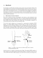
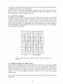


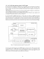
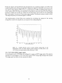
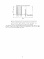

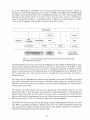


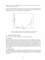


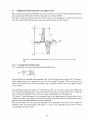

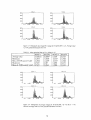
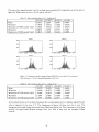


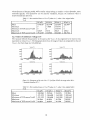
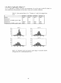
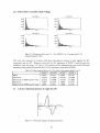
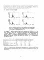

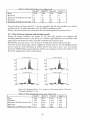
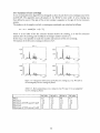

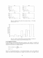
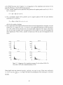

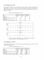
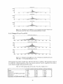
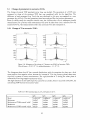
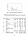
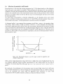

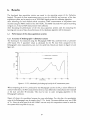
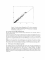


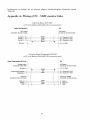

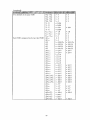


![ECG Nihon Kodhen [Mode de compatibilité]](http://vs1.manualzilla.com/store/data/006373261_1-c7a55e152165c93d2a2510c9cc5bb427-150x150.png)