Download Implementation of Data Compression Algorithm for Wireless Sensor

International Journal of Advanced Research in Electronics and Communication Engineering (IJARECE)
Volume 3, Issue 11, November 2014
Implementation of Data Compression Algorithm
for Wireless Sensor Network using K-RLE
Ranjeet S. Pisal
Assistant professor, Department of Electronics & Telecommunication
S.B. Patil College of Engineering, Indapur

Abstract— In use of Wireless Sensor Network technology for
environmental monitoring, the two main fundamental activities
of Wireless Sensor Network are data acquisition and data
transmission. However, transmitting or receiving data are
power consuming task. In order to reduce power consumption
during transmission, we introduce data compression by
processing information locally. Power saving is a critical issue in
wireless sensor networks since sensor nodes are powered by
batteries which cannot be generally changed or recharged. As
radio communication is the main cause of energy consumption,
to increase the lifetime of sensor node is generally achieved by
reducing transmissions or receptions of data, for instance
through data compression. In this article, we introduce
implementation of K-RLE compression algorithm on an
ARM7 microcontroller LPC2148 used for designing Wireless
Sensor Network.
Index Terms— Wireless sensor network (WSN), data
compression, K-RLE algorithm, embedded system, energy
efficiency.
I. INTRODUCTION
In order for wireless sensor networks to exploit signal, signal
data must be received at a multitude of sensors and must be
shared among the sensors. The vast sharing of signals among
the sensors contradicts the requirements (high energy
efficiency, low latency and high accuracy) of wireless
networked sensor. Although many techniques have been
proposed in the past (routing, scheduling, sleep modes etc.), a
new aspect is proposed here: using data compression methods
as a tool for accomplishing the optimal trade-off between data
rate, energy consumption, and accuracy in a sensor network.
Scheduling sensor states is a technique that decides which
sensor may change its state (transmit, receive, idle, Sleep),
according to the current and anticipated communications
needs. The most common technique for saving energy is the
use of sleep mode where significant parts of the sensor’s
transceiver are switched off. In most cases, the radio
transceiver on board sensor nodes is the main cause of energy
consumption hence, it is necessary to keep the transceiver in
switched off mode most of the time to reduce energy
consumption. Nevertheless, using the sleep mode reduces
data transmission or reception rate and thus communication in
the network.
The question is how to keep the same data rate sent to the base
station by reducing the number of transmission. In this paper,
Manuscript received Nov , 2014.
Ranjeet Sambhaji Pisal, Electronics & Telecommunication, S.B. Patil
College of Engineering, Indapur Pune, India.
we want to introduce In-network processing techniques,
reduces the amount of data to be transmitted. The in-network
processing technique is data compression and/or data
aggregation. Data compression is a process that reduces the
amount of data in order to reduce data transmitted, because
the size of the data is reduced. However, the limited resources
of sensor nodes like processor abilities or RAM have resulted
in the adaptation of existing compression algorithm to WSN’s
constraint. There are two types of compression algorithms are
available: lossless and lossy. Lossless compression is
algorithm that does not change the data, that is, when one
decompress it; it is identical to the original data. This makes
lossless algorithms best suited for documents, programs and
other types of data that needs to be in its original form. Lossy
algorithms do however change the data. So when one
decompresses it, there are some differences between the
decompressed data and the original data. The reason for
changing the data before compressing it, is because one can
achieve a higher compression ratio than if one had not
changed it. This is why lossy algorithms are mostly used to
compress pictures and sounds. The best known lossless
compression Algorithm for WSN is S-LZW. Nevertheless,
S-LZW which is used for WSN. The popular LZW data
compression algorithm is a dictionary-based algorithm. It
requires large use of RAM: such algorithms cannot be applied
to most sensor platform configurations due to limited RAM.
We introduce a generic data compression algorithm usable by
several sensor platforms. In this paper, we study the
adaptation of a basic compression algorithm called Run
Length Encoding (RLE). It is called as K- RLE algorithm.
The compression algorithms
A very popular lossless dictionary-based compression
algorithm is LZW which is a variant of LZ78. The best known
data compression algorithm for WSN is S-LZW which is a
version of the previous popular algorithm LZW adapted for
WSN.
1.1 LZ78
The LZ78 algorithm is a fairly simple technique. Instead of
having a window as a dictionary, as LZ77 has, it keeps the
dictionary outside the sequence so to speak. This means that
the algorithm is building the dictionary at the same time as the
encoding proceeds. When decoding, we also build the
dictionary at the same time as we decode the data stream.
Furthermore, the dictionary has to be built in the same way as
it was built in the encoding procedure. When decoding, the
algorithm is using a double, <i, s>, to access the
dictionary.The i is the index to the dictionary with the longest
match, while the s is the symbol that is after the match. Let us
go through an example to demonstrate how the technique
works. Let say that we have an alphabet A= {a, b, c, d} and we
1663
ISSN: 2278 – 909X
All Rights Reserved © 2014 IJARECE
International Journal of Advanced Research in Electronics and Communication Engineering (IJARECE)
Volume 3, Issue 11, November 2014
want to compress the sequence abbcbbaabcddbccaabaabc.
What we do first is to see if the first symbol exists in the
dictionary. In this case the first symbol is an a, so we check if
this symbol exists in the dictionary. Since the dictionary is
empty at first, we will not find it. So what we do is that we add
this symbol to the dictionary and write a double to the
compression output. In this case we write <0, a>. The next
symbol is a b, so we add this to the dictionary and write the
double <0, b>. In this step the dictionary will have the look
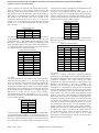
given in table I:
Table I: Dictionary
Dictionary
Index
String
Output
1
a
<0, a>
2
b
<0, b>
The next symbol in the sequence is also a b, with the index 2
in the dictionary, so what we do now is to take the next
symbol, which is a c, and combine the two symbols so we get
the string bc. This string does not exist in the dictionary so we
add it. The double that we write to the output will look like <2,
c>. Continuing in this way the dictionary will at the end have
the strings as shown in the table II below.
Table II: Final dictionary
Dictionary
Index String
Output
1
a
<0, a>
2
b
<0, b>
3
bc
<2, c>
4
bb
<2, b>
5
aa
<1, a>
6
bcd
<3, d>
7
d
<0, d>
8
bcc
<3, c>
9
aab
<5, b>
10
aabc
<9, c>
1.2 LZW
The LZW algorithm is very similar to the LZ78 algorithm.
Instead of having a double, <i, s>, the LZW is using some
tricks to remove the need for the second field in the double.
First, the dictionary contains the whole alphabet at the
beginning of encoding and decoding. Second, when building
the dictionary, the last symbol in some string will always be
the first symbol in the index below. An example will show
better how it works. Let us use the same sequence,
abbcbbaabcddbccaabaabc, and alphabet, A= {a, b, c, d}, as
in Example given below. The dictionary will at the beginning
is given in table III below.
Table III: Dictionary of LZW
Dictionary
Index
String
1
a
2
b
3
c
4
d
The first symbol in the sequence is an a. This symbol does
exist in the dictionary as index 1, so the next thing we do is to
combine the symbol a with the next symbol in the sequence, in
this case a b. We now have the string ab, which does not exist
in the dictionary, so we add it to index 5, and encode a 1 to the
output since the symbol a already exists in the dictionary. The
next step we do is to take the symbol b in the
string ab, and concatenate with the next symbol in the
sequence, b. That way we create the string bb. This string does
not exist in the dictionary so we add it, and encode a 2 to the
output, since the symbol b is in the dictionary. The appearance
of the dictionary is given in table IV below.
Table IV: Dictionary
Dictionary
Index
String
1
a
2
b
3
c
4
d
5
ab
6
bb
When we have encoded the whole sequence, we will have the
dictionary given in table V below and the output is 1 2 2 3 6 1
5 3 4 4 7 3 10 2 17.
Table V: Final Dictionary
Dictionary
Index
String
Index
String
1
a
11
abc
2
b
12
cd
3
c
13
dd
4
d
14
db
5
ab
15
bcc
6
bb
16
ca
7
17
bc
aab
8
18
cb
ba
9
19
bba
aabc
10
aa
1.3 S-LZW
S-LZW is a lossless compression algorithm purposely
developed to be embedded in sensor nodes. S-LZW splits the
uncompressed input bit stream into fixed size blocks and then
compresses separately each block. During the block
compression, for each new string, that is, a string which is not
already in the dictionary, a new entry is added to the
dictionary. For each new block, the dictionary used in the
compression is re-initialized by using the 256 codes which
represent the standard character set. Due to the poor storage
resources of sensor nodes, the size of the dictionary has to be
limited. Thus, since each new string in the input bit stream
produces a new entry in the dictionary, the dictionary might
become full. If this occurs, an appropriate strategy has to be
adopted. For instance, the dictionary can be frozen and used
to compress the remainder of the data in the block (in the
worst case, by using the code of each character), or it can be
reset and started from scratch. To take advantage of the
repetitive behavior of sensor data, a mini-cache is added to
S-LZW: the mini-cache is a hash-indexed dictionary of size
N, where N is a power of 2 that stores recently used and
created dictionary entries. Further, the repetitive behavior can
be used to pre-process the raw data so as to build
appropriately structured datasets, which can perform better
with the compression algorithm.
1664
ISSN: 2278 – 909X
All Rights Reserved © 2014 IJARECE
International Journal of Advanced Research in Electronics and Communication Engineering (IJARECE)
Volume 3, Issue 11, November 2014
1.4 Run-Length Encoding
RLE is a simple compression algorithm used to compress
sequences containing subsequent repetitions of the same
character. By compressing a particular sequence, we obtain its
code. The idea is to replace repetitions of a given character
(like aaaaa) with a counter saying how many repetitions there
are. Namely, we represent it by a triple containing a repetition
mark, the repeating character and an integer representing the
number of repetitions. For example, aaaaa can be encoded as
#a5 (where # represents the repetition mark). We need to
somehow represent the alphabet, the repetition mark, and the
counter. Let the alphabet consist of n characters represented
by integers from the set Σ = {0, 1, ..., n − 1}. The code of a
sequence of characters from Σ is also a sequence of characters
from Σ. At any moment, the repetition mark is represented by
a character from Σ, denoted by e. Initially e is 0, but it may
change during the coding. The code is interpreted as follows:
i) Any character a in the code, except the repetition
mark, represents itself
ii) If the repetition mark e occurs in the code, then the
two following characters have special meaning:
If e is followed by ek, then it represents k + 1
repetitions of e, Otherwise, if e is followed by
b0(where b ≠ e), then b will be the repetition mark
from that point on, Otherwise, if e is followed by bk
(where b ≠ e and k > 0),
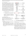
1.5 K-Run-Length Encoding
The idea behind this new algorithm is this:
Let K be a number, If a data item d or data between d+K
and d-K occur n consecutive times in the input stream, we
replace the n occurrences with the single pair nd.
We introduce a parameter K which is a precision. K is
defined as:
 δ = K/σ with σ a minimum estimate of the Allan standard
deviation.
 If K = 0, K-RLE becomes RLE. K has the same unit as the
dataset values, in this case degree.
However, the change on RLE using the K-precision
introduces data modified. Indeed, while RLE is a lossless
compression algorithm K-RLE is a lossy compression
algorithm. This algorithm is lossless at the user level
because it chooses K considering that there is no
difference between the data item d, d+K or d-K according
to the application.
Fig. I. K-RLE Compression Algorithm
Fig. I shows the graphical representation of the K-RLE
algorithm which is a variant of the RLE algorithm.
2. Experimental results
In this section, we describe the results obtained using
the previous compression algorithms on a real temperature
data sets. Certainly, data compression algorithm results
depend on the data source that is why we consider our
algorithms in real different conditions. After that, we use the
data compression ratio to estimate the performance of our
compression algorithms. It is defined as:
Compression ratio = 100 * (1- compressed size/ initial size)
However, because we cannot apply S-LZW on a sensor
platform due to a limited RAM such as one which is based on
LPC2138 for example, we have tried to increase the
compression ratio by using a variant of RLE named K-RLE.
We have used different values of K which are 0, 1, 2 and 3.
1665
ISSN: 2278 – 909X
All Rights Reserved © 2014 IJARECE
International Journal of Advanced Research in Electronics and Communication Engineering (IJARECE)
Volume 3, Issue 11, November 2014
between the original data and decompressed data. Indeed, the
feature of lossy compression is that compressing data and then
decompressing it retrieves data that may well be different
from the original data, but is close enough to be useful that is
why the precision is chosen by the user according to the
application. In comparison with S-LZW which also has a
good ratio compression, it is usable on a sensor platform with
a limited RAM.
Fig. II: Compression ratio
Fig. II shows that the as parameter ‘K’ increases, compression
ratio increases. For K=0, 1, 2 and 3 the compression ratios are
61.64%, 64.94%, 79.65% and 99.56% respectively. As we
consider value of K=0, K-RLE algorithm get converted into
RLE algorithm. These results show that the choice of K is a
very important criterion. In contrast, K-RLE can achieve
higher compression ratios at the cost of data precision when K
increases.
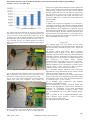
Fig. III: Transmitter node (slave node)
Fig. III shows that the transmitter node (slave node) sense
three temperatures using three sensors and when current
temperature within range then it will increase the count.
Fig. IV shows when current temperature increases and goes
outside the range then transmitter will transmit the
temperature and count to the receiver node (master node).
3. Conclusion
A K-RLE data compression algorithm on an LPC2138 is
evaluated by compressing real temperature datasets. Because
of the difficulty in using S-LZW on a sensor platform with a
limited RAM, We have implemented a algorithm inspired
from RLE named K-RLE which increases the compression
ratio compared to RLE. We have obtained compression ratio
64.94%, 79.65% and 99.56% for K=1, 2 and 3 respectively.
Hence by using K-RLE data compression algorithm we can
achieve maximum compression ratio.
REFERENCES
[1] V. Bhagya Raju, Dr K. Jaya Sankar, Dr C.D. Naidu.
Performance Evaluation of Basic Compression Technique for
Wireless Text Data. ICACSE 2013 Vol.2, No.1, Pages: 383
– 387, 2013.
[2] Eug`ene Pamba Capo-Chichi, Herv´e Guyennet,
Jean-Michel Friedt. K-RLE: A new Data Compression
Algorithm forWireless Sensor Network. Third International
Conference on Sensor Technologies and Applications, 2009.
[3] F. Marcelloni and M. Vecchio. A simple algorithm for
data compression in wireless sensor networks.
Communications Letters, IEEE, 12(6):411–413, June 2008.
[4] Croce, Silvio, Marcelloni, Francesco, Vecchio, and
Massimo. Reducing power consumption in wireless sensor
networks using a novel approach to data aggregation.
Computer Journal, 51(2):227–239, March 2008.
[5] C. M. Sadler and M. Martonosi. Data compression
algorithms for energy-constrained devices in delay tolerant
networks. In SenSys, pages 265–278, 2006.
[6] N. Kimura and S. Latifi. A survey on data compression in
wireless sensor networks. In Information Technology: Coding
and Computing, 2005. ITCC 2005. International Conference
on, volume 2, pages 8–13 Vol. 2, 2005.
[7] D. Salomon. Data Compression: The Complete
Reference. Second edition, 2004.
[8] B. Krishnamachari, D. Estrin, and S. B. Wicker. The
impact of data aggregation in wireless sensor networks. In
ICDCSW ’02: Proceedings of the 22nd International
Conference on Distributed Computing Systems, pages
575–578, Washington, DC, USA, IEEE Computer Society,
2002.
[9] I. F. Akyildiz, W. Su, Y. Sankarasubramaniam, and E.
Cayirci. Wireless sensor networks: a survey. Computer
Networks, 38(4):393–422, 2002.
[10] User manual of LPC2138 ARM7.
Fig. IV: Receiver node (master node)
We can continue to increase the K-RLE’s compression ratio
by increasing the value of K at the cost of the difference
1666
ISSN: 2278 – 909X
All Rights Reserved © 2014 IJARECE