Download Computer implementation of the CBS algorithm

Computer implementation of the
CBS algorithm
-
P. Nithiarasu*
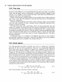
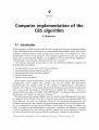
9.1 Introduction
In this chapter we shall consider some essential steps in the computer implementation
of the CBS algorithm on structured o r unstructured finite element grids. Only linear
triangular elements will be used and the notes given here are intended for a twodimensional version of the program. The sample program listing and user manual
along with several solved problems are available to down load from the publisher's
free of charge.
web site http://www.bh.com/companions/fem
The program discussed can be used to solve the following different categories of
fluid mechanics problems:
1.
2.
3.
4.
5.
Compressible viscous and inviscid flow problems
Incompressible viscous and inviscid flows
Incompressible flows with heat transfer
Porous media flows
Shallow-water problems.
With further simple modifications, many other problems such as turbulent flows,
solidification, mass transfer, free surfaces, etc. can be solved. The procedures
presented here are largely based on the computer implementation discussed in
Chapter 20, Volume 1 of this book. Many programming aspects will not be discussed
here in detail and the reader is referred back to Chapter 20, Volume 1. Here it is
assumed that the reader is familiar with FORTRAN'.' and finite element procedures
discussed in this volume as well as in Volume 1 .3
We call the present program CBSflow since it is based on the CBS algorithm discussed
in Chapter 3 of this volume. We prefer to keep the compressible and incompressible flow
codes separate to avoid any confusion. However a n experienced programmer can
incorporate both parts into a single code without much memory loss. Each program listing is accompanied by some model problems which helps the reader to validate the
codes. In addition to the model inputs to programs, a complete user manual is available
to users explaining every part of the program in detail. Any error reported by readers
will be corrected and the program will be continuously updated by the authors.
Research Fellow. Department of Civil Engineering. University of Wales. Swansea, U K
The data input module 275
The modules are constructed essentially as in Chapter 20, Volume 1 starting with
(1) the data input module with preprocessing and continuing with (2) the solution
module and (3) the output module. However, unlike the generalized program of
Chapter 20, Volume 1, the program CBSflow only contains the listing for solving
transient Navier-Stokes (or Euler-Stokes) equations iteratively. Here there are
many possibilities such as fully explicit forms, semi-implicit forms, quasi-implicit
forms and fully implicit forms as discussed in Chapter 3 of this volume. We concentrate mainly on the first two forms which require small memory and simple solution
procedures compared to other forms.
In both the compressible and incompressible flow codes, only non-dimensional
equations are used. The reader is referred to the appropriate chapters of this
volume (Chapters 3 , 4 and 5 ) for different non-dimensional parameters.
In Sec. 9.2 we shall describe the essential features of data input to the program.
Here either structured or unstructured meshes can be used to divide the problem
domain into finite elements. Section 9.3 explains how the steps of the CBS algorithm
are implemented. In that section, we briefly remark on the options available for shock
capturing, various methods of time stepping and different procedures for equation
solving. In Sec. 9.4, the output generated by the program and postprocessing
procedures are considered. In the last section (Sec. 9.5) we shall consider the
possibility of further extension of CBSflow to other problems such as mass transfer,
turbulent flow, etc.
9.2 The data input module
This part of the program is the starting point of the calculation where the input data
for the solution module are prepared. Here an appropriate input file is opened and the
data are read from it. Unlike in Chapter 20, Volume 1, we have no mesh generator
coupled with CBSflow. However an advancing front unstructured mesh generator
and some structured mesh generators are provided separately. By suitable coupling,
the reader can implement various adaptive procedures as discussed in Chapters 4 and
5. Either structured or unstructured mesh data can be given as input to the program.
The general program structure and many more details can be found in Chapter 20,
Volume 1.
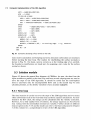
9.2.1 Mesh data - nodal coordinates and connectivity
Once the nodal coordinates and connectivity of a finite element mesh are available
from a mesh generator, they are allotted to appropriate arrays (for a detailed description on the mesh, numbering etc., see Chapter 20, Volume I). Essentially the same
arrays as described in Chapter 20, Volume 1 are used here. The coordinates are
allotted to X ( i , j ) with i defining the appropriate Cartesian coordinates x l ( i = I )
and x 2 ( i = 2) and j defining the global node number. Similarly the connectivity is
allotted to an array I X ( k , / ) .Here k is the local node number and 1 is the global
element number. It should be noted that the material code normally used in heat
conduction and stress analysis is not necessary.
276
Computer implementation of the CBS algorithm
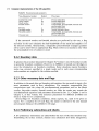
Table 9.1 Non-dimensional parameters
Non-dimensional number
Symbol
Flow types
Conductivity ratio
Darcy number
Mach number
Prandtl number
k"
Da
M
Pr
Porosity
Rayleigh number
Reynolds number
E
Viscosity ratio
v
Porous media flows
Porous media flows
Compressible flows
Compressible, incompressible, thermal and
porous media flows
Porous media flows
Natural convective flows
Compressible, incompressible, thermal and
porous media flows
Porous media flows
Ra
Re
If the structured meshes and banded solution are preferred by the user, a flag
activated by the user calculates the half-bandwidth of the mesh and supplies it to
the solution module. Alternatively, a diagonally preconditioned conjugate gradient
solver can be used with an appropriate flag. These solvers are necessary only when
the semi-implicit form of solution is used.
9.2.2 Boundary data
In general, the procedure discussed in Chapter 20, Volume 1 uses the boundary nodes
to prescribe boundary conditions. However, in CBSflow we mostly use the edges to
store the information on boundary conditions. Some situations require boundary
nodes (e.g. pressure specified in a single node) and in such cases corresponding
node numbers are supplied to the solution module.
9.2.3 Other necessary data and flags
In addition to the mesh data and boundary information, the user needs to input a few
more parameters used in flow calculations. For example, compressible flow
computations need the values of non-dimensional parameters such as the Mach
number, Reynolds number, Prandtl number, etc. Here the reader may consult the
non-dimensional equations and parameters discussed in Sec. 3.1, Chapter 3, and in
Chapter 5, of this volume. The necessary parameters for different problems are
listed in Table 9.1 for completeness.
Several flags for boundary conditions, shock capture, etc. need to be given as
inputs. For a complete list of such flags, the reader is referred to the user manual
and program listing at the publisher's web page.
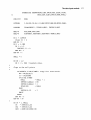
9.2.4 Preliminarv subroutines and checks
A few preliminary subroutines are called before the start of the time iteration loop.
Establishing the surface normals, element area calculation (for direct integration),
The data input module 277
SUBROUTINE GETNRW(MXPOI,MBC,NPOIN,NBS,ISIDE,IFLAG,
COSX,COSY,ALEN,IWPOIN,WNOR,NWALL)
€!
IMPLICIT
NONE
INTEGER
I,IB,IB2,IN,IW,J,JJ,MBC,MXPOI,NBS,NN,NPOIN,NWALL
REAL*8
REAL*8
ACH,ANOR,ANXl,ANYl
ALEN(MBC) ,COSX(MBC) ,COSY(MBC) WNOR(2,MBC)
DO I = 1,NPOIN
IFLAG (I) = 0
END DO ! I
DO I = 1, NBS
DO J = 1,3
IWPOIN(J,I)
END DO ! J
END DO ! I
NWALL
=
=
0
0
DO IN = 1,2
DO I = 1, NBS
! boundary s i d e s
C
c
flags on t h e wall p o i n t s
IF(ISIDE(4,I).EQ.2)THEN
NN = ISIDE(IN,I)
JJ = IFLAG(")
IF(JJ.EQ.0)THEN
=
NWALL
IWPOIN(1,NWALL) =
IWPOIN(2,NWALL) =
IFLAG(")
=
ELSE
=
IWPOIN(3,JJ)
ENDIF
ENDIF
END DO ! I
END DO ! IN
C
DO IW = 1, NWALL
IB = IWPOIN(2,IW)
IB2 = IWPOIN(3,IW)
ANXl = ALEN(IB)*COSX(IB)
! flag 2 f o r s o l i d walls.
NWALL + 1
NN
I
NWALL
I
278
Computer implementation of the CBS algorithm
ANYl = ALEN(IB)*COSY(IB)
ACH = O.ODO0
IF(IB2.NE.O)THEN
ANXl = ANXl + ALEN(IB2)*COSX(IB2)
ANYl = ANYl + ALEN(IB2)*COSY(IB2)
ACH = COSX(IB)*COSX(IB2) + COSY(IB)*COSY(IB2)
ENDIF
ANOR
= DSQRT(ANXl*ANXl + ANYl*ANYl)
ANX 1
= ANXl/ANOR
ANY 1
= ANYl/ANOR
WNOR(1,IW)
= ANXl
WNOR(2,IW)
= ANYl
IF(ACH.LT.-0.2) THEN
WNOR(1,IW) = O.ODO0
WNOR(2,IW) = O.ODO0
WRITE(*,*)IWPOIN(l,IW),’
is trailing edge’ ! e.g. aerofoil
ENDIF
END DO ! IW
END
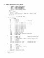
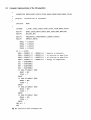
Fig. 9.1 Subroutine calculating surface normals on the walls
mass matrix calculation and lumping and some allocation subroutines are necessary
before starting the time loop. The routine for establishing the surface normals is
shown in Fig. 9.1. On sharp, narrow corners as at the trailing edge of an aerofoil,
the boundary contributions are made zero by assigning a zero value for the surface
normal as shown.
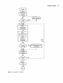
9.3 Solution module
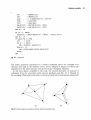
Figure 9.2 shows the general flow diagram of CBSflow. As seen, the data from the
input module are passed to the time loop and here several subprograms are used to
solve the steps of the CBS algorithm. It should be noted that the semi-implicit
form is used here only for incompressible flows and at the second step we only
calculate pressure, as the density variation is here assumed negligible.
9.3.1 Time loop
The time iteration is carried out over the steps of the CBS algorithm and over many
other subroutines such as the local time step and shock capture calculations. As mentioned in the flow chart, the energy can be calculated after the velocity correction.
However, for a fully explicit form of solution, the energy equation can be solved in
step 1 along with the intermediate momentum variable. Further details on different
steps are given in Sec. 9.3.4 and the reader can refer to the theory discussed in Chapter
3 of this volume for a comprehensive review of the CBS algorithm.
Solution module 279
Fig. 9.2 Flow diagram for CBSflow.
280 Computer implementation of the CBS algorithm
9.3.2 Time step
-In general, three different ways of establishing the time steps are possible. In problems
where only the steady state is of importance, so-called ‘local time stepping’ is used
(see Sec. 3.3.4, Chapter 3). Here a local time step at each and every nodal points is
calculated and used in the computation.
When we seek accurate transient solution of any problem, the so-called ‘minimum
step’ value is used. Here the minimum of all local time step values is calculated and
used in the computation.
Another and less frequently used option is that of giving a ‘fixed’ user-prescribed
time step value. Selection of such a quantity needs considerable experience from
solving several flow problems.
The times loop starts with a subroutine where the above-mentioned time step
options are available. In general the local time steps are calculated at every iteration
for the initial few time steps and then they are calculated only after a certain number
of iterations as prescribed by the user. If the last option of the user-specified fixed time
step is used, the local time steps are not calculated. Figure 9.3 shows the subroutine
used for calculating the local time steps for inviscid compressible flows with linear
triangular elements.
As indicated in Sec. 4.3.3, Chapter 4, two different time steps are often useful in
getting better stabilization procedure^.^ Such internal (DELTI) and external (DELTP)
time stepping options are available in the routine of Fig. 9.3.
9.3.3 Shock capture
The CBS algorithm introduces naturally some terms to stabilize the oscillations
generated by the convective acceleration. However, for compressible high-speed
flows, these terms are not sufficient to suppress the oscillations in the vicinity of
shocks and some additional artificial viscosity terms need to be added (see Sec. 6.5,
Chapter 6). We have given two different forms of artificial viscosities based on the
second derivative of pressure in the program. Another possibility is to use anisotropic
shock capturing based on the residual of individual equations solved. However we
have not used the second alternative in the program as the second derivative based
procedures give quite satisfactory results for all high-speed flow problems.
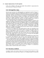
In the first method implemented, we need to calculate a pressure switch (see Eq.
(6.16), Chapter 6) from the nodal pressure values. Figure 9.4 gives a typical example
of triangular elements inside and on the boundaries. For inside nodes (Fig. 9.4(a)) we
calculate the nodal switch as
and for the boundary node (Fig. 9.4(b)) we calculate
Solution module 281
SUBROUTINE TIMSTP(MXPOI,MXELE,NELEM,NPOIN,IALOT, IX, SFACT,
DTFIX,UNKNO,DELTP,DELTI,SONIC,PRES,GAMMA,
&
GEOME, X, NMAX,MAXCON,MODEL, NODEL)
&
c calculates the critical local time steps at nodes.
c calculates internal and external time steps.
IMPLICIT NONE
IMPLICIT MPOI
PARAMETER(MPOI=9000)
INTEGER
INTEGER
I,IALOT,IE,IP,IPl,IP2,IP3,MODEL,M~~~E,MX~~~
NELEM,NODEL,NPOIN
INTEGER
IX(MODEL,MXELE) ,MAXCON(20 ,MIXPOI),NMAX(MXPOI)
REAL*8
REAL*8
ALEN,ANX,ANY,CMAX, DTFIX, DTP, GAMMA, SFACT,TSTI
TSTP,U,Ul,U2,U3,V,Vl,V2,V3,VNl,VN2,VN3,VELN,VSUM
REAL*8
REAL*8
REAL*8
REAL*8 PRS(MPO1) ,RHO(MPOI) ,VMAG(MPOI) ,VNORM(MPOI) ! local arrays
IF(IALOT.EQ.-1)THEN
CALL TIMFIL(MXPOI,DELTP,NPOIN,DTFIX)
CALL TIMFIL(MXPOI,DELTI,NPOIN,DTFIX)
RETURN
ENDIF
c smoothing the variables
C
DO I = 1, NPOIN
VNORM(1)
= O.OOD+OO
= O.OOD+OO
RHO(1)
= O.OOD+OO
PRS(1)
= UNKN0(2,I)/UNKNO(l,I)
U
= UNKN0(3,I)/UNKNO(l,I)
V
= DSQRT(U**2+V**2)
VMAG(1)
DO IP = l,NMAX(I)
= MAXCON(IP,I)
IP1
VNORM(1) = VNORM(1) + VMAG(IP1)
= PRS(1) + PRES(IP1)
PRS(1)
RHO(I)
= RHO(I) + UNKNO(~,IP~)
END DO ! IP
Fig. 9.3 Subroutine for time step calculation.
282
Computer implementation of the CBS algorithm
VNORM(1) = VNORM(I)/FLOAT(NMAX(I))
= PRS(I)/FLOAT(NMAX(I))
PRS(1)
= RHO(I)/FLOAT(NMAX(I))
RHO(1)
SONIC(1) = DSQRT(GAMMA*PRS(I)/RHO(I))
END DO ! I
DO IP = 1,NPOIN
DELTP(1P) = 1.0d06
SONIC(1P) = DSQRT(GAMMA*PRES(IP)/UNKNO(l,IP))
END DO ! IP
! speed of sound
C
c loop for calculation of local time steps
C
DO IE = 1, NELEM
= IX(1,IE)
IP1
IP2
= IX(2,IE)
!
IP3
= IX(3,IE)
= UNKN0(2,IPl)/UNKNO(l,IPl)
!
u1
v1
= UNKN0(3,IPl)/UNKNO(l,IPl)
!
u2
= UNKN0(2,IP2)/UNKNO(l,IP2)
v2
= UNKN0(3,IP2)/UNKNO(l,IP2)
u3
= UNKN0(2,IP3)/UNKNO(l,IP3)
v3
= UNKN0(3,IP3)/UNKNO(l,IP3)
VN 1
= DSQRT(U1**2 + U1**2)
VN2
= DSQRT(U2**2 + U2**2)
= DSQRT(U3**2 + U3**2)
VN3
= MAX(VN1, VN2, VN3)
VELN
CMAX
= MAX(SONIC(IPl),
SONIC(IP2),
= VELN + CMAX
VSUM
connectivity
ul velocity
u2 velocity
SONIC(IP3))
C
ANX
ANY
ALEN
TSTP
TSTI
DELTP(IP1)
DELTI(IP1)
=
ANX
=
ANY
ALEN
TSTP
TSTI
DELTP(IP2)
DELTI(IP1)
=
=
=
=
=
=
=
GEOME(1,IE)
GEOME(4, IE)
l.O/DSQRT(ANX**2 + ANY**2)
ALEN/VSUM
ALEN/VELN
MIN(DELTP(IPl), TSTP)
MIN(DELTI(IPl), TSTI)
C
Fig. 9.3 Continued.
=
=
=
=
=
GEOME(2, IE)
GEOME(5, IE)
1.O/DSQRT(ANX**2 + ANY**2)
ALEN/VSUM
ALEN/VELN
MIN(DELTP(IP2), TSTP)
MIN(DELTI(IPl), TSTI)
! shape function derivatives
! element length at node 1
! external time step
! internal time step
Solution module 283
C
ANX
ANY
ALEN
TSTP
TSTI
DELTP(IP3)
DELTI(IP1)
END DO ! IE
=
=
=
=
=
=
=
GEOME(3,IE)
GEOME(6, IE)
l.O/DSQRT(ANX**2 + ANY**2)
ALEN/VSUM
ALEN/VELN
MIN(DELTP(IP3), TSTP)
MIN(DELTI(IPl), TSTI)
DO IP = 1, NPOIN
DELTP(1P) = SFACT*DELTP(IP) ! SFACT - s a f e t y f a c t o r
END DO ! IP
IF(IALOT.EQ.0) THEN
DTP
= 1.0d+06
DO IP = 1,NPOIN
DTP = MIN(DTP, DELTP(1P))
END DO ! IP
CALL TIMFIL(MXPOI,DELTP,NPOIN,DTP)
ENDIF
END
Fig. 9.3 Continued.
The nodal quantities calculated in a manner explained above are averaged over
elements and used in the relations of Eq. (6.17), Chapter 6. Figure 9.5 shows the
calculation of the nodal pressure switches for linear triangular elements.
In the next option available in the code, the second derivative of pressure is
calculated from the smoothed nodal pressure gradients (see Sec. 4.5.1, Chapter 4)
by averaging. Other approximations to the second derivative of pressure are described
Fig. 9.4 Typical element patches (a) interior node (b) boundary node.
284 Computer implementation of the CBS algorithm
in Sec. 4.5.1, Chapter 4. The user can employ those methods to approximate the
second derivative of pressure if desired.
9.3.4 CBS algorithm. Steps
Various steps involved in the CBS algorithm are described in detail in Chapter 3.
There are three essential steps in the CBS algorithm (Fig. 9.2). First, an intermediate
momentum variable is calculated and in the second step the density/pressure field is
determined. The third step involves the introduction of density/pressure fields to
obtain the correct momentum variables. In problems where the energy and other
variables are coupled, calculation of energy is necessary in addition to the above
three steps. In fully explicit form, however, the energy equation can be solved in
the first step itself along with the intermediate momentum calculations.
In the subroutine s t e p 1 we calculate the temperature-dependent viscosity at the
beginning according to Sutherland’s relation (see Chapter 6). The averaged viscosity
values over each element are used in the diffusion terms of the momentum equation
and dissipation terms of the energy equation. The diffusion, convective and stabilization terms are integrated over elements and assembled appropriately to the RHS
vector. The integration is carried out either directly or numerically. Finally the
RHS vector is divided by the lumped mass matrices and the values of intermediate
momentum variables are established.
In step two, in explicit form, the density/pressure values are calculated by the
Eq. (3.53) (or Eq. (3.54)). The subroutine s t e p 2 is used for this purpose. Here the
option of using different values of 01 and 02 is available. In explicit form 02 is
identically equal to zero and O1 varies between 0.5 and 1.0. For compressible flow
computations, the semi-implicit form with 4 greater than zero has little advantage
over the fully explicit form. For this reason we have not given the semi-implicit
form for compressible flow problems in the program.
For incompressible flow problems, in general the semi-implicit form is used. In this
&, as before, varies between 0.5 and 1 and e2 is also in the same range. Now it is
essential to solve the pressure equation in s t e p 2 of the algorithm. Here in general
we use a conjugate gradient solver as the coefficient matrix is not necessarily banded.
The third step is the one where the intermediate momentum variables are corrected
to get the real values of the intermediate momentum. In all three steps, mass matrices
are lumped if the fully explicit form of the algorithm is used. As mentioned in earlier
chapters, this is the best way to accelerate the steady-state solution along with local
time stepping. However, in problems where transient solutions are of importance,
either a mass matrix correction as given in Sec. 2.6.3, Chapter 2 or simultaneous
solution using a consistent mass matrix is necessary.
9.3.5 Boundary conditions
As explained before, the boundary edges are stored along with the elements to which
they belong. Also in the same array i s i d e ( i , j > the flags necessary to inform the
Solution module
&
SUBROUTINE SWITCH(MXPO1, MXELE, MBC, NPOIN, NELEM, NBS, PRES,
CSHOCK,PSWTH,IX,DELUN,ISIDE,MODEL,ITYPE)
C
c this subroutine calculates the pressure switch at each node
c maximum value 1 and minimum value 0
C
IMPLICIT
NONE
INTEGER
INTEGER
IB,IELEM,IP,IP1,IP2,IP3,ITYPE,MBC,MODEL
MXELE,MXPOI,NBS,NELEM, NPOIN
INTEGER
ISIDE(4 ,MBC),IX(MODEL,MXELE)
REAL*8
REAL*8
CSHOCK, PADD, P11, P22, P33,PSl,PS2,PS3
XPS ,XPD
REAL*8
DELUN (MXPOI) ,PRES(MXPOI) ,PSWTH(MXP0.I)
C
DO IELEM = 1,NELEM
IP1
= IX(1,IELEM)
IP2
= IX(2,IELEM)
IP3
= IX(3,IELEM)
PS1
= PRES(IP1)
PS2
= PRES(IP2)
PS3
= PRES(IP3)
= PSl+PS2+PS3
PADD
P11
= (3.0dOO*PSl - PADD)
P22
= (3.0dOO*PS2 - PADD)
P33
= (3.0dOO*PS3 - PADD)
PSWTH(IP1) = PSWTH(IP1) + P11
PSWTH(IP2) = PSWTH(IP2) + P22
PSWTH(IP3) = PSWTH(IP3) + P33
DELUN(IP1) = DELUN(IP1) + DABS(PS1 - PS2) + DABS(PS1 - PS3)
DELUN(IP2) = DELUN(IP2) + DABS(PS1 - PS2) + DABS(PS2 - PS3)
DELUN(IP3) = DELW(IP3) + DABS(PS3 - PS2) + DABS(PS1 - PS3)
END DO ! IELEM
DO IB = 1,NBS
IP1
= ISIDE(1, IB)
= ISIDE(2,IB)
IP2
PS1
= PRES(IP1)
PS2
= PRES(IP2)
= PS1 + PS2
XPS
XPD
= PS1 - PS2
PSWTH(IP1) = PSWTH(IP1) + XPD
PSWTH(IP2) = PSWTH(IP2) - XPD
DELUN(IP1) = DELUN(IP1) + DABS(XPD)
DELUN(IP2) = DELUN(IP2) + DABS(XPD)
285
286 Computer implementation of the CBS algorithm
END DO ! IB
DO IP = 1,NPOIN
IF(DELUN(IP).LT.O.l*PRES(IP))DELUN(IP)
= PRES(1P)
END DO ! IP
DO IP = 1,NPOIN
PSWTH(1P) = CSHOCK*DABS(PSWTH(IP))/DELUN(IP)
END DO ! IP
END
Fig. 9.5 Calculation of nodal pressure switches for shock capturing
solution module which type of boundary conditions are stored. In this array i = 1,2
correspond to the node numbers of any boundary side of an element, i = 3 indicates
the element to which the particular edge belongs and i = 4 is the flag which
indicates the type of boundary condition (a complete list is given in the user manual
available at the publisher’s web page). H e r e j is the boundary edge number. A typical
routine for prescribing the symmetry conditions is shown in Fig. 9.6.
9.3.6 Solution of simultaneous equations - semi-implicit form
The simultaneous equations need to be solved for the semi-implicit form of the CBS
algorithm. Two types of solvers are provided. The first one is a banded solver which is
effectivewhen structured meshes are used. For this the half-bandwidth is necessary in
order to proceed further. The second solver is a diagonal preconditioned conjugate
gradient solver. The latter can be used to solve both structured and unstructured
meshes. The details of procedures for solving simultaneous equations can be found
in Chapter 20 of Volume 1.
9.3.7 Different forms of energy equation
In compressible flow computations only the fully conservative form of all equations
ensures correct position of shocks. Thus in the compressible flow code, the energy
equation is solved in its conservative form with the variable being the energy.
However for incompressible flow computations, the energy equation can be written
in terms of the temperature variable and the dissipation terms can be neglected. In
general for compressible flows, Eq. (3.61) is used, and Eq. (4.6) is used for incompressible flow problems.
9.3.8 Thermal and porous media flows
As mentioned earlier the heat transfer and porous medium flows are also included
in the incompressible flow code. Using the heat transfer part of the code, the user
can solve forced, natural and mixed convection problems. Appropriate flags and
Solution module 287
tL
SUBROUTINE SYMMET(MXPO1, MBC, NPOIN, NBS, UNKNO,ISIDE,RHOINF,
UINF,VINF, COSX,COSY)
C
c symmetric boundary conditions forced. one component of velocity
c forced to zero
C
IMPLICIT
NONE
INTEGER
I,IP,J,MBC,MXPOI,NBS,NPOIN
INTEGER
ISIDE (4,MBC)
REAL*8
ANX,ANY,RHOINF,UINF,US,VINF
REAL*8
COSX(MBC), COSY(MBC), UNKNO(4,MXPOI)
C
DO I = 1, NBS
IF(ISIDE(4,I).EQ.4)THEN ! symmetry flag 4
ANX
= COSX(1)
= COSY(1)
ANY
DO J = 1,2
IP
= ISIDE(J,I)
us
= -UNKN0(2,IP)*ANY + UNKNO(S,IP)*ANX
UNKNO(2,IP) = - US*ANY
UNKNO(3,IP) =
US*ANX
END DO ! J
ENDIF
END DO ! I
END
Fig. 9.6 Subroutine to impose symmetry conditions.
non-dimensional parameters need to be given as input. For the detailed discussion on
these flows, the reader is referred to Chapter 5 of this volume.
9.3.9 Convergence
.
~
-----”--
-
~
_^--->
The residuals (difference between the current and previous time step values of
parameters) of all equations are checked at every few user-prescribed number of iterations. If the required convergence (steady state) is achieved, the program stops
automatically. The aimed residual value is prescribed by the user. The program
calculates the maximum residual of each variable over the domain. The user can
use them to fix the required accuracy. We give the routine used for this purpose in
Fig. 9.7.
~
288 Computer implementation of the
CBS algorithm
C
SUBROUTINE RESID(MXPOI,NPOIN,ITIME,UNKNO,UNPRE,PRES,PRESN,IFLOW~
C
c
purpose : calculations of residuals.
C
IMPLICIT
NONE
INTEGER
I,ICONl,ICON2,ICON3,ICON4,IFLOW,ITIME,MXPOI,NPOIN
REAL*8
REAL*8
EMAXl,EMAX2,EMAX3,EMAX4,ERRl,ERR2,ERR3,ERR4,ERl
REAL*8
REAL*8
PRES(MXPOI) ,PRESN(MXPOI) ,UNKNO(4,MXPOI)
UNPRE(4,MXPOI)
C
EMAXl
EMAX2
EMAX3
EMAX4
ER2,ER3,ER4
= 0.000d00
= 0.000d00
= 0.000d00
= 0.000d00
DO I = 1,NPOIN
ERR1 = UNKNO(1,I)
ERR2 = UNKNO(2,I)
ERR3 = UNKNO(3,I)
ERR4 = UNKNO(4,I)
ER1 = DABS(ERR1)
ER2 = DABS(ERR2)
ER3 = DABS(ERR3)
ER4 = DABS(ERR4)
IF (ERl.GT.EMAX1)
EMAXl = ER1
ICON1 = I
ENDIF
IF (ER2.GT.EMAX2)
EMAX2 = ER2
ICON2 = I
ENDIF
IF (ER3.GT.EMAX3)
EMAX3 = ER3
ICON3 = I
ENDIF
IF (ER4.GT.EMAX4)
EMAX4 = ER4
ICON4 = I
ENDIF
END DO ! I
END
- UNPRE(1,I)
! density or pressure
- UNPRE(2,I)
! u l velocity or mass f l u x
! u2 velocity or mass f l u x
! energy or temperature
- UNPRE(3,I)
- UNPRE(4,I)
THEN
THEN
THEN
THEN
Fig. 9.7 Subroutine to check convergence rate.
References 289
9.4 Output module
If the imposed convergence criteria are satisfied then the output is written into a
separate file. The user can modify the output according to the requirements of postprocessor employed. Here we recommend the education software developed by
CIMNE (GiD) for post and preprocessing of data.5 The facilities in GiD include
two- and three-dimensional mesh generation and visualization.
9.4.1 Stream function calculation
The stream function value is calculated from the following equation:
a2+
@.J,
-+-=---
ax:
ax;
av
8x2 ax,
au
(9.3)
This equation is derived from the definition of stream function in terms of the velocity
components. We again use the finite element method to solve the above equation.
9.5 Possible extensions to CBSflow
As mentioned earlier, there are several possibilities for extending this code. A simple
subroutine similar to the temperature equation can be incorporated to solve mass
transport. Here another variable ‘concentration’ needs to be solved.6
Another subject which can be incorporated and studied is that of a ‘free surface’
given in Chapter 5 of this volume. Here another equation needs to be solved for
the surface waves.’
The phase change problems need appropriate changes in the energy equation.8-’2
The liquid, solid and mushy regions can be accounted for in the equations by simple
modifications. The latent heat also needs to be included in phase change problems.
The turbulent flow requires solution of another set or sets of equations similar to
the momentum or energy equations as explained in Chapter 5. For the 6-E model
the reader is referred to reference 13.
The program CBSflow is an educational code which can be modified to suit the
needs of the user. For instance, the modification of this program to incorporate a
‘command language’ could make the code very efficient and compact.
References
I. Swith and D.V. Griffiths. Programming the Finite Element Method, Third Edition, Wiley,
Chichester, 1998.
D.R. Will&.Advanced Scientific Fortran, Wiley, Chichester, 1995.
O.C. Zienkiewicz and R.L. Taylor. The Finite Element Method, Vol. I, The Basics, 5th
Edition, Arnold, London, 2000.
P. Nithiarasu and O.C. Zienkiewicz. On stabilization of the CBS algorithm. Internal and
external time steps. Int. J. Num. Meth. Eng., 48, 875-80, 2000.
290 Computer implementation of the CBS algorithm
5. GiD. International Center for Numerical Methods in Engineering, Universidad PolitCcnica
de Catalufia, 08034, Barcelona, Spain.
6. P.Nithiarasu, K.N. Seetharamu and T. Sundararajan. Double-diffusive natural convection
in an enclosure filled with fluid saturated porous medium - a generalised non-Darcy
approach. Numerical Heat Transfer, Part A , Applications, 30, 413-26, 1996.
7. I.R. Idelsohn, E. Oiiate and C. Sacco. Finite element solution of free surface ship wave
problems. Int. J . Num. Meth. Eng., 45, 503-28, 1999.
8. K. Morgan. A numerical analysis of freezing and melting with convection. Comp. Meth.
Appl. Mech. Eng., 28, 275-84, 1981.
9. A S . Usmani, R.W. Lewis and K.N. Seetharamu. Finite element modelling of natural
convection controlled change of phase. Int. J . Num. Meth. Fluids, 14, 1019-36, 1992.
10. S.K. Sinha, T. Sundararajan and V.K. Garg. A variable property analysis of alloy solidification using the anisotropic porous medium approach. Int. J . Heat Mass Transfer, 35,
2865-77, 1992.
11. R.W. Lewis, K. Morgan, H.R. Thomas and K.N. Seetharamu. The Finite Element Method
for Heat Transjer Analysis, Wiley, Chichester, 1996.
12. P. Nithiarasu. An adaptive finite element procedure for solidification problems. Heat and
Muss Transfer (to appear, 2000).
13. O.C. Zienkiewicz, B.V.K.S. Sai, K. Morgan and R. Codina. Split characteristic based semiimplicit algorithm for laminar/turbulent incompressible flows. Int. J. Num. Meth. Fluids,
23, 1-23, 1996.