No category

Download Fast Marching Methods - Parallel Implementation and Analysis

100

101

102

103

104

105

106

107

108

109

110

111

112

113

114

115

116

117

118

119

120

121

122

123

124

125

126

127

128

129

130

Transcript

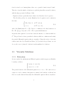
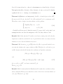
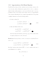
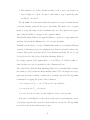
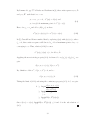
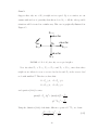
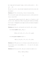
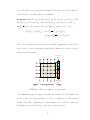
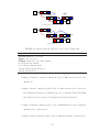
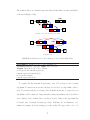
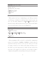
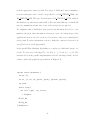
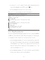
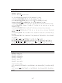
In Figure 1.7 we present the stencil structure for Rouy-Tourin algorithm and the
algorithm is presented in Algorithm 1.
Ti,j+1
Ti-1,j
R
Ti+1,j
Ti,j-1
FIGURE 1.7. Grid points for Rouy-Tourin algorithm
Algorithm 1 The Rouy-Tourin algorithm
Consider S > diam(Ω).
Initialization:
Ti,j = 0 on ∂Ω
Ti,j = S, otherwise
Iteration:
repeat
for i = 0 to n do
for j = 0 to n do
compute R solution of local Eikonal equation at Xi,j
end
end
T˜i,j = min(Ti,j , R)
T = T̃
until kT − T̃ k ≤ ε ;
For any node (i, j) in the domain we should solve the equation:
2
−x
+x
[ max max(Di,j
T, 0), − min(Di,j
T, 0)
+
2
−y
+y
max max(Di,j
T, 0), − min(Di,j
T, 0) ]1/2 =
1
,
Fi,j
(1.24)
in order to compute its Ti,j .
Let us consider the case presented in the previous section, in Figure 1.5(a), where
the third quadrant is the upwind side of our domain and show how the Rouy-Tourin
algorithm satisfies the upwind-ing. All the other possible situations can be reduced
24

Related documents