Download Statecruncher User Manual

STATECRUNCHER User Manual
Graham G. Thomason
Report Relating to the Thesis “The Design
and Construction of a State Machine
System that Handles Nondeterminism”
Department of Computing
School of Electronics and Physical Sciences
University of Surrey
Guildford, Surrey GU2 7XH, UK
July 2004
© Graham G. Thomason 2003-2004
Summary
This document is a user manual and training course for users of STATECRUNCHER.
STATECRUNCHER is a state transition language in which a dynamic model of a system (i.e. a
statechart) can be written and exercised. Given a dynamic model of a system,
STATECRUNCHER provides an oracle to state based tests. It specialises in its handling of
nondeterminism. It has been integrated by Philips Research India - Bangalore into a tool chain
to provide automated generation and execution of tests. This report assumes a basic
knowledge of UML dynamic modelling, and shows how to implement them in
STATECRUNCHER, describing both syntax and semantics.
ii
© Graham G. Thomason 2003-2004
Contents
1.
Introduction ...................................................................................................................... 1
1.1 What STATECRUNCHER is and does ...................................................................... 1
1.2 STATECRUNCHER and Prolog ............................................................................... 3
1.3 Notation ..................................................................................................................... 4
1.4 Related documentation by the present author ............................................................. 4
2.
Installation ........................................................................................................................ 5
2.1 Hardware requirements .............................................................................................. 5
2.2 Installation overview .................................................................................................. 5
2.3 To install STATECRUNCHER source from the zip file ............................................ 8
2.4 Downloading and installing SWI-Prolog.................................................................... 8
2.5 To compile and run STATECRUNCHER under SWI Prolog .................................... 9
2.6 To compile and run STATECRUNCHER under WinProlog...................................... 9
2.7 To run the STATECRUNCHER MS-DOS executable ............................................ 10
3.
Getting started ................................................................................................................ 11
4.
Guide to operation .......................................................................................................... 16
4.1 Variables, and parameterised and conditional transitions ......................................... 17
4.2 Nested cluster and history ........................................................................................ 21
4.3 Sets ........................................................................................................................... 24
4.4 Fired events .............................................................................................................. 28
4.5 Client-server composition and PCOs ....................................................................... 31
4.6 Assignments on transitions and inexact variable scoping ......................................... 34
4.7 Orbits, self-transitions, upon-enter and upon-exit actions ........................................ 38
4.8 Meta-events .............................................................................................................. 43
4.9 Conditional actions and the in() function ................................................................. 46
4.10 Strings and string functions ...................................................................................... 51
4.11 Traces ....................................................................................................................... 56
4.12 Inexact state scoping ................................................................................................ 59
4.13 Introduction to nondeterminism ............................................................................... 63
4.14 Fork nondeterminism ............................................................................................... 64
4.15 Fork nondeterminism differentiated by history and trace ......................................... 68
4.16 Scoped events illustrated by fork nondeterminism ................................................... 71
4.17 Race nondeterminism ............................................................................................... 75
4.18 Set-transit nondeterminism....................................................................................... 79
4.19 Set-action nondeterminism ....................................................................................... 83
4.20 Set meta-event nondeterminism ............................................................................... 88
4.21 Fired event and multiple nondeterminism ................................................................ 95
4.22 Transition prioritisation ............................................................................................ 98
4.23 Limited race nondeterminism ................................................................................. 104
4.24 Limited set nondeterminism ................................................................................... 108
4.25 Independence of race and set-transit control .......................................................... 112
© Graham G. Thomason 2003-2004
iii
4.26 Pruning on the basis of traces ................................................................................. 113
4.27 Arrays .................................................................................................................... 116
4.28 What else is there to STATECRUNCHER? ........................................................... 119
5.
Modelname mode ......................................................................................................... 120
5.1 To prepare your file and an index to it ................................................................... 120
5.2 Using modelname mode ......................................................................................... 121
6.
The STATECRUNCHER Release 1.02 loop ................................................................ 122
6.1 To prepare a model................................................................................................. 122
6.2 To compile and validate your file ........................................................................... 122
6.3 Exercising models .................................................................................................. 123
7.
The socket version of STATECRUNCHER ................................................................. 124
8.
Reference for STATECRUNCHER syntax .................................................................. 125
8.1 Declarations and an overview of state statements .................................................. 125
8.2 Transitions.............................................................................................................. 127
8.3 Arithmetic operators............................................................................................... 131
8.4 Scoping operators ................................................................................................... 132
8.5 The split operator ................................................................................................... 133
8.6 Functions ................................................................................................................ 134
9.
Reference for STATECRUNCHER commands............................................................ 135
10.
Glossary and abbreviations ....................................................................................... 140
11.
References ................................................................................................................ 144
iv
© Graham G. Thomason 2003-2004
1. Introduction
This document is a user manual for STATECRUNCHER . It covers the syntax and explains the
semantics, mainly by example. Both the STATECRUNCHER modelling language and the main
user commands that can be sent to it are treated.
It does not cover advanced commands that would probably only be given under program
control (by a primer), except in a reference section, nor at all the art of producing good
models from a software specification, nor does it cover software component composition
issues, except for a basic client-server paradigm. These are or will be the subjects of separate
studies.
STATECRUNCHER and some proposals for extensions are the subject of a number of pending
patents (PHGB-020195, PHGB-020196, PHGB-030116).
1.1 What STATECRUNCHER is and does
STATECRUNCHER is a state machine system that handles nondeterminism. As a language
system, it provides a means to textually describe and compile UML dynamic models and
produce an executable exhibiting the state behaviour of the model. This in turn provides an
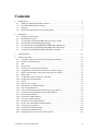
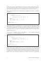
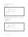
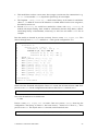
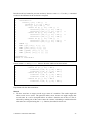
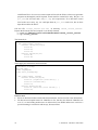
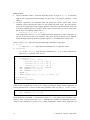
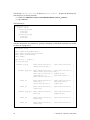
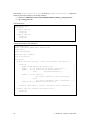
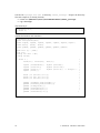
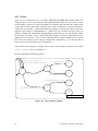
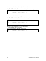
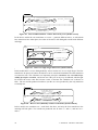
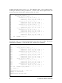
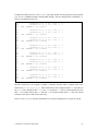
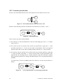
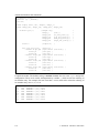
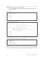
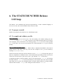
oracle to state based tests. A very simple deterministic model is shown below.
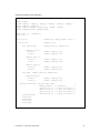
STATECRUNCHER source code
statechart sc
a
α,γ
ab
aa
β
statechart sc(a)
event alpha,beta,gamma;
cluster a(aa,ab)
state aa {alpha,gamma->ab;}
state ab {beta->aa; gamma->aa;}
γ
Figure 1.
A very simple deterministic model and its source code
This model is always in one of two states aa or ab. The initial, or default, state is aa (marked
by the arrow). Transitioning between aa and ab occurs if the model is in state aa and is
given event α or γ to process. Transitioning between ab and aa occurs if the model is in state
ab and is given event β or γ to process. The fact that α and γ are on the same transition in
one direction, but that β and γ are on separate transitions in the other direction, simply shows
flexibility in how the model is written; the effect is the same in cases like this whether the
events are put on the same transition or separate transitions. If the model is in state aa and it
is given event β to process, there is no change in state. Similarly if it is in state ab and it is
© Graham G. Thomason 2003-2004
1
given event α to process. All this behaviour is assumed to be what we require and expect of a
real system: the System Under Test (SUT), also referred to as an Implementation Under Test
(IUT), especially when there may be several implementations of one specified system.
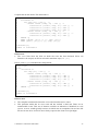
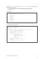
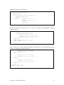
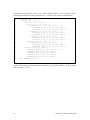
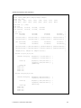
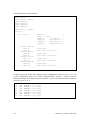
If we compile and run this model, and get the initial configuration (with the gc command),
the output is :
SC:gc
2
statechart sc
2
cluster a [sc] = OCC [] **
2
leafstate aa [a, sc] = OCC []
2
leafstate ab [a, sc] = VAC []
2
TRACE =[]
2
TREV [[alpha, [sc]], 0, [], []]
2
TREV [[gamma, [sc]], 0, [], []]
**
outworlds=[2]
number of outworlds=1
The fact that leafstate aa is occupied, and ab is vacant can be seen. The double asterisks
draw attention to occupied states. Cluster a is occupied is because it is the parent of aa and
ab; this will be explained later. The output also shows transitionable events (the TREV lines),
showing that events alpha and gamma will trigger a transition. The rest of the output will be
explained in due course.
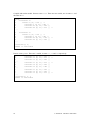
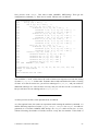
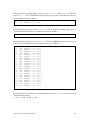
If we now give a command to process event gamma (pe gamma), and then get the new
configuration (gc) , the new configuration is seen:
SC:pe gamma
SC:gc
3
statechart sc
3
cluster a [sc] = OCC [] **
3
leafstate aa [a, sc] = VAC []
3
leafstate ab [a, sc] = OCC []
3
TRACE =[]
3
TREV [[beta, [sc]], 0, [], []]
3
TREV [[gamma, [sc]], 0, [], []]
**
outworlds=[3]
number of outworlds=1
What we have is a tool giving the result of a test - a test oracle. But it is not a test generator
because the user had to decide what event to give STATECRUNCHER to process. Now since
STATECRUNCHER outputs what events it will transition on (and it can also give all its events
on request), one can imagine STATECRUNCHER being connected to another program that
decides on the events to be processed. Such a tool is called a test generator or primer. The
2
© Graham G. Thomason 2003-2004
primer will also pass the events to be tested, and their oracle, to a test harness. The test
harness will (directly or indirectly) call the Implementation Under Test and obtain its new
state, and compare this with the test oracle, and log a pass or fail. This is the basis of
automated test execution.
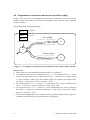
A possible toolset working as described above to go with STATECRUNCHER is TorX [CdR].
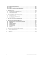
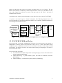
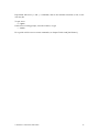
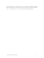
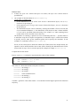
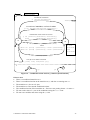
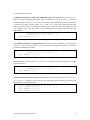
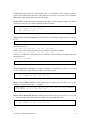
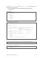
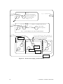
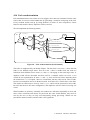
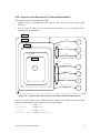
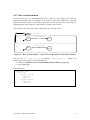
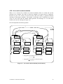
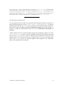
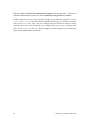
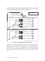
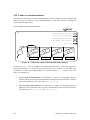
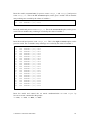
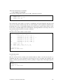
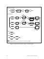
A system to be tested may be a formal component. The following diagram shows the
processes applied to a specification and then a model as it is compiled, validated and deployed
in a testing tool chain such as TorX.
STATECRUNCHER
Component
Specification
Textual
Dynamic
Model
Figure 2.
Compiler/
Validator
Test case
generator
Machine
Engine
Test
harness
Glue
code/
System
Under
Test
Glue
tools
Test
Report
Compilation, Validation and Application to a Testing Tool Chain
1.2 STATECRUNCHER and Prolog
STATECRUNCHER is currently implemented in Prolog. STATECRUNCHER's own syntax is
independent of Prolog, and STATECRUNCHER can be run in a mode that hides Prolog
completely, but it is generally somewhat more convenient to develop a model using a Prolog
environment. The ordinary user does not need to know Prolog as a language at all, however
STATECRUNCHER is run.
STATECRUNCHER can be run:
 As an MS-DOS executable. Apart from a startup message, the user will not be aware
of any connection with Prolog.
 Under SWI-Prolog - a public domain system, (but read the conditions), reference
[SWI-Prolog].
 Under WinProlog - a commercial system, reference [WinProlog].
© Graham G. Thomason 2003-2004
3
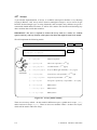
1.3 Notation
UML describes a detailed notation for diagrams, but for historical reasons, (and perhaps also
compactness) this manual differs in respect of certain features:

on entry to a state (UML “entry/”) is a solid triangle pointing in to the state, e.g. v=6

on exit from a state (UML “exit/”) is a solid triangle pointing out of the state, e.g. v=6

events declared in a part of the hierarchy are denoted by the symbol , e.g. ζ1

variables are declared in a part of the hierarchy by the symbol, e.g. v=6

PCOs (Points of Control and Observation) are declared by the symbol , e.g. pco1
1.4 Related documentation by the present author





For the underlying parsing technique: [StCrGP4]
For detail of STATECRUNCHER parsing: [StCrParsing]
For detail of STATECRUNCHER system and design: [StCrMain]
For detail of the STATECRUNCHER-primer protocol: [StCrPrimer]
For test models: [StCrTest]
This manual is self-sufficient as a basic tutorial without reference to other documentation, but
references will be given for amplification on the material in many instances.
4
© Graham G. Thomason 2003-2004
2. Installation
2.1 Hardware requirements
The supported platforms are Windows 98 and above. The disk usage is about 20MB (though
this includes much test material and can be pruned away to about 1 MB).
STATECRUNCHER will run on older, slower machines, but the following will be noticed:
 run-time response for deterministic models will still be fast, by human standards at least.
 run-time response time when there are many worlds in existence will be slow.
 compile time for models with long statements will be noticeably slow.
STATECRUNCHER compilation of models runs rather slowly on a 120 MHz laptop, runs
adequately on a 300 MHz machine (on which it was largely developed), and runs all the better
on more modern machines. There will always be a performance bottleneck under highly
nondeterministic situations, since there is potential for combinatorial explosion. If possible,
keep the number of worlds that models generate to below, say, 100.
2.2 Installation overview
There are various implementations of STATECRUNCHER:
 As an MS-DOS executable, using an embedded WinProlog kernel. Apart from a
startup message, the user will not be aware of any connection with Prolog.
 Under SWI-Prolog - a public domain system, (but read the conditions), reference
[SWI-Prolog].
 Under WinProlog - a commercial system from Logic Programming Associates (LPA),
reference [WinProlog].
There is also a special socket version under SWI-Prolog, (not relevant to a learner), described
in section 5.
In order to run STATECRUNCHER under SWI-Prolog or WinProlog, you need the
STATECRUNCHER source. The MS-DOS executable does not need a Prolog system or the
STATECRUNCHER source.
All versions work with the same modelling language and the same command language though
there are some alternative ways of working, e.g. modelname mode, which are not available in
the MS-DOS executable version). The executable runs in an MS-DOS window, which has the
© Graham G. Thomason 2003-2004
5
disadvantage that is may not be scrollable. It is possible, however, under later versions of
Windows, to set an MS-DOS window to more than the default 24 lines.
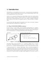
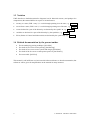
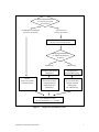
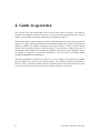
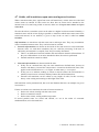
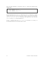
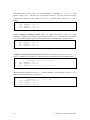
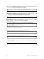
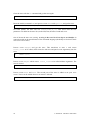
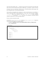
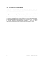
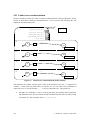
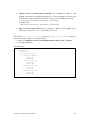
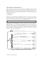
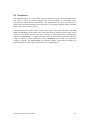
We consider installation of SWI-Prolog and of each STATECRUNCHER system, taking the
process as far as starting up STATECRUNCHER and obtaining a STATECRUNCHER command
prompt ( SC: ). After this stage, the difference between the systems becomes largely
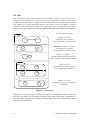
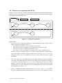
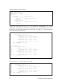
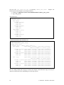
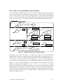
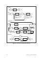
irrelevant. Follow a path in the tree below according to your way of working.
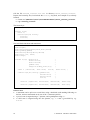
6
© Graham G. Thomason 2003-2004
What implementation
of STATECRUNCHER
do you have?
An MS-DOS executable
of STATECRUNCHER
The source of
STATECRUNCHER
Follow instructions on installation
of STATECRUNCHER source
What implementation
of PROLOG will you
be using?
WinProlog
Follow
STATECRUNCHER
run instructions
SWI-Prolog
Purchase and Install
WinProlog
Download and
Install SWI-Prolog
Follow
STATECRUNCHER
compile and run
instructions for
WinProlog
Follow
STATECRUNCHER
compile and run
instructions
for SWI-Prolog
You should now have
STATECRUNCHER's SC: prompt
Figure 3.
© Graham G. Thomason 2003-2004
Diagram of installation routes
7
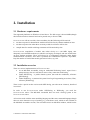
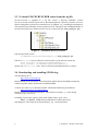
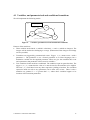
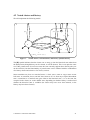
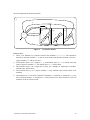
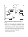
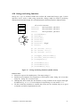
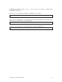
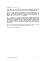
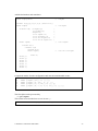
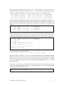
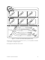
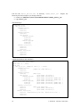
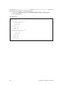
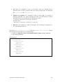
2.3 To install STATECRUNCHER source from the zip file
STATECRUNCHER is supplied in a zip file. Create a directory KWinPro. Extract
STATECRUNCHER from the zip file into it; that should generate a directory structure at least as
shown, (though there will be more subdirectories if supplied, e.g. containing documentation).
The structure below KWinPro is best regarded as fixed. The path to and including KWinPro is
not fixed and can be user defined (in a STATECRUNCHER loader file, aux_load_sc.pl).
Figure 4.
Installation directory structure
Edit (the equivalent to) file
P:\KWinPro\StCr\StCr2Sand\Boot_sc\aux_load_sc.pl
Edit the boot_root lines to reflect the actual location in your directory hierarchy
boot_root(gp4,'P:\Kwinpro\GP4\GP4Sand1\').
boot_root(sc, 'P:\Kwinpro\StCr\StCr2Sand\').
(Ignore any xxboot_root lines - they are effectively disabled and have no effect).
2.4 Downloading and installing SWI-Prolog
The SWI Prolog site is:
http://www.swi-prolog.org/
Read and heed the license details. Do not distribute public domain and Philips proprietary
software together without permission from Philips IP&S.
Versions at or above 5.0.3 should be suitable. Download SWI-Prolog for Windows:
SWI-Prolog/XPCE for MS-Windows
Install as instructed with standard options. This includes accepting .pl as the Prolog
extension (sorry, Perl users).
Preferably, increase the capacity of the main window with regedit. Go to
HKEY_CURRENT_USER\Software\SWI\Plwin\Console\SaveLines
and change the value from 0xc8 (200 decimal) to, say, 0x1f4 (500 lines).
8
© Graham G. Thomason 2003-2004
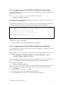
2.5 To compile and run STATECRUNCHER under SWI Prolog
It is assumed that STATECRUNCHER source has been installed as instructed, and that SWIProlog has been installed.
In the StCr\StCr2Sand\boot directory, double click on the file
boot_sc_swipro_win.pl
STATECRUNCHER is recompiled by SWI-Prolog every time it is started up. This only takes a
few seconds on a modern machine.
First SWI Prolog should start up, then STATECRUNCHER will be boot loaded (many files will
be loaded), and you should end up with the following (details may differ slightly):
%
%
F:\KWinPro\StCr\StCr2sand\va_sc\zva_sc.pl compiled 0.00 sec, 4,888 bytes
F:\KWinPro\StCr\StCr2sand\zt_sc\zt_sc_1.pl compiled 0.00 sec, 1,136 bytes
Boot load complete. Prolog system=swiprolog
% aux_load_sc.pl compiled 3.89 sec, 3,638,548 bytes
STATECRUNCHER (Version 1.05)
Copyright (C) Philips Electronics N.V., 2000-2003
SC:
To exit:
 At the SC: prompt, enter quit
 Close the Window (or, in good Prolog tradition, type halt.).
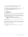
2.6 To compile and run STATECRUNCHER under WinProlog
It is assumed that STATECRUNCHER source has been installed as instructed, and that
WinProlog has been installed.
Start up WinProlog, e.g. using a short cut, with the following command and parameters (read
as one line):
"D:\Program Files\WIN-PROLOG-4010\PRO386W.EXE" /B512
/L1024 /P50000 /H3000 /T1024
This is a considerable amount of memory, and the startup may be slow (a few minutes) on an
older (say, 1998) computer, but once WinProlog has started up, it will perform well.
Open (under the File button)
boot_sc_winpro_win.pl
in the StCr\StCr2Sand\boot directory, and Compile it (under the Run button). Then
minimize the boot_sc_winpro_win.pl window, and in the console window, type
?- cruncher.
This will give STATECRUNCHER's SC: prompt.
 To exit STATECRUNCHER, enter quit (without a full stop).
 To exit WinProlog, select File, Exit, or close the application window.
© Graham G. Thomason 2003-2004
9
2.7 To run the STATECRUNCHER MS-DOS executable
Extract the Zip file into a directory of suggested name KWinPro.
If the full STATECRUNCHER development directory tree has been supplied, then the executable
and related files are to be found in the directory equivalent to
P:\KWinPro\StCr\StCr2Sand\BOOT_SC\StCrExe-Re105
Otherwise, they are in the top level directory.
The executable is
statecruncher.exe
It must be collocated with
statecruncher.ovl
Do not just double click on statecruncher.exe. It must be run with the parameters
specifying memory usage as for WinProlog. The following should be sufficient for most
purposes:
statecruncher.exe /B512 /L1024 /P50000 /H3000 /T1024
Make a shortcut to wherever you put statecruncher.exe on your system. The suggested
parameter settings are made in the shortcut file by right clicking it, selecting properties, and
editing the target to e.g. (read as one line):
F:\KWinPro\StCr\StCr2Sand\BOOT_SC\StCrExeRe105\statecruncher.exe /B512 /L1024 /P50000 /H3000
/T1024
The shortcut can best also be set to start in the current directory, which is set by clearing the
shortcut start in edit box.
This file, when edited as just mentioned, can conveniently be copied to any directory in which
the user is working on a model and used to start it up. (By working this way, the
STATECRUNCHER root command will not be needed). No other files (except the user's
models) are required to run the executable.
When STATECRUNCHER is started up, the prompt
SC:
is given and commands can be entered as described in the report. The command to quit is
SC:quit
10
© Graham G. Thomason 2003-2004
3. Getting started
In this section, we assume that you are able to run STATECRUNCHER and obtain its prompt
( SC: ). It does not matter whether you are using the MS-DOS, SWI-Prolog or WinProlog
variety of STATECRUNCHER.
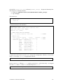
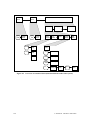
We will make the following model from scratch. It is functionally the same as the model of
section 1.1, but with slightly different naming. Remind yourself of the functionality of the
model from that section. We will call the model
get_started
and put it in directory (adapted for your path)
F:\KWinPro\StCr\StCr5ModelsUser\u5110_get_started
The u5110 naming relates the model to test model t5110, and gives us a convenient
ordering for our models when alphanumerically sorted. The solutions to this manual/tutorial
will be found in directory
F:\KWinPro\StCr\StCr6ModelsTutorial
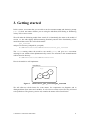
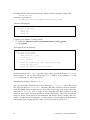
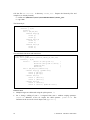
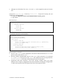
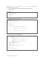
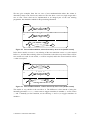
Here is the model we will implement:
statechart sc
a
α,γ
a2
a1
β
γ
Figure 5.
Model u5110_get_started\get_started
We will often use Greek letters for event names, for compactness on diagrams and to
distinguish them from states and variables. In a STATECRUNCHER source file, they will need
to be spelled out. The glossary (section 10) contains the names of the Greek letters.
© Graham G. Thomason 2003-2004
11
We will first implement the state machine hierarchy, without events or transitions. This is
always good practice. Create a file
get_started.scs.txt
in directory (equivalent to)
F:\KWinPro\StCr\StCr5ModelsUser\u5110_get_started
The ending .scs.txt stands for STATECRUNCHER Source. Enter the following text:
statechart sc(a)
cluster a(a1,a2)
state a1;
state a2;
The default state of a cluster is its first member - here a1.
Start STATECRUNCHER and enter (adapting to your path)
SC:root F:\KWinPro\StCr\StCr5ModelsUser\u5110_get_started
SC:cp get_started
Note: If you are using the MS-DOS version of STATECRUNCHER and put a shortcut in the
same directory as the get_started.scs.txt file, you do not need the first command
above.
As long as you are working in the same directory, correcting and refining your model, with
the same invocation of STATECRUNCHER, you will not need to repeat the root command
when you recompile.
The listing that appears on the screen is also available in two parts, in two files that are
created in the same directory as the source file:
get_started.scl.txt
get_started.scv.txt
Observe in passing that two other files are created:
get_started.sco.pl
get_started.scd.pl
These are the compiled model, as PROLOG code, for use by the STATECRUNCHER engine.
The first file contains a basic structural parse of the model, and the second file contains a
symbol table, cross-reference table, and data store.
On compilation, there should be no errors, and one warning, that state a2 is unreferenced.
This can be ignored. If there are errors, check your source code carefully.
It is worth experimenting with a deliberate error, say calling state a2 "a3", or omitting it
altogether. You will get a machine path error. This means that there is a problem that the
states a1 and a2, declared in cluster a(a1,a2), are not found in the expected place.
12
© Graham G. Thomason 2003-2004
Now add the events and transitions. You can also add comments as shown, with // applying to
the rest of the line, as in C++, and /*...*/ enclosing a comment as in C.
Statements of code can be split across more than one line by ending the line with \ (as in
Unix shell commands), but in our model the separate statements (event declarations, state
declarations etc.) easily fit on one line. Do not put two statements on one line.
// My first model
statechart sc(a)
event alpha,beta,gamma;
cluster a(a1,a2)
state a1 {alpha,gamma->a2;}
state a2 {beta->a1; gamma->a1;}
Compile this model. You only need the root command if you have a new invocation of
STATECRUNCHER.
SC:root F:\KWinPro\StCr\StCr5ModelsUser\u5110_get_started
SC:cp get_started
The screen output (also written to the files mentioned) is a compiler listing, and a symbol and
cross reference table. An entry such as
SYMB gamma
[sc]
XREF leafstate
XREF leafstate
eventdecl
[]
a1:[a,sc]
a2:[a,sc]
identifies symbol gamma in statechart scope ( [sc] ), as an event ( eventdecl ) at an
unnamed ( [] ) Point of Control and Observation, and is referenced ( XREF ) in leafstates a1
and a2, both in cluster a scope ( [a,sc] ). Scopes and Points of Control and Observation
will be described later.
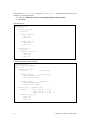
We are now in a position to run the model, getting the configuration and processing events.
If you have previously compiled the model, but are in a new invocation of S TATECRUNCHER,
enter
SC:root F:\KWinPro\StCr\StCr5ModelsUser\u5110_get_started
SC:run get_started
If you have just compiled the model is ready for the next command.
© Graham G. Thomason 2003-2004
13
To see the initial state of the machine, enter
SC:gc
This stands for get configuration. The output is
SC:gc
2
statechart sc
2
cluster a [sc] = OCC [] **
2
leafstate a1 [a, sc] = OCC []
2
leafstate a2 [a, sc] = VAC []
2
TRACE =[]
2
TREV [[alpha, [sc]], 0, [], []]
2
TREV [[gamma, [sc]], 0, [], []]
**
outworlds=[2]
number of outworlds=1
As explained in section 1.1, we see the state occupancies (occupied and vacant). The parent of
states a1 and a2 is cluster a. Only one child state of a cluster can be occupied, and if it is, the
cluster is occupied. If no child states are occupied, the cluster is not occupied. This explains
why cluster a is also occupied. The current configuration has two transitionable events,
alpha and gamma. Since they are in statechart scope ( [sc] ), they can be entered without
scope in the next command we will give. The remaining items of output will be explained as
the subject matter arises throughout this manual.
To process event alpha, enter
SC:pe alpha
The command has completed when a new prompt is given. Follow it up with the get
configuration command.
SC:gc
The output is
SC:gc
3
statechart sc
3
cluster a [sc] = OCC [] **
3
leafstate a1 [a, sc] = VAC []
3
leafstate a2 [a, sc] = OCC []
3
TRACE =[]
3
TREV [[beta, [sc]], 0, [], []]
3
TREV [[gamma, [sc]], 0, [], []]
**
outworlds=[3]
number of outworlds=1
State a1 is now vacant, and state a2 is occupied. The transitionable events have changed.
14
© Graham G. Thomason 2003-2004
Experiment with more pe and gc commands, and see the machine transition (or not, as the
case may be).
To quit, enter
SC:quit
If this leaves a Prolog prompt, close the window, or type
?- halt.
For a guide to all STATECRUNCHER commands, see chapter Table 4 and [StCrPrimer].
© Graham G. Thomason 2003-2004
15
4. Guide to operation
This section covers the functionality of STATECRUNCHER feature by feature. The reader is
assumed to be familiar with the concept of a STATECRUNCHER statechart from the previous
chapter. All statecharts in the following models are implicitly called "sc".
The model numbers as used in directory names in the following sections are of the type unnnn
(where n is a digit) and run in parallel to the test model numbers tnnnn, which are described in
[StCrTest]. Where the numbers correspond, the subject matter is similar, but the tutorial
model is not necessarily identical to the test model - it will often be simpler. The order of
presentation in this manual is not completely sequential with respect to these numbers, since it
is regarded as important to present the material in a the best order for learning, whilst
retaining established model numbering.
The tutorial models are identified for short as a "unnnn" model for convenience, but unlike
the test models, they cannot be run under this name - all it means is that they are found in a
directory unnnn_something and they must be compiled and run using the actual name of the
source file, which is what a user must always do when creating a new model.
16
© Graham G. Thomason 2003-2004
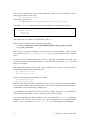
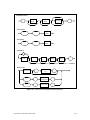
4.1 Variables, and parameterised and conditional transitions
We will implement the following model:
a
b,v1,v2
α(b)[b]
a2
β
α(b)[!b]
a1
γ(v1,v2)[v1>v2]
Figure 6.
a3
Variables, parameterised and transitional conditions
Features of the model are:
 Three variables are declared: b (which is a boolean), v1 and v2 (which are integers). The
integers will be declared as belonging to a range. (Enumerated value integers and strings
are also possible).
 Transitions are triggered by parameterised events. Trigger α(b) means event α with a
parameter b. The parameter is not a formal parameter as in other languages, but a
destination variable for the supplied parameter. When we give the transition this event
and a parameter, that parameter will be stored in variable b.
 Two transitions in this model are conditional. The condition is put in square brackets. The
trigger α(b)[b] means that the value of b must be true for the transition to be eligible.
The term [b] could have been any other expression yielding a boolean. The condition
expression need not refer to any parameters, but it often will, as here. There is also a
transition on gamma if v1 is greater than v2, where these variables happen to be
locations of the transition parameters.
© Graham G. Thomason 2003-2004
17
First implement the state machine hierarchy, without events or transitions. Create a file
param.scs.txt
in directory (equivalent to)
F:\KWinPro\StCr\StCr5ModelsUser\u5123_param
Enter the following text :
statechart sc(a)
cluster a(a1,a2,a3)
state a1;
state a2;
state a3;
Compile it (as in Chapter 3, Getting started).
SC:root F:\KWinPro\StCr\StCr5ModelsUser\u5123_param
SC:cp param
Then upgrade it to the following:
statechart sc(a)
event alpha,beta,gamma;
cluster a(a1,a2,a3)
enum int10 {0,..,10};
int10 v1,v2;
bool b=false;
state a1 {alpha(b)[b]->a2; alpha(b)[!b]->a3;}
state a2 {beta->a3;}
state a3 {gamma(v1,v2)[v1>v2]->a1;}
See how our integer type, int10, specifies a range. Having specified the type (int10), we
declare integers v1 and v2. The boolean type bool is built-in, as are constants true and
false (equivalent to 1 and 0 respectively).
We arbitrarily initialise b, but not v1 or v2.
The type and integer declarations have been declared at cluster a scope. They could
have been put after the statechart statement; then they would have been at statechart
scope. We address these variables in a very local scope, in the scope of the source state of the
transitions, i.e. in a1, a2 and a3 scopes. It does not matter that these variables were not
defined in these scopes. Variables declared in ancestors of the place where they are used will
always be found. An outbound search mechanism will find the nearest variable. But if we
declare a variable deep in the hierarchy, we cannot address it from higher up in the hierarchy
without using some scoping operators. There is more on scoping in section 4.12.
18
© Graham G. Thomason 2003-2004
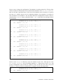
Run the model and get the initial configuration
SC:run param
SC:gc
This should be:
SC:gc
2
statechart sc
2
cluster a [sc] = OCC [] **
2
leafstate a1 [a, sc] = OCC [] **
2
leafstate a2 [a, sc] = VAC []
2
leafstate a3 [a, sc] = VAC []
2
VAR INTEGER b [a, sc] =0
2
VAR INTEGER v1 [a, sc] =unknown
2
VAR INTEGER v2 [a, sc] =unknown
2
TRACE =[]
2
TREV [[alpha, [sc]], 1, [[r, 0, 1]], []]
outworlds=[2]
number of outworlds=1
The line
2
TREV [[alpha, [sc]], 1, [[r, 0, 1]], []]
tells us that there is a transitionable event alpha which takes 1 parameter, which takes
values in a range 0 to 1 ([r,0,1] ).
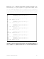
Transition to state ac as follows
SC:pe alpha p=0
SC:gc
This gives us:
SC:gc
3
statechart sc
3
cluster a [sc] = OCC [] **
3
leafstate a1 [a, sc] = VAC []
3
leafstate a2 [a, sc] = VAC []
3
leafstate a3 [a, sc] = OCC [] **
3
VAR INTEGER b [a, sc] =0
3
VAR INTEGER v1 [a, sc] =unknown
3
VAR INTEGER v2 [a, sc] =unknown
3
TRACE =[]
3
TREV [[gamma, [sc]], 2, [[r, 0, 10], [r, 0, 10]], []]
outworlds=[3]
number of outworlds=1
© Graham G. Thomason 2003-2004
19
Now transition to a1 as follows
SC:pe gamma p=[3,2]
SC:gc
The output is:
SC:gc
4
statechart sc
4
cluster a [sc] = OCC [] **
4
leafstate a1 [a, sc] = OCC [] **
4
leafstate a2 [a, sc] = VAC []
4
leafstate a3 [a, sc] = VAC []
4
VAR INTEGER b [a, sc] =0
4
VAR INTEGER v1 [a, sc] =3
4
VAR INTEGER v2 [a, sc] =2
4
TRACE =[]
4
TREV [[alpha, [sc]], 1, [[r, 0, 1]], []]
outworlds=[4]
number of outworlds=1
Note that v1 and v2 now have values.
Experiment by transitioning to state ab on event alpha by providing a parameter value of 1
(=true).
To quit, enter
SC:quit
If this leaves a Prolog prompt, close the window, or type
?- halt.
Remark on enumerated integers with tagnames:
Although not used in these examples, an integer type can be declared with tagnames as
follows:
enum colour
{red,green=3,blue};
Actual integral values are assigned as in C. After the declaration, the symbols red, green
and blue can be used in expressions.
20
© Graham G. Thomason 2003-2004
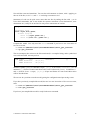
4.2 Nested cluster and history
We will implement the following model:
γ3
x
β3
b
β4
β5
γ4
H
β6
ζ
β7
β8
ζ
α
η
a
η
θ
θ
α
b1
δ5
b2
δ6
δ7
δ8
ω
{deep_clear(x);}
Figure 7.
Nested cluster, self transitions, and history [model u5130]
The (H) symbol indicates that the cluster can on entry go into the historical state rather than
the default state (though history can be cleared, as will be shown). This is not quite the same
as a UML pseudo-state: STATECRUNCHER does not currently support these directly (they are
on the wish-list), but the functionality of pseudo-states can be imitated with the combination
of a history cluster and selective clear history actions.
Some transitions are from or to non-leaf states, i.e. their source states or target states are not
leaf states. A transition from a non-leaf state counts as if it is from any occupied descendant
state. A transition to a non-leaf state goes either to the historical state (i.e. to the state last
occupied in the cluster) or to the default state, depending on whether history is marked and
whether the historical state is available (the cluster may have never been entered, or the
history may have been cleared).
© Graham G. Thomason 2003-2004
21
Call the file nested_cluster.scs.txt in directory u5130_nested_cluster.
Prepare the hierarchy first, but include the history keyword, and compile it (as already
learned).
SC:root F:\KWinPro\StCr\StCr5ModelsUser\u5130_nested_cluster
SC:cp nested_cluster
The hierarchy is:
statechart sc(x)
cluster x(a,b)
state a;
cluster b(b1,b2) history
state b1;
state b2;
Now add the declarations and transitions:
statechart sc(x)
event alpha;
event beta3,beta4,beta5,beta6,beta7,beta8;
event gamma3,gamma4;
event delta5,delta6,delta7,delta8;
event zeta, eta, theta;
event omega;
cluster x(a,b) {beta3->x.a;
beta5->x.b.b1;
beta7->x.b.b2;
gamma3->x.b;
omega->x.a{deep_clear(x);};
state a { beta4->$x;
zeta->b.b2;
eta->b;
cluster b(b1,b2) history {gamma4->$x;
delta5->b.b1;
delta7->b.b2;
eta->a;
\
\
\
\
}
theta->b.b1; }
\
\
\
}
state b1 {alpha->b2;
beta6->$$x;
delta6->$b;
theta->$a;}
state b2 {alpha->b1;
beta8->$$x;
delta8->$b;
zeta->$a;}
Points to note
 A statement can be split over several lines using a backslash (with nothing following on
the line, and not commented out by use of the // comment symbol).
 A parent state is targeted using a $ operator, and a grandparent using $$.
 A child state is targeted using the dot operator, e.g. x.a and a grandchild by e.g.
x.b.b1 .
22
© Graham G. Thomason 2003-2004

This model does not have cousin states, but to target a cousin state, the construction is e.g.
$a.a1 - see test model t5130, depicted in [StCrTest], for an example.
The fragment {deep_clear(x);}, which clears history in all clusters in and below
cluster a, is called an action on the transition. A similar kind of action is an assignment,
described in section 4.6.
Instead of history, we could have marked the cluster with deep history. In
models with deeper nesting, there would be a distinction, because deep history clusters
would keep history of descendants, recursively, as well. See test model t5200 for an
example.


Run the model (as learned in previous sections). Process events eta, alpha, eta. This
takes us through states a, b1, b2, and back to a. Then get the configuration. It is:
SC:gc
5
statechart sc
5
cluster x [sc] = OCC [] **
5
leafstate a [x, sc] = OCC [] **
5
cluster b [x, sc] = VAC b2
5
leafstate b1 [b, x, sc] = VAC []
5
leafstate b2 [b, x, sc] = VAC []
5
TRACE =[]
5
TREV [[beta4, [sc]], 0, [], []]
5
TREV [[zeta, [sc]], 0, [], []]
5
TREV [[eta, [sc]], 0, [], []]
5
TREV [[theta, [sc]], 0, [], []]
5
TREV [[beta3, [sc]], 0, [], []]
5
TREV [[beta5, [sc]], 0, [], []]
5
TREV [[beta7, [sc]], 0, [], []]
5
TREV [[gamma3, [sc]], 0, [], []]
5
TREV [[omega, [sc]], 0, [], []]
outworlds=[5]
number of outworlds=1
Observe the line formatted in bold print. Cluster b is vacant, but its historical state is b2. Now
process event eta. Get the configuration and observe that state b2 is entered, not b1.
6
leafstate b2 [b, x, sc] = OCC []
**
Now reset the machine to its default state
SC:rm
Process events eta, alpha, eta. as before. But now process omega, observing the
configuration. The history of cluster b has been cleared, - instead of b2 there is[]. Now
process event eta. The default state b1 is entered, not the historical state.
8
leafstate b1 [b, x, sc] = OCC []
© Graham G. Thomason 2003-2004
**
23
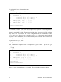
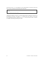
4.3 Sets
Sets, like clusters, have members (which can be leafstates, clusters or sets). But if a set is
occupied, all its members are occupied. The cluster rule applies to members: if one of the
members is a cluster, and it is occupied, then only one member of the cluster will be occupied.
Sets enable us to model parallelism, and we may speak of the set members as parallel
machines. A set can have deep history. The symbol for a set is a rounded box with a tab on
the top left for the set name. The following diagram shows how set members may be depicted.
Note deep history marker
D
s
a
aa
b
ba
ab
member is a cluster
(containing two leafstates)
note symbol a in the member area
alternative: member is a cluster
(containing two leafstates)
note no symbol outside the cluster
bb
member is a leafstate
note no symbol outside the leaf state
(can be useful for self transition actions)
c
d
da
member is a set
(containing two clusters, each of
which contains two leafstates)
daa
dab
dba
dbb
db
e
ea
eaa
eab
Figure 8.
member is a cluster
(containing a cluster (containing two
leafstates))
Set members
Transitions to sets may specify several specific target states in different members, or they may
omit some (in which case the default or historical state will be taken where appropriate), or
they may simply target the set, in which case all the target states will be selected using default
or historical considerations.
24
© Graham G. Thomason 2003-2004
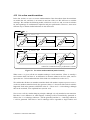
We will implement the following model:
ε
y
β
b
θ
θ
γ
a
γ
b1
b2
q
π
π
p
b3
s
ρ
τ
ρ
r
u
τ
t
δ
Figure 9.
Set [model u5140]
Points to note
 There is no difference in structure between the members b1, b2, b3. The alternative
notation is used for member b1 so that it can be made clear that the transition on event γ
targets member b1, and not just set b.
 The transition from a on β targets b1.q (a nondefault state), b3.t (a default state), but
omits a target for member b2. The default state b2.r will be taken.
 The transition from a on θ targets the set only, not a member or anything in a member.
Default states will be taken.
 The transition from a on γ targets member b1 only. Default states will be taken in all
members.
 The transition on ε exits from a child of set member b3 explicitly. A transition on γ exits
from a nonleaf member. A transition on θ exits from the set as such. In all these cases, all
members of the set will be exited.
© Graham G. Thomason 2003-2004
25
Call the file set.scs.txt in directory u5140_set. Prepare the hierarchy first and
compile it (as already learned).
SC:root F:\KWinPro\StCr\StCr5ModelsUser\u5140_set
SC:cp set
The hierarchy is:
statechart sc(y)
cluster y (a,b)
state a;
set b (b1,b2,b3)
cluster b1(p,q)
state p;
state q;
cluster b2(r,s)
state r;
state s;
cluster b3(t,u)
state t;
state u;
Now add the declarations and transitions:
statechart sc(y)
event beta,gamma,delta,epsilon,theta,pi,rho,tau;
cluster y (a,b)
state a
{beta-> b.(b1.q/\b3.t);
delta->b.(b1.q/\b2.r/\b3.u);
gamma->b.b1;
theta->b;
set b (b1,b2,b3) {theta->a;}
cluster b1(p,q) {gamma->$a;}
state p {pi->q;}
state q {pi->p;}
cluster b2(r,s)
state r {rho->s;}
state s {rho->r;}
cluster b3(t,u)
state t {tau->u;}
state u {tau->t; epsilon->$$a;}
\
\
\
}
Points to note
 Multiple targets are addressed using the split operator, /\.
 Set b, being a sibling of state a, is targeted from state a without scoping operators:
theta->b. Members of the set require the child operator: gamma->b.b1. The
leafstates in the set are all a level deeper still, e.g. b.b1.q.
26
© Graham G. Thomason 2003-2004
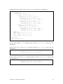
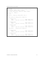
Run the model (as learned in previous sections). Process event beta. Use the gc command
to observe the leafstates in the set that are occupied:
SC:gc
3
statechart sc
3
cluster y [sc] = OCC [] **
3
leafstate a [y, sc] = VAC []
3
set b [y, sc] = OCC [] **
3
cluster b1 [b, y, sc] = OCC []
3
leafstate p [b1, b, y, sc] =
3
leafstate q [b1, b, y, sc] =
3
cluster b2 [b, y, sc] = OCC []
3
leafstate r [b2, b, y, sc] =
3
leafstate s [b2, b, y, sc] =
3
cluster b3 [b, y, sc] = OCC []
3
leafstate t [b3, b, y, sc] =
3
leafstate u [b3, b, y, sc] =
3
TRACE =[]
3
TREV [[pi, [sc]], 0, [], []]
3
TREV [[rho, [sc]], 0, [], []]
3
TREV [[tau, [sc]], 0, [], []]
3
TREV [[gamma, [sc]], 0, [], []]
3
TREV [[theta, [sc]], 0, [], []]
**
VAC
OCC
**
OCC
VAC
**
OCC
VAC
[]
[]
**
[]
[]
**
[]
[]
**
outworlds=[3]
number of outworlds=1
Process events tau and epsilon . Observe how the whole set has been exited:
5
5
5
5
5
5
5
5
5
5
set b [y, sc] = VAC []
cluster b1 [b, y, sc] = VAC q
leafstate p [b1, b, y, sc]
leafstate q [b1, b, y, sc]
cluster b2 [b, y, sc] = VAC r
leafstate r [b2, b, y, sc]
leafstate s [b2, b, y, sc]
cluster b3 [b, y, sc] = VAC u
leafstate t [b3, b, y, sc]
leafstate u [b3, b, y, sc]
= VAC []
= VAC []
= VAC []
= VAC []
= VAC []
= VAC []
Experiment with the other transitions.
Remark
 We have seen how to target several target states of a transition. The reader might ask
about several source states. The question makes sense, because we might require that
several states in a set be occupied before we allow a transition out of the set. This is
achieved by making one of the source states the “master” and adding a condition that the
other states are occupied using the in() function, described in section 4.9.
© Graham G. Thomason 2003-2004
27
4.4 Fired events
Events may be supplied by the user, with the pe command, or they may be generated in the
model, by an action which we call firing an event.
As with user-supplied events, fired events can take parameters.
We illustrate fired events in two contexts
 Where a transition in one part of a machine fires an event which will be responded to in a
parallel part of the machine to cause a transition there.
 An engagement between two parallel parts of a machine representing S TATECRUNCHER's
client-server paradigm. This is considered in the next section (4.5).
Other aspects to fired events, for which we refer the interested reader to test models, are:
 A simple knock-on effect in a machine with no parallelism (see test model t5152).
 Fired events can also be used to generate loops (see test model t5240).
The model we first implement is as follows:
bv1=true; bv2=false
s
a
γ(bv2)
α{fire β(bv1,bv2)}
a1
a2
α
b
bvp1, bvp2
β(bvp1,bvp2)[bvp1&&(!bvp2)]
b1
b2
β{fire α }
Figure 10. Fired event [model u5150]
Points to note
 The user will initially supply event α, and the system will fire event β. After this, when
we are in states a2 and b2, the user can supply event β, and the system will fire event α.
 We declare two boolean variables, bv1 and bv2, and use them as parameters when we
fire the event β.
 The transition labelled β(bvp1,bvp2)[bvp1&&(!bvp2)] receives the parameters
and puts them in its own locations (bvp1 and bvp2). The initial values of bv1 and bv2
(true and false respectively) will allow the transition on β(bvp1,bvp2) to take place,
because the condition evaluates to true. However, bv2 can be set to any value using the
self-transition on γ, so we can arrange for the condition to evaluate to false.
28
© Graham G. Thomason 2003-2004

Although we will initially fire event β via event α, β can be supplied by the user from the
start.
Call the file fire.scs.txt in directory u5150_fire. Prepare the hierarchy first and
compile it (as already learned).
SC:root F:\KWinPro\StCr\StCr5ModelsUser\u5150_fire
SC:cp fire
The hierarchy is:
statechart sc(s)
set s(a,b)
cluster a(a1,a2)
state a1;
state a2;
cluster b(b1,b2)
state b1;
state b2;
Then add the declarations and transitions:
statechart sc(s)
event alpha,beta,gamma;
bool bv1=true,bv2=false;
set s(a,b)
cluster a(a1,a2)
state a1 {alpha->a2{fire beta(bv1,bv2);}; gamma(bv2);}
state a2 {alpha->a1;}
cluster b(b1,b2)
bool bvp1,bvp2;
state b1 {beta(bvp1,bvp2)[bvp1&&(!bvp2)]->b2;}
state b2 {beta->b1 {fire alpha;};}
Run the model (as learned).
 Process event alpha, get the configuration, and observe that the transition on beta took
place as well as the one on alpha.
 Reset the model (command rm). Process event gamma with a parameter of 1 (command
pe gamma p=1). Now process event alpha. The condition on the receiving transition,
[bvp1&&(!bvp2)], is now false, and that transition does not take place.
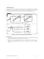
 Experiment with other transitions. Apart from altering variable values, how many
different state occupancy configurations does the model have? Finding the configurations
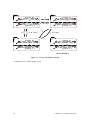
is called exploring the model. The figure below shows the explored model.
© Graham G. Thomason 2003-2004
29
s
a
α{fire β}
a1
b
α
β
b1
α
a2
b2
β{fire α }
β
s
a
a1
b
b1
a1
β - in 2 steps
α - in 3 steps
α{fire β}
α
β
s
a
b
b1
α
β
a2
b2
β{fire α }
α
β - in 3 steps
s
a
a2
b2
α{fire β}
a1
b
b1
β{fire α }
α{fire β}
α
β
a2
b2
β{fire α }
INACCESSIBLE
Figure 11. Fired event model explored
Occupied states are shown shaded, in red.
30
© Graham G. Thomason 2003-2004
4.5 Client-server composition and PCOs
In this section, we see how to model one software component or function calling another,
using fired events. We introduce the concept of PCOs: Points of Control and Observation. We
will implement the following model:
comp
pco_comp
pco_ext
α /fire β
client
C1
server
return
C2
C3
β/fire return
S1
S2
Figure 12. Component composition
Points to note
 STATECRUNCHER's composition paradigm is closely analogous to the function call and
return of imperative languages such as ‘C’.
 The making of the function call is modeled by a fired event
 The response to this is modeled by a transition on the event that was fired
 The return statement is modeled by fired return event
 The response to this is modeled by a transition on the return event that was fired.
If there are many such calling sequences in a model, return names can be made unique to
a server function by affixing the function name to the event (e.g. return_max) or by
putting the return event in a sufficiently local scope (using S TATECRUNCHER's scoping
capabilities.

The client can be seen as an independent state machine, which can be driven through its
cycle with events alpha and return. It does not care who it is that responds to its firing of
β, nor who it is that provides the return event. A different server to the one shown
might be connected to the client, e.g. with more states and transitions between its initial
and final states (S1 an S2). Similarly the server is independent of its client, except for the
agreed interface of β and return.

Event α is supplied externally to the client and server. Events β and return are part of
the agreed interface between the client and server. We indicate this by putting the events
© Graham G. Thomason 2003-2004
31
on different PCOs. STATECRUNCHER's output will reveal the PCOs so that a test generator
program can distinguish, and if required, restrict itself to certain PCOs only. We put α on
pco_ext (for external) and β on pco_cmp (for composition). If we had more events
local to the server only, say, we could put them on pco_serv and so on, but we have
kept this model to the basics.
Call the file client_server.scs.txt in directory u5154_client_server.
Prepare the hierarchy first and compile it (as already learned).
SC:root F:\KWinPro\StCr\StCr5ModelsUser\u5154_client_server
SC:cp client_server
The hierarchy is:
statechart sc(comp)
set comp(client, server)
cluster client(C1,C2,C3)
state C1;
state C2;
state C3;
cluster server(S1,S2)
state S1;
state S2;
Then supply the declarations and transitions:
statechart sc(comp)
PCO ext,cmp;
event alpha@ext;
event beta,return@cmp;
set comp(client, server)
cluster client(C1,C2,C3)
state C1 {alpha->C2 {fire beta;}; }
state C2 {return->C3;}
state C3;
cluster server(S1,S2)
state S1 {beta->S2 {fire return;}; }
state S2;
Points to note
 PCOs are declared in their own declaration statements, and are used in event declarations.
 We haven't used capital letters for identifiers so far, but they are allowed. Identifiers are
as in 'C', so non-leading underscores are allowed too, but double underscores can have a
special meaning in connection with arrays, discussed later.
32
© Graham G. Thomason 2003-2004
Compile and run the model. The initial state is:
SC:gc
2
statechart sc
2
set comp [sc] = OCC [] **
2
cluster client [comp, sc] = OCC []
2
leafstate C1 [client, comp, sc]
2
leafstate C2 [client, comp, sc]
2
leafstate C3 [client, comp, sc]
2
cluster server [comp, sc] = OCC []
2
leafstate S1 [server, comp, sc]
2
leafstate S2 [server, comp, sc]
2
TRACE =[]
2
TREV [[alpha, [sc]], 0, [], [ext, [sc]]]
2
TREV [[beta, [sc]], 0, [], [cmp, [sc]]]
**
= OCC []
= VAC []
= VAC []
**
= OCC []
= VAC []
**
**
outworlds=[2]
number of outworlds=1
Point to note
 The TREV lines show the PCO on which the event has been declared. PCOs can
themselves be scoped; our PCOs are both in statechart scope, i.e. [sc].
Process event alpha and obtain the configuration:
SC:pe alpha
SC:gc
5
statechart sc
5
set comp [sc] = OCC [] **
5
cluster client [comp, sc] = OCC []
5
leafstate C1 [client, comp, sc]
5
leafstate C2 [client, comp, sc]
5
leafstate C3 [client, comp, sc]
5
cluster server [comp, sc] = OCC []
5
leafstate S1 [server, comp, sc]
5
leafstate S2 [server, comp, sc]
5
TRACE =[]
**
= VAC
= VAC
= OCC
**
= VAC
= OCC
[]
[]
[]
**
[]
[]
**
outworlds=[5]
number of outworlds=1
Points to note
 The complete transaction between the server and client has run its course.
 This particular model has no reset event and has reached a dead end. There are no
transitionable events. This sort of situation could be an indication of deadlock in a real
system. A server would typically return to its initial state on completion, but we have left
this one in state S2 as we feel it more clearly expresses the client-server paradigm.
© Graham G. Thomason 2003-2004
33
4.6 Assignments on transitions and inexact variable scoping
In this section we show how assignments can be made on transitions. We also show that
variables of the same name can be declared in different scopes; they are then completely
separate variables.
We will implement the following model:
v=1
a
v=2
param
the global v
v
the local v
v
exact scoping
α{$v+=3; $$v=$v+6;}
a2
no very-local v here
γ($param){$v=$param;}
a1
inexact scoping
β{v+=3; $$v=v+6;}
a3
γ(param){v=param;}
Figure 13. Assignment on transition with overloaded variable names [model u5160]
Points to note
 There can be several assignments (and other actions) on a transition.
 An arithmetic expression on a transition such as v+=3 in principle refers to a v in the
scope of the source state. So for a transition from state a1, it refers to a v declared in state
a1 scope. However, if there is no such variable in this scope, which is the situation here,
the nearest v will be used; it is the v in cluster a scope.
 An expression such as $v+=3 refers to a v in the parent scope. So for a transition from
state a1, it refers to a v declared in cluster a scope. This v exists.
 An expression such as $$v+=3 refers to a v in the grandparent scope. So for a transition
from state a1, it refers to a v declared in statechart sc scope. This v exists, and is distinct
from the v in cluster a scope.
 The rule about finding the nearest variable in scope, searching up the hierarchy, applies to
variables on the left hand side or right hand side of expressions.
34
© Graham G. Thomason 2003-2004
Call the file assign.scs.txt in directory u5160_assign. Prepare the hierarchy first
and compile it (as already learned).
SC:root F:\KWinPro\StCr\StCr5ModelsUser\u5160_assign
SC:cp assign
The hierarchy is:
statechart sc(a)
cluster a(a1,a2,a3)
state a1;
state a2;
state a3;
Then supply the declarations and transitions:
statechart sc(a)
event alpha,beta,gamma;
enum int1 {0,..,1000};
int1 v=1;
cluster a(a1,a2,a3)
int1 v=2;
int1 param;
state a1 {alpha->a2 {$v+=3;$$v=$v+6;};
beta->a3 {v+=3;$$v=v+6;};
\
}
state a2 {gamma($param)->a1{$v=$param;}; }
state a3 {gamma(param)->a1{v=param;};
}
Run the model and get the initial configuration:
SC:gc
2
statechart sc
2
cluster a [sc] = OCC [] **
2
leafstate a1 [a, sc] = OCC []
2
leafstate a2 [a, sc] = VAC []
2
leafstate a3 [a, sc] = VAC []
2
VAR INTEGER param [a, sc] =unknown
2
VAR INTEGER v [a, sc] =2
2
VAR INTEGER v [sc] =1
2
TRACE =[]
2
TREV [[alpha, [sc]], 0, [], []]
2
TREV [[beta, [sc]], 0, [], []]
**
outworlds=[2]
number of outworlds=1
© Graham G. Thomason 2003-2004
35
Points to note
 The two variables called v are shown with their scope. A scope of [a,sc] is read from
right to left if we descend in the hierarchy: we get to this v by going to statechart sc and
cluster a.
 Variable expressions are evaluated from the perspective of the source state of the
transition. Note in passing that states are also listed with their scope. We have already
seen how we target states using scoping operators. The issue of states and their scope can
be a little confusing, because a scope is itself a state. Given a state, we say its scope is the
parent state. This explains output such as
leafstate a1 [a, sc] = VAC []
State expressions such as a.b are evaluated from the perspective of the scope part, or
parent, of the source state of a transition. This gives the most natural way to address
states: siblings require no operators, parents require a $, and child states require a dot.
Process event alpha. This will cause the following evaluations to take place
 $v+=3;
$v is the v in [a,sc] scope and was initialized to 2, so it gets the value 5.
 $$v=$v+6;
$$v is the v in [sc] scope and was initialized to 1. $v is as above and has the
value 5. So $$v gets the value 5+6=11.
SC:gc
5
statechart sc
5
cluster a [sc] = OCC [] **
5
leafstate a1 [a, sc] = VAC []
5
leafstate a2 [a, sc] = OCC [] **
5
leafstate a3 [a, sc] = VAC []
5
VAR INTEGER param [a, sc] =unknown
5
VAR INTEGER v [a, sc] =5
5
VAR INTEGER v [sc] =11
5
TRACE =[]
5
TREV [[gamma, [sc]], 1, [[r, 0, 1000]], []]
outworlds=[5]
number of outworlds=1
There is now a transition on event gamma, taking a parameter, which is then assigned to an
exactly specified local v. Process it with some parameter value, say, 88 (pe gamma p=88):
7
7
VAR
VAR
INTEGER param [a, sc] =88
INTEGER v [a, sc] =88
Reset the model (command rm) and process event beta. The effect on the variables is the
same as when we processed event alpha, although one variable was addressed inexactly.
There is also a transition on event gamma, taking a parameter, which is then assigned to an
36
© Graham G. Thomason 2003-2004
inexactly specified local v. The effect is as above, in the exactly specified case. Remember
that we could have placed our parameter directly into variable v, specifying the transition
with γ($v) rather than γ($param), but here we make a copy of the parameter.
© Graham G. Thomason 2003-2004
37
4.7 Orbits, self-transitions, upon-enter and upon-exit actions
When a transition takes place, (apart from some self-transitions), various states are exited and
various states are entered. In this section we show how an action can be attached to the
internal event of a state being exited or entered, which we call upon enter actions and upon
exit actions.
We also show how a transition course can be taken to a higher level than normal. Normally, a
transition course will be as low-flying as possible. A transition which causes more states to be
exited and entered, in our notation, is given a loop in the arc and is called an orbital
transition.
Self transitions are transitions with the same source and target state. They may nevertheless
cause a transition between states. They can be internal or external.
 Internal self-transitions are drawn on the inside of the state and never cause transitions
between states. As with other transitions, they are valid for processing if the state to
which they are attached is occupied; if not, they are totally discounted.
 There is no difference between leafstate and non-leafstate internal self-transitions. If
they are valid and there is an action attached to them, the action is performed.
 Internal transitions cannot be orbital.

External self-transitions are drawn outside the state.
 If they are on a nonleaf state, they can cause transitions to default states, (but not in
clusters with history, because the current state is counted as the historical state). This
applies to the self-transition on ε3 in Figure 14 when state p2 is occupied.
 If they are on a leafstate, nothing is exited or entered (unless the self-transition is
orbital), but actions are executed, and they behave like internal transitions.
 External self transitions can be orbital (to any height of orbit). In this case they
always cause exiting and entering to the height of the orbit.
Self transitions can be parameterised, but we do not illustrate that here; an example was given
in section 4.4.
If there are actions on a transition, the order of action execution is:
1. Do the exit actions, starting with the source state
2. Do the on-transition actions
3. Do the enter actions, ending with the target state.
If several parallel states are exited and entered, we are in the realm of set-transit
nondeterminism, to be discussed later.
38
© Graham G. Thomason 2003-2004
δ/u*=10;v*=10
a
β/
u*=10
v*=10
p
q
β
γ
p2
α
α
u=u*10+5
v=v*10+1
p1
α
q2
γ
q1
α
v=v*10+5
u=u*10+1
v=v*10+5
u=u*10+1
ζ1/w++
unspecifiable
ζ3/w++
v=v*10+4
u=u*10+2
ζ4/w++
u=u*10+5
v=v*10+1
ω{u=0;v=0;w=0;}
ε1{w++;}
unspecifiable
u=u*10+4
v=v*10+2
ε3 {w++;}
ε4 {w++;}
v=v*10+3
u=u*10+3
Figure 14. Orbits, self-transitions, upon-enter and upon-exit actions [model u5170]
Points to note
 We often for compactness will use a shorter notation for events and transition actions:
event/action rather than event{action;}.
 The arrow symbolsand  indicate actions that take place when the state is exited or
entered. Imagine a transition from say, p1 to q1 (which event β could occasion). The
action on exiting p1 is v=v*10+1. This adds a digit 1 to the current value of v. On
exiting state p, we add the digit 2 to the value of v. Each exit or enter action is tracked in
this way. Variable v tracks a transition from p to q. Variable u tracks a transition from q
to p. The on-transition actions simply add digit 0 to u and v by multiplying by 10. This
gives us a complete record of the order of the actions that take place during a transition.
The variables can be reset without any transitioning by executing event ω.
 In addition to assignment actions we can have any other actions, e.g. fired event actions
(not used in this model, but see test model t5170 for an example).
 For more examples of orbits, see test model t6260, which includes an orbit that exits
members of a set without exiting the set itself.
© Graham G. Thomason 2003-2004
39
Call the file orbits.scs.txt in directory u5170_orbits. Prepare the hierarchy first
and compile it (as already learned).
SC:root F:\KWinPro\StCr\StCr5ModelsUser\u5170_orbits
SC:cp orbits
The hierarchy is:
statechart sc(a)
cluster a(p,q)
cluster p(p1,p2)
state p1;
state p2;
cluster q(q1,q2)
state q1;
state q2;
Add the declarations and transitions, (perhaps compiling as individual transitions are added,
to check for typing errors).
statechart sc(a)
event
event
event
event
alpha,beta,gamma,delta;
epsilon1,epsilon3,epsilon4;
zeta1,zeta3,zeta4;
omega;
enum int {0,..,10000};
int u=0,v=0,w=0;
cluster a(p,q)
40
{upon enter{u=u*10+3;}
omega{u=0;v=0;w=0;};
upon exit{v=v*10+3;}
\
}
cluster p(p1,p2) {upon enter{u=u*10+4;}
upon exit{v=v*10+2;}
delta->$$sc->q{u*=10;v*=10;};
beta->q{u*=10;v*=10;}; gamma->q.q2;
epsilon1{w++;};
epsilon3->p{w++;};
epsilon4->$a->p{w++;};
\
\
\
\
}
state p1
{upon enter{u=u*10+5;}
zeta1{w++;};
zeta4->$p->p1{w++;};
upon exit{v=v*10+1;}
zeta3->p1{w++;};
alpha->p2;
\
\
}
state p2
{upon enter{u=u*10+5;}
alpha->p1;
upon exit{v=v*10+1;}
\
}
cluster q(q1,q2) {upon enter{v=v*10+4;}
beta->p;
upon exit{u=u*10+2;}
gamma->p.p2;
\
}
state q1
{upon enter{v=v*10+5;}
alpha->q2;
upon exit{u=u*10+1;}
\
}
state q2
{upon enter{v=v*10+5;}
alpha->q1;
upon exit{u=u*10+1;}
\
© Graham G. Thomason 2003-2004
Points to note
 If there are upon enter actions and upon exit actions, the upon enter actions must be
specified first.
 An example of orbital notation is delta->$$sc->q.
Useful rules on orbital states
 If the transition arc to an orbital state crosses n hierarchical layers, use (n+1) $
characters in specifying it.
 If the transition arc to a target state crosses n hierarchical layers, use (n) $ characters
in specifying it.
 The hierarchical layers can be counted by counting the number of boxes crossed (but
not set member boundaries, i.e. the dotted line). Note, however, that a cluster member
of a set can be specified without drawing a box round it, so when counting boxes
exited, allow for an ‘invisible’ box in this case.
An alternative to counting $ operators is to use an absolute path. The :: operator takes us
to statechart scope, but it requires an argument, so statechart scope is a little inconvenient
to specify, and we must go the statechart parent and re-specify the statechart. In our
example, we could have used delta->::$sc->q.
So far, we have been precise about the orbital state. Where states have unique names, the
operators can be omitted and the correct state will be found by the outbound search for the
nearest state in scope. So we can also specify the example as simply delta->sc->q.
Compile and run the model.
Process event delta and notice in particular the values of the variables
11
11
11
VAR
VAR
VAR
INTEGER u [sc] =3
INTEGER v [sc] =123045
INTEGER w [sc] =0
The value of v shows that actions took place as follows
v=v*10+1 on exiting p1
v=v*10+2 on exiting p
v=v*10+3 on exiting a
v=v*10
as the transition action
v=v*10+4 on entering q
v=v*10+5 on entering q1
Variable u gained its value when cluster a was entered from the highest point in the transition
trajectory.
© Graham G. Thomason 2003-2004
41
Reset the model (command rm) and process event beta. Observe and explain the new
variable values.
9
9
9
VAR
VAR
VAR
INTEGER u [sc] =0
INTEGER v [sc] =12045
INTEGER w [sc] =0
Reset the model and process event alpha, followed by event omega. The state is p2 and the
variables have been reset. Process from this state, resetting as required, the self transitions
epsilon1, epsilon3, epsilon4, observing at each stage the new state. Note that
epsilon3 and epsilon4 cause a transition to p1.
In state p1, experiment with events zeta1, zeta3, zeta4. Note that zeta4 causes p1 to
be exited and re-entered, as is seen by the values of u and v.
42
© Graham G. Thomason 2003-2004
4.8 Meta-events
In the previous section, we saw how to attach actions to the internal event of a state being
exited or entered. This section shows how that the internal events are like any others, and can
be used to trigger transitions. They never take parameters. We call them meta-events.
s
a
α
p
α
q
p2
β
β
β
a1
q2
β
q1
p1
α
b
j
exit($a.a1)
j1
exit($a.p)
j2
enter($a.a1)
j3
b1
γ
Figure 15. Meta event (state entry/exit) [model u5180]
Points to note
 We respond in set member b to meta events in set member a, and address the states with
the usual scoping notation. The initiating event is in each case α.
 Event γ acts as a reset in member b. In state b1 we respond to various meta events we
might see. Having responded to one meta event, we can reset to state b1 and wait for the
next one.
© Graham G. Thomason 2003-2004
43
Call the file meta.scs.txt in directory u5180_meta. Prepare the hierarchy first and
compile it (as already learned).
SC:root F:\KWinPro\StCr\StCr5ModelsUser\u5180_meta
SC:cp meta
The hierarchy is:
statechart sc(s)
set s(a,b)
cluster a(a1,p,q)
state a1;
cluster p(p1,p2)
state p1;
state p2;
cluster q(q1,q2)
state q1;
state q2;
cluster b(b1,j)
state b1;
cluster j(j1,j2,j3)
state j1;
state j2;
state j3;
Add the declarations and transitions:
statechart sc(s)
event alpha,beta,gamma;
set s(a,b)
cluster a(a1,p,q)
state a1
{alpha->p.p2;}
cluster p(p1,p2)
{alpha->q.q2;}
state p1 {beta->p2;}
state p2 {beta->p1;}
cluster q(q1,q2)
{alpha->a1;}
state q1 {beta->q2;}
state q2 {beta->q1;}
cluster b(b1,j) {gamma->b.b1;}
state b1
{exit ($a.a1)-> j.j1;
exit ($a.p) -> j.j2;
enter ($a.a1)-> j.j3;
cluster j(j1,j2,j3)
state j1;
state j2;
state j3;
44
\
\
}
© Graham G. Thomason 2003-2004
Compile and run the model. Process event alpha, and observe the configuration:
SC:gc
4
statechart sc
4
set s [sc] = OCC [] **
4
cluster a [s, sc] = OCC [] **
4
leafstate a1 [a, s, sc] = VAC
4
cluster p [a, s, sc] = OCC []
4
leafstate p1 [p, a, s, sc]
4
leafstate p2 [p, a, s, sc]
4
cluster q [a, s, sc] = VAC []
4
leafstate q1 [q, a, s, sc]
4
leafstate q2 [q, a, s, sc]
4
cluster b [s, sc] = OCC [] **
4
leafstate b1 [b, s, sc] = VAC
4
cluster j [b, s, sc] = OCC []
4
leafstate j1 [j, b, s, sc]
4
leafstate j2 [j, b, s, sc]
4
leafstate j3 [j, b, s, sc]
4
TRACE =[]
4
TREV [[beta, [sc]], 0, [], []]
4
TREV [[alpha, [sc]], 0, [], []]
4
TREV [[gamma, [sc]], 0, [], []]
[]
**
= VAC []
= OCC []
**
= VAC []
= VAC []
[]
**
= OCC []
= VAC []
= VAC []
**
outworlds=[4]
number of outworlds=1
The fact that leafstate j1 is occupied shows that the exit($a.a1) meta-event was
responded to.
Process events gamma and alpha, and observe that the exit($a.p) meta event was
responded to:
7
7
7
leafstate j1 [j, b, s, sc] = VAC []
leafstate j2 [j, b, s, sc] = OCC []
leafstate j3 [j, b, s, sc] = VAC []
**
Process events gamma and alpha again and observe that the enter($a.a1)meta event
was responded to:
10
10
10
leafstate j1 [j, b, s, sc] = VAC []
leafstate j2 [j, b, s, sc] = VAC []
leafstate j3 [j, b, s, sc] = OCC []
© Graham G. Thomason 2003-2004
**
45
4.9 Conditional actions and the in() function
We have already seen (section 4.1) how a transition can be conditional. In this section we will
see how a transition action can be conditional, even if the transition is unconditional. In fact,
any action can be conditional, so an upon entry action or upon exit action can be conditional
too.
Conditions are expressions evaluating to a boolean value. The expression can make use of the
function in(). This function takes a scoped state as an argument (in the same way a
transition target state is expressed), and returns true (=1) if that state is occupied, false (=0)
otherwise. It will normally be testing the occupancy of a state in a parallel part of the
machine. It is evaluated during execution just before the transition is considered for taking
place, and the value of the function at this time might not be the same as at the start of
processing a user event (e.g. if various events have been fired in the meantime).
Conditions on transitions are written in square brackets. Conditional actions use the if
keyword, and can have an else part. There is an if action and (optionally) an else action.
These actions can be assignments, function calls, fired events, or nested if actions.
We will implement the model in the following figure:
46
© Graham G. Thomason 2003-2004
u=0 v=0 w=0
s
a
conditional transition
α [in($z.z2)&&v==0]
setv(v)
unconditional transition, conditional action
β if (in($z.z2)&&v==0){w=w*10+1;}
conditional action with else action
γ if (v%2==1){w=w*10+2; w=w*10+3;}
else
{w=w*10+4; w=w*10+5;}
a1
a2
δ if (v%2==1) {AC1} else {AC2}
where
AC1= if (v==3) {w=w*10+1;} else {w=w*10+2;}
AC2= if (v==4) {w=w*10+3;} else {w=w*10+4;}

if v>5
u=u*10+1
else
u=u*10+2
ε if (v%2==1){fire ζ2;}
reset for next demo-transition
η {u=0; v=0; w=0;fire ζ1;}
z
z1
ζ1
ζ2
z2
Figure 16. Conditional actions and in() function [model u5190]
Points to note
 There is a conditional transition on α.
 There is a conditional action on the transition on β, and also on entering state a2.
 The transition on γ has an else part.
 The transition on δ has nested conditional actions.
 The conditional action of the transition on ε fires an event, putting cluster z in state z2.
 We can set the value of v (use in the conditions) using the setv event.
 We can reset variables and states using the η event.
© Graham G. Thomason 2003-2004
47
Call the file cond_action.scs.txt in directory u5190_cond_action. Prepare the
hierarchy first and compile it (as already learned).
SC:root F:\KWinPro\StCr\StCr5ModelsUser\u5190_cond_action
SC:cp cond_action
The hierarchy is:
statechart sc(s)
set s(a,z)
cluster a(a1,a2)
state a1;
state a2;
cluster z(z1,z2)
state z1;
state z2;
Add the declarations and transitions:
statechart sc(s)
event alpha,beta,gamma,delta,epsilon,eta;
event setv;
event zeta1,zeta2;
enum int1 {0,..,10000};
int1 u=0,v=0,w=0;
set s(a,z)
cluster a(a1,a2) {setv(v);
eta->a.a1 {u=v=w=0; fire zeta1;}; }
state a1
{alpha [in($z.xxx.z2) && (v==0)]->a2;
beta->
a2 {if (in($z.z2) && (v==0)) {w=w*10+1;} };
gamma-> a2 {if (v%2==1) {w=w*10+2;w=w*10+3;}
else
{w=w*10+4;w=w*10+5;} };
\
\
\
\
\
\
delta-> a2 {if (v%2==1)
\
{if (v==3) {w=w*10+1;} else {w=w*10+2;}}
\
else
\
{if (v==4) {w=w*10+3;} else {w=w*10+4;}} }; \
epsilon->a2 {if (v%2==1) {fire zeta2;}};
}
state a2 {upon enter { if(v>5) {u=u*10+1;} else {u=u*10+2;}}
}
cluster z(z1,z2) {zeta2->z.z2; zeta1->z.z1;}
state z1;
state z2;
48
© Graham G. Thomason 2003-2004
Compile and run the model.
Conditional transition (revision) and conditional upon enter action: Process event alpha,
and note that no transition takes place. This is because we are not in state z2, which the
condition requires. (In fact alpha is not even shown as transitionable, because the condition
is known to be false). Process events zeta2 and alpha. This time a transition does take
place, and we are in state a2. When we entered state a2, the else part of a conditional action
was executed, and u got the value 2. The important lines of output showing what has
happened are:
5
5
5
VAR
leafstate a2 [a, s, sc] = OCC []
leafstate z2 [z, s, sc] = OCC []
INTEGER u [sc] =2
**
**
Unconditional transition, conditional action: Reset the model, (command rm) and process
event beta. As we are not in state z2, the action does not take place (variable w remains at
0), but the transition goes ahead.
4
4
4
VAR
leafstate a2 [a, s, sc] = OCC []
leafstate z1 [z, s, sc] = OCC []
INTEGER w [sc] =0
**
**
Reset the model, process events zeta2 and beta. Now the action does take place (variable
w gets the value 1).
6
6
6
VAR
leafstate a2 [a, s, sc] = OCC []
leafstate z2 [z, s, sc] = OCC []
INTEGER w [sc] =1
**
**
Conditional transition action with else action: Reset the model and process event gamma.
As v2=0, (so v2 modulo 2 is also =0), the else action takes place (variable w becomes 45);
the transition goes ahead anyway.
6
6
6
6
VAR
VAR
VAR
leafstate a2 [a, s, sc] = OCC []
INTEGER u [sc] =2
INTEGER v [sc] =0
INTEGER w [sc] =45
© Graham G. Thomason 2003-2004
**
49
Reset the model, process event setv with parameter 7 (command pe setv p=7), and
process event gamma. This time the if action takes place (w gets the value 23), and the
transition goes ahead as usual. Since v is now >6, u gets the value 1 on entry to a2 for a
change.
7
7
7
7
VAR
VAR
VAR
leafstate a2 [a, s, sc] = OCC []
INTEGER u [sc] =1
INTEGER v [sc] =7
INTEGER w [sc] =23
**
Nested conditional transition action: Reset the model and process event setv with
parameter 4 (syntax as given above). Now process event delta. We satisfy the else part of
the outer condition and the if part of the associated inner condition, and w gets the value 3.
6
6
6
6
VAR
VAR
VAR
leafstate a2 [a, s, sc] = OCC []
INTEGER u [sc] =2
INTEGER v [sc] =4
INTEGER w [sc] =3
**
Experiment with other values of v.
Conditional transition action firing an event: Reset the model and process event epsilon,
Since v2 modulo 2 is not equal to 1, the action does not take place and we remain in state z1.
4
4
4
4
4
VAR
VAR
VAR
leafstate z1 [z, s, sc] = OCC [] **
leafstate z2 [z, s, sc] = VAC []
INTEGER u [sc] =2
INTEGER v [sc] =0
INTEGER w [sc] =0z2 [z, s, sc] = VAC []
Reset the model and process event setv with a parameter 1. Now process event epsilon;
the action takes place and we are in state z2.
6
6
6
6
6
50
VAR
VAR
VAR
leafstate z1 [z, s, sc] = VAC []
leafstate z2 [z, s, sc] = OCC []
INTEGER u [sc] =2
INTEGER v [sc] =1
INTEGER w [sc] =0
**
© Graham G. Thomason 2003-2004
4.10 Strings and string functions
Strings are a type of constant/variable like boolean and enumerated integer types. Certain
operators can be used to make string expressions. Strings might be useful in producing
annotated and formatted output. We will implement the following model to illustrate them:
s1="azA"
s2="z"
v=3
a
etc.
all are self- transitions:
sets1(s1)
sets2(s2)
setv(v)
α1
α2
α3
α4
α5
α6
α7
//direct parameter placement
//direct parameter placement
//direct parameter placement
{s1="abcdef";}
{s2="cd";}
{s1=s1+s2;}
{s1=s1-s2;}
{s1=s1*v;}
{s1=s1/3;} //illegal
{s1="";}
β1 {if (s1==s2) {v++;}}
β2 {if (s1>s2) {v++;}}
β3 {if (s1>=s2) {v++;}}
γ1 {s1=upper_case(s1+"aA");}
γ2 {s1=lower_case(s1+"zZ");}
γ3 {v=length(s1);}
γ4 {s1=format(v,0);}
γ5 {s1=format(v,3);}
γ6 {s1=format(v,-3);}
Figure 17. Strings and String Functions [model u5220]
Points to note
 Strings are expressed in double quotes. The empty string is "".
 Strings can be compared. The comparison is on the ASCII values. String "ab" is less than
string "bc". String "ab" is less than "abc".
 Although the above model does not illustrate it, string variables can be scoped, and might
be addressed e.g. as $$s2. For an example of scoped strings, see test model t5520.
 We have drawn the transitions as external, but as they are on a leafstate, they are as good
as internal, and will be implemented as such.
© Graham G. Thomason 2003-2004
51
Call the file strings.scs.txt in directory u5220_strings. Prepare the hierarchy
first and compile it (as already learned).
SC:root F:\KWinPro\StCr\StCr5ModelsUser\u5220_strings
SC:cp strings
The hierarchy is:
statechart sc(a)
state a;
Add the declarations and transitions:
statechart sc(a)
event sets1,sets2,setv;
event alpha1, alpha2, alpha3, alpha4, alpha5, alpha6, alpha7;
event beta1, beta2, beta3;
event gamma1, gamma2, gamma3, gamma4, gamma5, gamma6;
enum int1 {0,..,1000};
int1 v=3;
string s1= "az" + "A";
string s2="z";
state a {
sets1(s1);
alpha1
alpha3
alpha5
alpha7
sets2(s2);
{s1="abcdef";};
{s1=s1+s2;};
{s1=s1*v;};
{s1="";};
\
\
\
\
\
\
\
\
\
\
\
\
\
\
\
\
\
setv(v);
alpha2 {s2="cd";};
alpha4 {s1=s1-s2;};
alpha6 {s1=s1/3;}; /* illegal */
beta1 {if (s1==s2) {v++;}};
beta2 {if (s1> s2) {v++;}};
beta3 {if (s1>=s2) {v++;}};
gamma1
gamma2
gamma3
gamma4
gamma5
gamma6
52
{s1=upper_case(s1+"aA");};
{s1=lower_case(s1+"zZ");};
{v=length(s1);};
{s1=format(v,0);};
{s1=format(v,3);};
{s1=format(v,-3);};
}
© Graham G. Thomason 2003-2004
Compile the model. Ignore the warning that state a is unreferenced. The warning would not
appear if the leafstate were the first or only leafstate in a cluster or set, but here it is somewhat
abnormally in the statechart directly. Run the model.
String values: Obtain the initial configuration and observe how strings are output. The ASCII
values are printed in a list, and the printable characters follow.
2
2
2
VAR
VAR
VAR
STRING s1 [sc] =[97, 122, 65] =azA
STRING s2 [sc] =[122] =z
INTEGER v [sc] =3
Setting strings in event parameters: Transitionable events taking string parameters are shown
by e.g.
2
TREV [[sets1, [sc]], 1, [[<string>]], []]
Process event sets1 with a parameter of string "aAzZ". The formal way to do this is to give
the following (try it):
pe sets1 p=[[ex_str, [97, 65, 122, 90]]]
If there were several more parameters, they would be inserted at the ellipsis:
pe sets1 p=[[ex_str, [97, 65, 122, 90]],...]
However, provided the string looks like an identifier, the following is accepted (reset the
model and try it).
pe sets1 p=aAzZ
3
VAR
STRING
s1 [sc] =[97, 65, 122, 90] =aAzZ
String assignment on transition: A simple assignment is illustrated by events alpha1 and
alpha2. Reset the model and process these two events, giving:
6
6
VAR
VAR
STRING
STRING
s1 [sc] =[97, 98, 99, 100, 101, 102] =abcdef
s2 [sc] =[99, 100] =cd
Strings can be added: Without resetting after the last events, process event alpha3. The
strings are concatenated by the "+" operator:
8 VAR STRING
8 VAR STRING
s1 [sc] =[97, 98, 99, 100, 101, 102, 99, 100] =abcdefcd
s2 [sc] =[99, 100] =cd
Strings can be subtracted: Without resetting after the last events, process event alpha4. The
"-" operator removes the first occurrence of the second operand in the first:
10
10
VAR
VAR
STRING
STRING
s1 [sc] =[97, 98, 101, 102, 99, 100] =abefcd
s2 [sc] =[99, 100] =cd
© Graham G. Thomason 2003-2004
53
Strings can be multiplied by a constant: Without resetting after the last events, process event
alpha5. The "*" operator causes the string to be repeated.
12
VAR STRING s1 [sc] =[97, 98, 101, 102, 99, 100, 97, 98, 101,
102, 99, 100, 97, 98, 101, 102, 99, 100] =abefcdabefcdabefcd
String division is illegal: Without resetting after the last events, process event alpha6. The
"/" operator is not supported and the string takes on a value of unknown.
14
VAR
STRING
s1 [sc] =unknown
String comparison: Reset the model (command rm) and process event beta1. Variable v
remains =3, because s1 and s2 are not equal. Process command
pe sets1 p=z
Now s1 and s2 are both "z". Process beta1 again. This time v is incremented to 4:
6
6
6
VAR
VAR
VAR
STRING s1 [sc] =[122] =z
STRING s2 [sc] =[122] =z
INTEGER v [sc] =4
Experiment with other string values and with the other beta transitions. The comparison is on
the ASCII values. String "ab" is less than "abc".
Conversion to upper case: Reset the model and process event gamma1.
4
VAR
STRING
s1 [sc] =[65, 90, 65, 65, 65] =AZAAA
Conversion to lower case: Reset the model and process event gamma2.
4
VAR
STRING
s1 [sc] =[97, 122, 97, 122, 122] =azazz
Length of a string: Reset the model, set v to 0 with pe setv p=0, (optionally set s1 to
some string of your choice), and process event gamma3. Variable v is assigned to the length
of string s1.
5
54
VAR
INTEGER v [sc] =3
© Graham G. Thomason 2003-2004
Formatting an integer: Events gamma1, gamma2 and gamma3 show a variable being
formatted in various ways.
Event gamma1 just justifies the variable v (which has a reset value 3)
4
VAR
STRING
s1 [sc] =[51] =3
Event gamma2 right justifies v in a field width of 3. Note the leading spaces in the list (with
ASCII value 32), and after the second equals sign.
6
VAR
STRING
s1 [sc] =[32, 32, 51] =
3
Event gamma3 left justifies v in a field width of 3. Note the trailing spaces.
8
VAR
STRING
s1 [sc] =[51, 32, 32] =3
© Graham G. Thomason 2003-2004
55
4.11 Traces
There are two well-known ways of testing: white box and black box testing. White box
testing assumes access to the internals of the implementation under test (IUT), and so in our
case the ability to observe its state, and perhaps its variables. But with black box testing, only
certain outputs will be observable (typically return values of functions, or specific data that is
written into a user buffer). Certain transitions may produce no observable output at all. Some
transitions that might be distinguishable in a white box case, because the target states are
different, might not be immediately distinguishable in the black box case, because the outputs
are the same. We need a way to model observable outputs, and this is what traces are. By
calling the trace function, a trace is stored indicating that an output should be given by the
IUT. Traces are output as part of the get configuration command (gc). It is also possible to
request traces only with the get traces command (gt).
Traces items can be integers or strings. Traces can be cleared using a function in the model
(trace_clear()) or by a command (ct).
We will implement the following model:
ω1
ω2{trace_clear();}
ω3{trace_clear("clr");}
p
ω1
γ {trace(v);}
d
b
a
e
α {trace(2);}
δ {trace(v+1);}
ε {trace("cd",5,-7);}
f
β {trace(true);}
c
g
ζ
trace("ab",6);
Figure 18. Traces [model u5230]
56
© Graham G. Thomason 2003-2004
Call the file traces.scs.txt in directory u5230_traces. Prepare the hierarchy first
and compile it (as already learned).
SC:root F:\KWinPro\StCr\StCr5ModelsUser\u5230_traces
SC:cp traces
The hierarchy is:
statechart sc(p)
cluster p(a,b,c,d,e,f,g)
state a;
state b;
state c;
state d;
state e;
state f;
state g;
Add the declarations and transitions:
statechart sc(p)
enum int1 {0,..,1000};
int1 v=8;
event alpha,beta,gamma,delta,epsilon,zeta,omega1,omega2,omega3;
cluster p(a,b,c,d,e,f,g) {omega1->p.a;
\
omega2->p.a {trace_clear();
}; \
omega3->p.a {trace_clear("clr");}; }
state a { alpha->b {trace(2);};
beta->c
{trace(true);}; }
state b { gamma->d {trace(v);};
delta->e
{trace(v+1);}; }
state c { epsilon->f {trace("cd",5,-7);}; zeta->g; }
state d;
state e;
state f;
state g { upon enter {trace("ab",6); } }
Compile and run the model. Process event alpha and get the trace (command gt).
4
TRACE =[2]
Process event gamma and get the trace.
6
TRACE =[8, 2]
Note that traces are added to the list on the left.
© Graham G. Thomason 2003-2004
57
Clear the trace with the ct command and get the trace again.
6
TRACE =[]
Reset the model (command rm) and process events beta and epsilon, and get the trace.
6
TRACE =[-7, 5, cd, 1]
On event epsilon, the trace call was trace("cd",5,-7). This shows that the first
parameter was added to the trace list (on the left) first, then the second and so on.
One of the traced items was a string. A string in the trace list is best kept to an identifier in
connection with an advanced feature of the command language (the ability to feed traces back
in to STATECRUNCHER).
Process event omega3 and get the trace. This transitions to state a and causes
trace_clear to be called, which clears the old trace and puts its own argument(s) into the
trace.
8
TRACE =[clr]
Process event omega2 which causes trace_clear to be called without arguments. The
trace is cleared.
10
TRACE =[]
Process events beta and zeta. The second part of the trace is added as an upon enter
action. Traces can be added wherever an action is allowed.
14
58
TRACE =[6, ab, 1]
© Graham G. Thomason 2003-2004
4.12 Inexact state scoping
We have already seen inexact variable scoping (section 4.6), and mention has been made in
passing of inexact state scoping. This section reinforces the concept of inexact state scoping.
Inexact state scoping applies when the reference state is below the addressed state in the
hierarchy. A reference state is typically the parent of the source state of a transition. An
addressed state is typically the target state of a transition, but may be an orbital state, the
parameter of the in, clear, or deep _clear functions.
The clear and deep_clear and in functions also allow for inexact scoping, but since
these functions are normally called outside (i.e. in a parallel part of the machine to) the cluster
whose history is to be cleared, the case does not normally arise. History is set on cluster exit,
and to clear history while in the same cluster, which could be done with inexact scoping,
would be pointless. Therefore, we do not contrive a situation to illustrate inexact scoping with
these functions.
Inexact scoping never searches deeper into the hierarchy; the real state is found by an
outbound search. So references to parallel parts of a machine should be exact.
We will implement the following model:
© Graham G. Thomason 2003-2004
59
y
ω_a2
a
a2
a1
ω_b2
b
β2->$b
α->a
(inexact specification,
which is acceptable, the
exact specification
being α->$a)
β1->b masked - not addressable this way
ok
Note: same
name as parent
β1->b
b2
b1
ω_v {x=0;n=0;}
b
Note: β1 does not give rise to fork nondeterminism
ω_ds
δ->y->$$d.d1.q/\d2/\$$d.d3.u
inexact orbit (y) and one inexact state (d2)
in multiple target specification
n=n*10+3
x=x*10+3
d
d2
d1
d3
s
q
p
r
u
n=n*10+1
x=x*10+1
n=n*10+1
x=x*10+1
t
n=n*10+2
x=x*10+2
n=n*10+4
x=x*10+4
Figure 19. Inexact state scoping - [model u5250]
60
© Graham G. Thomason 2003-2004
Call the file state_scoping.scs.txt in directory u5250_state_scoping.
Prepare the hierarchy first and compile it (as already learned).
SC:root F:\KWinPro\StCr\StCr5ModelsUser\u5250_state_scoping
SC:cp state_scoping
The hierarchy is:
statechart sc(y)
cluster y(a,b,d)
cluster a (a1,a2)
state a1;
state a2;
cluster b(b1,b2,b)
state b1;
state b2;
state b;
set d(d1,d2,d3)
cluster d1(p,q)
state p;
state q;
cluster d2(r,s)
state r;
state s;
cluster d3(t,u)
state t;
state u;
Add the declarations and transitions:
statechart sc(y)
enum vint {0,..,100000};
vint x=0,n=0;
event omega_a2, omega_b2, omega_ds, omega_v;
event alpha,
beta1,
beta2,
delta;
cluster y(a,b,d) {upon enter {n=n*10+4;}
upon exit {x=x*10+4;} \
omega_a2 -> y.a.a2;
omega_b2 -> y.b.b2;
\
omega_ds -> y.d.d2.s;
omega_v {x=0; n=0;};
}
cluster a (a1,a2)
state a1;
state a2
{alpha->a;}
cluster b(b1,b2,b)
state b1;
state b2
{beta1->b; beta2->$b;}
state b;
set d(d1,d2,d3)
{upon enter {n=n*10+3;} upon exit{x=x*10+3;}
cluster d1(p,q)
state p;
state q;
cluster d2(r,s)
{upon enter {n=n*10+2;} upon exit{x=x*10+2;}
state r
{upon enter {n=n*10+1;} upon exit{x=x*10+1;}
state s
{upon enter {n=n*10+1;} upon exit{x=x*10+1;}
delta -> y -> $$d.d1.q/\d2/\$$d.d3.u;
cluster d3(t,u)
state t;
state u;
© Graham G. Thomason 2003-2004
}
}
}
\
}
61
Compile the model. Process event omega_a2 and check that state a2 has been entered (with
the gc command):
3
leafstate a2 [a, y, sc] = OCC []
**
Process event alpha. Observe that the transition is processed, and that state a1 is entered,
showing that the transition was accepted with the inexact target state scope:
4
leafstate a1 [a, y, sc] = OCC []
**
Process event omega_b, and check that state b2 has been entered.
5
leafstate b2 [b, y, sc] = OCC []
**
Process event beta1, and observe that leafstate b has been entered (so the target was not the
parent of the same name).
6
leafstate b [b, y, sc] = OCC []
**
Process events omega_ds and omega_v. Check that state y.d.d2.s is occupied, and that
the variables have been set to zero.
28
28
28
VAR
VAR
leafstate s [d2, d, y, sc] = OCC []
INTEGER n [sc] =0
INTEGER x [sc] =0
**
Process event delta, and check the occupation of set d and the variable values, which show
what has been entered and exited. The inexact orbit y was accepted, and inexact target state
d2 was accepted.
50
50
50
50
50
50
50
50
50
50
50
50
62
VAR
VAR
set d [y, sc] = OCC [] **
cluster d1 [d, y, sc] = OCC p
leafstate p [d1, d, y, sc]
leafstate q [d1, d, y, sc]
cluster d2 [d, y, sc] = OCC s
leafstate r [d2, d, y, sc]
leafstate s [d2, d, y, sc]
cluster d3 [d, y, sc] = OCC t
leafstate t [d3, d, y, sc]
leafstate u [d3, d, y, sc]
INTEGER n [sc] =321
INTEGER x [sc] =123
**
= VAC
= OCC
**
= OCC
= VAC
**
= VAC
= OCC
[]
[]
[]
[]
[]
[]
**
**
**
© Graham G. Thomason 2003-2004
4.13 Introduction to nondeterminism
We have now introduced most of STATECRUNCHER's language features (but see arrays, a
recent addition in section 4.27). All the models so far have been deterministic, i.e. on
processing an event, they have produced one set of state occupancies, cluster histories,
variable values and traces. We now introduce some models where this is no longer the case they are nondeterministic models. Nondeterminism arises when not enough is known about an
implementation under test to be able to predict exactly what it will do, so we must allow for
some alternatives. For example, supposing a tuner produces notification messages while
tuning, tuning in progress, until it finds a station. We may not be able to predict how many
notifications will be generated, and if there are other possible events, their interleavings may
not be exactly known. STATECRUNCHER allows for differing outcomes to be produced by its
six forms of nondeterminism:
 fork nondeterminism, where an event triggers more than one transition form the same
source state.
 race nondeterminism, where an event triggers more than one transition in parallel parts of
a machine.
 set-transit nondeterminism, where the members of a set are entered and exited in various
orderings.
 set-action nondeterminism, where actions take place within members of a set, and are
carried out in various orderings.
 set-meta-event nondeterminism, where meta-events (internally generated exit and enter
events) are broadcast in various orderings.
 fired event (or: broadcast event) nondeterminism, where any form of nondeterminism
arises as a result of a fired event, so in mid-algorithm, rather than directly as a result of a
user event.
STATECRUNCHER models the different outcomes as worlds. Each world maintains its own set
of state occupancies, cluster histories, variable values, and traces. The get configuration (gc)
command produces output for all worlds.
The different forms of nondeterminism will now each be described in turn.
© Graham G. Thomason 2003-2004
63
4.14 Fork nondeterminism
Fork nondeterminism occurs where an event triggers more than one transition form the same
source state. STATECRUNCHER handles this by generating a world for each prong of the fork.
If any resultant worlds end up by being identical (in terms of state occupancies, cluster
histories and variable values), duplicates will be removed.
We will implement the following model:
m
α {v=0;}
γ
β
b1
a
γ
v=v*10+1
δ
γ
β
d2
c1
c2
δ {v=v*10+1+1}
δ {v=v*10+2}
b2
γ
c3
d3
δ {v=v*10+3}
δ
d4
v=v*10+4
Figure 20. Fork nondeterminism [model u5420]
The forks are emphasised by the double ellipses. The first fork is on event β, where the fork
leads to two different target states. Then on event γ there is another fork, but with two
transitions from different source states (b1 and b2) converging on the same target state. A
duplicate world will be discarded, and there will be 3 resultant worlds. On event δ, two
worlds do not respond (those in states c1 and c3); these will be left intact. Departing from
the world where c2 is occupied, there are 5 transitions, but they only lead to 4 new worlds,
because two transitions lead to an identical world. In all there are 6 worlds after event delta.
The model can effectively be reset by event alpha, which will be processed in all worlds,
but will take them to the same configuration, and duplicates will be removed, leaving one
world.
World numbers are arbitrary. Internally, the numbers are allocated sequentially as more and
more events, transitions and actions are processed, but some world numbers may never be
seen by the user as they are only used temporarily during processing. Worlds are not
presented in numerical order, and the order is not significant.
64
© Graham G. Thomason 2003-2004
Call the file fork.scs.txt in directory u5420_fork. Prepare the hierarchy first and
compile it (as already learned).
SC:root F:\KWinPro\StCr\StCr5ModelsUser\u5420_fork
SC:cp fork
The hierarchy is:
statechart sc(m)
cluster m(a,b1,b2,c1,c2,c3,d2,d3,d4)
state a;
state b1;
state b2;
state c1;
state c2;
state c3;
state d2;
state d3;
state d4;
Add the declarations and transitions:
statechart sc(m)
event alpha,beta,gamma,delta;
enum vint {0,..,100000};
vint v=0;
cluster m(a,b1,b2,c1,c2,c3,d2,d3,d4) {alpha->m.a{v=0;};}
state a {beta->b1; beta->b2;}
state b1 {gamma->c1; gamma->c2;}
state b2 {gamma->c2; gamma->c3;}
state c1;
state c2 {delta->d2;
\
delta->d3{v=v*10+1+1;}; \
delta->d3{v=v*10+2;};
\
delta->d3{v=v*10+3;};
\
delta->d4;}
state c3;
state d2 {upon enter {v=v*10+1;}}
state d3;
state d4 {upon enter {v=v*10+4;}}
© Graham G. Thomason 2003-2004
65
Compile and run the model. Process event beta. There are two worlds, one in state b1 and
the other in b2:
SC:gc
3
statechart sc
3
cluster m [sc] = OCC [] **
3
leafstate a [m, sc] = VAC []
3
leafstate b1 [m, sc] = VAC []
3
leafstate b2 [m, sc] = OCC []
...
4
4
4
4
4
...
statechart sc
cluster m [sc] = OCC [] **
leafstate a [m, sc] = VAC []
leafstate b1 [m, sc] = OCC []
leafstate b2 [m, sc] = VAC []
**
**
outworlds=[3, 4]
number of outworlds=2
Process event gamma. There are 3 worlds, in states c1, c2 and c3 respectively.
5
leafstate c1
5
leafstate c2
5
leafstate c3
...
6
leafstate c1
6
leafstate c2
6
leafstate c3
...
7
leafstate c1
7
leafstate c2
7
leafstate c3
...
outworlds=[5, 6, 7]
number of outworlds=3
66
[m, sc] = VAC []
[m, sc] = OCC []
[m, sc] = VAC []
[m, sc] = OCC []
[m, sc] = VAC []
[m, sc] = VAC []
[m, sc] = VAC []
[m, sc] = VAC []
[m, sc] = OCC []
**
**
**
© Graham G. Thomason 2003-2004
Process event delta. there are 6 worlds, in 5 states (c1, c3, d1, d2, d3), with 2 worlds of
differing variable values in state d3.
7
...
leafstate c3 [m, sc] = OCC []
**
6
...
leafstate c1 [m, sc] = OCC []
**
10
10
...
leafstate d4 [m, sc] = OCC []
INTEGER v [sc] =4
**
VAR
12
12
...
leafstate d3 [m, sc] = OCC []
INTEGER v [sc] =3
**
VAR
14
14
...
leafstate d3 [m, sc] = OCC []
INTEGER v [sc] =2
**
VAR
leafstate d2 [m, sc] = OCC []
INTEGER v [sc] =1
**
VAR
18
18
Fork nondeterminism is relatively fast (compared to other forms of nondeterminism). The
gpt command gets the elapsed processing time of the last event.
SC:gpt
exec time=00h 00m 00s 160ms
Process event alpha. This takes us to the initial state.
20
20
VAR
leafstate a [m, sc] = OCC []
INTEGER v [sc] =0
© Graham G. Thomason 2003-2004
**
67
4.15 Fork nondeterminism differentiated by history and trace
In the preceding example, the distinguishing aspects of the worlds were state occupation and
variable values. The other distinguishing aspects are cluster history and traces, illustrated in
this section by fork nondeterminism (we could have chosen any other kind of
nondeterminism).
We will construct the following model:
γ {clear(p);}
a
β
δ
α
p H
p1
a1
γ
γ (trace {123)}
p2
Figure 21. Fork nondeterminism differentiated by history and trace [model u5422]
On event α, cluster p enters a non-default state. Then on event β, cluster p is exited and its
history is recorded (which is also the case even if we skip event α - the history is then state
p1). On event gamma there are three prongs to fork nondeterminism. Although they all end
up in the same state, one world has a different history to another, and one world has a
different trace to another.
Call the file fork_history.scs.txt in directory u5422_fork_history. Prepare
the hierarchy first and compile it (as already learned).
SC:root F:\KWinPro\StCr\StCr5ModelsUser\u5422_fork_history
SC:cp fork_history
The hierarchy is:
statechart sc(a)
cluster a(p,a1)
cluster p(p1,p2)
state p1;
state p2;
state a1;
68
© Graham G. Thomason 2003-2004
Add the declarations and transitions:
statechart sc(a)
event alpha,beta,gamma,delta;
cluster a(p,a1)
cluster p(p1,p2) history {beta->a1;}
state p1 {alpha->p2;}
state p2;
state a1
{gamma{clear(p);};
\
gamma;
\
gamma{trace(123);}; \
delta->p;
}
Compile the model. Process events alpha and beta and get the configuration. Observe
cluster p's history.
4
4
4
4
4
4
4
4
4
statechart sc
cluster a [sc] = OCC [] **
cluster p [a, sc] = VAC p2
leafstate p1 [p, a, sc] = VAC []
leafstate p2 [p, a, sc] = VAC []
leafstate a1 [a, sc] = OCC [] **
TRACE =[]
TREV [[gamma, [sc]], 0, [], []]
TREV [[delta, [sc]], 0, [], []]
Process event gamma. This yields three worlds: one with a trace (6), one with history cleared
(9) and one with neither of these things (7).
6
cluster p [a, sc] = VAC p2
6
leafstate a1 [a, sc] = OCC []
6
TRACE =[123]
...
7
cluster p [a, sc] = VAC p2
7
leafstate a1 [a, sc] = OCC []
7
TRACE =[]
...
9
cluster p [a, sc] = VAC []
9
leafstate a1 [a, sc] = OCC []
9
TRACE =[]
...
outworlds=[6, 7, 9]
number of outworlds=3
© Graham G. Thomason 2003-2004
**
**
**
69
Give command to clear traces (ct). This causes duplicate worlds to be destroyed. World 7 is
the victim.
6
cluster p [a, sc] = VAC p2
6
leafstate a1 [a, sc] = OCC []
6
TRACE =[]
...
9
cluster p [a, sc] = VAC []
9
leafstate a1 [a, sc] = OCC []
9
TRACE =[]
...
outworlds=[6, 9]
number of outworlds=2
**
**
Process event delta. Cluster p is then occupied in two different ways in two different
worlds.
10
10
10
10
10
10
10
10
10
statechart sc
cluster a [sc] = OCC [] **
cluster p [a, sc] = OCC [] **
leafstate p1 [p, a, sc] = OCC []
leafstate p2 [p, a, sc] = VAC []
leafstate a1 [a, sc] = VAC []
TRACE =[]
TREV [[alpha, [sc]], 0, [], []]
TREV [[beta, [sc]], 0, [], []]
11
11
11
11
11
11
11
11
statechart sc
cluster a [sc] = OCC [] **
cluster p [a, sc] = OCC p2 **
leafstate p1 [p, a, sc] = VAC []
leafstate p2 [p, a, sc] = OCC []
leafstate a1 [a, sc] = VAC []
TRACE =[]
TREV [[beta, [sc]], 0, [], []]
**
**
outworlds=[10, 11]
number of outworlds=2
70
© Graham G. Thomason 2003-2004
4.16 Scoped events illustrated by fork nondeterminism
This model shows how to distinguish between
 different ways of expressing the same event (or other item) at the same point in the
hierarchy
 how an event or (other item) is automatically searched for in the hierarchy by the
outbound search mechanism.
α
x
β
α
::α
p
a
α
fork-1
::x.α
b no α here
q
$α
c no α here
d
same as above by
alternative notation
α
r
fork-2
::x.a.α
e
references ::x.a.α
s
::x.a.b.α
references ::x.a.α
t
::x.a.b.c.α
references ::x.a.α
u
::x.a.b.c.d.α
v
Figure 22. Scoped events illustrated by fork nondeterminism [model t5510]
There are 4 events called α but in different scopes, which we can denote in expression form
with the corresponding scope in right-to-left list form as output:
::α
scope[sc]
::x.α[x,sc]
scope[x,sc]
::x.a.α
scope[a,x,sc]
::x.a.b.c.d.α
scope[d,c,b,a,x,sc]
© Graham G. Thomason 2003-2004
71
The expressions beginning with :: (statechart scope) can be used anywhere in the model. But
these events can also be expressed by relative addressing, e.g. using the $ operator. We have
an instance where two expressions yield the same α at the same point in the hierarchy. We
have arranged for this to cause fork nondeterminism.
This should be distinguished from addressing a point in the hierarchy (by an absolute or
relative expression) where, strictly speaking, no α exists. This is the case when we address
::x.a.b.α. But by an outbound search, the α at ::x.a.α is found. Similarly
::x.a.b.c.α is converted to ::x.a.α. We have also arranged for transitions labeled
with these expressions to cause fork nondeterminism.
We now construct and run the model.
Call the file scoped_fork.scs.txt in directory u5510_scoped_fork. Prepare the
hierarchy first and compile it (as already learned).
SC:root F:\KWinPro\StCr\StCr5ModelsUser\u5510_scoped_fork
SC:cp scoped_fork
The hierarchy is:
statechart sc(x)
cluster x(a,p,q,r,s,t,u,v)
cluster a(b)
cluster b(c)
cluster c(d)
cluster d(e)
state e;
state p;
state q;
state r;
state s;
state t;
state u;
state v;
72
© Graham G. Thomason 2003-2004
Add the declarations and transitions:
statechart sc(x)
event alpha,beta;
// ::alpha
cluster x(a,p,q,r,s,t,u,v) {beta->x.a;}
event alpha;
// ::x.alpha
cluster a(b) {::alpha->p;
\
::x.alpha->q;
\
$alpha->r;
\
::x.a.alpha->s;
\
::x.a.b.alpha->t;
\
::x.a.b.c.alpha->u;
\
::x.a.b.c.d.alpha->v; }
event alpha;
// ::x.a.alpha
cluster b(c)
cluster c(d)
cluster d(e)
event alpha;
// ::x.a.b.c.d.alpha
state e;
state
state
state
state
state
state
state
p;
q;
r;
s;
t;
u;
v;
Compile the model. Get the configuration and note the transitionable events:
2
2
2
2
2
TREV
TREV
TREV
TREV
TREV
[[beta, [sc]], 0, [], []]
[[alpha, [sc]], 0, [], []]
[[alpha, [x, sc]], 0, [], []]
[[alpha, [a, x, sc]], 0, [], []]
[[alpha, [d, c, b, a, x, sc]], 0, [], []]
The first alpha can be processed by
SC:pe alpha
This results in one world where we are in state p.
3
leafstate p [x, sc] = OCC []
© Graham G. Thomason 2003-2004
**
73
Process beta and then the second alpha, by the command
SC:pe [alpha,[x,sc]]
This gives rise to two worlds under fork nondeterminism, where states r and q are occupied:
5
...
6
leafstate r [x, sc] = OCC []
**
leafstate q [x, sc] = OCC []
**
Process beta and then the third alpha, by the command
SC:pe [alpha,[a,x,sc]]
This gives rise to three worlds under fork nondeterminism, where states s, t and u are
occupied:
9
...
10
...
11
leafstate u [x, sc] = OCC []
**
leafstate t [x, sc] = OCC []
**
leafstate s [x, sc] = OCC []
**
Process beta and then the fourth alpha, by the command
SC:pe [alpha,[d,c,b,a,x,sc]]
This gives rise to one world, where state v is occupied:
15
74
leafstate v [x, sc] = OCC []
**
© Graham G. Thomason 2003-2004
4.17 Race nondeterminism
In STATECRUNCHER, race nondeterminism occurs where an event triggers more than one
transition in parallel parts of a machine. If the order in which these transitions is executed
affects the outcome, then a world will be generated for each outcome. The worlds may be
distinguished by state occupancy, cluster history, variable value or trace.
We consider a race where the winner is determined by a variable value:
β {v=0;}
s
α {v=v*10+1;}
a
a1
a2
α {v=v*10+2;}
b
b1
b2
Figure 23. Race nondeterminism - winner detected by variable value [model u5450]
Call the file race_var.scs.txt in directory u5450_race_var. Prepare the
hierarchy first and compile it (as already learned).
SC:root F:\KWinPro\StCr\StCr5ModelsUser\u5450_race_var
SC:cp race_var
The hierarchy is:
statechart sc(s)
set s(a,b)
cluster a(a1,a2)
state a1;
state a2;
cluster b(b1,b2)
state b1;
state b2;
© Graham G. Thomason 2003-2004
75
Add the declarations and transitions:
statechart sc(s)
event alpha,beta;
enum int1 {0,..,1000};
int1 v=0;
set s(a,b)
{beta->s{v=0;};}
cluster a(a1,a2)
state a1
{alpha->a2{v=v*10+1;};}
state a2;
cluster b(b1,b2)
state b1
{alpha->b2{v=v*10+2;};}
state b2;
Compile the model. Process event alpha. The worlds are distinguished by the variable
value, which reveals the order in which the transitions were executed. World 6 has v=12,
which reveals that the upper transition was executed first. In world 10, v=21 showing that the
lower transition was executed first.
6
6
6
6
6
6
6
6
6
...
statechart sc
set s [sc] = OCC [] **
cluster a [s, sc] = OCC []
leafstate a1 [a, s, sc]
leafstate a2 [a, s, sc]
cluster b [s, sc] = OCC []
leafstate b1 [b, s, sc]
leafstate b2 [b, s, sc]
VAR INTEGER v [sc] =12
10
10
10
10
10
10
10
10
10
...
statechart sc
set s [sc] = OCC [] **
cluster a [s, sc] = OCC []
leafstate a1 [a, s, sc]
leafstate a2 [a, s, sc]
cluster b [s, sc] = OCC []
leafstate b1 [b, s, sc]
leafstate b2 [b, s, sc]
VAR INTEGER v [sc] =21
**
= VAC []
= OCC []
**
= VAC []
= OCC []
**
= VAC
= OCC
**
= VAC
= OCC
**
**
[]
[]
**
[]
[]
**
Process event beta to effectively reset the model:
12
12
12
12
12
12
12
12
12
...
76
statechart sc
set s [sc] = OCC [] **
cluster a [s, sc] = OCC []
leafstate a1 [a, s, sc]
leafstate a2 [a, s, sc]
cluster b [s, sc] = OCC []
leafstate b1 [b, s, sc]
leafstate b2 [b, s, sc]
VAR INTEGER v [sc] =0
**
= OCC []
= VAC []
**
= OCC []
= VAC []
**
**
© Graham G. Thomason 2003-2004
We now give examples from the test suite of race nondeterminism where the winner is
detected by meta event, fired event, and trace. We also show a race to a single target and a
race to start. These need not be implemented as an integral part of the user training
programme, but should be studied for the point being illustrated.
s
a
α
a1
β
a2
α
b
b1
b2
β
enter($a.a2)
z
z2
z1
enter($b.b2)
z3
β
Figure 24. Race nondeterminism; winner detected by meta-event [model t5430]
In the above model, on event α, one ordering of the two transitions causes a2 to be entered
before b2, and the other ordering of the two transitions is the other way round. There will be
two worlds as a result. In one world, z2 will be occupied, and in the second world it will be
z3 that is occupied.
s
a
α {fire γ}
a1
β
a2
α {fire δ}
b
b1
b2
β
z
γ
z1
β
z2
z3
δ
Figure 25. Race nondeterminism - winner detected by fired event [model t5440]
This model is very similar to the one above it. The difference is that instead of using the
internally generated enter() meta-events to trigger transitions in member z, we fire events
γ and δ manually (on the transition, not on entering a2 and b2) to trigger transitions in
member z.
© Graham G. Thomason 2003-2004
77
s
γ
{trace_clear();}
α {trace("ab");}
a
a1
β{trace(25);}
a2
α {trace("cd");}
b
b1
b2
β{trace(36);}
Figure 26. Race nondeterminism - winner detected by trace [model t5470]
In the above model the two transitions on event α generate different traces, so when both
have transitions have taken place, the order of the traces will distinguish worlds with different
orderings.
sys
δ
{trace_clear();)
α {trace(1);}
s
β
a
a1
c
a2
α {trace(2);}
γ
b
b1
b2
Figure 27. Race to a single target with traces [model t5472]
n
In this model there is a race distinguished by traces, but the race is to a single target. The first
transition to be processed causes the whole set to be exited and invalidates the other transition
at execution time. This illustrates an important principle: transitions are reconsidered for
validity just before execution, and do not run if they are in any way invalidated, which might
be because the source state has become vacant, or because the condition now evaluates to
false. The two worlds produced each have just the one trace produced by the only transition
to actually run.
s
a
α[in($b.b1)]
a1
β
a2
α[in($a.a1)]
b
b1
b2
β
Figure 28. Race to start (mutually exclusive transitions) [model t5474]
In this model, two transitions on α each block the other, and only the first transition in the
ordering will take place. Two worlds are produced: one in states a1 and b2, and one in a2
and b1.
78
© Graham G. Thomason 2003-2004
4.18 Set-transit nondeterminism
When a set is entered, all it members are entered (similarly when it is exited, but we take
entering as an example). The order in which the members are entered may be significant,
because of upon enter actions. STATECRUNCHER offers the facility to generate different
orderings of entering the members. The number of orderings can be controlled (see section
4.24); we will work with the default which generates all orderings of a set with three
members, but not all orderings for larger sets.
We will implement the following model:
α
a
ω{u="";v="";}
β
β
γ
b
v=v+"6"
u=u+"5"
p
c
q
i
p2
j
q2
v=v+"8"
u=u+"1"
p1
v=v+"7"
u=u+"2"
i2
v=v+"0"
u=u+"3"
q1
v=v+"8"
u=u+"1"
u=u+"6"
v=v+"5"
j2
u=u+"8"
v=v+"1"
i1
u=u+"0"
v=v+"3"
j1
v=v+"0"
u=u+"3"
u=u+"8"
v=v+"1"
u=u+"0"
v=v+"3"
v=v+"9"
u=u+"4"
u=u+"7"
v=v+"2"
u=u+"9"
v=v+"4"
u assigned on transitions in this direction
v assigned on transitions in this direction
Figure 29. Set transit nondeterminism [model u5410]
© Graham G. Thomason 2003-2004
79
Call the file set_tran.scs.txt in directory u5410_set_tran. Prepare the
hierarchy first and compile it (as already learned).
SC:root F:\KWinPro\StCr\StCr5ModelsUser\u5410_set_tran
SC:cp set_tran
The hierarchy is:
statechart sc(a)
cluster a(b,c)
set b(p,q)
cluster p(p1,p2)
state p1;
state p2;
cluster q(q1,q2)
state q1;
state q2;
set c(i,j)
cluster i(i1,i2)
state i1;
state i2;
cluster j(j1,j2)
state j1;
state j2;
Add the declarations and transitions etc.
statechart sc(a)
event alpha,beta,gamma,omega;
string u="", v="";
cluster a(b,c) {omega {u=""; v="";};}
set b(p,q)
{upon enter {v=v+"6";} upon exit {u=u+"5";} \
beta->c; alpha-> c.i.i2/\c.j.j2;}
cluster p(p1,p2){upon enter {v=v+"7";} upon exit {u=u+"2";}}
state p1
{upon enter {v=v+"8";} upon exit {u=u+"1";}}
state p2
{upon enter {v=v+"8";} upon exit {u=u+"1";}}
cluster q(q1,q2){upon enter {v=v+"9";} upon exit {u=u+"4";}}
state q1
{upon enter {v=v+"0";} upon exit {u=u+"3";}}
state q2
{upon enter {v=v+"0";} upon exit {u=u+"3";}}
set c(i,j)
cluster
state
state
cluster
state
state
{upon enter {u=u+"6";} upon
beta->b; gamma->
i(i1,i2){upon enter {u=u+"7";} upon
i1
{upon enter {u=u+"8";} upon
i2
{upon enter {u=u+"8";} upon
j(j1,j2){upon enter {u=u+"9";} upon
j1
{upon enter {u=u+"0";} upon
j2
{upon enter {u=u+"0";} upon
exit {v=v+"5";} \
b.(p.p2/\q.q2);}
exit {v=v+"2";}}
exit {v=v+"1";}}
exit {v=v+"1";}}
exit {v=v+"4";}}
exit {v=v+"3";}}
exit {v=v+"3";}}
We use strings rather than integers, because the integers would become large, and may be
output in exponential form, depending on the Prolog system.
80
© Graham G. Thomason 2003-2004
Compile and run the model. Process event alpha. This causes set b to be exited in two
orderings, then for each of those orderings, for set c to be entered in two different orderings.
There are 4 different orderings of the set transit, and the values of u will register them:
exit (p2,p),(q2,q),b; enter c,(i,i2),(j,j2); u=1234567890
exit (p2,p),(q2,q),b; enter c,(j,j2),(i,i2); u=1234569078
exit (q2,q),(p2,p),b; enter c,(i,i2),(j,j2); u=3412567890
exit (q2,q),(p2,p),b; enter c,(j,j2),(i,i2); u=3412569078
These orderings are produced in different worlds. When the get configuration command (gc)
is given, four blocks of output are given, one for each world. The integer at the start of each
line of output is the world number. From the user's perspective, the numbers are arbitrary, but
distinct.
22
23
32
33
VAR
VAR
VAR
VAR
STRING
STRING
STRING
STRING
u
u
u
u
[sc]
[sc]
[sc]
[sc]
=[49,
=[51,
=[49,
=[51,
...]
...]
...]
...]
=1234569078
=3412569078
=1234567890
=3412567890
If we transition back to set a with event gamma, say, then variable v will track another 4
orderings. And these will be done in the 4 existing worlds. That will produce 16 worlds. On a
slow machine (300 MHz), this may take a few seconds to process. The last lines of output are:
157
157
157
157
157
157
VAR STRING u [sc] =[49, ...] =1234569078
VAR STRING v [sc] =[51, ...] =3412567890
TRACE =[]
TREV [[omega, [sc]], 0, [], []]
TREV [[beta, [sc]], 0, [], []]
TREV [[alpha, [sc]], 0, [], []]
outworlds=[53, 54, 63, ... 156, 157]
number of outworlds=16
The order of transit in this last world was:
exit (j2,j), (i2,i), c; enter: b, (p,p2), (q,q2).
Note that when a set member is exited, we exit the leafstate then always immediately follow
this by the set member, before moving on to the other member. So we never have an ordering
such as exit j2, exit i2, exit j, exit i. This would be too fine an interleaving, and would
exacerbate combinatorial explosion. We have bracketed tied orderings such as (j2,j) in the
above descriptions.
If event beta is now given, then there will be 64 worlds. The execution time for the last
event can be obtained with the command gpt (get processing time). On a 300 MHz machine,
running under SWI-Prolog, this gives
SC:gpt
exec time=00h 00m 26s 530ms
© Graham G. Thomason 2003-2004
81
If we process event omega, the variables are reset, and the number of worlds goes down from
64 to 1. This is an internal event and takes place rather faster:
SC:pe omega
SC:gpt
exec time=00h 00m 05s 210ms
Although our model does not show it, set transit nondeterminism is applied at several levels in
the hierarchy if necessary. Test model t6311 illustrates this, but it suffers to some extent
from combinatorial explosion, although event beta1 can be processed in under 15 minutes
(at 300MHz, SWI Prolog) producing 128 worlds.
82
© Graham G. Thomason 2003-2004
4.19 Set-action nondeterminism
In the last section, we saw set-transit nondeterminism. But what about when the transitions
are within the sets, and there is no transit in and out of the set? We still have to consider
orderings. We consider the following model, which has nested sets, and we warn in advance
for the beginnings of combinatorial explosion and poor performance. However, some more
efficient ways to obtain similar behaviour are also discussed.
ω
sy
ω_race, ω1
a
a1
α,α_i
i
a2
j
v=v*10
α,α_k
α,α_j
+1
a3
l
v=v*10
α,α_l
+2
k
n
α,α_m
m
v=v*10
α,α_n
+3
ω_race, ω2
b
b1
α,α_p
p
q
v=v*10
+4
α,α_q
b2
α,α_r
r
s
v=v*10
+5
α,α_s
b3
α,α_t
t
u
v=v*10
+6
α,α_u
omitted or commented out for performance reasons
Figure 30. Set action nondeterminism [model u5412]
When event α is given, all the set members undergo a local transition. (There is actually a
race between them, but there is no difference in outcome whatever the race order, and we
ignore the race. Race nondeterminism of this kind was considered in section 4.17).
We could make all these set members transition back with another request to process event α.
As the set members transition back, they generate values of v that record the order in which it
happened. Each order generates a different value of v. There are 5! = 120 orderings, although
this can be restricted, to be explained later (section 4.23).
Now event ω will do a similar thing in principle, although it is only attached to one transition.
But there is one difference in what happens: orderings will be hierarchically generated as
follows: the 3! =6 orderings within set a will be generated, and the 2! = 2 orderings within set
b will be generated. Then these 6 and 2 orderings will be regarded as single entities and
© Graham G. Thomason 2003-2004
83
ordered in 2! =2 different ways. So the total number of orderings will be 3!.2!.2! =24. We call
this set-action nondeterminism.
As it happens, on a 300MHz machine under SWI-Prolog, the 120 worlds of the race are
generated in 21/2 minutes, and the 24 worlds of the set-action are generated in 51/2 minutes.
But if there were to be further processing with nondeterminism of any kind, it would be better
to depart from 24 worlds than 120, if the 24 cover the needs of the user.
We will prepare the model and see this in action.
Call the file set_action.scs.txt in directory u5412_set_action. Prepare the
hierarchy first and compile it (as already learned).
SC:root F:\KWinPro\StCr\StCr5ModelsUser\u5412_set_action
SC:cp set_action
The hierarchy is:
statechart sc(sy)
set sy(a,b)
set a(a1,a2,a3)
cluster a1(i,j)
state i;
state j;
cluster a2(k,l)
state k;
state l;
cluster a3(m,n)
state m;
state n;
set b(b1,b2)
cluster b1(p,q)
state p;
state q;
cluster b2(r,s)
state r;
state s;
84
© Graham G. Thomason 2003-2004
Add the declarations and transitions:
statechart sc(sy)
event alpha;
event alpha_i, alpha_j, alpha_k, alpha_l, alpha_m, alpha_n;
event alpha_p, alpha_q, alpha_r, alpha_s;
event omega, omega_vreset, omega_race, omega1, omega2;
enum vint {0,..,1000000};
vint v=0;
set sy(a,b)
{omega->sy; omega_vreset {v=0;};}
set a(a1,a2,a3) {omega_race->a; omega1->a;}
cluster a1(i,j)
state i
{
alpha, alpha_j->j;}
state j
{upon exit {v=v*10+1;} alpha, alpha_i->i;}
cluster a2(k,l)
state k
{
alpha, alpha_l->l;}
state l
{upon exit {v=v*10+2;} alpha, alpha_k->k;}
cluster a3(m,n)
state m
{
alpha, alpha_n->n;}
state n
{upon exit {v=v*10+3;} alpha, alpha_m->m;}
set b(b1,b2)
{omega_race->b; omega2->b;}
cluster b1(p,q)
state p
{
alpha, alpha_q->q;}
state q
{upon exit {v=v*10+4;} alpha, alpha_p->p;}
cluster b2(r,s)
state r
{
alpha, alpha_s->s;}
state s
{upon exit {v=v*10+5;} alpha, alpha_r->r;}
© Graham G. Thomason 2003-2004
85
Compile the model. Process event alpha. (This should be quick - a few seconds at most assuming the default race setting, medium race, is in place. This will be explained later). All
the local transitions will take place, and there will be one world:
7
7
7
7
7
7
7
7
7
7
7
7
7
7
7
7
7
7
7
7
...
statechart sc
set sy [sc] = OCC [] **
set a [sy, sc] = OCC [] **
cluster a1 [a, sy, sc] = OCC []
leafstate i [a1, a, sy, sc] =
leafstate j [a1, a, sy, sc] =
cluster a2 [a, sy, sc] = OCC []
leafstate k [a2, a, sy, sc] =
leafstate l [a2, a, sy, sc] =
cluster a3 [a, sy, sc] = OCC []
leafstate m [a3, a, sy, sc] =
leafstate n [a3, a, sy, sc] =
set b [sy, sc] = OCC [] **
cluster b1 [b, sy, sc] = OCC []
leafstate p [b1, b, sy, sc] =
leafstate q [b1, b, sy, sc] =
cluster b2 [b, sy, sc] = OCC []
leafstate r [b2, b, sy, sc] =
leafstate s [b2, b, sy, sc] =
VAR INTEGER v [sc] =0
**
VAC
OCC
**
VAC
OCC
**
VAC
OCC
**
VAC
OCC
**
VAC
OCC
[]
[]
**
[]
[]
**
[]
[]
**
[]
[]
**
[]
[]
**
Now process event omega (and if your machine is not too new, take a coffee). Then get the
configuration (command gc). There are 24 worlds. The last one is as follows:
173 statechart sc
173
set sy [sc] = OCC [] **
173
set a [sy, sc] = OCC [] **
173
cluster a1 [a, sy, sc] = OCC []
173
leafstate i [a1, a, sy, sc] =
173
leafstate j [a1, a, sy, sc] =
173
cluster a2 [a, sy, sc] = OCC []
173
leafstate k [a2, a, sy, sc] =
173
leafstate l [a2, a, sy, sc] =
173
cluster a3 [a, sy, sc] = OCC []
173
leafstate m [a3, a, sy, sc] =
173
leafstate n [a3, a, sy, sc] =
173
set b [sy, sc] = OCC [] **
173
cluster b1 [b, sy, sc] = OCC []
173
leafstate p [b1, b, sy, sc] =
173
leafstate q [b1, b, sy, sc] =
173
cluster b2 [b, sy, sc] = OCC []
173
leafstate r [b2, b, sy, sc] =
173
leafstate s [b2, b, sy, sc] =
173 VAR INTEGER v [sc] =54321
173 TRACE =[]
...
outworlds=[58, 63, 68, ... 168, 173]
number of outworlds=24
SC:gpt
exec time=00h 05m 38s 120ms
86
**
OCC
VAC
**
OCC
VAC
**
OCC
VAC
**
OCC
VAC
**
OCC
VAC
[]
[]
**
[]
[]
**
[]
[]
**
[]
[]
**
[]
[]
**
© Graham G. Thomason 2003-2004
This world, with v=54321, shows that the exit order was b2, b1, a3, a2, a1. Examine other
worlds and deduce the exit order. You will see orderings of (a3, a2, a1) but always next to
each other, and orderings of (b2, b1), but always next to each other, and sometimes the a's
will be before the b's. But you will never see an ordering such as a1, b1, a2, b2, b3.
The following are optional extras.
As a first optional extra, the reader can experiment with resetting the machine (command rm)
and the following sequence of events: alpha, omega1, omega2. On omega1, 6 worlds are
generated (quite fast), and on omega2 this is increased to 12 worlds (and again is quite fast).
If this kind of approach, where set action nondeterminism applies to one set at a time, is
adequate to model the Implementation Under Test, it is recommended, being quicker in
execution.
Another optional extra is to reset the machine and process the following sequence of events:
alpha, omega_race. In about 14 seconds (300MHz, SWI Prolog) 24 worlds are generated
just as in the omega case. Sets a and set b undergo their own internal set actions in various
orderings, and a race is run between the sets as single entities, in two ways, giving the same
effect as the omega case but via a different approach, which happens to be considerably
faster (in the implementation mentioned).
© Graham G. Thomason 2003-2004
87
4.20 Set meta-event nondeterminism
Another form of set nondeterminism arises from the internally generated exit and enter
events, which we call meta-events, that can occur in sets as the result of transitions on the
whole set. Meta-events were introduced in section 4.8.
Meta-event nondeterminism is very similar to set-action nondeterminism just considered. In
the figure below, on event sequence alpha, omega, many leaf-states in sets are exited, and
the associated meta-events are responded to in the lower part of the model.
Performance is particularly poor on event omega, as it affects nested sets, and the outer one
(sy) is bigger than in the previous set-action model. This is however, not a cause for alarm,
but rather for understanding of when performance is poor and when it is good. It should also
be noted that performance with nondeterminism switched off is always good, and by
controlling nondeterminism judiciously, good performance can generally be attained.
88
© Graham G. Thomason 2003-2004
ω
sy
ω_x
x
ω_race, ω1
a
a1
a
j
α,α_i
α,α_k
α,α_j
i
k
l
c3
n
α,α_m
α,α_l
m
α,α_n
ω_race, ω2
b
b1
b2
q
α,α_p
α,α_r
α,α_q
p
r
s
α,α_s
b3
u
α,α_t
t
α,α_u
omitted or commented out for performance reasons
exit(x.a.a1.j) {v=v*10+1;}
z
ω_neutral
exj
exit(x.a.a1.l) {v=v*10+2;}
exl
exit(x.a.a1.n) {v=v*10+3;}
exit(x.b.b1.q) {v=v*10+4;}
exq
exit(x.b.b1.s) {v=v*10+5;}
neutral
exn
exit(x.b.b1.u{v=v*10+6;})
exs
exu
Figure 31. Set meta-event nondeterminism [model u5414]
All meta-events associated with the transitions on event alpha are responded to in member
z, with variable v recording the sequence.
We will prepare the model and see this in action.
© Graham G. Thomason 2003-2004
89
Call the file set_mev.scs.txt in directory u5414_set_mev. Prepare the hierarchy
first and compile it (as already learned).
SC:root F:\KWinPro\StCr\StCr5ModelsUser\u5414_set_mev
SC:cp set_mev
The hierarchy is:
statechart sc(sy)
set sy(a,b)
set a(a1,a2,a3)
cluster a1(i,j)
state i;
state j;
cluster a2(k,l)
state k;
state l;
cluster a3(m,n)
state m;
state n;
set b(b1)
cluster b1(p,q)
state p;
state q;
90
© Graham G. Thomason 2003-2004
Add the declarations and transitions:
statechart sc(sy)
event
event
event
event
event
alpha;
alpha_i, alpha_j, alpha_k, alpha_l, alpha_m, alpha_n;
alpha_p, alpha_q;
omega, omega_x, omega_race, omega1, omega2;
omega_neutral, omega_vreset;
enum vint {0,..,1000000};
vint v=0;
set sy(x,z)
set x(a,b)
set a(a1,a2,a3)
{omega->sy; omega_vreset {v=0;};}
{omega_x->x;}
{omega_race->a; omega1->a;}
cluster a1(i,j)
state i
state j
{alpha, alpha_j->j;}
{alpha, alpha_i->i;}
cluster a2(k,l)
state k
state l
{alpha, alpha_l->l;}
{alpha, alpha_k->k;}
cluster a3(m,n)
state m
state n
{alpha, alpha_n->n;}
{alpha, alpha_m->m;}
set b(b1) {omega_race->b; omega2->b;}
cluster b1(p,q)
state p
state q
{alpha, alpha_q->q;}
{alpha, alpha_p->p;}
cluster z(neutral, exj,exl,exn, exq)
{omega_neutral ->
exit(x.a.a1.j) ->
exit(x.a.a2.l) ->
exit(x.a.a3.n) ->
exit(x.b.b1.q) ->
state neutral;
state exj;
state exl;
state exn;
state exq;
© Graham G. Thomason 2003-2004
z.neutral;
z.exj {v=v*10+1;};
z.exl {v=v*10+2;};
z.exn {v=v*10+3;};
z.exq {v=v*10+4;};
\
\
\
\
\
}
91
Compile the model. Process event alpha. (This should be quick - a few seconds at most assuming the default race setting, medium race, is in place. This will be explained later).
6
6
6
6
6
6
6
6
6
6
6
6
6
6
6
6
6
6
6
6
6
6
6
6
...
statechart sc
set sy [sc] = OCC [] **
set x [sy, sc] = OCC [] **
set a [x, sy, sc] = OCC [] **
cluster a1 [a, x, sy, sc] = OCC []
leafstate i [a1, a, x, sy, sc] =
leafstate j [a1, a, x, sy, sc] =
cluster a2 [a, x, sy, sc] = OCC []
leafstate k [a2, a, x, sy, sc] =
leafstate l [a2, a, x, sy, sc] =
cluster a3 [a, x, sy, sc] = OCC []
leafstate m [a3, a, x, sy, sc] =
leafstate n [a3, a, x, sy, sc] =
set b [x, sy, sc] = OCC [] **
cluster b1 [b, x, sy, sc] = OCC []
leafstate p [b1, b, x, sy, sc] =
leafstate q [b1, b, x, sy, sc] =
cluster z [sy, sc] = OCC [] **
leafstate neutral [z, sy, sc] = OCC []
leafstate exj [z, sy, sc] = VAC []
leafstate exl [z, sy, sc] = VAC []
leafstate exn [z, sy, sc] = VAC []
leafstate exq [z, sy, sc] = VAC []
VAR INTEGER v [sc] =0
**
VAC
OCC
**
VAC
OCC
**
VAC
OCC
[]
[]
**
[]
[]
**
[]
[]
**
**
VAC []
OCC []
**
**
All the local transitions have taken place, and there is one world. Cluster z is in its neutral
state. Variable v is zero.
92
© Graham G. Thomason 2003-2004
Now process event omega. This takes 1m40s (300MHz, SWI-Prolog). Then get the
configuration (command gc). There are 12 worlds. The last one is as follows:
131 statechart sc
131
set sy [sc] = OCC [] **
131
set x [sy, sc] = OCC [] **
131
set a [x, sy, sc] = OCC [] **
131
cluster a1 [a, x, sy, sc] = OCC []
131
leafstate i [a1, a, x, sy, sc] =
131
leafstate j [a1, a, x, sy, sc] =
131
cluster a2 [a, x, sy, sc] = OCC []
131
leafstate k [a2, a, x, sy, sc] =
131
leafstate l [a2, a, x, sy, sc] =
131
cluster a3 [a, x, sy, sc] = OCC []
131
leafstate m [a3, a, x, sy, sc] =
131
leafstate n [a3, a, x, sy, sc] =
131
set b [x, sy, sc] = OCC [] **
131
cluster b1 [b, x, sy, sc] = OCC []
131
leafstate p [b1, b, x, sy, sc] =
131
leafstate q [b1, b, x, sy, sc] =
131
cluster z [sy, sc] = OCC [] **
131
leafstate neutral [z, sy, sc] = VAC []
131
leafstate exj [z, sy, sc] = OCC [] **
131
leafstate exl [z, sy, sc] = VAC []
131
leafstate exn [z, sy, sc] = VAC []
131
leafstate exq [z, sy, sc] = VAC []
131 VAR INTEGER v [sc] =4321
...
outworlds=[43, 51, 59, 67, 75, 83, 91, 99, 107, 115,
number of outworlds=12
SC:gpt
exec time=00h 01m 39s 750ms
**
OCC
VAC
**
OCC
VAC
**
OCC
VAC
[]
[]
**
[]
[]
**
[]
[]
**
**
OCC []
VAC []
**
123, 131]
This world has v=4321, which shows the order of meta-event response was from the exiting
of states b1,a3,a2,a1 in that order. Examine other worlds and deduce the order of exiting
of states. As in the set-action case, you will see orderings of a3,a2,a1, and you would see
additional orderings of b states if there were any, and you will also see the a's before the b,
but you will never see an ordering such as a1,b1,a2,a3.
As in the previous section, some optional extras are offered.
As a first optional extra, the reader can experiment with resetting the machine (command rm)
and the following sequence of events: alpha, omega1, omega2. On omega1, 6 worlds are
generated (in 11 seconds, 300MHz, SWI Prolog). On omega2 (which is fast) set b is reset,
without increasing the number of worlds, because it only has one member. If this kind of
© Graham G. Thomason 2003-2004
93
approach, where set meta-event nondeterminism applies to one set at a time, is adequate to
model the Implementation Under Test, it is recommended, being quicker in execution.
Another optional extra is to reset the machine and process the following sequence of events:
alpha, omega_race. In about 24 seconds (300MHz, SWI Prolog) 12 worlds are generated
just as in the omega case. Sets a and set b undergo their own internal set actions in various
orderings, and a race is run between the sets as single entities, in two ways, giving the same
effect as the omega case but via a different approach, which happens to be considerably
faster (in the implementation mentioned).
94
© Graham G. Thomason 2003-2004
4.21 Fired event and multiple nondeterminism
So far, the kinds of nondeterminism we have seen have all been illustrated separately. But
they can all take place in the same model as a result of processing one event. The initiating
event may not obviously be the cause of nondeterminism - it may be that nondeterminism
arises as a result of other events fired during transition processing. In that case we speak of
fired event (or: broadcast event) nondeterminism. We will implement the following model:
ω{v=0;}
s
α->a2 {fire β}
a
a1
b
a2
β
v=v*10+1
b2
t1
p
q
γ
b1
p2
p1
v=v*10+2
β
t2
c1
γ
v=v*10+5
v=v*10+3
c2
v=v*10+6
t3
q2
q1
γ
v=v*10+4
c
γ
β
c3
v=v*10+7
enter($b.b2.p.p1)
z
z1
z2
enter($c.c3)
z3
Figure 32. Multiple nondeterminism [model u5480]
This model can be used with event β to illustrate set-transit, fork, and race-condition
nondeterminism. But we can include fired event nondeterminism by starting with event α,
which causes β to be fired. To help with the explanation, we have named the transitions on β:
t1, t2 and t3. On event β there is a fork with prongs t2 and t3. One of these will be
chosen for one line of processing and one for another. But whichever is chosen, it must race
against t1, and so different orderings will be generated. STATECRUNCHER will start by
generating 4 sequences of transitions: <t1,t2>, <t2,t1>, <t1,t3> and <t3,t1>. Now
when t1 is processed in any of these sequences, set b2 is entered. This occasions set-transit
nondeterminism. The two members of the set will be entered in two different orderings. The
net effect is that starting from the initial configuration, 8 worlds are produced. Variable v
records the order in which key states are entered. Partially corroborating this are the resultant
states in set members c and z.
© Graham G. Thomason 2003-2004
95
Call the file multi_nd.scs.txt in directory u5480_multi_nd. Prepare the
hierarchy first and compile it (as already learned).
SC:root F:\KWinPro\StCr\StCr5ModelsUser\u5480_multi_nd
SC:cp multi_nd
The hierarchy is:
statechart sc(s)
set s(a,b,c,z)
cluster a(a1,a2)
state a1;
state a2;
cluster b(b1,b2)
state b1;
set b2(p,q)
cluster p(p1,p2)
state p1;
state p2;
cluster q(q1,q2)
state q1;
state q2;
cluster c(c1,c2,c3)
state c1;
state c2;
state c3;
cluster z(z1,z2,z3)
state z1;
state z2;
state z3;
Add the declarations and transitions:
statechart sc(s)
event alpha,beta,gamma,omega;
enum int1 {0,..,1000};
int1 v=0;
set s(a,b,c,z) {omega->s {v=0;};} // reset
cluster a(a1,a2)
state a1
{alpha->a2 {fire beta;};}
state a2;
cluster b(b1,b2)
state b1
{beta->b2;}
set b2(p,q)
{upon enter {v=v*10+1;}}
cluster p(p1,p2)
{upon enter {v=v*10+2;}}
state p1
{upon enter {v=v*10+4;} gamma->p2;
state p2
{upon enter {v=v*10+4;} gamma->p1;
cluster q(q1,q2)
{upon enter {v=v*10+3;}}
state q1
{upon enter {v=v*10+5;} gamma->q2;
state q2
{upon enter {v=v*10+5;} gamma->q1;
cluster c(c1,c2,c3)
state c1
{beta->c2; beta->c3;}
state c2
{upon enter {v=v*10+6;}}
state c3
{upon enter {v=v*10+7;}}
cluster z(z1,z2,z3)
state z1 { enter($b.b2.p.p1)->z2; enter($c.c3)->z3; }
state z2;
state z3;
96
}
}
}
}
© Graham G. Thomason 2003-2004
Compile the model. Process event alpha. The eight worlds will be generated fairly quickly
(1.5 sec on a 300MHz machine running SWI-Prolog). Get the configuration (command gc).
The key configuration lines are:
18
18
18
20
20
20
29
29
29
34
34
34
49
49
49
51
51
51
61
61
61
66
66
66
**
**
VAR
leafstate c3 [c, s, sc] = OCC []
leafstate z2 [z, s, sc] = OCC []
INTEGER v [sc] =124357
**
**
VAR
leafstate c3 [c, s, sc] = OCC []
leafstate z2 [z, s, sc] = OCC []
INTEGER v [sc] =135247
**
**
VAR
leafstate c3 [c, s, sc] = OCC []
leafstate z3 [z, s, sc] = OCC []
INTEGER v [sc] =713524
**
**
VAR
leafstate c3 [c, s, sc] = OCC []
leafstate z3 [z, s, sc] = OCC []
INTEGER v [sc] =712435
**
**
VAR
leafstate c2 [c, s, sc] = OCC []
leafstate z2 [z, s, sc] = OCC []
INTEGER v [sc] =124356
**
**
VAR
leafstate c2 [c, s, sc] = OCC []
leafstate z2 [z, s, sc] = OCC []
INTEGER v [sc] =135246
**
**
VAR
leafstate c2 [c, s, sc] = OCC []
leafstate z2 [z, s, sc] = OCC []
INTEGER v [sc] =613524
**
**
VAR
leafstate c2 [c, s, sc] = OCC []
leafstate z2 [z, s, sc] = OCC []
INTEGER v [sc] =612435
We take world 66 as an example. Variable v indicates that the order in which states were
entered was c2,b2,p,p1,q,q1. This means that in this world transition t2 was taken in
the t2-t3 fork, and that in the t1-t2 race, t2 ran before t1. This is corroborated by the fact
that c2 is occupied rather than c3, and that z2 was entered rather than z3. The user should
examine some other worlds in the same way.
Process event omega to take the model back to its initial configuration. It yields one world.
© Graham G. Thomason 2003-2004
97
4.22 Transition prioritisation
We have seen fork nondeterminism where the transitions have the identical source state:
β
a
b1
β
b2
Figure 33. Fork nondeterminism with same source state
But how is the following situation to be handled? The transitions are named t1 and t2.
m
β
β
t1
a
b1
t2
b2
Figure 34. Hierarchical issue
There are three ways this could be handled:
(1) We could say it is fork nondeterminism, with one world ending up in state m.b2 and the
other in state b2.
(2) We could say that we prioritise and override by specialisation, saying that t1 takes
precedence and masks t2. In this case the model is deterministic. This is the approach
taken by UML, and is in line with overriding member methods in C++ derived classes.
(3) We could say that we prioritise and override by the more external transition, saying that
t2 takes precedence and masks t1. In this case the model is again deterministic. This
approach has the advantage that an external transition cannot be affected be perhaps
poorly understood internals of a deeply embedded machine. This is the approach taken by
[CHSM].
As pointed out by Lucas in [CHSM], under this scheme we can alter the precedence as
follows:
m
a
Figure 35.
98
β
t1
b1
β[!in(m.a)]
t2
b2
Forced prioritisation reversal giving specialisation
© Graham G. Thomason 2003-2004
STATECRUNCHER implements option (2) and conforms with UML, since that is the standard
with which many designs comply. We will build the following model to illustrate the details
of this, including how transition conditions affect the transitions taken.
s τ
sets all vnn variables true
τ1-τ8 set a specific variable true
φ
sets all vnn variables false
φ1-φ8 set a specific variable false (many)
ω1 {v=0;}
a
 v v1 v2 v3 v4
 v5 v6 v7 v8
ω2
ω3 {v=0;}
α[v1] {v=v*10+1;}
t1
aa
aq
t2
γ
a1
α[v2] {v=v*10+1;}
a2
α[v3] {v=v*10+1;}
a3
t3
ap
t4
b
α[v4] {v=v*10+1;}
α[v5] {v=v*10+2;}
bb
t5
bq
t6
γ
a4
b5
α[v6] {v=v*10+2;}
b6
α[v7] {v=v*10+2;}
b7
t7
bp
t88
α[v8] {v=v*10+2;}
b8
The transitions are named t1, t2 etc.
Figure 36. Transition prioritisation [model u5500]
This model also runs a race, to show that races are not affected by transition prioritisation. All
transitions t1-t8 are conditional on their own variable v1-v8, which can be set to true or
false by internal event τ1-τ8 and φ1-φ8 respectively. We can also set all these variables to
true or false in one go by events τ and φ, and then adjust selected ones specifically. This
gives us the ability to invalidate specific transitions, so as to see the prioritisation algorithm
under various circumstances. The value of v tells us about race ordering. We will see this in
practice.
© Graham G. Thomason 2003-2004
99
Call the file trans_prio.scs.txt in directory u5500_trans_prio. Prepare the
hierarchy first and compile it (as already learned).
SC:root F:\KWinPro\StCr\StCr5ModelsUser\u5500_trans_prio
SC:cp trans_prio
The hierarchy is:
statechart sc(s)
set s (a,b)
cluster a(aa,a1,a2,a3,a4)
cluster aa(ap,aq)
state ap;
state aq;
state a1;
state a2;
state a3;
state a4;
cluster b(bb,b5,b6,b7,b8)
cluster bb(bp,bq)
state bp;
state bq;
state b5;
state b6;
state b7;
state b8;
100
© Graham G. Thomason 2003-2004
Add the declarations and transitions:
statechart sc(s)
event
event
event
event
enum
int1
bool
bool
alpha,gamma,delta,omega1,omega2,omega3;
tau, phi;
tau1, tau2, tau3, tau4, tau5, tau6,
phi1, phi2, phi3, phi4, phi5, phi6,
int1 {0,..,100};
v=0;
v1=true, v2=true,
v5=true, v6=true,
v3=true,
v7=true,
set s (a,b)
{tau {v1=true;
v5=true;
tau7,
phi7,
tau8;
phi8;
v4=true;
v8=true;
\
v4=true;
\
v8=true;}; \
\
tau1{v1=true;}; tau2{v2=true;}; tau3{v3=true;}; tau4{v4=true;}; \
tau5{v5=true;}; tau6{v6=true;}; tau7{v7=true;}; tau8{v8=true;}; \
\
phi {v1=false;
v2=false;
v3=false;
v4=false; \
v5=false;
v6=false;
v7=false;
v8=false;};\
\
phi1{v1=false;}; phi2{v2=false;}; phi3{v3=false;}; phi4{v4=false;};\
phi5{v5=false;}; phi6{v6=false;}; phi7{v7=false;}; phi8{v8=false;};\
\
omega1{v=0;}; omega2->s; omega3->s{v=0;};
}
v2=true;
v6=true;
v3=true;
v7=true;
cluster a(aa,a1,a2,a3,a4)
cluster aa(ap,aq)
state ap
{alpha[v1]-> a1{v=v*10+1;};
alpha[v2]-> a2{v=v*10+1;};
\
}
{alpha[v3]->$a3{v=v*10+1;};
alpha[v4]->$a4{v=v*10+1;};
gamma->aq;
\
\
}
state aq;
state a1;
state a2;
state a3;
state a4;
cluster b(bb,b5,b6,b7,b8)
cluster bb(bp,bq)
state bp
{alpha[v5]->b5{v=v*10+2;};
alpha[v6]->b6{v=v*10+2;};
\
}
{alpha[v7]->$b7{v=v*10+2;};
alpha[v8]->$b8{v=v*10+2;};
delta->bq;
\
\
}
state bq;
state b5;
state b6;
state b7;
state b8;
© Graham G. Thomason 2003-2004
101
Process event α and get the configuration. The number of worlds produced is 8. The key lines
of these worlds are shown below. We see that all the transitions are to a3, a4, b7, or b8, i.e.
they are the inner, specialised ones. In all cases two transitions were executed, as is seen by
the value of v, which is always 12 or 21, indicating whether a in set member a ran before or
after a transition in set member b. The 8 worlds come from 3 multiplicative factors: choose a
transition from t3 or t4, choose a transition from t7 or t7, and choose an ordering for these
two transitions.
6
6
6
10
10
10
14
14
14
18
18
18
22
22
22
26
26
26
30
30
30
34
34
34
**
**
VAR
leafstate a4 [a, s, sc] = OCC []
leafstate b8 [b, s, sc] = OCC []
INTEGER v [sc] =12
**
**
VAR
leafstate a4 [a, s, sc] = OCC []
leafstate b8 [b, s, sc] = OCC []
INTEGER v [sc] =21
**
**
VAR
leafstate a4 [a, s, sc] = OCC []
leafstate b7 [b, s, sc] = OCC []
INTEGER v [sc] =12
**
**
VAR
leafstate a4 [a, s, sc] = OCC []
leafstate b7 [b, s, sc] = OCC []
INTEGER v [sc] =21
**
**
VAR
leafstate a3 [a, s, sc] = OCC []
leafstate b8 [b, s, sc] = OCC []
INTEGER v [sc] =12
**
**
VAR
leafstate a3 [a, s, sc] = OCC []
leafstate b8 [b, s, sc] = OCC []
INTEGER v [sc] =21
**
**
VAR
leafstate a3 [a, s, sc] = OCC []
leafstate b7 [b, s, sc] = OCC []
INTEGER v [sc] =12
**
**
VAR
leafstate a3 [a, s, sc] = OCC []
leafstate b7 [b, s, sc] = OCC []
INTEGER v [sc] =21
Process event omega3 to effectively reset the machine (in this case). Then process event
phi7, to set v7 to false, and so invalidate transition t7. Then process event alpha and
get the configuration. Four worlds are produced. They are like the ones above, but with
worlds in b7 removed. The last world listed, for example, has the following details:
68
68
68
102
VAR
leafstate a3 [a, s, sc] = OCC []
leafstate b8 [b, s, sc] = OCC []
INTEGER v [sc] =21
**
**
© Graham G. Thomason 2003-2004
Process event omega3 to effectively reset the machine, except that the value of v7 is not
reset. Process event phi8 so that v8 becomes false, and t8 is also invalidated. Process
event alpha and get the configuration. There are 8 worlds. We see that all the transitions are
to a3, a4, b5, or b6. The specialization rule that would normally say that transitions t7 and
t8 mask transitions t5 and t6 does not have any force when both t7 and t8 are invalidated
by their condition. So t5 and t6 come into view, and cause a fork and a race a transition
from set member a.
82
82
82
86
86
86
90
90
90
94
94
94
98
98
98
102
102
102
106
106
106
110
110
110
**
**
VAR
leafstate a4 [a, s, sc] = OCC []
leafstate b6 [b, s, sc] = OCC []
INTEGER v [sc] =12
**
**
VAR
leafstate a4 [a, s, sc] = OCC []
leafstate b6 [b, s, sc] = OCC []
INTEGER v [sc] =21
**
**
VAR
leafstate a4 [a, s, sc] = OCC []
leafstate b5 [b, s, sc] = OCC []
INTEGER v [sc] =12
**
**
VAR
leafstate a4 [a, s, sc] = OCC []
leafstate b5 [b, s, sc] = OCC []
INTEGER v [sc] =2
**
**
VAR
leafstate a3 [a, s, sc] = OCC []
leafstate b6 [b, s, sc] = OCC []
INTEGER v [sc] =12
**
**
VAR
leafstate a3 [a, s, sc] = OCC []
leafstate b6 [b, s, sc] = OCC []
INTEGER v [sc] =21
**
**
VAR
leafstate a3 [a, s, sc] = OCC []
leafstate b5 [b, s, sc] = OCC []
INTEGER v [sc] =12
**
**
VAR
leafstate a3 [a, s, sc] = OCC []
leafstate b5 [b, s, sc] = OCC []
INTEGER v [sc] =21
The reader can experiment with this model by resetting it, then setting other combinations of
values to variables v1-v8, and then processing event alpha. For a more extensive model on
the same theme, see test model t5500.
© Graham G. Thomason 2003-2004
103
4.23 Limited race nondeterminism
We have already seen that race (and set-transit) nondeterminism can hit performance. In this
section we learn how to limit race nondeterminism - even to switch it off if desired. We will
implement the following model:
ω1
s
ω_nr{no_race();}
ω_lr{low_race();}
ω_mr{med_race();}
ω_hr{high_race();}
ω_v{v=0;}
a
v
α
a1
t1
a2
v=v*10+1
b
α
b1
t2
b2
v=v*10+2
c
c1
t3
α
c2
v=v*10+3
d
d1
t4
α
d2
v=v*10+4
Figure 37. Limited race nondeterminism [model t5520]
The transitions are named, and the order of the raced transitions on event α is registered in
variable v in the usual way. But before we run the race, we can either issue commands to
control the race, or execute internal ω_... events to control the race. The options are

104
No race: Use command SC:nr or event ω_nr. Only one ordering will be generated.
The transition in the first set member will be executed first, then the one in the second
set member etc. The transition order is t1,t2,t3,t4.
© Graham G. Thomason 2003-2004

Low race: Use command SC:lr or event ω_lr. Only two ordering will be
generated. One is as above, and the other is the reverse of that order. The orderings
are t1,t2,t3,t4 and t4,t3,t2,t1.

Medium race (default): Use command SC:mr or event ω_mr. The number of
orderings generated is 2n. These orderings are all the cyclic and anticyclic rotation
operations on the no-race ordering. The orderings are (cyclic):
(t1,t2,t3,t4), (t2,t3,t4,t1), (t3,t4,t1,t2), (t4,t1,t2,t3),
and (anticyclic):
(t4,t3,t2,t1), (t3,t2,t1,t4), (t2,t1,t4,t3), (t1,t4,t3,t2).

High race: Use command SC:hr or event ω_hr. All n! orderings are generated, i.e.
4! = 24 orderings in this case.
Call the file race_control.scs.txt in directory u5520_race_control. Prepare
the hierarchy first and compile it (as already learned).
SC:root F:\KWinPro\StCr\StCr5ModelsUser\u5520_race_control
SC:cp race_control
The hierarchy is:
statechart sc(s)
set s(a,b,c,d)
cluster a(a1,a2)
state a1;
state a2;
cluster b(b1,b2)
state b1;
state b2;
cluster c(c1,c2)
state c1;
state c2;
cluster d(d1,d2)
state d1;
state d2;
© Graham G. Thomason 2003-2004
105
Add the declarations and transitions:
statechart sc(s)
event alpha;
event omega1, omega_v;
event omega_nr;
event omega_lr;
event omega_mr;
event omega_hr;
enum int1{0,..,10000};
int1 v=0;
set s(a,b,c,d)
{omega1->s;
omega_v {v=0;};
omega_nr
{no_race();};
omega_lr
{low_race();};
omega_mr
{med_race();};
omega_hr
{high_race();};
cluster a(a1,a2)
state a1
state a2
cluster b(b1,b2)
state b1
state b2
cluster c(c1,c2)
state c1
state c2
cluster d(d1,d2)
state d1
state d2
\
\
\
\
\
}
{alpha->a2;}
{upon enter {v=v*10+1;} }
{alpha->b2;}
{upon enter {v=v*10+2;} }
{alpha->c2;}
{upon enter {v=v*10+3;} }
{alpha->d2;}
{upon enter {v=v*10+4;} }
Compile and run the model. The default setting is medium race. Process event alpha and
get the configuration. There are 8 worlds, distinguished by variable v, which reveals the
transition ordering. For example, the last world has v=4321, which tells us that the transition
ordering was t4, t3, t2, t1.
10
18
26
34
42
50
58
66
106
VAR
VAR
VAR
VAR
VAR
VAR
VAR
VAR
INTEGER
INTEGER
INTEGER
INTEGER
INTEGER
INTEGER
INTEGER
INTEGER
v
v
v
v
v
v
v
v
[sc]
[sc]
[sc]
[sc]
[sc]
[sc]
[sc]
[sc]
=2341
=3412
=4123
=1234
=3214
=2143
=1432
=4321
© Graham G. Thomason 2003-2004
Reset the model (command rm) [or process events omega_v and omega1] and process
event omega_lr. This is the low race option, and it gives 2 worlds. The transition orders are
revealed by the values of variable v:
12
20
VAR
VAR
INTEGER v [sc] =1234
INTEGER v [sc] =4321
Reset the model and process event omega_nr. This is the no race option, and it gives 1
world. The transition orders are revealed by the value of variable v:
10
VAR
INTEGER v [sc] =1234
Reset the model and process event omega_hr. This is the high race option, and it gives 24
worlds. The transition orders are revealed by the values of variable v:
10
18
26
34
42
50
58
66
74
82
90
98
106
114
122
130
138
146
154
162
170
178
186
194
VAR
VAR
VAR
VAR
VAR
VAR
VAR
VAR
VAR
VAR
VAR
VAR
VAR
VAR
VAR
VAR
VAR
VAR
VAR
VAR
VAR
VAR
VAR
VAR
INTEGER
INTEGER
INTEGER
INTEGER
INTEGER
INTEGER
INTEGER
INTEGER
INTEGER
INTEGER
INTEGER
INTEGER
INTEGER
INTEGER
INTEGER
INTEGER
INTEGER
INTEGER
INTEGER
INTEGER
INTEGER
INTEGER
INTEGER
INTEGER
v
v
v
v
v
v
v
v
v
v
v
v
v
v
v
v
v
v
v
v
v
v
v
v
[sc]
[sc]
[sc]
[sc]
[sc]
[sc]
[sc]
[sc]
[sc]
[sc]
[sc]
[sc]
[sc]
[sc]
[sc]
[sc]
[sc]
[sc]
[sc]
[sc]
[sc]
[sc]
[sc]
[sc]
=1234
=2134
=1324
=3124
=2314
=3214
=1243
=2143
=1423
=4123
=2413
=4213
=1342
=3142
=1432
=4132
=3412
=4312
=2341
=3241
=2431
=4231
=3421
=4321
Reset the model and control the race nondeterminism on event alpha by STATECRUNCHER
commands at the prompt:
SC:nr, SC:lr, SC:mr, SC:hr.
© Graham G. Thomason 2003-2004
107
4.24 Limited set nondeterminism
We illustrate controlling set-transit nondeterminism, but the settings we will introduce will
control set-meta-event and set action nondeterminism as well, since all these orderings are
derived from the same source.
We will implement the following model:
ω1
sy
ω_nst{no_set_tran();}
ω_lst{low_set_tran();}
ω_mst{med_set_tran();}
ω_hst{high_set_tran();}
ω_v{v=0;}
α
c
β
a
p ρ
p1
q
p2
ρ
v=v*10+1
ρ
q1
r
q2
ρ
v=v*10+2
ρ
r1
r2
ρ
v=v*10+3
s
ρ
s1
s2
ρ
v=v*10+4
Figure 38. Limited set-transit nondeterminism [model u5530]
On entry into set c, four set members are entered, and the order in which this happens is
recorded by variable v in the usual way. But before the set is entered, we can either issue
commands to control the nondeterminism, or execute internal ω_... events to the same
effect. The options are:
108

No set transit nondeterminism: Use command SC:nst or event ω_nst. Only one
ordering will be generated. The first-defined set member will be entered first, then the
second set member etc. The entry order is c1,c2,c3,c4.

Low set transit nondeterminism: Use command SC:lst or event ω_lst. Only two
orderings will be generated. One is as above, and the other is the reverse of that order.
The orderings are c1,c2,c3,c4 and c4,c3,c2,c1.
© Graham G. Thomason 2003-2004

Medium transit set nondeterminism (default): Use command SC:mst or event
ω_mst. The number of orderings generated is 2n. These orderings are all the cyclic
and anticyclic rotation operations on the basic ordering. The orderings are (cyclic):
(c1,c2,c3,c4), (c2,c3,c4,c1), (c3,c4,c1,c2), (c4,c1,c2,c3),
and (anticyclic):
(c4,c3,c2,c1), (c3,c2,c1,c4), (c2,c1,c4,c3), (c1,c4,c3,c2).

High set transit nondeterminism: Use command SC:hst or event ω_hst. All n!
orderings are generated, i.e. 4! = 24 orderings in this case.
Call the file set_control.scs.txt in directory u5530_set_control. Prepare the
hierarchy first and compile it (as already learned).
SC:root F:\KWinPro\StCr\StCr5ModelsUser\u5530_set_control
SC:cp set_control
The hierarchy is:
statechart sc(sy)
cluster sy(a,c)
state a;
set c(c1,c2,c3,c4)
cluster c1(p1,p2)
state p1;
state p2;
cluster c2(q1,q2)
state q1;
state q2;
cluster c3(r1,r2)
state r1;
state r2;
cluster c4(s1,s2)
state s1;
state s2;
© Graham G. Thomason 2003-2004
109
Add the declarations and transitions:
statechart sc(sy)
enum int {0,..,100000};
int v=0;
event alpha, beta, rho, omega1, omega_v;
event omega_nst, omega_lst, omega_mst, omega_hst;
cluster sy(a,c)
{omega1->sy;
omega_v
omega_nst
omega_lst
omega_mst
omega_hst
state a
{alpha->c;
set c(c1,c2,c3,c4)
cluster c1(p1,p2)
state p1
state p2
cluster c2(q1,q2)
state q1
state q2
cluster c3(r1,r2)
state r1
state r2
cluster c4(s1,s2)
state s1
state s2
{beta->a; }
{upon enter
{rho->p2; }
{rho->p1; }
{upon enter
{rho->q2; }
{rho->q1; }
{upon enter
{rho->r2; }
{rho->r1; }
{upon enter
{rho->s2; }
{rho->s1; }
{v=0;};
{no_set_tran();};
{low_set_tran();};
{med_set_tran();};
{high_set_tran();};
\
\
\
\
\
}
}
{v=v*10+1;} }
{v=v*10+2;} }
{v=v*10+3;} }
{v=v*10+4;} }
Compile the model. The default setting is medium set tran. Process event alpha and get the
configuration. There are 8 worlds, distinguished by variable v, which reveals the ordering of
set member entry. For example, the last world has v=1234, which tells us that the ordering of
set member entry was c1, c2, c3, c4.
7
11
15
19
23
27
31
35
110
VAR
VAR
VAR
VAR
VAR
VAR
VAR
VAR
INTEGER
INTEGER
INTEGER
INTEGER
INTEGER
INTEGER
INTEGER
INTEGER
v
v
v
v
v
v
v
v
[sc]
[sc]
[sc]
[sc]
[sc]
[sc]
[sc]
[sc]
=1432
=2143
=3214
=4321
=4123
=3412
=2341
=1234
© Graham G. Thomason 2003-2004
Reset the model (command rm) [or process events omega_v and omega1] and process
event omega_lst. This is the low set transit option, and it gives 2 worlds. The set member
entry orderings are revealed by the values of variable v:
7
11
VAR
VAR
INTEGER v [sc] =4321
INTEGER v [sc] =1234
Reset the model and process event omega_nr. This is the no set transit option, and it gives 1
world. The set member entry ordering is revealed by the value of variable v:
7
VAR
INTEGER v [sc] =1234
Reset the model and process event omega_hst. This is the high set transit option, and it
gives 24 worlds. The set member entry orderings are revealed by the values of variable v:
7
11
15
19
23
27
31
35
39
43
47
51
55
59
63
67
71
75
79
83
87
91
95
99
VAR
VAR
VAR
VAR
VAR
VAR
VAR
VAR
VAR
VAR
VAR
VAR
VAR
VAR
VAR
VAR
VAR
VAR
VAR
VAR
VAR
VAR
VAR
VAR
INTEGER
INTEGER
INTEGER
INTEGER
INTEGER
INTEGER
INTEGER
INTEGER
INTEGER
INTEGER
INTEGER
INTEGER
INTEGER
INTEGER
INTEGER
INTEGER
INTEGER
INTEGER
INTEGER
INTEGER
INTEGER
INTEGER
INTEGER
INTEGER
v
v
v
v
v
v
v
v
v
v
v
v
v
v
v
v
v
v
v
v
v
v
v
v
[sc]
[sc]
[sc]
[sc]
[sc]
[sc]
[sc]
[sc]
[sc]
[sc]
[sc]
[sc]
[sc]
[sc]
[sc]
[sc]
[sc]
[sc]
[sc]
[sc]
[sc]
[sc]
[sc]
[sc]
=4321
=4312
=4231
=4213
=4132
=4123
=3421
=3412
=3241
=3214
=3142
=3124
=2431
=2413
=2341
=2314
=2143
=2134
=1432
=1423
=1342
=1324
=1243
=1234
Reset the model and control the set transit nondeterminism on event alpha by
STATECRUNCHER commands at the prompt:
SC:nst, SC:lst, SC:mst, SC:hst.
© Graham G. Thomason 2003-2004
111
4.25 Independence of race and set-transit control
Go back to section 4.21 on multiple nondeterminism and run the model there:
 with default settings, which will give (medium) race and set nondeterminism (8 worlds
produced)
 with set nondeterminism but no race (4 worlds produced)
 with race nondeterminism but no set-transit (4 worlds produced)
 with neither (2 world produced, due to fork nondeterminism).
Fork nondeterminism can only be “switched off” by removing or invalidating the forks that
are to be ignored in the model source code itself.
112
© Graham G. Thomason 2003-2004
4.26 Pruning on the basis of traces
We have seen how traces work (section 4.11). The reader can imagine how after a test, there
might be several worlds in existence, of which only a few correspond to the behaviour of an
IUT (Implementation Under Test). The test control program would accept the test a pass as
long as there was at least one world that did match the IUT. It would kill the other worlds
with the kill command, e.g.
SC:kill 6
would kill world 6.
But there is a more efficient way, first suggested by Tim Trew. An event is sent to the IUT
first and the actual traces are obtained. Then STATECRUNCHER is asked to process an event,
and is at the same time given the expected trace. The high-level syntax of the process event
command is as follows (a question mark introduces an optional parameter):
pe EVENT ?p=PARAMETERS ?t=EXPECTEDTRACE
STATECRUNCHER will automatically, on the fly, kill worlds in direct violation of
EXPECTEDTRACE. As an initial conservative approach, overtrace and undertrace are
tolerated. Overtrace is where too much trace is produced by S TATECRUNCHER, but where the
IUT trace matches the leading part of it. Undertrace is where not enough trace is produced by
STATECRUNCHER, but it matches the leading part of the IUT trace. This will be seen in the
following model, which we will implement.
ρ {trace_clear}
ρ1 {trace_clear; trace("pq");}
a
α {trace("ab"); trace("cd");}
α {trace("ab"); trace("yz");}
p
q
r
α {trace("ab"); trace("cd");} trace("ef");}}
s
α {trace("ab");}
t
α {trace("yz");}
u
Figure 39. Pruning on the basis of traces [model u5550]
© Graham G. Thomason 2003-2004
113
Call the file prune_traces.scs.txt in directory u5550_prune_traces. Prepare
the hierarchy first and compile it (as already learned).
SC:root F:\KWinPro\StCr\StCr5ModelsUser\u5550_prune_traces
SC:cp prune_traces
The hierarchy is:
statechart sc(a)
cluster a(p,q,r,s,t,u)
state p;
state q;
state r;
state s;
state t;
state u;
Add the declarations and transitions:
statechart sc(a)
event alpha, rho, rho1;
cluster a(p,q,r,s,t,u){rho->a{trace_clear();};
rho1->a{trace_clear(); trace("pq");
state p {alpha->q
alpha->r
alpha->s
alpha->t
alpha->u
state q;
state r;
state s;
state t;
state u;
};
\
}
{trace("ab"); trace("cd");
}; \
{trace("ab"); trace("yz");
}; \
{trace("ab"); trace("cd"); trace("ef"); }; \
{trace("ab");
}; \
{trace("yz");
}; }
Compile the model and process event alpha. The different worlds are distinguished by trace
and state, but the traces will determine our course of action.
4
6
10
13
16
TRACE
TRACE
TRACE
TRACE
TRACE
=[yz]
=[ab]
=[ef, cd, ab]
=[yz, ab]
=[cd, ab]
Remember that traces are read from right to left when read from oldest to newest item.
Suppose the IUT gives a trace of [cd,ab]. One trace above matches this, one has overtrace
[ef,cd,ab], and one has undertrace [ab]. Two directly violate the trace: [yz] and
[yz,ab].
114
© Graham G. Thomason 2003-2004
Reset the model and give command
SC:pe alpha t=[cd,ab]
Then get the configuration. There are 3 worlds, with traces as shown
6
10
16
TRACE =[ab]
TRACE =[ef, cd, ab]
TRACE =[cd, ab]
The worlds with a trace match, or overtrace, or undertrace, are kept. Normally, only the world
with an exact match would be kept, but one could imagine an IUT capable of spontaneously
producing more trace, so justifying keeping STATECRUNCHER's worlds with overtrace. Some
creative use of a model might reverse the situation, requiring undertrace to be kept. We can in
any case kill worlds 6 and 10 if we wish, as follows:
kill [6,10]
That leaves one world, which we show in full:
16
16
16
16
16
16
16
16
16
16
16
statechart sc
cluster a [sc] = OCC [] **
leafstate p [a, sc] = VAC
leafstate q [a, sc] = OCC
leafstate r [a, sc] = VAC
leafstate s [a, sc] = VAC
leafstate t [a, sc] = VAC
leafstate u [a, sc] = VAC
TRACE =[cd, ab]
TREV [[rho, [sc]], 0, [], []]
TREV [[rho1, [sc]], 0, [], []]
[]
[]
[]
[]
[]
[]
**
outworlds=[16]
number of outworlds=1
If we kill this world
kill 16
then we are left with no worlds at all, and the model is dead. It can be reset by the rm
command, but this is not equivalent to processing an event. In testing, this situation will
almost certainly represent detecting a defect, perhaps a design defect, and might represent
deadlock.
SC:gc
outworlds=[]
number of outworlds=0
SC:
© Graham G. Thomason 2003-2004
115
4.27 Arrays
A provisional implementation of arrays is available (unscoped in Release 1.04, allowing
scoping in Release 1.05). Array indices must be nonnegative integers. Arrays can be of type
boolean, declared integer type, or string. Internally, and in output, array elements are given a
constructed double underscore name, as will be seen, and the user should avoid declaring any
other variables that would clash with this.
IMPORTANT: The user is required to declare the array name as a scalar (i.e. without
square brackets), and any elements (with square brackets) that might be used in the model.
We will implement the following model:
 a[6]=0, a[60]=0
 i=60
 a[3]=0, a[6]=0, a[7]=0, a[60]=0, a[61]=0
 a[6][4]=0, a[7][4]=9
 i=6
 v=2
m
a1
many selftransitions
α / a[3]=20
simple assignment
β / a[i+1]=v+1
index is an expression = alocal[7]
γ / a[i][4]=v+3
two dimensional = alocal [6][4]
δ / v=a[i+1][4]+1
array on RHS (right hand side) = alocal [7][4]
ε / ::a[i]=200
scoped array, unscoped index = aglobal a[6]
ζ / ::a[::i]=300
scoped array and index = aglobal [60]
η / a[::i]=80
unscoped scoped array, scoped index = alocal [60]
θ / v=::a[i]+1
RHS of above
ι / v=::a[::i]+1
RHS of above
κ / v= a[::i]+1
RHS of above
Figure 40. Arrays [model u5581]
There are two arrays called a in this model in different scopes, a global one in scope, [sc],
and a local one in scope [m,sc]. There are also two variables called i in these two scopes,
which will be used to index the arrays.
116
© Graham G. Thomason 2003-2004
Call the file arrays.scs.txt in directory u5581_arrays. Prepare the hierarchy first
and compile it (as already learned).
SC:root F:\KWinPro\StCr\StCr5ModelsUser\u5581_arrays
SC:cp arrays
The hierarchy is:
statechart sc(m)
cluster m(a1)
state a1;
Add the declarations and transitions:
statechart sc(m)
event alpha, beta, gamma, delta, epsilon, zeta;
event eta, theta, iota, kappa;
enum int {0,..,1000};
// ARRAY BASES MUST BE DECLARED
int
a, a[6]=0, a[60]=0, i=60, v=2;
// GLOBAL
cluster m(a1)
int a, a[3]=0, a[6]=0,
a[7]=0,
a[60]=0; // LOCAL
int a[61]=0,
a[6][4]=0, a[7][4]=9, i=6;
// LOCAL
state a1 {alpha
{a[3]=20;};
\
beta
{a[i+1]=v+1;};
\
gamma
{a[i][4]=v+3;};
\
delta
{v=a[i+1][4];};
\
epsilon {::a[i]=200;};
\
zeta
{::a[::i]=300;};
\
eta
{a[::i]=80;};
\
theta
{v=::a[i]+1;};
\
iota
{v=::a[::i]+1;};
\
kappa
{v=a[::i]+1;};
}
Compile the model. Process event alpha and get the configuration. Element 3 of the local
array a, i.e. in scope [m,sc], is assigned the value 20.
4
VAR
INTEGER a__3 [m, sc] =20
Process event beta. Element [i+1], referring to the local i, of the local array a is assigned
the value v+1. Since i=6 and v=2, we effectively have a[7]=3.
6
VAR
INTEGER a__7 [m, sc] =3
© Graham G. Thomason 2003-2004
117
Process event gamma. The effective assignment is a[6][4]=5 to the local array a.
8
VAR
INTEGER a__6__4 [m, sc] =5
Process event delta. We now have the array on the right hand side of an assignment. The
effective assignment is v=a[7][4]. We initialised this element to 9.
10
VAR
INTEGER v [sc] =9
Process event epsilon. The scoping operator causes the global a, with scope [sc], to be
addressed. But the index is the local i, which has the value 6.
12
VAR
INTEGER a__6 [sc] =200
Process event zeta. Both array and index are the global ones. The global i has value 60.
14
VAR
INTEGER a__60 [sc] =300
Process event eta. The array is local but the index is global. The global i has value 60.
16
VAR
INTEGER a__60 [m, sc] =80
Process event theta. Here we assign to v with an array term as in event epsilon above.
18
VAR
INTEGER v [sc] =201
Process event iota. Here we assign to v with an array term as in event zeta above.
20
VAR
INTEGER v [sc] =301
Process event kappa. Here we assign to v with an array term as in event eta above.
22
118
VAR
INTEGER v [sc] =81
© Graham G. Thomason 2003-2004
4.28 What else is there to STATECRUNCHER?
We have covered all the important features used in models. There are reference pages on the
syntax, on expression operators, and on functions in section 8. There are reports covering
STATECRUNCHER's algorithms, listed in section 11.
We have kept this manual to what is needed for normal model design. An advanced user may
wish to add a function for use in expressions in a model. This requires a knowledge of Prolog,
and of how functions are handled in STATECRUNCHER, described in [StCrGP4].
Another area of STATECRUNCHER is its command language. We have mentioned the
commands needed for ordinary model usage: compiling, processing events, getting the
configuration etc. In fact the commands provided make much more possible, e.g. efficiently
flattening a state space, and providing for intelligent transition tours, but this would normally
be done under control of a powerful separate program connected to STATECRUNCHER, and we
do not discuss such possibilities here. Section Table 4 contains a summary of all
STATECRUNCHER's commands, and [StCrPrimer] discusses them in more detail.
Another discipline that needs to be mastered is how to use STATECRUNCHER on real software
components. This is the subject of investigation at Philips Research as S TATECRUNCHER is
trialled. It is often not trivial produce a good dynamic model of a software component - it
requires skill and experience. Once a model has been obtained, it is not generally such a
difficult task to represent it in STATECRUNCHER, though certain aspects of software behaviour
may present a challenge, and may suggest that extensions to STATECRUNCHER would be
desirable in the future.
© Graham G. Thomason 2003-2004
119
5. Modelname mode
This is a mode of working that is convenient when giving demonstrations of many models,
since the models can be referenced by a short model name, which is attached via a table in
STATECRUNCHER to the full path and file name of the model.
Modelname mode is not applicable to the MS-DOS executable version of STATECRUNCHER,
although pre-included demonstration models can be run this way using STATECRUNCHER's
root command to set the equivalent of the boot directory.
5.1 To prepare your file and an index to it
Create your file and give it the "STATECRUNCHER source" extension .scs.txt – e.g.
DualWindow.scs.txt or hier.scs.txt
Locate the file somewhere below the StCr4ModelsCE subdirectory, or in a same-level
subdirectory with your own name.
Edit (the equivalent to) file
P:\KWinPro\StCr2Sand\ci_sc\ci_sc_2.pl.
This is a user file; the ci_sc_1.pl file is now reserved for STATECRUNCHER test/demo
models (and for the ci_current setting, concerning which see below).
You will see some existing file references such as
ci_file(c710, '..\StCr4ModelsCe\Ce700\c710_CoreTV\CoreTVexample').
Choose an index to your file. Do not use indices of the form tnnnn, such as t5230, as the t
series is reserved for STATECRUNCHER tests. Avoid a clash with existing indices.
Create an index entry in an analogous way to the existing ones. The path is with respect to the
root defined in the boot file, and starts by going up a level and then down into the set of
models we are concerned with. Exclude the .scs.txt extension (as is the case for the
existing references).
Edit the file ci_sc_1.pl which is in the same directory as the ci_sc_2.pl file. Make
your file current by canceling or deleting any existing ci_current predicate and enabling
your setting. You can cancel by prefixing xx or by deleting the line. Example:
xxci_current(t5410).
ci_current(c770).
The full stops are important.
120
© Graham G. Thomason 2003-2004
Unused ci_file... lines do not need to be cancelled.
5.2 Using modelname mode
Having modified the ci_sc files as instructed, run STATECRUNCHER in the normal way. At the
STATECRUNCHER prompt, enter
SC: mm
Now models can be compiled and run using commands such as
SC: cp t5110
a test/demo model
SC: run t5110
SC: cp c710
a user model
SC: run c710
To reset the mode to filenames, enter
SC: mf
© Graham G. Thomason 2003-2004
121
6. The STATECRUNCHER Release
1.02 loop
The Release 1.02 command loop has been superseded by a richer command language to
STATECRUNCHER, but is still available in later releases to date.
6.1 To prepare a model
Models are prepared as described in Ch. 5, Modelname mode.
6.2 To compile and validate your file
Step 0. Boot-load.
Boot-load Prolog and STATECRUNCHER. The boot-loading will include loading the new
ci_sc_1.pl and ci_sc_2.pl files. Scroll across all output and check there are no Prolog
error messages. Then scroll back to the Prolog prompt (?-) or STATECRUNCHER prompt
(SC:). If you have a STATECRUNCHER prompt, exit it with command quit to get to a Prolog
prompt.
Step 1. Compile the model source
Against the Prolog prompt, type scb. (Think of this as “StateCruncher Build”). Note that all
Prolog "queries" end with a full stop. You can also compile a non ci_current model by
entering scb(modelindex).
If the file cannot be found, fix the file reference in the ci_sc_2.pl file and start again. If
there are compilation or validation errors, correct them before proceeding. There is no need to
re-boot STATECRUNCHER as you correct errors - just edit and "scb." as necessary.
Compilation produces a Prolog-readable "object" file with extension .sco.pl and a listing
file with extension .scl.txt in the same directory as the model source file. This is loaded,
and if there are no errors, the validation phase is started, which produces a Prolog-readable
data file with extension .scd.pl and a listing file with extension .scv.txt.
122
© Graham G. Thomason 2003-2004
6.3 Exercising models
When you have compiled and validated a model, you can type

craft(modelnumber).
e.g. craft(t5420). Remember the full stop.

craftnp(modelnumber).
e.g. craftnp(t5420). Remember the full stop.

craft.
This is equivalent to running craft with the ci_current number.

craftnp.
This is equivalent to running craftnp with the ci_current number.
The craft command loads a (compiled and validated) model, enters the machine, and shows
the state and what events can be processed. It requires two items of input per top-level event
processing cycle:
 an event
 parameters to the event
The craftnp command assumes that no parameters are required, and only requires an event.
Note that the input must consist of Prolog-readable terms and so must end with a full-stop.
There are various options.
For an event:
 Enter the full form, including the scope in right-to-left form, e.g. [alpha,[aa,sc]].
This event has a local scope to a set or cluster aa in statechart sc.
 Enter the event name only, e.g. alpha. The scope is assumed to be [sc] - so this is a
good option if you call your statecharts "sc".
 The input quit. is reserved to stop the processing cycle. So try to avoid using an event
quit in your models, otherwise you must enter [quit,[sc]].
For parameters:
 Enter []. if you do not require parameters to this event
 You can enter the integers in a list (followed by a dot), (0=for false, 1 for true), e.g.
[0,2].
 For one parameter, you can just enter the integer (followed by a dot), e.g. 2.
 You can enter the full form: a list of STATECRUNCHER-wrapped constants or strings,
(followed by a dot), e.g.
[[ex_co,int,1],[ex_co,int,0],[ex_str,[41,42]].
© Graham G. Thomason 2003-2004
123
7. The socket version of
STATECRUNCHER
The socket version is a special version used by Philips Research India - Bangalore to enable
STATECRUNCHER to communicate with a Linux machine on which TorX runs.
The socket version is currently only available with the Release 1.02 command loop, running
under SWI-Prolog. The Release 1.02 loop is available as a legacy facility in later releases to
date.
To load the socket version, change the aux_load_sc.pl file to load
cs_sc_8_socket.pl
rather than
cs_sc_8.pl
Then run under SWI-Prolog by double clicking on
boot_sc_swipro_win.pl
To exit STATECRUNCHER's command loop and run as in Release 1.02, exit as follows:
SC:mm
SC:quit
The mm command is needed, because without it, STATECRUNCHER will interpret model
arguments as filenames, not model names.
Then you can execute Prolog goals craft or craftnp as in release 1.02.
The socket functionality is not available under the executable version, or WinProlog.
124
© Graham G. Thomason 2003-2004
8. Reference for STATECRUNCHER
syntax
The following reference grammar is given in railroad form.
8.1 Declarations and an overview of state statements
© Graham G. Thomason 2003-2004
125
statechart statement
statechart
statechart
name
(
identifier
state statement
cluster
statename
)
identifier
,
cluster
name
(
statename
)
transition
block
dhistory
identifier
identifier
history
,
set
set
name
identifier
state
(
statename
)
dhistory
transition
block
identifier
state
name
transition
block
;
identifier
history
history
dhistory
deep
history
Note
The transition block will be described later; note that it is optional.
Figure 41. Basic syntax of statechart / cluster / set and (leaf-)states
126
© Graham G. Thomason 2003-2004
8.2 Transitions
The following figures give a functional overview and then the syntax of the transition block.
The syntax is given in railroad diagram form where iterations are represented where
convenient by feed-backward constructions. This representation has been converted into a
purely feed-forward representation (not shown here) so that Prolog Definite Clause Grammar
(DCG) rules can be used as a parser.
A transition block is defined in the context of the source state of the transition. The enter
block and exit block pertain to that source state rather than the transition proper; they contain
actions to be executed whenever that state is entered or exited respectively. Transitions are
triggered by meta-events, i.e. ordinary declared events or internal events generated whenever
a state is entered or exited. Transitions can be conditional on the value of an expression
yielding a boolean. The action block per transition contains actions that accompany the
transition whenever it takes place; the actions can be conditional too.
© Graham G. Thomason 2003-2004
127
enter
block
exit
block
transitions
transition
upon
enter
upon
exit
action
block
action
block
metaevents
transition
condition
enter
stateexpr
exit
stateexpr
fire
event
event
clear
state-expr
deep
clear
state-expr
route
transition
action
block
label
block
assign
ment
if
(expre
ssion)
action
block
else
action
block
Figure 42. Overview of transition block (functional blocks rather than syntax)
128
© Graham G. Thomason 2003-2004
transition block
{
enter
block
exit
block
transition
}
enter block
upon
enter
action
block
exit
action
block
exit block
upon
transition
,
metaevent
condition
route
action
block
label
block
;
if no route or action block, first square bracket must introduce a condition
meta event
(
event
expression
)
parameter
list
enter
(
state
expression
)
exit
(
state
expression
)
Figure 43. Overview of transition block syntax (1)
© Graham G. Thomason 2003-2004
129
condition
[
]
boolean
expression
route
state
expression
->
state
expression
->
ORBITAL STATE
state
expression
disallowing the split
operator, "/\"
TARGET STATE
state expression
allowing the split
operator, "/\"
action block
{
;
expression
statement
fire
if
event
expression
(
destination
parameter list
)
boolean
expression
label block
[
(
)
else
action
block
}
action
block
,
label-name
=
expression
]
identifier
Figure 44. Overview of transition block syntax (2)
130
© Graham G. Thomason 2003-2004
8.3 Arithmetic operators
Operation
Symbol
Arity
Precedence
Associativity Position
Array indexing
[]
dyadic
18
none
circumfix
Function call
()
dyadic
17
none
circumfix
plus
+
monadic
16
right
prefix
minus
-
monadic
16
right
prefix
logical not
!
monadic
16
right
prefix
post increment
monadic
16
left
postfix
post decrement
monadic
16
left
postfix
pre increment
monadic
16
left
postfix
pre decrement
monadic
16
left
postfix
Primary Suffixes
Various monadic
Multiplicative
multiplication
*
dyadic
15
left
infix
division
/
dyadic
15
left
infix
modulo
%
dyadic
15
left
infix
addition
+
dyadic
14
left
infix
subtraction
-
dyadic
14
left
infix
less than or equal
<=
dyadic
12
left
infix
greater than or equal
>=
dyadic
12
left
infix
less than
<
dyadic
12
left
infix
greater than
>
dyadic
12
left
infix
equal
==
dyadic
12
left
infix
not equal
!=
dyadic
12
left
infix
short-circuit and
&&
dyadic
7
left
infix
xor
^^
dyadic
6
left
infix
equivalence
!^^
dyadic
6
left
infix
short-circuit or
||
dyadic
5
left
infix
=
dyadic
2
right
infix
Additive
Relational
Logical
Assignment
assign
© Graham G. Thomason 2003-2004
131
multiply-assign
*=
dyadic
2
right
infix
divide-assign
/=
dyadic
2
right
infix
modulo-assign
%=
dyadic
2
right
infix
add-assign
+=
dyadic
2
right
infix
subtract-assign
-=
dyadic
2
right
infix
Table 1.
Arithmetic operators
8.4 Scoping operators
General design
Various items in STATECRUNCHER can be declared or accessed outside their natural scope by
means of scoping operators. These operators can be used to form scoping expressions.
The operators (with their implementation names) are:
 $
(parent) back out one level from the current scope
 %%
(ancestor) back out to a named parent
 ::
(statechart scope) back out to the outermost level
 .
(child) enter one named level deeper
The parent operator "$"
This is a monadic operator. The term "$a" means: "a" as it would be accessed if addressed in
the hierarchical state one level more global than the current one. This operator is right
associative, so "$$$a" takes us back three levels.
The ancestor operator "%%"
This is a dyadic operator. The term "a%%b" means: back out of the current level until a
hierarchical machine named "a" is found. At least one level is always backed out. Then
address "b" in that level. The operator is right associative, so that the expression "a%%b%%c"
reads: back out to level "a", then back out from there to level "b", and evaluate "c" in that
scope.
The statechart scope operator "::"
This is a monadic operator. The term "::a" means: address "a" at the statechart level.
The child operator "."
This is a dyadic operator. The term "a.b" means: enter the immediately deeper hierarchical
level "a" and address "b" in that scope. The operator is right associative, which means that
the expression "a.b.c" reads: enter "a", then "b" and address "c" in that scope.
Combining scoping operators
The monadic and dyadic operators combine with dyadic operations binding tighter.
132
© Graham G. Thomason 2003-2004
Effect of scoping operators on declarations
Scoping operators can be used when accessing (rather than declaring) any item, i.e. PCO's,
events, tagnames and variables and states.
Scoping operators can be used in declarations of PCO's, events, tagnames and variables (but
not states). They have the effect of declaring the item as if it were an ordinary declaration in
another part of the hierarchy. For example, to declare various items as if they all belonged one
level up in the hierarchy:
PCO $pco1;
event $alpha;
enum $colour {red=1,green=3,blue=4};
$colour $mycolour;
In the variable declaration
$colour $mycolour;
the variable has a scope determined by its own scoping expression, and a type affected by the
scoping expression on its tagname.
Operation
Symbol
Arity
Precedence
Associativity Position
parent scope
statechart scope
named child scope
(evaluate arg2 in child
arg1 scope).
named ancestor scope
(evaluate arg2 in ancestor
arg1 scope, backing out
one level anyway, and then
as far as the first
occurrence of arg1).
$
::
.
monadic
monadic
dyadic
19
19
20
right
right
right
prefix
prefix
infix
%%
dyadic
20
right
infix
Table 2.
Scoping operators
8.5 The split operator
This operator is used to define multiple target states.
Operation
Symbol
Arity
Precedence
Associativity Position
split
/\
dyadic
14
left
Table 3.
© Graham G. Thomason 2003-2004
infix
The split operator
133
8.6 Functions
Arguments are a comma separated list of expressions. P1, P2 refer to the first and second
parameter respectively. The return value is an integer (which may represent a boolean), or
string value.
Basic arithmetic
abs(P1)
maximum(list)
minimum(list)
String related
format(P1,P2)
absolute value of a number
maximum of several numbers, e.g. i=maximum(v1,v2+1,v3)
minimum of several numbers, e.g. i=minimum(v1,v2+1,v3)
length(P1)
lower_case(P1)
upper_case(P1)
Format integer expression P1 as text. P2 is the field width: -ve for left
justify, 0 for just fit, +ve for right justify.
length of string
convert string to lower case
convert string to upper case
Casting
cast(P1)
i=cast(j) allows an assignment that would otherwise be a type mismatch
Tracing
trace(list)
trace_clear()
add parameter(s) to the trace list
clear the trace list
System information
get_nworlds(P1) get_nworlds() or get_nworlds(1) gets the number of worlds at the start of
event processing. get_nworlds(2) gets the dynamic number of worlds.
Nondeterminism control
no_race()
turn race nondeterminism off
low_race()
allows only two race permutations, forwards and backwards.
med_race()
allows 2N race permutations. Allows distinction of all triplet orderings
high_race()
allows all N! race permutations
no_set_tran()
low_set_tran()
med_set_tran()
high_set_tran()
turn set (e.g. set-transit) nondeterminism off
allows only two set permutations, forwards and backwards.
allows 2N set permutations. Allows distinction of all triplet orderings
allows all N! set permutations
Special functions taking a state-expression argument
in(P1)
returns true (=1) if the state specified is occupied, else false (=0)
clear(P1)
clear history of the state specified
deep_clear(P1)
clear history of the state specified and its descendants
Table 4. Functions
134
© Graham G. Thomason 2003-2004
9. Reference for STATECRUNCHER
commands
The table below shows abbreviated commands as well as unabbreviated ones. Where
abbreviated ones are not available, the arrow (→) refers the reader to the unabbreviated one.
Meta-syntax: An optional argument to a command is preceded by a question mark, (?).
Normal courier indicates a literal item; italics indicate a non-literal or explanation. A
choice is indicated by a vertical bar ( | ).
The important commands that were not possible in previous releases of S TATECRUNCHER are
those that allow setting of state occupancies and variables and traces. These make a statespace exploration algorithm possible. These are
 WORLD STATEKIND STATENAME MPATH = OCCUPANCY HISTORY
 WORLD VAR VARKIND VARIABLENAME MPATH = VALUE
 WORLD TRACE = TRACE
These commands are in STATECRUNCHER's own output format.
Abbrev.
Command
Command
showing typical example and/or typical output
pe ...
gt
ct
Main processing: high priority black box testing commands
process event EVENT ?p=PARAMETERS ?t=EXPECTEDTRACE
pe gamma
p=[4,xy]
(statechart scope assumed)
pe [alpha,[sc]] p=1
pe [alpha,[sc]]
Parameters can also be supplied in STATECRUNCHER internal form, e.g.
p=[[ex_co,int,4],[ex_str,[120,121]]]
Worlds in direct violation of EXPECTEDTRACE will be killed, but overtrace and
undertrace are tolerated.
get trace
7
TRACE =[1,2]
clear trace
(this also causes a world merge)
© Graham G. Thomason 2003-2004
135
gae
gate
gav
gaw
gc
gst
kill ...
136
Main processing: medium priority commands
get all events
(whether transitionable or not; not world-related)
EVENT [theta2, [z3,z,s,sc]] [pco1,[z,s,sc]]
get all transitionable events
(union from all worlds; no worlds shown)
TREV [[delta,[sc]],0,[],[]]
TREV [[gamma,[sc]],3,
[[r,0,100000],[r,0,100000],[r,0,100000]],[]]
TREV [[gamma,[sc]],1,[[r,0,100000]],[]]
TREV [[gamma,[sc]],2,
[[r,0,100000],[r,0,100000]],[]]
TREV [[alpha,[sc]],0,[],[]]
get all variables
Gets the value-ranges, not the current value per world
VAR INTEGER bool1 [sc] RANGE=[0, 1]
VAR INTEGER col1 [sc] ENUM=[0, 7, 8, 4, 8]
VAR INTEGER p1 [b2, b, s, sc] RANGE=[0, 9]
VAR STRING str [sc]
get all worlds
Gets the current worlds
[2,7,8]
get config
2
statechart sc
2
cluster a [s, sc] =OCC [] **
2
leafstate a1 [a, s, sc] =OCC [] **
2
cluster a2 [a, s, sc] =VAC []
2
VAR INTEGER bool1 [sc] =1
2
VAR INTEGER col1 [sc] =8
2
VAR INTEGER p1 [b2, b, s, sc] =unknown
2
VAR STRING p5 [b2, b, s, sc] =unknown
2
VAR STRING str [sc] =[98] =b
2
TRACE =[]
2
TREV [[zeta,[s,sc]],
4,[[r,0,9],[e,0,7,8,4,8],[r,0,1],[<string>]],
[pco1,[z3,z,s,sc]]]
outworlds=[2,4]
number of outworlds=2
get symbol table
SYMB delta
[sc]
eventdecl
[]
XREF leafstate
b1:[b, s, sc]
XREF leafstate
z1:[z, s, sc]
kill WORLD | WORLDS
kill 2
kill [2,7,10]
© Graham G. Thomason 2003-2004
→
→
→
cnw
mw
gpt
gd
nst
lst
mst
hst
nr
lr
mr
hr
root ...
mm
WORLD TRACE = TRACE
input is as the output of get config
this does not cause a world merge
(we will probably issue this kind of command several times before
requiring a world merge)
WORLD STATEKIND STATENAME MPATH = OCCUPANCY HISTORY
input is as the output of get config
this does not cause a world merge (we will probably change more)
WORLD VAR VARKIND VARIABLENAME MPATH = VALUE
input is as the output of get config
this does not cause a world merge (c.f. WORLD TRACE = TRACE)
create new world
Creates a new world in its default state
- needed before writing variable/state/trace values to a new world
34 (the new world number is returned)
merge worlds
(useful when all trace/state/variable changes have been made)
get processing time
(timing data is set on processing an event)
exec time=00h 00m 00s 210ms
get date
(get date and time)
DATE:
24 Apr 2003 16:01:40/649
Containment of combinatorial explosion: low priority commands
These commands limit the number of permutations used in set transit
nondeterminism and race nondeterminism. See [StCrMain] for more
explanation.
no set tran
low set tran
medium set tran
high set tran
no race
low race
medium race
high race
Compilation, loading, start-up, and finish: very low priority
root ROOTDIRECTORY
Sets the root directory to be used with FILENAMEs
mode modelnames
Sets compilation etc. to work with model names. The directory structure
must be set up correctly.
© Graham G. Thomason 2003-2004
137
mf
quit
mode filenames
(Default). Sets compilation etc. to work with file names. Use the root
command to set the directory (can be null, then give a full path here).
compile FILENAME | MODELNAME
(also loads machine, and enters it (as of Rel 1.05))
load FILENAME | MODELNAME
(does not enter machine)
run FILENAME | MODELNAME
=Load and enter machine
enter machine
Machine enters default state
exit machine
Leaves a pristine machine ready to be entered
unload machine
Removes data and object code
reset machine
=exit and enter
quit
help
System/diagnostic: very low priority
help
cp ...
ld ...
run ...
nm
xm
um
rm
prolog
prolog
Gives a Prolog prompt; enter a Prolog goal
Table 5.
STATECRUNCHER commands
Notes.
 By priority, we mean the priority given through the parse-attempt order, which will affect
the response time.
 If anything is to be set in nonexistent world, it is created (but a model must have been
loaded)
A typical sequence of commands
1. mm
set model mode
2. run t5110
load model and enter machine
3. pe alpha
process event alpha (in statechart scope)
4. gc
get configuration
5. pe gamma
process event gamma (in statechart scope)
6. gc
get configuration
7. rm
reset machine
138
© Graham G. Thomason 2003-2004
8. pe gamma
9. quit
process event gamma (in statechart scope)
quit STATECRUNCHER
The following error and warning messages may be given:
Command parsing
PR-E-020
COMMAND SYNTAX ERROR
Preliminary checks
PR-E-040
PR-E-041
PR-E-042
PR-E-043
PR-E-044
PR-E-045
PR-E-046
NO MODEL LOADED (compiler-produced part)
NO MODEL LOADED (validator-produced part)
MULTIPLE COMPILED FILES LOADED
MULTIPLE VALIDATED FILES LOADED
THERE WAS A COMPILATION ERROR
THERE WAS A VALIDATION ERROR
VERSION INCOMPATIBILITY
Command execution
PR-E-060
PR-E-061
COMMAND EXECUTION ERROR
WORLD IS NEITHER EXTANT NOR EXTINCT
Internal errors
PR-E-900
INTERNAL ERROR - NO COMMAND HANDLER
Table 6.
© Graham G. Thomason 2003-2004
Error and warning messages
139
10. Glossary and abbreviations
α, Alpha:
We have used the Greek alphabet for many event names. The English
names of the letters are as follows:
α alpha
ε epsilon
ι iota
ν nu
ρ rho
φ phi
Action:
β
ζ
κ
ξ
σ
χ
beta
zeta
kappa
xi
sigma
chi
γ gamma
η eta
λ lambda
ο omicron
τ tau
ψ psi
δ
θ
μ
π
υ
ω
delta
theta
mu
pi
upsilon
omega
A STATECRUNCHER term for processing that is associated with a
transition (or the entering/exiting of a state). An action can be e.g.
-
a "C"-like assignment to a variable
-
the firing of an event
-
the generation of output (a trace)
Black-box testing:
Testing where system outputs can be observed, but not system
internals. In the case of state-based testing, the state (more precisely,
configuration) of the system will not be directly observable, and must be
deduced from traces (outputs generated when events are processed).
Broadcast-event: An event that is generated within a statechart which can be responded to
by the model (transitions can be triggered by it). The STATECRUNCHER
keyword to generate a broadcast event is fire event.
Broadcast-event nondeterminism:
Also known as fired-event nondeterminism, this is
the form of nondeterminism that arises when an action associated with a
transition fires an event, which in turn gives rise (directly or indirectly) to
one of the other forms of nondeterminism (e.g. fork, race-condition, settransit).
CHSM:
140
Concurrent Hierarchical finite State Machine. A language implemented by
Paul J Lucas [CHSM].
© Graham G. Thomason 2003-2004
Cluster:
A hierarchical state and component of a statechart with the understanding
that if the cluster is occupied, exactly one of its members must be
occupied.
Configuration:
The dynamic state of a statechart in a broad sense, comprising: occupancy
(occupied/vacant) of the states in the statechart, variable values, cluster
history, and trace values.
DCG:
Definite Clause Grammar. This is the standard Prolog grammar notation,
which enables grammar rules to be written in Backus-Naur form.
Event:
A signal (that has no time duration) which may be responded to in a
statechart model by the triggering of transitions.
Fire:
The act of generating an event in an action associated with a transition:
“the action fires the event”. [Compare “triggering a transition”, which may
take place when the fired event is processed].
Fired-event nondeterminism: Also known as broadcast-event nondeterminism, this is the
form of nondeterminism that arises when an action associated with a
transition fires an event, which in turn gives rise (directly or indirectly) to
one of the other forms of nondeterminism (e.g. fork, race-condition, settransit).
Fork nondeterminism: The form of nondeterminism that arises when an event triggers
mutually exclusive transitions in the statechart, and which produce a
different outcome.
GP4:
Generic Prolog Parsing and Prototyping Package. An underlying layer of
Prolog programs to provide parsing support (especially tokenization and
expression parsing).
Harness:
A test harness is a tool that contains or accesses a test script so as to obtain
tests and their oracle, and communicates with an implementation under
test to run the tests. It compares actual with expected output, and logging
the results as pass or fail.
IUT:
Implementation Under Test.
Leafstate:
A state and a component of a statechart at the lowest hierarchical level.
© Graham G. Thomason 2003-2004
141
Machine engine: A program that holds a representation of a statechart and a configuration
of that statechart, and which can process an event and in so doing calculate
and assume the new configuration.
Meta-event:
An event that is internally generated when a state is exited or entered, and
which can be used to trigger transitions in other parts of the statechart.
Nondeterminism: Dynamic behaviour of a system whereby there is more than one outcome
of processing an event. Distinguishing aspects of an outcome are: state
occupancy, cluster history, variable values, and traces.
Oracle:
The pre-determined output of the system on a successful test, for
comparison purposes with the actual output.
PCO:
Point of Control and Observation. These are used for systems such as
networked and client-server systems where inputs and outputs must be
partitioned according to which separate testing point can provide and
observe them.
Primer:
The TorX terminology for the part of the tool chain that decides what
events (or transitions) are to be given to the explorer and indirectly to the
implementation under test to be processed.
Race-condition nondeterminism:
The form of nondeterminism that arises when an
event triggers transitions in parallel parts of the statechart, and when the
order in which these events are processed will affect the outcome.
Set:
A state and a component of a statechart with the understanding that if the
set is occupied, all its members must be occupied. This represents the
parallelism of a model.
Set-action nondeterminism: The form of nondeterminism that arises when actions (such as
variable assignments) in different members of a set are executed, when the
order in which this happens affects the outcome.
Set-transit nondeterminism: The form of nondeterminism that arises when a set is exited
or entered, when the order in which the members are exited or entered
affects the outcome.
142
© Graham G. Thomason 2003-2004
Set-meta-event nondeterminism:
The form of nondeterminism that arises when
elements of a set are exited or entered, (generating enter and exit metaevents), when the order in which this happens affects the outcome.
State:
Statechart:
This word is used in two senses according to the context
-
a statechart consists of a hierarchy of states, which may be sets,
clusters, or leaf-states
-
a state is the occupancy (occupied/vacant) of a state in the above sense
A concurrent, hierarchical representation of a dynamic behaviour model
consisting of states, events, transitions, and optionally variables and
statements for processing them.
STATECRUNCHER: A provisional name for a program that compiles statecharts, process
events, and provide state or trace information.
SUT:
System Under Test. Modern literature generally employs the more precise
term "Implementation Under Test" (IUT).
Trace:
The output generated on processing an event (or transition), corresponding
to the expected observable output of the Implementation Under Test.
Transition:
The relation between the state of a system before and after that system has
processed any event that triggers that transition.
Trigger:
The act of responding to an event by processing an associated transition:
“the event triggers the transition”. [Compare “firing an event”, which may
take place as an action on the transition].
UML:
Universal Modelling Language, as set out by the Object Modelling Group.
UML is the industry standard for various modelling views on a system.
The dynamic modelling view uses statecharts.
White-box testing:
Testing where system internals can be observed. In the case of statebased testing, the state (more precisely, configuration) of the system can
be observed directly.
© Graham G. Thomason 2003-2004
143
11. References
STATECRUNCHER documentation and papers by the present author
[StCrMain]
The Design and Construction of a State Machine System
that Handles Nondeterminism
Appendix 1
[StCrContext]
Software Testing in Context
Appendix 2
[StCrSemComp]
A Semantic Comparison of STATECRUNCHER and
Process Algebras
Appendix 3
[StCrOutput]
A Quick Reference of STATECRUNCHER's Output Format
Appendix 4
[StCrDistArb]
Distributed Arbiter Modelling in CCS and
STATECRUNCHER - A Comparison
Appendix 5
[StCrNim]
The Game of Nim in Z and STATECRUNCHER
Appendix 6
[StCrBiblRef]
Bibliography and References
Related report 1
[StCrPrimer]
STATECRUNCHER-to-Primer Protocol
Related report 2
[StCrManual]
STATECRUNCHER User Manual
Related report 3
[StCrGP4]
GP4 - The Generic Prolog Parsing and Prototyping
Package (underlies the STATECRUNCHER compiler)
Related report 4
[StCrParsing]
STATECRUNCHER Parsing
Related report 5
[StCrTest]
STATECRUNCHER Test Models
Related report 6
[StCrFunMod]
State-based Modelling of Functions and Pump Engines
Main Thesis
Appendices
Related reports
144
© Graham G. Thomason 2003-2004
References
[CdR]
Côte de Résyste
http://fmt.cs.utwente.nl/CdR
Côte de Resyste (COnformance TEsting of REactive SYSTEms) is a
research and development project (1998-2002) funded by the Dutch
Technology Foundation STW (http://www.stw.nl/), and is a collaboration
between:
[CHSM]
-
the University of Eindhoven (http://www.tue.nl)
-
the University of Twente (http://www.utwente.nl/)
-
Philips (http://www.philips.com)
P.J. Lucas
An Object-Oriented System for Implementing Concurrent, Hierarchical,
Finite State Machines.
MSc. Thesis, University of Illinois at Urbana-Champaign, 1993
[SWI-Prolog]
http://www.swi-prolog.org
[WinProlog]
http://www.lpa.co.uk/win.htm
© Graham G. Thomason 2003-2004
145