Download Position Acquisition and Control for Linear Direct Drives

Position Acquisition and Control for
Linear Direct Drives with Passive Vehicles
Vom Fachbereich Elektrotechnik und Informationstechnik
der Technischen Universität Darmstadt
zur Erlangung des akademischen Grades eines
Doktor-Ingenieurs (Dr.-Ing.)
genehmigte Dissertation
von
Dipl.-Ing. Marius Alexandru Mihalachi
Geboren am 29.08.1981 in Câmpina, Rumänien
Referent:
Prof. Dr.-Ing. Peter Mutschler
Korreferent:
Prof. Dr.-Ing. Wolf-Rüdiger Canders
Tag der Einreichung:
1.7.2010
Tag der mündlichen Prüfung: 23.11.2010
D17
Darmstadt 2011
Abstract
For combined processing and transportation of materials in industrial production
lines, a long primary, linear synchronous drive with passive, lightweight vehicles, is being
designed and experimentally tested. This thesis concentrates on position acquisition and
motion control of the proposed system.
In order to allow a high degree of independency in the movement of the vehicles,
the stator (primary) of the linear machine is divided into many segments. Each segment of
the track is fed by a dedicated power stack, and control information is exchanged between
all power stacks and all vehicle controllers via an Inverter Bus.
A number of processing stations are spread along the track of the linear drive, being
connected by transport sections.
Inside the processing stations, high quality speed and position control of the
vehicles is required. For this, precise and fast position measurement is necessary, so
position sensors must be used. The passive vehicles impose additional challenges for the
position acquisition system, as neither energy nor information must be transmitted to the
moving parts.
The evaluation of two position acquisition systems, which comply with this requirement, is presented in this thesis.
The first system is based on a high-resolution optical encoder. For this application,
the scale of the optical sensor is mounted at the vehicle and several active read-heads are
installed along the track, such that at each position the scale covers at least one readhead. When the scale is passing from one read-head to the next one, the position
information from both read-heads must be evaluated simultaneously and synchronised, so
that a continuous position signal will result for the entire measuring length.
The second position acquisition system uses a comparatively lower resolution
capacitive sensor, and is intended as a simpler and cost effective alternative to the optical
system. The principle of operation of a capacitive sensor is first analysed, and a model is
determined. Then, based on this model, two methods of extracting the position information
are presented: one uses instantaneous (sampling-based) demodulation, while the other is
based on phase measurement.
In the transport sections of the linear drive the requirements concerning the
accuracy and dynamic of the position measurement are less demanding than in the
processing stations. In this sections sensorless control, based on the evaluation of the
electromotive force (EMF) is implemented. The distinctive parameters of the different
stator segments are taken into consideration.
Due to mechanical constraints, there are gaps in the winding arrangement between
consecutive segments of the machine, which means that the EMF vectors of two consecutive segments can have an arbitrary phase difference, providing additional challenges,
especially for the sensorless control.
At the transition between processing stations and transport sections, a synchronisation procedure between the measured position and the estimated one is described and
experimentally evaluated.
3
Kurzfassung
Ein Langstator- Linearsynchronantrieb mit leichten, passiven Fahrzeugen, welcher
sowohl für die Bearbeitung als auch für den Transport von Materialien in industriellen
Produktionsanlagen dienen kann, wird entworfen und experimentell geprüft. Diese Arbeit
konzentriert sich auf die Positionserfassung und Bewegungssteuerung des vorgeschlagenen Systems.
Um eine hohe Unabhängigkeit der Bewegung mehrerer Fahrzeuge zu ermöglichen,
wird der Ständer (Primärteil) der Linearmaschine in zahlreiche Speiseabschnitte (Segmente) unterteilt. Jedes Segment wird von einem zugeordneten Wechselrichter gespeist. Die
Kontrollinformation wird zwischen allen Wechselrichter und allen Fahrzeugkontroller durch
einen Wechselrichterbus ausgetauscht.
Mehrere Bearbeitungsstationen werden entlang des Fahrwegs verteilt und durch
Transportabschnitte verbunden.
Innerhalb der Bearbeitungsstationen ist eine hochgenaue Geschwindigkeits- und
Positionsregelung der Fahrzeuge erforderlich. Eine präzise und schnelle Positionsmessung
ist dazu unerlässlich, weshalb Positionssensoren eingesetzt werden müssen. Passive
Fahrzeuge stellen zusätzliche Herausforderungen für das Positionserfassungssystem dar,
da weder Energie noch Informationen an die beweglichen Teile übertragen werden können.
Die Auswertung zweier Positionserfassungssysteme, die die o.g. Anforderungen
erfüllen, wird in dieser Arbeit dargestellt.
Das erste System basiert auf einem optischen Encoder mit hoher Auflösung. Für
die gegebene Anwendung wird die Maßverkörperung des Sensors am Fahrzeug
angebracht und mehrere aktive Abtastköpfe entlang der Fahrbahn montiert, so dass in
allen Positionen die Maßverkörperung mindestens einen Abtastkopf überdeckt. Beim
Übergang der Maßverkörperung von einem Abtastkopf auf den nächsten müssen die
Signale von beiden Abtastköpfe gleichzeitig abgetastet und synchronisiert werden, damit
ein kontinuierliches Positionssignal über die gesamte Messlänge erzeugt wird.
Das zweite Positionserfassungssystem verwendet einen kapazitiven Sensor mit
einer relativ niedrigeren Auflösung, welches eine einfachere und kostengünstigere
Alternative zu dem optischen System darstellt. Die Arbeitsweise des kapazitiven Sensors
wurde zunächst analysiert und ein Model ermittelt. Basierend auf diesem Model werden
zwei Auswertungsmethoden dargestellt: eine verwendet unverzügliche (abtastungsbasierte) Demodulation und die andere basiert auf Phasenmessung.
Innerhalb der Transportabschnitte des Linearantriebs sind die Anforderungen an
Genauigkeit und Dynamik der Positionserfassung weniger anspruchsvoll als innerhalb der
Bearbeitungsstationen. In diesen Abschnitten wird sensorlose Regelung implementiert,
basierend auf der Auswertung der Elektromotorischen Kraft (EMK). Die unterschiedlichen
Parameter aller Statorsegmente werden dabei berücksichtigt.
Aufgrund mechanischer Beschränkungen sind Lücken in den Ständerwindungen
zwischen aufeinanderfolgenden Speiseabschnitten vorhanden. Dies bedeutet, dass die
EMK-Vektoren zweier aufeinanderfolgender Statorsegmente einen beliebigen Phasenunterschied haben können, wodurch sich insbesondere für die sensorlose Regelung
zusätzliche Herausforderungen ergeben.
Beim Übergang zwischen Bearbeitungsstationen und Transportabschnitten wird ein
Synchronisierungsverfahren, zwischen der gemessenen und beobachteten Position,
dargestellt und experimentell ausgewertet.
5
Contents
Abstract ............................................................................................................................... 3
Kurzfassung ........................................................................................................................ 5
Contents .............................................................................................................................. 7
Abbreviations ...................................................................................................................... 9
Symbols ............................................................................................................................ 11
1 Introduction .................................................................................................................. 17
2 Position Sensing Systems for Passive Vehicles .......................................................... 21
2.1 Overview................................................................................................................. 21
2.2 Optical Sensors System ......................................................................................... 23
2.2.1 General Description of the System .................................................................... 23
2.2.2 Sensors Used.................................................................................................... 24
2.2.3 Pre-processing Unit (Sensor to Digital) ............................................................. 25
2.2.4 Sensor Bus Communication .............................................................................. 35
2.2.5 PCI Interface Board ........................................................................................... 36
2.2.6 Position Reconstruction in C Code .................................................................... 38
2.2.7 Correction of Sine/Cosine Signals ..................................................................... 41
2.2.8 Experimental Results ........................................................................................ 43
2.2.9 Implementation of the Optical System ............................................................... 45
2.3 Capacitive Sensor .................................................................................................. 46
2.3.1 Initial Tests ........................................................................................................ 47
2.3.2 Electrical Model of the Capacitive Sensor ......................................................... 48
2.3.3 Square-wave excitation ..................................................................................... 53
2.3.4 Sinusoidal excitation ......................................................................................... 59
3 Linear Drive for Material Handling................................................................................ 65
3.1 System Architecture ............................................................................................... 65
3.1.1 Linear Machine .................................................................................................. 67
3.1.2 Power Electronics and Control .......................................................................... 72
3.1.2.1 Cabinet ....................................................................................................... 72
3.1.2.2 Control Software ......................................................................................... 76
3.2 Implementation of the Optical Sensors System ...................................................... 91
3.3 EMF-Based, Sensorless Speed Control ............................................................... 103
3.3.1 EMF Observers ............................................................................................... 104
7
Contents
3.3.2 Mechanical Observer ...................................................................................... 109
3.3.3 Implementation at the Straight Section of the Machine (Rigid Vehicle) ........... 114
3.3.4 Implementation on the Entire Length of the Machine (Articulated Vehicle) ..... 117
3.4 Sensor/Sensorless Transition ............................................................................... 119
3.4.1 Leaving the Processing Station ....................................................................... 120
3.4.2 Re-entering the Processing Station ................................................................. 122
4 Conclusions ............................................................................................................... 125
4.1 Future work........................................................................................................... 126
5 Appendix .................................................................................................................... 127
5.1 Imaging Scanning Principle .................................................................................. 127
5.2 Dimensions of the Capacitive Sensor ................................................................... 128
5.3 Supply Control Board............................................................................................ 130
5.4 Real-Time Module Structure ................................................................................. 131
5.5 Mounting of the Optical Sensors at the Linear Drive for Material Handling .......... 134
5.6 Measurement of the EMF constants ..................................................................... 135
Bibliography..................................................................................................................... 137
Academic Profile ............................................................................................................. 143
8
Abbreviations
3D
Three-Dimensional
A/D
Analog to Digital
ADC
Analog to Digital Converter
ADDR
Address
APM
Advanced Power Management
ASIC
Application-Specific Integrated Circuit
atan2
Four-quadrant Arctangent Function
BIOS
Basic Input / Output System
CHSM
Current Head State Machine
CNTR
Period Counter
COMP
Comparator
CPLD
Complex Programmable Logic Device
DC
Direct Current
DMA
Direct Memory Access
DRV
Driver
DSP
Digital Signal Processor
EMF
Electromotive Force
EMI
Electromagnetic Interference
EMK
Elektromotorische Kraft
ENA
Enable
EPROM
Electrically Programmable, Read-Only Memory
FEM
Finite Elements Method
FIFO
First In First Out
FPGA
Field Programmable Gate Array
FPU
Floating Point Unit
FR4
Flame Retardant, woven glass reinforced epoxy resin
HAL
Hardware Abstraction Layer
IGBT
Insulated Gate Bipolar Transistor
IRQ
Interrupt Request
ISA
Industry Standard Architecture
JTAG
Joint Test Action Group
MOSFET
Metal-Oxide-Semiconductor Field Effect Transistor
MSB
Most Significant Bit
9
Abbreviations
10
MUX
Multiplexer
PC
Personal Computer
PCB
Printed Circuit Board
PCI
Peripheral Component Interconnect
PI
Proportional-Integrative (Controller)
PLL
Phase Locked Loop
PMS(L)M
Permanent Magnet Synchronous (Linear) Machine
PS
Power Stack
PSI
Power Stack Interface
PWM
Pulse Width Modulation
RAM
Random Access Memory
RCV
Receiver
r.m.s.
Root-Mean-Square
RTAI
Real-Time Application Interface
RTM
Real-Time Module
RTW
Real-Time Workshop
S2D
Sensor to Digital (Board)
SB
Sensor Bus
SMC
Soft Magnetic Compound
SS
Stator Segment
TTL
Transistor-Transistor Logic
UI
User Interface
USB
Universal Serial Bus
VC
Vehicle Controller
VCI
Vehicle Controller Interface
Symbols
Optical Sensors System (Section 2.2)
/BS
Analog to Digital Converter Busy Signal (active low)
/CS
Analog to Digital Converter Chip Select Signal (active low)
/RD
Analog to Digital Converter Read Signal (active low)
N
Number of periods covered by an optical read-head
C1,... C5
Cosine signals from optical read-heads 1, ... 5
CA, CB
Cosine signals routed through Multiplexers A, B
D0...D7
Data Frames 0, ... 7 (Sensor Bus Communication)
H1,... H5
Optical read-heads 1, ... 5
HA, HB
Optical read-heads whose signals are routed through Multiplexers A, B
LDA, LDB
Load signals of Period Counters A, B
LDI
Local Data Input (PCI Interface Firmware)
LDO
Local Data Output (PCI Interface Firmware)
MCA, MCB
Control Codes of Multiplexers A, B
NA, NB
Values of the period counters A, B
P
Period (pitch) of the optical sensors
R-....
Register ... (Sensor to Digital Firmware)
R1, R5
Reference signals from read-heads 1 (leftmost) and 5 (rightmost)
RB-...
Sensor Bus Register ... (Sensor to Digital Firmware)
R-TMP-...
Temporary Register ... (Sensor to Digital Firmware)
S1, ... S5
Sine signals from optical read-heads 1, ... 5
SA, SB
Sine signals routed through Multiplexers A, B
SB-ACK
Sensor Bus Request Acknowledged
SB-IN
Sensor Bus Data Input
SB-OUT
Sensor Bus Data Output
SB-RD
Sensor Bus Read Enable
SB-REQ
Sensor Bus Data Request
SB-WR
Sensor Bus Write Enable
TD
Delay Period (Sensor Bus Communication)
TP
Pulse Period (Sensor Bus Communication)
TT
Total Transmission Time (Sensor Bus Communication)
TZ
High Impedance State Duration (Sensor Bus Communication)
USEA, USEB Specify if the information from read-heads A, B is to be used in the
calculation of the position
11
Symbols
x
Position given by the optical sensors system
x0
Position offset of the current read-head
xA, xB
Positions calculated based on the information provided by optical
read-heads HA, HB
xinc,A xinc,B
Incremental positions calculated based on the information provided by
optical read-heads HA, HB
Capacitive Sensor (Section 2.3)
A
Height of the upper and lower sinusoidal copper patterns on the slider
Ah
Amplitude of the sinusoidal excitation voltages
Ca, ... Cd
Position dependent capacitances
Ca,0, ... Cd,0 Position independent capacitances between transmitting and receiving
electrodes
Ca,in, ... Cd,in Input capacitances
12
Cavg
Average value of the position dependent capacitances
Ck
Coupling capacitance (between modulating and receiving electrodes)
Cout
Output capacitance
CR
Charge amplifier feedback capacitance
Cvar
Amplitude of the variation of the position dependent capacitances
d1
Spacing between transmitting and modulating plates
d2
Spacing between modulating and receiving plates
d3
Thickness of each of the three plates of the capacitive sensor
Fa
Position dependent overlapping area between the transmitting
electrodes “a” and the modulating electrode
fh
Frequency of the sinusoidal excitation voltages
Ga
Position dependent overlapping area between the transmitting
electrodes “a” and the coupling electrode
h
Height of middle (rectangular) copper pattern on the slider
Nmp
Number of sensors’ periods covered by the slider (modulating plate)
Np
Total number of periods of the capacitive sensor
P
Period (pitch) of the capacitive sensor
Q
Quality factor
RR
Charge amplifier feedback resistance
s
Laplace operator
Ua, ... Ud
Excitation voltages of the capacitive sensor
Uac, Udb
Line-to-line excitation voltages
UDC
DC-Link Voltage
Uout
Output of the charge amplifier
Symbols
UC, US
Outputs of the two MOSFET H-Bridges used to generate the
sinusoidal excitation voltages
UC,F, US,F Filtered outputs of the two MOSFET H-Bridges
U0
Sum of the four excitation voltages
w
Width of the transmitting electrodes
x
Position given by the capacitive sensor
xP
Normalised position of the capacitive sensor
H0
Absolute permittivity of vacuum
H3
Relative permittivity of epoxy (FR4)
MC
Phase shift of the normalised position
Zh
Pulsation of the sinusoidal excitation voltages
Linear Drive for Material Handling (Section 3)
A
State Matrix (State-Space Representation)
B
Input Matrix (State-Space Representation)
Bv
Friction coefficient of the vehicle
C
Output Matrix (State-Space Representation)
eD , eE
Components of the EMF vector of a stator segment in the stationary
(D–E) reference frame
êD , êE
Components of the estimated EMF vector in the stationary (D–E)
reference frame
e D , e E
Components of the EMF estimation error vector in the stationary (D–E)
F(s)
Transfer function associated to the the estimation error dynamics
FE
Electrical force
FE
Reference value of the electrical force
FL
Load force
F̂L
Estimated load force
FL
Load force estimation error
reference frame
GF , Gv , Gx Gains of the mechanical observer
G< , Ge
Gains of the EMF observer
I3 , I 4
Identity matrices of 3rd, respectively 4th order
iD , iE
Components of the current vector of a stator segment in the stationary
(D–E) reference frame
13
Symbols
id , iq
Components of the current vector of a stator segment in the rotor
oriented (d–q) reference frame
iq
Reference value of the quadrature (q) current
KE
EMF constant
KF
Current-Force coefficient
KP
Proportional gain (PI Controller)
L
Inductance matrix
L0
Mean value of the self-inductance of a stator segment
L1
Amplitude of the inductance variation of a stator segment
L2
Mean value of the mutual inductance of a stator segment
M0,... M7
States of the Monitoring State Machine
Mv
Mass of the vehicle
p1, p2, p3
Poles of a characteristic polynomial
R
Ramp function
s
Laplace Operator
Ti
Integral time constant (PI Controller)
TS
Sampling time
uD , uE
Components of the voltage vector of a stator segment in the stationary
(D–E) reference frame
uD ,
uE
Components of the reference voltage vector of a stator segment in the
stationary (D–E) reference frame
14
v
Speed of the vehicle
v*
Reference value of the vehicle’s speed
v̂
Estimated speed
v
Speed estimation error
vC
Speed value used as feedback in the control algorithm
vS
Speed provided by the optical sensors system
x
Position of the vehicle
x*
Reference value of the vehicle’s position
x̂
Estimated position
x
Position estimation error
xB
Begin position of a stator segment
xC
Position value used as feedback in the control algorithm
xE
End position of a stator segment
xS
Position provided by the optical sensors system
*
EMF observer gains ratio
Symbols
xC
Difference between the position given by the optical sensors and the
estimated position
xV
Length of the vehicle
Hx
Correction term of the mechanical observer
H <,D , H <,E
Difference between the measured and the estimated current
dependent flux vectors components in the stationary (D–E) reference
frame (correction terms of the EMF observer)
T
Electrical angle of the vehicle
T̂
Estimated electrical angle of the vehicle
WP
Pole pitch of the linear machine
<D , <E
Components of the total flux linkage vector of a stator segment in the
stationary (D–E) reference frame
< L,D , <L,E
Components of the current dependent flux vector of a stator segment
in the stationary (D–E) reference frame
ˆ L,D , <
ˆ L,E
<
Components of the estimated, current dependent flux vector of a stator
segment in the stationary (D–E) reference frame
L,D , <
L,E
<
Components of the estimation error of the current dependent flux
vector of a stator segment in the stationary (D–E) reference frame
<PM,D , < PM,E Components of the flux linkage generated by the permanent magnets
in the stationary (D–E) reference frame
Z
Electrical angular speed
15
1 Introduction
Linear electrical motors are presently gaining an increasingly widespread use in
application fields like transportation [1], [2], and industry (machining, actuators, etc.).
Linear motors have the capability to produce thrust directly, thus avoiding the use of
rotative-to-linear transmission elements like belts and pulleys, racks and pinions or screw
systems, which are associated with the rotative motors whenever they must achieve linear
motion.
At present, linear drives are used in industry preferably for precise motion with no
backlash, high accuracy of positioning and high dynamics (acceleration), on a straight
track, e.g. in advanced machine tools.
In industrial production plants, materials must be worked upon in processing
stations (e.g. for milling, drilling, grinding etc.) and transported between these stations.
Using just one system of linear drives for processing, as well as for transportation, will
result in benefits like high precision, high dynamics, high productivity, and reduced wear
and maintenance (due to the lack of mechanical transmission elements) [3], [4], [5].
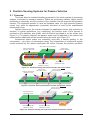
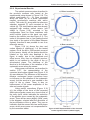
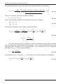
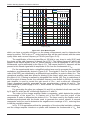
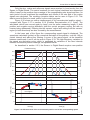
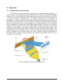
Figure 1.1 shows a simple example of combined transportation and processing of
materials with linear drives. In such applications, the following properties are necessary for
the linear drive system:
x The carriageway (track) must allow for horizontal and vertical curves, as well as for
closed paths and, possibly, switches (S).
x A number of processing stations (P1 … P3) are spread along the track.
x On the carriageway several vehicles (work-piece carriers, V1 … V4) must be able to
travel simultaneously, with a high degree of independency.
x Each vehicle has to be controlled very precisely (with an accuracy of a few
micrometers) when it operates within a processing station. This requires the use of
position sensors.
x While the vehicles are moving outside of the processing stations (i.e. in the
transport sections of the track), usually a lower precision in positioning is sufficient,
S =
S w it c h
V 1 . . . V 4 = V e h ic le s
( w o r k p ie c e c a r r ie r s )
C a r r ia g e w a y ( t r a c k )
P 1 ...P 3 =
P r o c e s s in g s t a t io n s
Figure 1.1: Simple example of combined transportation and processing of materials,
using a linear drives system
17
Introduction
so that a sensorless motion control should be used, avoiding the complexity and
costs introduced by position sensors.
The aim is to create a modular system, which allows for different properties at
different sections of the track:
x Straight sections
x Curved sections (left/right curves or up/downhill)
x Sections with high force for acceleration
x Sections for high precision positioning (equipped with position sensors), etc.
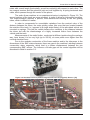
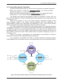
Two university departments cooperate in this project. The Institute for Electrical
Machines, Traction and Drives from Technische Universität Braunschweig is responsible
for the design of a new type of electrical machine (briefly presented in Section 3.1.1) and
all the mechanical constructions (track, vehicles). Our department is responsible for hardand software of power electronics and control of the proposed system.
Due to its high efficiency, high power density and because it allows a higher air gap,
the Permanent Magnet Synchronous Machine (PMSM) is a good choice for this
application. As high acceleration is mandatory, lightweight, passive vehicles, using an
active track, i.e. the long primary configuration of the PMSM (moving magnets), is the best
suited. With passive vehicles, there is no energy or information transfer from the stationary
side to the vehicle.
In order to allow for individual motion control of several vehicles, the active track is
separated into many segments [5], each segment being fed by the power stack of a
dedicated inverter. This approach has also the benefit of reduced losses, by turning off the
supply of the stator segments where there is momentarily no vehicle. Due to the modular
construction of the machine, there are gaps in the stator winding between consecutive
stator segments, which must be taken into consideration by the control algorithm.
As previously stated, position sensors are required within the processing stations.
Currently, there exists a multitude of linear position sensors, based on various physical
principles (optical, inductive, capacitive, Hall effect, magnetoresistive, magnetostrictive,
etc.) [6], [7]. However, not all of them are suitable for our application. The following requirements must be fulfilled by the position sensing system:
1. The vehicles are fully passive, i.e. there is no auxiliary energy source available on
board of the vehicles;
2. Measuring accuracy of a few micrometers;
3. Measuring length of several meters;
4. Measuring interval of 100 s or less;
5. The delay introduced in the position and speed control loops by the measuring
system has to be as low as possible, in order to allow for a high dynamic load
stiffness [8].
A detailed study [9], concerning different position sensing principles and commercially available position sensors was conducted at our department. Based on this study,
two types of position sensors, suitable for linear drives with passive vehicles, were
selected for evaluation: optical sensors and capacitive sensors.
In the transport sections of the linear drive for material handling described in this
work there are no requirements for high dynamics or high positioning precision. In these
sections, the complexity and costs introduced by position sensors will be avoided, by using
sensorless motion control.
There are several sensorless methods for PMSM that are found in literature. They
can be divided in two main classes:
18
Introduction
x Methods based on the evaluation of the Electromotive Force (EMF) or of the
mover’s flux [10], [11], [12]; these methods are relatively robust, but have the
disadvantage that they lose performance at low speed and do not work at standstill
(i.e. they can be used for sensorless travelling at speeds higher than a minimal
value, but they do not allow sensorless positioning).
x Methods based on the evaluation of the machine’s anisotropies [13], [14], [15],
usually by means of injecting a test signal. These methods are suited for standstill
and low speed range.
When compared to the rotating PMSM, the segmented, long primary, linear ones
present additional challenges with regard to the sensorless acquisition of the mechanical
quantities:
x The translator (vehicle) of a long primary linear machine covers only partially the
stator segments, which makes the extraction of the mechanical quantities from the
measurable electrical ones, more difficult.
x The mechanical quantities must also be acquired at the transitions between stator
segments.
All sensorless methods work incrementally, i.e. the absolute position cannot be
determined without the knowledge of an absolute, start position. In the particular case of
the discussed linear drives system, this start position can be determined when the vehicle
passes through a sensor-equipped section of the track.
A topology of the power electronics and the control system is proposed in [16] for a
similar linear drive. It consists on using two inverters, connected through static switches to
the different segments of the track. This configuration, however, allows driving only one
vehicle on the carriageway. Topologies that allow for multiple vehicles on the same track
are discussed in [5].
Methods to deal with the vehicle transition from one segment to other are
addressed in [17], [18] for the case of no gaps between segments. If there are gaps
between segments proposals can be found in [19], [20].
In the previous proposals, the position is assumed to be a known variable. The
usual approach for measuring the position is using a linear encoder with the read head in
the vehicle and a scale on the track. The position signal is then transmitted to the
stationary controller by a wireless modem, e.g. [18], [2]. This can be source of high delay
in the control loop, and low reliability. In addition, this arrangement needs an auxiliary
energy supply on board of the vehicle.
Using a magnetostrictive position sensor, as it is proposed in [4], the vehicle can be
totally passive. However, the position information has a large delay for longer distances,
which will not allow high dynamics in the control of movement (see also Section 2.1).
In this dissertation, a system and control method is proposed for a multi-segment
linear drive with totally passive vehicles, which allows for gaps between consecutive
segments, sensor based operation in some sections and sensorless based operation in
others. The main contributions are:
x A novel method for measuring the vehicle position with high accuracy and high
dynamics, using optical encoders, which method is suitable for use with passive
vehicles.
x Two new and improved evaluation methods for a commercially available capacitive
sensor that has a relatively lower resolution. This capacitive sensor could be used,
in certain applications, as a less complex, and more cost effective alternative to the
optical sensors.
x A method for handling the gaps and distinctive parameters among stator segments.
19
Introduction
x A procedure that allows the smooth handover (transition) of the vehicles between
the sensor-equipped, and the sensorless sections of the track.
This thesis is composed of two main sections: In Chapter 2, the two position sensing systems for passive vehicles, based on optical and capacitive sensors, respectively,
are presented, and their performance is evaluated. In Chapter 3, the position acquisition
and the control of the linear drive for material handling currently under development at our
department is discussed, including the overall system architecture, the sensor-based
position acquisition inside the processing stations, the sensorless position estimation in the
transport sections of the track, and the synchronisation between the position given by
sensors and the estimated one.
Finally, in Chapter 4, the conclusions are drawn, and future work, regarding the
expansion of the functionality of the linear drive for material handling presented in this
work, is outlined.
20
2 Position Sensing Systems for Passive Vehicles
2.1 Overview
The linear drive for material handling presented in this work consists of processing
stations, connected by transport sections. Within the processing stations, highly precise
positioning is necessary, thus the position of the vehicles must be acquired using position
sensors. The measured position is used as feedback value of a high precision position
control loop, while its approximate (numerical) derivative is used by the subordinated
speed control loop.
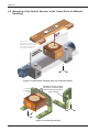
Optical sensors are the industry standard for applications where high precision is
required. In typical applications (e.g. machining), the passive scale of the sensors is
mounted on the stationary side (track), while the active read-head is on the vehicle (see
Figure 2.1). For passive vehicles, the passive scale must be attached to the vehicle and
several active read-heads will be mounted along the track, as in Figure 2.2.
Incremental optical scales are commonly used with a narrow grading, in the
micrometers – up to tens of micrometers range. Fine interpolation of sine/cosine signals
usually provided by the optical read-heads will further increase the position resolution
A c t iv e V e h ic le ( M o v in g W in d in g s )
P o w e r a n d I n f o r m a t io n
T r a n s f e r b y D r a g C h a in
P a s s iv e T r a c k
( S t a t io n a r y M a g n e t s )
M o v in g R e a d - H e a d
( A t t a c h e d t o V e h ic le )
S t a t io n a r y S c a le
(A tta c h e d to T ra c k )
Figure 2.1: Position sensing with optical encoder and active vehicle
S ta tio n a r y R e a d - H e a d s
(A tta c h e d to T ra c k )
M o v in g S c a le
( A tta c h e d to V e h ic le )
P a s s iv e V e h ic le
( M o v in g M a g n e ts )
A c t iv e T r a c k
( S t a t io n a r y W in d in g s )
Figure 2.2: Position sensing with optical encoder and passive vehicle
P a s s iv e V e h ic le
( M o v in g M a g n e ts )
A c t iv e T r a c k
( S t a t io n a r y W in d in g s )
R e c e iv in g E le c t r o d e
(A tta c h e d to T ra c k )
S ig n a l
P r o c e s s in g
T r a n s m it t in g E le c t r o d e
(A tta c h e d to T ra c k )
M o d u la t in g E le c t r o d e
( A t t a c h e d t o V e h ic le )
Figure 2.3: Position sensing with capacitive encoder and passive vehicle
21
Position Sensing Systems for Passive Vehicles
(nanometers range).
The capacitive sensor schematically depicted in Figure 2.3 is a low-cost, lowcomplexity alternative to the optical system from Figure 2.2. The passive slider, attached
to the vehicle, modulates (position-dependent) an electrical field produced between the
stationary transmitting and receiving electrode; the position can then be extracted by
demodulation.
Besides optical and capacitive sensors, there exist some more physical sensing
principles, which may be interesting for the discussed application, e.g. [21] where a sonic
strain pulse is induced in a specially designed magnetostrictive waveguide by the
momentary interaction of two magnetic fields. One field comes from a movable permanent
magnet fixed at the vehicle, as it passes along the outside of the sensor tube; the other
field comes from a current pulse (interrogation pulse) applied along the waveguide. The
interaction of the two magnetic fields produces a strain pulse, which travels at sonic speed
along the waveguide until it is detected at the head of the sensor. The position of the
magnet (= vehicle) is determined by measuring the elapsed time between the application
of the interrogation pulse and the arrival of the resulting strain pulse [22].
These sensors have many interesting properties such as absolute measurement,
possibility to simultaneously measure the position of several vehicles and to measure also
along curved tracks. But, due to the travelling time of the sonic stain pulse, the abovementioned requirements 4 and 5 are not fulfilled. The measuring cycle is 500 s for a
1,2 m measuring distance and 1000 s for 2,4 m [21], [23]. Therefore, these types of
sensors are interesting for other applications, where such a delay in the control loop can
be accepted.
The rest of this chapter is organised as follows:
In Section 2.2 a position sensing system for passive vehicles, based on optical
sensors (as shown in Figure 2.2) will be described. The hardware, firmware and software
developed for this position acquisition system will be presented, as well as experimental
results regarding the performance of the optical system.
Section 2.3 presents the evaluation of the capacitive sensor (Figure 2.3). Firstly, an
electrical model of the sensor will be derived. Then, two evaluation methods developed for
the capacitive sensor (based on rectangular and, respectively, on sinusoidal excitations)
will be presented. Experimental results for both excitation methods will also be shown and
compared.
22
Position Sensing Systems for Passive Vehicles
2.2 Optical Sensors System
2.2.1 General Description of the System
In this section, the implementation of an optical sensors system for use in linear
drives with passive vehicles will be described. Optical sensors are the industry standard
for position measuring when high precision positioning is required. The used sensor has
an incremental scale with a grading (pitch) of 40 μm, and in order to further increase the
resolution, the read-heads generate two analogue signals (sine and cosine) with a cycle
length equal to the pitch. Fine interpolation, using arctangent function, will provide a
position resolution (but not accuracy) in the nanometers range. The high resolution is
necessary in order to generate a smooth speed signal (for the speed control loop) as the
numeric derivative of position within a short sampling interval and without delay by filtering.
The sensors also provide a reference signal, used for the zero-position detection. For a
more detailed description of the sensors, see section 2.2.2.
Normally, the passive scale of the sensors has the same length as the maximal
travelling distance of the linear machine and is mounted on the stationary side, while the
active read-head is on the moving part. In the case of a passive mover, the mounting must
be reversed, which means that the length of the sensor’s scale is limited to the length of
the mover. If a travelling distance longer than the mobile part is required, more than one
read-head will be necessary.
In the proposed system, a number of five read-heads are spread along the
carriageway ca. 210 mm apart from each other, so that the 250 mm long scale covers at
any given position at least one read-head. Because it is not feasible to mount the heads at
distances that are exact multiples of the 40 μm pitch, one must calculate and compensate
for the difference between the phases of two neighbouring heads (as determined with the
arctangent function). When the scale passes from one read-head to the next one, the
signals from both heads will be simultaneously evaluated once, and the initial position of
the incoming read-head can be calculated. Future position calculations are based on this
initial value. Thus, a monotone variation of the calculated position along the entire
measuring length can be ensured.
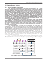
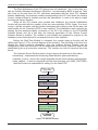
Figure 2.4 shows the block diagram of the proposed position acquisition system.
The signals from the read-heads are brought to a pre-processing unit (Sensor to Digital
S c a le
H
1
H
2
H
H
3
4
H
P o s it io n C a lc u la t io n
R o u t in e ( C C o d e )
5
P C I B u s
S ig n a l C o n d it io n in g
C o m p a ra to rs
A /D C o n v e rte rs
F P G A
R S -4 8 5 In te rfa c e
S e n s o r t o D ig it a l B o a r d
F P G A
P C I In te rfa c e B o a rd
M u lt ip le x e r s
P C I B u s B u ffe rs
O p t o c o u p le r s
R S -4 8 5 In te rfa c e
S e n s o r B u s
Figure 2.4: Block diagram of the optical position acquisition system
23
Position Sensing Systems for Passive Vehicles
Board). The analogue sine and cosine signals from two neighbouring heads are fed, via
multiplexers, into four analog-to-digital converters, where they are digitised, and sent
further to an Field Programmable Gate Array (FPGA). The FPGA calculates the coarse
position based on the sign bits of sine and cosine. It also keeps track of the current readhead and decides (based on the coarse position of the current read-head) when to start
evaluating the signals from the next read-head. The reference signals from the first and
last read-heads are also necessary, to detect when the vehicle enters the sensors covered
region. They are fed, through comparators, to the Sensor to Digital Board’s FPGA.
The pre-processing unit is connected through the Sensor Bus to a PCI Interface
Board. The Sensor Bus is a 16 bit parallel bus, implementing the RS-485 differential
signalling standard [24]. As its name suggests, the main purpose of PCI Interface Board is
to provide an interface between the Sensor Bus and the Peripheral Component
Interconnect (PCI) Bus [25] of a PC, where the control code (implemented in C language)
is running. The second role of the PCI Interface Board is to galvanically isolate the PC
from the rest of the position acquisition system, through optocouplers.
The position calculation routine is integrated in the control program and will be
called in every control cycle (100 μs). When a call occurs, it will send a request, via the
PCI Interface Board, to the pre-processing unit, which will send back the updated position
information. Based on this information, the routine calculates a new position value and
passes it to the control algorithm.
The detailed function of the component parts of the position acquisition system will
be presented in the following sections.
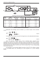
2.2.2 Sensors Used
For the proposed system, the linear optical encoder LIDA 181 [26] from Heidenhain
company (depicted in Figure 2.5) will be used. The encoder is based on imaging scanning
principle (for details, see Appendix 5.1) and has a grating period (pitch) of 40 μm. The
analogue sine and cosine signals (with a cycle length equal with the pitch) delivered by the
sensor are differential, in order to reduce the influence of noise and have a magnitude of
1 V peak-to-peak. It must be noted that in order to function as specified, the sensors
require a rather small gap between scale and read head (0.75 mm), with very small
tolerance (±150 μm) and also small angular tolerances. This can be quite challenging with
a linear machine where the guiding is not very stiff (see section 3.2). The most important
datasheet specifications of the used optical sensors are summarised in Table 2.1.
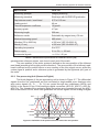
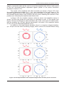
Figure 2.6 shows the definitions for the positive moving direction and for the zero
position. When the sensor moves in positive direction, the cosine signal has a phase of
+90° with respect to the sine (according to the trigonometric definition); when the sensor
moves in negative direction the cosine signal lags the sine (-90° phase). The periods are
counted based on the zero crossings of the sine when the cosine is positive: crossing from
4th to 1st quadrant increases the period counter, while crossing from 1st to 4th quadrant
decreases it. The reference pulses are centred in the middle of the 1st quadrant and can
have a width between 180° and 540°. This means there is exactly one period count (up or
down, depending on the moving direction) during a reference pulse. A read-head
Figure 2.5: LIDA 181 from Heidenhain. Source: [26]
24
Position Sensing Systems for Passive Vehicles
Specification
LIDA 181
Measuring principle
Imaging scanning
Measuring standard
Steel tape with AURODUR graduation
Gap between scale / read-head
0.75 ± 0.15 mm
Grating period
40 μm
Thermal expansion coefficient
10 ppm/K
Accuracy grade
± 5 μm
Measuring length
220 mm
Reference marks
Selectable by magnet every 50 mm
Maximal traversing speed
480 m/min
Vibration (55 to 2000 Hz)
200 m/s² (IEC 60 068-2-6)
Shock (11 ms)
500 m/s² (IEC 60 068-2-27)
Operating temperature
0 to 50°C
Power supply
5 V ± 5% / < 150 mA
Incremental signals
1 VPP / 40 μm
Table 2.1: Manufacturer specifications for LDIA 181. Source: [26]
generates two reference pulses, one close to each end of the scale.
The zero-position of the entire system is defined as the zero-position of the leftmost
read-head (assuming left-to-right positive direction). The zero-position of the leftmost readhead is defined as the position where a zero crossing of the sine signal occurs, whilst the
cosine signal is positive and a reference pulse is generated by the rightmost (sic!) part of
the scale.
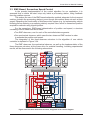
2.2.3 Pre-processing Unit (Sensor to Digital)
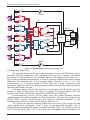
The block diagram of the pre-processing unit is shown in Figure 2.7. The differential
signals from the five read-heads are first converted to single-ended ones. Analogue sine
and cosine signals (S1, C1, … S5, C5) are routed through two multiplexers (MUXA and
MUXB) to the inputs of four 12-bit analog-to-digital converters (ADC-SA, ADC-CA, ADC-SB,
ADC-CB). The outputs of the analog-to-digital converters are connected through the ADCBus to the board’s FPGA, which also generates the control signals for the analog-to-digital
1 8 0 ° ± 9 0 °
1 8 0 ° ± 9 0 °
R e f.
C o s in e
S in e
Q u a d ra n t
P e r io d
1
2
3
-1
4
1
2
3
0
4
1
2
3
4
1
P o s it iv e d ir e c t io n
Figure 2.6: Definition of the positive direction and of the zero position
25
Position Sensing Systems for Passive Vehicles
R
C
S
M C
A
2 P
1
3
2 N
S
3 P
S
S
C
C
3
C
3 P
S
2
S B -W R
(1 6 b )
A
B
A D C -S
(1 2 b )
R S 4 8 5
D R V .
F P G A
(1 6 b )
B
R S 4 8 5
R C V .
B
4 P
4
S
4
4 N
C
C
B
5
C
4 P
M U X
S
4
A
A D C -C
A
3
3 N
S
A D C -S
A
5
3 N
C
3
A
A
2
S E N S O R -B U S
C
S
2
C
2 P
M U X
C
A D C -B U S
S
2 N
2
C
4
A D C -C
B
B
S B -R D
4 N
S
S
5 P
S
5 N
C
5
C
C
5 P
M C
5
5 P
B
5
C O M P -R
5 N
R
R
1
1 N
S
H
1
1
C
1 P
C
H
S
1 N
1
H
C O M P -R
1 P
S
H
1
1 N
S
H
R
1 P
R
R
5
5
5 N
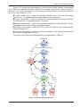
Figure 2.7: Block diagram of the pre-processing unit
converters and multiplexers.
The essential function of the signal processing that occurs in the FPGA is to ensure
that when the scale passes from one read-head to the next one no position information
loss occurs. To achieve this, the four analogue signals of the neighbouring heads (SA, CA,
SB, CB) will be sampled simultaneously, in order to correctly calculate their relative phase
difference. The sampling rate of the analog-to-digital converters is set to 2 μs. This
ensures that up to a maximal speed of 10 m/s there are at least 2 samples of the
sine/cosine signals in each 40 μm grating period of the sensor, and the position acquisition
algorithm can function correctly.
Reference signals from the first and from the last read-heads (R1 and R5) are also
needed, in order to detect when the vehicle is entering the sensors’ region. They are
brought to the FPGA, through two comparators (COMP-R1 and COMP-R5).
At the beginning of every 100 μs control cycle, the control algorithm requests
updated position information through the 16-bit Sensor Bus. This bus is connected to the
board’s FPGA through RS-485 drivers and receivers. Detailed description of the
communication protocol on Sensor Bus is given in section 2.2.4.
The vehicle can enter the sensors’ region from left or from right, so the sine and
cosine signals from read-heads 1 and 5 must be simultaneously available. This is
achieved when the signals from head 1 come through MUXA (MCA = 1), and the ones from
head 5, through MUXB (MCB = 5). On the other hand, the signals from read-head 4 are
26
Position Sensing Systems for Passive Vehicles
routed through MUXB, so when the vehicle is travelling in positive direction, at the
transition from head 4 to head 5, the sine and cosine signals of the last must be available
through MUXA (otherwise it would not be possible to sample the four signals
simultaneously). This is why S5 and C5 are routed through both MUXA and MUXB.
The distance covered by read-head 5 will be split in two: in the first half, the signals
from MUXA will be used, and in the second half, the signals from MUXB. So, to the physical
read-head 5 correspond two logical read-heads “5A” and “5B”, each covering half the
distance covered by head 5. At the transition between the two logical heads the position
phase difference is zero. In the following, heads 5A and 5B will be treated in the signal
processing as two different read-heads.
The realisation of the pre-processing unit (Sensor to Digital Board) is shown in
Figure 2.8. The five optical sensors are connected to the board through connectors
(1) … (5). In the signal conditioning part (6), the sensors signals are converted to singleended, their gain is adjusted, and the high frequency noise is filtered. The sine and cosine
signals are than routed, through the multiplexers (7) to the four analog-to-digital converters
(8), whilst the analogue reference signals from heads 1 and 5 are digitalized using the two
comparators (9). The threshold values of the comparators are adjustable, so that the
reference pulses can be kept in the limits defined by Figure 2.6.
The outputs of the comparators, as well as the ones from the analog-to-digital
converters are brought to the FPGA (10). EPROM (11) is used to store the FPGA firmware
when the power is off, and to automatically program the FPGA at power-up. The FPGA
can also be programmed using the connectors (13) or (14). An 80 MHz oscillator (12)
generates the clock signal. Auxiliary input/output port (15) can be used for debugging. In
the area (16) are the RS-485 drivers and receivers for the Sensor Bus, and (17) is the
connector for the Sensor Bus cable.
The board requires +5 V and –5 V power supplies for the analogue circuitry, and a
separate 5 V supply for the digital one. These are supplied to the board using the
connector (18). Additionally, the FPGA also needs 3.3 V and 1.5 V supplies, which are
1
2
3
4
5
6
7
7
9
9
8
8
1 5
1 2
8
1 3
1 0
1 1
1 4
1 9
1 6
1 8
8
1 7
Figure 2.8: Realisation of the preprocessing unit (Sensor to Digital Board)
27
Position Sensing Systems for Passive Vehicles
generated on the board, using the DC/DC converters (19).
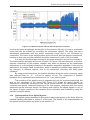
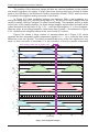
The distances covered by each read-head are shown in Figure 2.9. The scale has a
length of 250 mm, and the read-heads are mounted along the track at approximately every
210 mm. Considering the grating period (Pitch) P = 40 μm of the sensor, each of the
heads 1 … 4 will cover a number N = 5250 periods. Head 5A covers N/2 = 2625
periods, whilst head 5B covers N5B periods. If the heads would be mounted exactly N
periods apart from each other, the relation N5B = N/2 would hold true, but in reality a
small difference exists (on the experimental setup a difference of 5 periods was identified).
N5B can be determined during a test-run in the positive direction, as the value of the “B”
period counter on the falling edge of the second pulse of the reference signal R5 (see
below). If instead of the real value N5B, the ideal value N/2 is used, a hysteresis of the
determined position occurs between runs in positive and negative directions.
R
R
1
D N
H
D N
1
H
D N
2
H
D N
3
H
5
D N /2
4
H
Z e r o P o s it io n
5 A
D N
H
5 B
5 B
M a x im a l P o s it io n
Figure 2.9: Distances between read-heads
The values N, N/2, and N5B will be used by the FPGA to decide when the
transition between one read-head and the following one must be made.
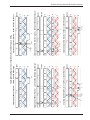
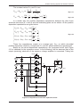
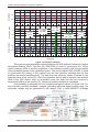
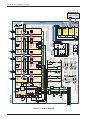
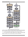
The firmware in the Sensor to Digital FPGA (a simplified diagram of which is shown
in Figure 2.10) can be divided in seven major functional blocks:
1. ADC Control – controls the four analog-to-digital converters.
2. Sin/Cos Registers – store the conversions’ results.
3. Counter A Control – controls a 14-bit counter (CNTRA) which counts the periods
(coarse position) of the read-head currently routed through MUXA, based on the
sign bits of SA and CA.
4. Counter B Control – identical with Counter A Control, CNTRB counts based on the
sign bits of SB and CB.
5. Current Head Control – controls the Current Head State Machine (CHSM), which
keeps track of the read-head(s), currently covered by the scale. Additionally, this
block generates the control signals for the two multiplexers (MCA and MCB).
6. Sensor Bus Control – implements the interface with the Sensor Bus
7. Synchronisation – generates the timing and the synchronisation signals for all
previous blocks.
It is assumed that initially the vehicle is outside the sensors’ region. The Current
Head State Machine is in state H0 (signifying that no read-head is covered by the scale).
The CHSM uses two 3-bit buses, LDA(3) and LDB(3) to control the behaviour of the two
period counters CNTRA(14) and CNTRB(14). The possible values for LDA and their
meaning are given in Table 2.2. Those of LDB are similar, with the only difference that for
LDB = 100b the value N5B instead of N/2 is loaded in CNTRB. In the initial state,
LDA = 001b and LDB = 100b, meaning that the two counters will be blocked, holding the
values NA = -1 and NB = N5B, respectively.
Multiplexer code register R-MCA(2) holds the value MCA = 1, so that SA = S1,
CA = C1, and R-MCB(2) – the value MCB = 5 (SB = S5, CB = C5). Registers R-USEA and RUSEB indicate whether position information from heads “A” or “B”, respectively, is valid and
should be used for position calculation. Initially they are both reset – neither of the active
heads (1 and 5B) is providing valid signals. The Conversion Timer (in the Synchronisation
28
Position Sensing Systems for Passive Vehicles
A D C C O N T R O L
R -C A(1 2 )
R -T M P -S B(1 2 )
R -S B(1 2 )
R -T M P -C B(1 2 )
R -C B(1 2 )
A
R B -S B(1 2 )
C B(1 2 )
T O A
R E G IS T
A N D S T
M A C H I
R B -C B(1 2 )
B
B
B
S
-1
D N
B
C
N
C N T R A(1 4 )
C U P
B
U P D T A T E -S C -R E G
A D C -S T A R T
A D C -F IN IS H E D
M S B (C A)
M S B (S B)
M S B (C B)
C D N
A
Q U A D R A N T B
S T A T E M A C H IN E
C D N
B
S E L E C T
C N T R B(1 4 )
S Y N C H R O N IS A T IO N
S T A T E M A C H IN E
R B -N
(1 4 )
A
R -M C A(2 )
R B -M C A(2 )
R -M C B(2 )
R B -M C B(2 )
R -U S E
R -U S E
R 1'
B
-1
D N
(1 4 )
S B -O U T
(1 6 )
A
Q U A D R A N T A
S T A T E M A C H IN E
C U P
A
C U R R E N T
H E A D C O N T R O L
D N /2
B
C O N V E R S IO N
T IM E R (2 µ s )
B
(3 )
A
N
L D
U S E
U S E
B
(3 )
B
B
R 5'
R B -U S E
A
R B -U S E
B
S B -A C K
R B -N
(1 4 )
B
A
A
R
R
1
5
1
(1 4 )
R B -R
5
B
R B -R
S B -W R
S B -R D
C O U N T E R B C O N T R O L
D N
5 B
(1 4 )
E N A
R -D N
5 B
(1 4 )
S E L E C T
R -E N A
S B -A C K
S B -R E Q
R S -4 8 5 D R IV E R S
S
S
S
M C B(2 )
M U X
L D
L L
E R S
A T E
N E S
S B -IN
(1 6 )
R S -4 8 5 R E C E IV E R S
A
M S B (S B -IN )
A
S E N S O R B U S C O N T R O L
S T A T E M A C H IN E
C
A
C O U N T E R A C O N T R O L
S E L E C T
A
F P G A
R E S E T
M C A(2 )
M U X
A
C
F P G A
C L O C K
R B -C A(1 2 )
S B(1 2 )
S B -A C K
A
C
C
R B -S A(1 2 )
C A(1 2 )
U P D T A T E -S C -R E G
S
S
M S B (S A)
S Y N C H R O N IS A T IO N
S E N S O R -B U S -C O N T R O L
S A(1 2 )
S B -R E Q
S
R -T M P -C A(1 2 )
S E L E C T
S S D S S D S S D S S D -
R -S A(1 2 )
A D C C O N T R O L
S T A T E M A C H IN E
/C
/B
/R
/C
/B
/R
/C
/B
/R
/C
/B
/R
S IN /C O S R E G IS T E R S
R -T M P -S A(1 2 )
C U R R E N T H E A D
S T A T E M A C H IN E
A D C -C
B
A D C -S
B
A D C -C
A
A D C -S
A
A D C -B U S (1 2 )
R 1'
C O M P -R
C O M P -R
5
1
R 5'
R
R
1
5
Figure 2.10: Simplified diagram of the pre-processing unit FPGA code
Block) is stopped, and no analog-to-digital conversions take place. The system remains in
this state until one of the comparators’ outputs (R1 or R5) is asserted, signalling the
entering of the vehicle into the sensors’ region (from left or from right).
Let us assume that the vehicle comes from left, thus travelling in the positive
direction. The synchronisation logic detects the rising edge of R1 and asserts the signal
ADC-START and simultaneously starts the 2 μs Conversion Timer. It then waits for the
first conversion to end.
When the ADC-START signal is asserted, the ADC Control State Machine
immediately asserts the four conversion start signals (/CS-SA, /CS-CA, /CS-SB, /CS-CB).
The conversions are finished after a maximum time of 750 ns [27], which is indicated by
LDA(3)
000b
001b
010b
100b
Other
Signification
CNTRA is enabled and counts based on MSB(SA) and MSB(CA)
Value –1 is loaded in register CNTRA
Changes in MSB(SA) and
MSB(CA) have no influence
Value N is loaded in register CNTRA
Value N/2 is loaded in register CNTRA on the counter’s value
Illegal
Table 2.2: Possible values of LDA
29
Position Sensing Systems for Passive Vehicles
the de-asserting of the four busy signals (/BS-SA, … /BS-CB). At this point, the four read
signals (/RD-SA, … /RD-CB) are used to sequentially bring the conversions’ results into
four temporary registers R-TMP-SA(12), … R-TMP-CB(12). This sequential reading through
the ADC-BUS(12) takes 200 ns. After that, the ADC Control State Machine asserts the
ADC-FINISHED signal, determining the Synchronisation State Machine to assert the
UPDATE-SC-REG signal, thus simultaneously updating the content of registers R-SA(12),
R-CA(12), R-SB(12), and R-CB(12).
Based on the new values of SA and CA (their sign bits) the Quadrant A State
Machine will be set in the correct state. The first conversion was made soon after the rising
edge of R1. This means that the quadrant determined by SA and CA can be 2, 3 or 4,
depending on the width of R1 (see Figure 2.6). As previously stated, CNTRA is blocked at
the value –1 by CHSM. Because the scale does not cover head 5B, the values of SB and
CB are at this point irrelevant.
Two clocks after the UPDATE-SC-REG signal was asserted (leaving time for the
sine/cosine registers and for quadrant state machines to stabilize), the synchronization
state machine asserts R1’, leading to the transition of the CHSM from state H0 into state
H1A(1). The complete Current Head State Machine is shown in Figure 2.11. In state H1A(1),
LDA = 000b, thus CNTRA is enabled and the value “1” is stored in R-USEA, indicating valid
position information from head “A” (in this case 1). The multiplexers’ control signals remain
unchanged.
At this point the content of all the position information registers (sine/cosine
registers, period counters, multiplexer code registers and “use” registers) is consistent,
indicating the new state of the system: the vehicle is at the beginning of the region covered
by of head 1, and its position can be correctly calculated based on the “A” values. The “B”
position information will be ignored until the scale covers a read-head whose signals are
routed through the “B” multiplexer.
The reference signal R1 (or R5, if entering from right) is used only to trigger the first
conversion cycle and, when this first conversion is finished, the first transition in CHSM. All
the subsequent reference pulses are ignored, until the vehicle is again outside the
sensors’ region.
When the conversion timer (started at the same time with the first conversion) hits
2 μs a new conversion is started and, after it is finished, new values of SA, CA, SB, and CB
will be available, leading to the update of the quadrant state machines and of the period
counters and, based on the updated counters’ values to the update of the state of CHSM.
During this update time, the position information can be inconsistent. The redundant
temporary sine/cosine registers in the ADC Control block where introduced to minimize
this inconsistency time. Instead of 200 ns (as it takes to sequentially update the four
conversion results through the ADC Bus), the time for updating of the sine/cosine registers
(R-SA, … R-CB) is reduced to one FPGA clock (12.5 ns). Adding to this time the time
necessary to update the quadrant state machines, the period counters, and the CHSM, an
inconsistency time of 50 ns results. Any data request coming from Sensor Bus during this
time will be delayed until the position information registers are consistent again, and the
delay must be short enough not to impair the timing requirements of the Sensor Bus
protocol.
When the Sensor Bus Control State Machine receives a position information
request, it asserts the SB-REQ signal. The Synchronisation State Machine responds by
asserting the acknowledge signal SB-ACK, with a delay no longer than 50 ns, if necessary,
as discussed above.
30
Position Sensing Systems for Passive Vehicles
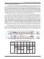
H
V e h ic le o u t s id e s e n s o r
r e g io n ( in it ia l s t a t e )
H
R e s e t
N
H
N
S c a le c o v e r s
h e a d 1 ( s e c o n d h a lf )
N
H
H
S B -A C K
1 A -2 B
N
H
N
N
N
N
H
2 B -3 A
N
H
N
H
N
S c a le c o v e r s
h e a d 3 ( s e c o n d h a lf )
N
H
H
N
H
> = -1
B
N
H
N
S c a le c o v e r s
h e a d 4 ( s e c o n d h a lf )
N
N
H
4 B -5 A
N
N
N
S y n c h r o n is a t io n
b e tw e e n h e a d s 5 A a n d 5 B
N
H
5 A -5 B
A
B
R e s e t
U S E A= 0
L D A= 0 0 1
(N A= -1 )
U S E B= 1
L D B= 0 0 0
(N B c h a n g e s )
4
5
U S E A= 1
L D A= 0 0 0
(N A c h a n g e s )
U S E B= 1
L D B= 0 0 0
(N B c h a n g e s )
4
5
U S E A= 1
L D A= 0 0 0
(N A c h a n g e s )
U S E B= 0
L D B= 0 1 0
(N B= D N )
4
5
U S E A= 1
L D A= 0 0 0
(N A c h a n g e s )
U S E B= 0
L D B= 0 0 1
(N B= -1 )
5
U S E A= 1
L D A= 0 0 0
(N A c h a n g e s )
U S E B= 1
L D B= 0 0 0
(N B c h a n g e s )
5
U S E A= 0
L D A= 0 1 0
(N A= D N )
U S E B= 1
L D B= 0 0 0
(N B c h a n g e s )
5
U S E A= 0
L D A= 0 0 1
(N A= -1 )
U S E B= 1
L D B= 0 0 0
(N B c h a n g e s )
U S E A= 1
L D A= 0 0 0
(N A c h a n g e s )
U S E B= 1
L D B= 0 0 0
(N B c h a n g e s )
U S E A= 1
L D A= 0 0 0
(N A c h a n g e s )
U S E B= 0
L D B= 0 1 0
(N B= D N )
U S E A= 1
L D A= 0 0 0
(N A c h a n g e s )
U S E B= 0
L D B= 0 0 1
(N B= -1 )
U S E A= 1
L D A= 0 0 0
(N A c h a n g e s )
U S E B= 1
L D B= 0 0 0
(N B c h a n g e s )
U S E A= 0
L D A= 1 0 0
(N A= D N /2 )
U S E B= 1
L D B= 0 0 0
(N B c h a n g e s )
U S E A= 0
L D A= 0 0 1
(N A= -1 )
U S E B= 1
L D B= 0 0 0
(N B c h a n g e s )
U S E A= 0
L D A= 0 0 1
(N A= -1 )
U S E B= 0
L D B= 1 0 0
(N B= D N 5B)
3
A
3 A (2 )
3
A
2
1
2
B
B
0
4 B (1 )
3
H
4
B
4 B (2 )
3
1
2
3
1
2
3
4
B
4 B -5 A
H
B
3
1
2
3
4
1
2
3
4
1
2
3
4
A
3
5
A
5 A (2 )
4
5 A
5
A /B
-5 B / H
5 B -5 A
5
A /B
H 5B
-1
5
A /B
H 5
< = D N /4
2
5
5 A (1 )
H
2
1
5 A -4 B
A
4
1
A
A
/H
4
B
< -1
R 5 '= 1
H
B
H
A
4
H
5 B (2 )
5 B
4 B -3 A
3
H
5 B (1 )
N
B
/H
3 A -4 B
A
1
5 B -5 A
N
H
> D N
5
< -1
A
H
> = -1
> D N /4
B
4
> = D N /2
N
S c a le c o v e r s
h e a d 5 (fo u rth q u a rte r)
N
3
3 A (1 )
H
5 A (2 )
H
B
U S E B= 1
L D B= 0 0 0
(N B c h a n g e s )
< = D N /4
A
S B -A C K
N
U S E A= 0
L D A= 0 1 0
(N A= D N )
S B -A C K
N
H
2
5 A -4 B
N
> D N /2
A
1
5 A (1 )
> D N /4
A
5
< -1
B
H
> = -1
A
H
S c a le c o v e r s
h e a d 5 (s e c o n d q u a rte r)
4
> = D N
B
S B -A C K
S c a le c o v e r s
h e a d 5 ( f ir s t q u a r t e r )
3
S B -A C K
N
H
U S E B= 1
L D B= 0 0 0
(N B c h a n g e s )
3 A -2 B
S
2
4 B (2 )
> D N
B
S y n c h r o n is a t io n
b e tw e e n h e a d s 4 a n d 5
U S E A= 1
L D A= 0 0 0
(N A c h a n g e s )
A
H
< = D N /2
B
5
3
2
1
4 B (1 )
> D N /2
B
4
A
/H
2
B
4 B -3 A
S B -A C K
S c a le c o v e r s
h e a d 4 ( f ir s t h a lf )
B
2 B -3 A
S B -A C K
3 A -4 B
3
2 B (2 )
2
> = D N
A
U S E B= 0
L D B= 0 0 1
(N B= -1 )
2
B
B
< = D N /2
A
U S E A= 1
L D A= 0 0 0
(N A c h a n g e s )
2
1
3 A (2 )
N
S y n c h r o n is a t io n
b e tw e e n h e a d s 3 a n d 4
H
1
N
> D N
A
H
3 A (1 )
> D N /2
A
5
3
< -1
A
4
2
B
2 B (1 )
1
A
3 A -2 B
> = -1
A
U S E B= 0
L D B= 1 0 0
(N B= D N 5B)
4
B
H
1
S B -A C K
S c a le c o v e r s
h e a d 3 ( f ir s t h a lf )
A
> = D N
B
U S E A= 1
L D A= 0 0 0
(N A c h a n g e s )
3
B
2 B -1 A
1
< = D N /2
B
5
2
B
/H
1 A -2 B
S B -A C K
N
H
H
2 B (2 )
> D N
B
S y n c h r o n is a t io n
b e tw e e n h e a d s 2 a n d 3
1
A
< -1
B
U S E B= 0
L D B= 1 0 0
(N B= D N 5B)
4
1 A (2 )
2 B (1 )
> D N /2
B
A
H
2 B -1 A
> = -1
B
H
S c a le c o v e r s
h e a d 2 ( s e c o n d h a lf )
V e h ic le o u t s id e s e n s o r
r e g io n ( in it ia l s t a t e )
> = D N
U S E A= 0
L D A= 0 0 1
(N A= -1 )
3
1
1 A (2 )
A
5
2
1 A (1 )
< = D N /2
A
S B -A C K
S c a le c o v e r s
h e a d 2 ( f ir s t h a lf )
S c a le c o v e r s
h e a d 5 ( t h ir d q u a r t e r )
N
N
S y n c h r o n is a t io n
b e tw e e n h e a d s 1 a n d 2
H
A
1 A (1 )
> D N
A
< -1
A
> D N /2
A
1
0
R 1 '= 1
S c a le c o v e r s
h e a d 1 ( f ir s t h a lf )
0
B
4
B (2 )
5
B
H
0
5
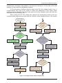
Figure 2.11: Current Head State Machine (CHSM)
31
Position Sensing Systems for Passive Vehicles
On the rising edge of SB-ACK, the content of the position information registers is
transferred into a set of corresponding bus registers:
x Sine/cosine registers
RB-SA(12), RB-CA(12), RB-SB(12), RB-CB(12);
x Period counters
RB-NA(14), RB-NB(14);
x Multiplexers’ codes
RB-MCA(2), RB-MCB(2);
x Used (valid) head
RB-USEA, RB-USEB;
x Reference signals
RB-R1, RB-R5.
From these registers the position information will be sent further on the Sensor Bus.
The position information is updated in the Sensor to Digital FPGA every 2 μs. The content
of the bus registers listed above is a consistent snapshot of this information, taken every
100 μs, when it is required by the control.
The data stored in registers R-ENA and R-N5B(14) is coming from the control
program. Register R-N5B(14) contains the real number of periods covered by head 5B (as
determined during a test-run). Its contents will be written only once, when the control
program starts. A zero written in R-ENA will determine the Synchronisation State Machine
to ignore the reference signals, thus effectively disabling all the position acquisition related
firmware in the Sensor to Digital FPGA. This behaviour is useful for the initialisation phase,
when the control must ensure that the vehicle is outside sensors’ region before enabling
the Sensor to Digital algorithm.
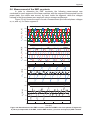
State H0 corresponds in the CHSM to the vehicle being outside sensor’s region. For
each of the six logical read-heads (1 … 4, 5A, 5B) there are two states. The only
difference between the two states is in the multiplexers’ control signals. For example, in
state H1A(1), the signals from head 1, coming through MUXA, are used to determine the
position. In this state MCB = 5. When the middle of the scale passes the head (NA > N/2),
a transition to state H1A(2) occurs, where MCB = 2. CNTRB continues to remain blocked, but
LDB changes to 001b, so the value –1 will be now loaded into the counter. Thus, the
signals from head 2 are now coming through MUXB to the analog-to-digital converters and
are ready for evaluation. The multiplexers’ codes corresponding to each state of CHSM
are depicted on the diagrams on the right of the state machine in Figure 2.11. The values
of USEA, USEB, LDA and LDB are also listed for each state.
When in state H1A(2) and NA > N, there is no direct transition to state H2B(1).
Because the control program must determine the offset of head 2, the position information
of both heads, from the same 2 μs sample, must be sent through the Sensor Bus. So,
when NA > N, the transition to state H1A-2B occurs. In this state LDB is set to 000b (so
CNTRB is also enabled), and the position information from both heads is now valid
(indicated by USEA and USEB being both set). This state is maintained until after a read
request from the Sensor Bus is acknowledged, i.e. until the falling edge of SB-ACK comes.
When this happens, the CHSM goes into state H2B(1), where only the “B” position
information will be used. The transition between H2B(1) and H1A(2) (vehicle travelling in the
negative direction) happens similarly, passing in this case through state H2B-1A.
Some examples of transitions of the CHSM states will be illustrated in the last part
of this section, based on the CHSM representation in Figure 2.11, and on the simplified
signal diagrams in Figure 2.12:
a) Entering sensor’s region, moving in positive direction
Initially, CHSM is in state H0 and CNTRA is blocked to –1. When the rising edge of
R1 comes (time t1), the sampling of SA = S1 and CA = C1 begins. At time t2 (when the first
conversion is finished), CHSM changes state to H1A(1) and CNTRA is enabled. At time t3
(after passing through the zero position of the sensors’ region) CNTRA counts up, yielding
NA = 0, and continues counting based on the sign bits of SA and CA.
32
Position Sensing Systems for Passive Vehicles
N
C
C
C
R
S
S
S
A
A
A
A
A
A
B
B
B
1
D N -1
H
H
-1
0
1 A (2 )
-1
D N
t1 t2 t
t
3
1
0
D N + 1
t
2
0
1
H
1 A (1 )
1 A -2 B
D N + 2
H
1
2
D N + 4
D N + 3
t
3
2
t
4
3
H
3
2 B (1 )
D N
a) Entering sensors’ region – moving in positive direction
C H S M
N
N
S B -A C K
C H S M
C
R
S
B
B
B
5
D N
5 B
-3
D N
5 B
-2
H
D N
5 B
t
1
-1
D N
5 B
t2t3t
4
D N
5 B
D N
H
0
5 B
+ 1
b) Transition between heads 1 and 2 – moving in positive direction
N
C H S M
5 B (2 )
N
C
C
C
R
S
S
S
A
A
A
A
A
A
B
B
B
1
1
2
H
0
1
D N
2 B (1 )
H
1 A (1 )
-1
t
1
0
t
1
t
t
2
2
-2
-1
D N -1
H
t3t4t
2 B -1 A
-3
5
D N -2
-2
H
-1
-4
t
0
3
4
H
1 A (2 )
-1
D N -3
t
f) Leaving sensors’ region – moving in negative direction
C H S M
N
N
S B -A C K
C H S M
C
R
S
B
B
B
5
H
0
D N
5 B
t1 t
2
D N
5 B
-1
D N
H
5 B
5 B (2 )
-2
D N
5 B
-3
D N
5 B
-4
e) Transition between heads 2 and 1 – moving in negative direction
N
C H S M
d) Entering sensors’ region – moving in negative direction
Figure 2.12: Examples of state transitions in Current Head State Machine
c) Leaving sensors’ region – moving in positive direction
33
Position Sensing Systems for Passive Vehicles
Any reading of the position information before t2 will result in USEA = 0 and
USEB = 0 (vehicle outside sensor’s region). If the position information is read between t2
and t3, the control program will calculate a negative value of the position.
b) Transition between heads H1 and H2, moving in positive direction
The vehicle is travelling the region covered by head 1. When it approaches the end
of this region, the scale will also cover head 2. CHSM is in state H1A(2), and CNTRA is
counting. The sine/cosine signals from head 2 are coming through MUXB, but CNTRB is
blocked at –1 (not counting). When NA > N (at time t1), CHSM switches to state H1A-2B
and CNTRB is enabled. At time t2, the quadrant defined by SB and CB changes from 4 to 1
and CNTRB counts up, yielding NB = 0. The two counters are now both counting in parallel,
until t3, when the rising edge of SB-ACK arrives. The position information is saved into the
bus registers, and on the falling edge of SB-ACK (time t4) CHSM changes state to H2B(1).
CNTRB continues counting, but CNTRA is blocked, holding NA = N. State H1A-2B can last
up to 100 μs (the interval between two successive readings on the Sensor Bus), which
translates in up to 25 position periods (1 mm) at the maximum speed of 10 m/s.
c) Leaving sensors’ region, moving in positive direction
The scale covers head 5B, CHSM is in state H5B(2) and CNTRB is counting. At time
t1 the reference signal R5 comes, but this has no influence on the Synchronisation block.
The position acquisition algorithm in the Sensor to Digital FPGA will ensure that the
transition to state H0 will occur after the falling edge of R5 based solely on the value of
CNTRB. If the reference signal respects the tolerances defined in Figure 2.6, the falling
edge of R5 will come at the latest in the middle of quadrant 4 of period N5B, so the state
transition in CHSM will be triggered by NB > N5B. At time t3, CNTRB counts up and NB
becomes N5B+1. One FPGA clock later (time t4) CHSM switches to state H0, setting
LDB = 100b and another clock later (time t5) CNTRB is blocked, outputting NB = N5B.
d) Entering sensor’s region, moving in negative direction
The vehicle is outside of the sensors’ region, moving in negative direction, and
approaching read-head 5 from the right (i.e. logical head 5B). CHSM is in state H0. At time
t1 the rising edge of R5 comes and all four sine/cosine signals are sampled. In this case
SB = S5 and CB = C5 are relevant. After first conversion, CHSM changes to state H5B(2), at
time t2. CNTRB is enabled (before it was blocked to N5B) and position information “B” is
now valid.
e) Transition between heads H2 and H1, moving in negative direction
The scale covers heads 2 and 1, with the vehicle moving in negative direction.
CHSM is in state H2B(1), CNTRB is counting down, and CNTRA is blocked at NA = N.
When NB < –1 (time t1), the transition to state H2B-1A occurs and CNTRA is enabled
(LDA = 000b). At t2 quadrant A changes from 1 to 4, and CNTRA counts down (NA = N–1).
The two counters run in parallel and the position information from both heads is ready for
evaluation until t3, when, on the rising edge of SB-ACK, it is copied to the bus registers. On
the falling edge of SB-ACK (t4) the transition to H1A(2) occurs, CNTRB is disabled and
loaded with NB = –1, the “B” position information is invalidated (USEB = 0), and the position
evaluation will continue based only on the “A” values.
f) Leaving sensors’ region, moving in negative direction
The vehicle is close to the left limit of the region covered by head 1, moving in
negative direction. CHSM is in state H1A(1) and CNTRA counts down. At t1 the rising edge
of R1 occurs, but it has no effect. At time t2 the zero position of the sensors system is
crossed towards negative values. At t1, NA becomes less than –1, so at t4 (one FPGA clock
later) CHSM changes state to H0, and another clock later –1 is stored in CNTRA. The
system is now again in its initial state, waiting for one of the two reference signals.
34
Position Sensing Systems for Passive Vehicles
2.2.4 Sensor Bus Communication
The Sensor Bus connects the Sensor to Digital Board with the PCI Interface Board.
It is a 16-bit parallel bus, implementing the RS-485 differential signalling standard. Line 15
(the most significant bit) of the bus is used as control signal, whilst the other 15 lines
(14 … 0) are used as data lines. So, in one transfer (frame) 15 information bits can be sent
simultaneously through the bus. At one given time, one of the two communication parties
drives all the lines of the bus (control and data). This signalling technique was adopted
because it allows for a frame length that is not dependent on the delays on the bus (delays
caused by the RS-485 drivers and receivers, the propagation delay on the bus cable, and
especially delays caused by the optocouplers on the PCI Interface Board).
Figure 2.13 shows the transfer protocol between the Sensor to Digital and the PCI
Interface Board. In the upper part of the figure the control and data signals are sketched as
“seen” from the PCI Interface FPGA, while in the lower part as “seen” from Sensor to
Digital FPGA. Initially, the PCI Interface drives the bus, holding all the lines at logical 1.
When required from the control program (time t0) it starts sending a data request to the
Sensor to Digital Board. Data frame D0 (sent from control program) accompanies this data
request. The content of D0 is listed in Table 2.3: bit 14 (ENA) will be saved in the R-ENA
register of the Sensor to Digital FPGA and will enable or disable the position acquisition
algorithm. Bits 13 … 0 contain the real number of periods covered by head 5B. The sign
bit of N5B is not sent on the bus (it is always 0), but instead the SET5B bit will be sent.
This bit is used to save N5B in R-N5B only once, at the beginning of the control program.
Frame D0 is held on the bus until t3 (400 ns). In this time the control line is held low
for 200 ns and then back high for the remaining 200 ns. This line is acting as bus clock
signal: on its falling edges the communication party driving the bus lines writes data on the
bus, whilst on its rising edges the other party reads the data. The low and high pulses of
S e n s o r t o D ig it a l
P C I In te rfa c e
t
t
0
t
3
t
6
t
7
T
t
9
T
t
1 0
t
1 1
t
1 2
t
1 3
t
1 5
1 6
t
t
1 7
1 8
1 5
1 4 ..0
7 F F F
D 0
H
T
Z
D 1
T
D
T
Z
D 2
D 3
T
D
T
P
D 4
D 5
D 6
Z
7 F F F
T
P
D 0
H
Z
1 5
1 4 ..0
7 F F F
D 0
H
t
1
t
2
t
Z
4
D 1
t
D 2
t
5
D 3
D 4
D 5
D 6
Z
t
8
7 F F F
H
D 0
1 4
Figure 2.13: Sensor Bus transfer protocol
Frame
D0
D1
D2
D3
D4
D5
D6
14
ENA
USEA
0
0
USEB
0
0
13
SET5B
R1
MCA
(2)
R5
0
0
MCB
(2)
SA
(12)
CA
(12)
SB
(12)
CB
(12)
Bit
12
11
···
N5B
(13)
NA
(14)
NB
(14)
0
Table 2.3: Sensor Bus data frames
35
Position Sensing Systems for Passive Vehicles
the control line are 200 ns (TP) long, each.
After the time t3, the PCI Interface stops driving all the bus lines, setting the bus
drivers in high impedance state (Z). The Sensor to Digital FPGA detects the falling edge of
the control signal at time t1, after the delay time TD. Measurements have determined that
on the experimental setup this delay does not exceed 130 ns. The bus delay has no
influence on the pulse period TP, but must be known, for the Sensor Bus protocol to
function correctly. The data will be saved in the Sensor to Digital FPGA registers at time t2,
on the rising edge of the control signal. Simultaneously, a data request is signalled, by
asserting the SB-REQ signal. Between t4 and t5 the bus lines are not driven by any of the
two parties. The high impedance state lasts for TZ = 200 ns. Between t2 and t5 the data
request must be acknowledged (by the Synchronisation block in the Sensor to Digital
FPGA), and the position information saved in the bus registers. The contents of the bus
registers will be sent on the Sensor Bus in six data frames D1 … D6, which are also listed
in Table 2.3.
At time t6, after another delay period TD, data frame D1 will be “seen” by the PCI
Interface FPGA and it will be saved at time t7. The remaining data frames will also be sent
and saved in the PCI Interface FPGA registers at t9, t10, … t13. At t14, the Sensor to Digital
has sent all the position information and stops driving the bus lines. After receiving the last
data frame (t15), the PCI Interface does not immediately start to drive the bus; a second
high impedance state occurs between t15 and t16 and afterwards the PCI Interface drives
all the bus lines at logic 1.
It is possible to initiate a new transfer as soon as t17. The total transfer time on the
Sensor Bus amounts to TT = 2·TP·(1+6) + 2·TZ + 2·TD, which is about 3.5 μs. The bus will
remain in the idle state (all lines driven to “1” by PCI Interface) until a new position request
comes from the control program (the time interval t0 … t18 in Figure 2.13 is the 100 μs
control cycle).
2.2.5 PCI Interface Board
The PCI Interface Board assures the data transfer between the Sensor Bus and the
PCI Bus of the control PC. It does not alter in any way the position requests from control
program, nor the position information sent by the Sensor to Digital Board, acting solely as
a data transfer relay. It also provides galvanic separation between the control PC and the
position acquisition electronics on the Sensor to Digital Board. The realisation of the board
is shown in Figure 2.14:
(1) PCI Interface FPGA;
(2) EPROM, storing the FPGA firmware;
(3) 80 MHz oscillator;
(4) PCI Bus buffers;
(5) PCI connector;
(6) JTAG programming connector;
(7) Active Serial programming connector;
(8) Auxiliary inputs/outputs, used for debugging;
(9) 5 V and 3.3 V power supplies, connected to those coming through PCI connector;
(10) DC/DC converter, for the 1.5 V supply required by the FPGA;
(11) Optocouplers, separating the potentials of PC and Sensor to Digital Board;
(12) Sensor Bus drivers and receivers;
(13) Sensor Bus connector;
(14) Separate 5 V supply for the Sensor Bus drivers and receivers.
36
Position Sensing Systems for Passive Vehicles
1 1
6
1 2
1 3
8
7
3
1
2
1 0
9
4
1 4
5
Figure 2.14: PCI Interface Board
Figure 2.15 depicts a simplified block diagram of the PCI Interface FPGA firmware.
The „PCI Interface Function“ block, provided by the FPGA’s manufacturer, handles the
PCI bus protocol. Data coming from the PCI bus is available on the 32-bit Local Data Input
bus (LDI), and data can be sent on the PCI bus using the 32-bit Local Data Output bus
(LDO). The Data Transfer Control State Machine is responsible for decoding the PCI bus
addresses, received from the „PCI Interface Function“ block through ADDR(32). A number
of five addresses are recognized:
x ADDR-D0: The control program writes at this address the data frame D0, as defined
in Table 2.3.
x ADDR-D1D2, ADDR-D3D4, and ADDR-D5D6: The control program reads from these
addresses the position information, as sent from the Sensor to Digital Board in the
six data frames D1 … D6. Two 15-bit Sensor Bus data frames can be read in a
single 32-bit PCI transfer.
x ADDR-STAT: This address gives to the control program read access to register RD A T A T R . C T R L
S B -R D
S B -IN
(1 6 )
S E N S O R B U S C O N T R O L
S T A T E M A C H IN E
R -S T A T (4 )
R B -D 1 (1 5 )
R B -D 2 (1 5 )
R B -D 3 (1 5 )
R B -D 4 (1 5 )
R B -D 5 (1 5 )
R B -D 6 (1 5 )
C O M M
S T A R T
D A T A
T R A N S F E R
C O N T R O L
S T A T E
M A C H IN E
S T A T (4 )
L D I(3 2 )
A D D R (3 2 )
L O C A L
C O N T R O L
S IG N A L S
D 1 (1 5 )
D 2 (1 5 )
D 3 (1 5 )
D 4 (1 5 )
D 5 (1 5 )
D 6 (1 5 )
P C I B U S
S IG N A L S
P C I B U F F E R S
S B -W R
S E L E C T
P C I I N T E R F A C E F U N C T I O N
D 0 (1 5 )
R B -D 0 (1 5 )
S E L E C T
R S -4 8 5 R E C E IV E R S
R S -4 8 5 D R IV E R S
S E N S O R -B U S -C O N T R O L
S B -O U T
(1 6 )
L D O (3 2 )
T O A L L R E G S .
A N D S T A T E
M A C H IN E S
C L O C K
R E S E T
Figure 2.15: Simplified diagram of PCI Interface FPGA Firmware
37
Position Sensing Systems for Passive Vehicles
STAT(4), which contains the state of the Sensor Bus Control State Machine (from
the PCI Interface Firmware), and implicitly the Sensor Bus transfer status.
At the beginning of the control cycle, the control program writes on the PCI bus the
data frame D0, at its address ADDR-D0. The Data Transfer Control State Machine decodes
the address and consequently the data is saved in RB-D0(15), from where it will be sent on
the Sensor Bus. Concomitantly, it asserts the communication start signal (COMM-START),
signalling to the Sensor Bus Control State Machine to initiate a new transfer on the Sensor
Bus. The Sensor Bus Control State Machine handles the communication protocol on the
Sensor Bus and saves the position information coming from the Sensor to Digital board in
registers RB-D1(15) … RB-D6(15).
The control program can check at any time the status of the transfer, by reading the
contents of R-STAT(4). When the Sensor Bus Control State Machine is again in idle state
(meaning that the position transfer is completed), the control program can read the
position information in three 32-bit PCI accesses and, based on this information, it will
determine a new value of the position.
2.2.6 Position Reconstruction in C Code
The position of the vehicle is reconstructed from the information sent through the
Sensor Bus in the position calculation function of the control program. This function is
called every 100 μs, when new values of USEA, MCA, SA, CA, NA and of USEB, MCB, SB,
CB, NB are available. A software-implemented state machine (Figure 2.16) uses USEA,
USEB, MCA and MCB to keep track of the current head, in parallel with the Current Head
State Machine (CHSM) from the Sensor to Digital firmware. One state of the software state
machine is allocated for each of the six logical read-heads, plus the state H’0, when the
vehicle is outside the sensors’ region and no position information is available. Figure 2.17
depicts the principle of the state changes in the position reconstruction state machine, and
of the calculation of the position “x”.
Initially, the vehicle is outside the sensors’ region. This is signalled from Sensor to
Digital by USEA = 0 and USEB = 0. The reconstruction state machine is in state H’0, and
the position x cannot be calculated. At time t0 (Figure 2.17), the Sensor to Digital board
sends for the first time USEA = 1. This means that valid position information from head 1
(in this case A) is available. Firstly, based on SA, CA and NA, the local position given by
head A is calculated:
x A t0 P ˜ NA t0 xinc,A t0 ,
Eq. 2.1
where P is the pitch of the sensor and xinc, A(t0) is the incremental position of head 1, as
calculated based on SA(t0) and CA(t0) using the arctangent function:
xinc,A t 0 P
˜ atan2 S A t 0 ,CA t 0 .
2S
Eq. 2.2
The atan2 function returns a value between S and S. In 3rd and 4th quadrants
(SA < 0) its result must be corrected by adding 2S (or, equivalently, by adding P at the
incremental position):
if S A t 0 0 xinc,A t 0 xinc,A t 0 P
Eq. 2.3
The variable x0 will be used to store the offset of the current read-head with respect
to the zero position of the system. Because zero position of the system was defined as the
zero position of the head 1, its offset will be zero:
38
Position Sensing Systems for Passive Vehicles
H '0
V e h ic le o u t s id e s e n s o r s r e g io n
H '1
A
S c a le c o v e r s h e a d 1
B
S c a le c o v e r s h e a d 2
I n it ia lis a t io n
U S E A= 1
U S E A= 0
U S E B= 1
U S E A= 1 & M C A= 1
H '2
U S E A= 1 & M C A= 3
U S E B= 1 & M C B= 2
H '3
S c a le c o v e r s h e a d 3
A
U S E B= 1 & M C B= 4
U S E A= 1 & M C A= 3
H '4
S c a le c o v e r s h e a d 4
B
U S E A= 1 & M C A= 5
U S E B= 1 & M C B= 4
H '5
A
S c a le c o v e r s h e a d 5 ( f ir s t h a lf )
H '5
B
S c a le c o v e r s h e a d 5 ( s e c o n d h a lf )
U S E B= 1 & M C B= 5
U S E A= 1
U S E B= 0
U S E B= 1
H '0
I n it ia lis a t io n
V e h ic le o u t s id e s e n s o r s r e g io n
Figure 2.16: Reconstruction state machine
x
x = x B+ x 0(t9)
P ·4 D N + P ·D N /2 + P ·D N
~
5 B
P ·5 D N
x = x A+ x 0(t10)
x = x B+ x 0(t7)
P ·4 D N + P ·D N /2
x = x B+ x 0(t11)
x = x A+ x 0(t6)
P ·4 D N
x = x B+ x 0(t5)
x 0(t5)
0
x 0(t0)= 0 t
H '0
x 0(t1)
x 0(t2)
A
x
t
0
H 1'
A
x 0(t11)
x 0(t10)
x 0(t3)
x = x B+ x 0(t1)
x = x
P ·D N /2
x (t0)
x 0(t9)
x 0(t4)
P ·2 D N
P ·D N
x 0(t6)
x = x B+ x 0(t3)
x = x A+ x 0(t2)
x 0(t7)
x = x A+ x 0(t4)
P ·3 D N
x
B
x
t
1
H 2'
B
t
2
H 3'
B
x
A
A
t
3
H 2'
B
x
A
t
4
H 3'
A
B
x
t
5
H 4'
B
x
A
t
6
H 5'
A
x
B
t
7
H 5'
B
t
8
H '0
x
B
t
9
H 5'
B
x
A
t
1 0
H 5'
t
B
t
1 1
A
H 5'
B
1 2
H '0
Figure 2.17: Illustration of the principle of position reconstruction in C code
39
Position Sensing Systems for Passive Vehicles
x0 t 0 0 .
Eq. 2.4
Based on the position given by the current head and on current head’s offset, the
global position x will be calculated:
x t0 x0 t 0 x A t 0 .
Eq. 2.5
The reconstruction state machine then changes state to H’1A. In the next cycles, as
long as USEA remains 1 and USEB, 0, the position of head 1 (A) will be used to calculate
the global position. When NA > N, the Sensor to Digital Board will send the position
information from both head 1 (A) and 2 (B), signalled by USEA = 1 and USEB = 1; this is
time t1 in Figure 2.17. The global position x will still be calculated based on the head 1
position information. Now the local position of head 2, xB(t1), can also be calculated, in a
similar manner to that of head 1:
P
˜ atan2 SB t1 ,CB t1 2S
if SB t1 0 x inc,B t1 x inc,B t1 x B t1 xinc,B t1 P
Eq. 2.6
P ˜ NB t1 xinc,B t1 .
Subsequently the offset of head 2 will be determined and stored in variable x0:
x0 t1 x t1 xB t1 .
Eq. 2.7
The state of the reconstruction state machine changes to H’2B and in the following
cycles (between t1 and t2) the global position x will be calculated based on the position
given by head 2 (B) and on the offset calculated at time t1:
x t1 t d t 2 x0 t1 xB t1 t d t2 .
Eq. 2.8
At t2 (NB > N) a new transition, between heads 2 and 3 occurs, and the offset of
the new head (3) x0(t2) will again be calculated, in a similar manner. During state H’3A a
reversal of the travelling direction is assumed. The global position continues to be
calculated based on the “A” position information as previously described until t3, when the
Sensor to Digital data (USEB = 1, MCB = 2) indicates that the vehicle is back again in the
region covered by head 2.
It must be noted that the position x(t2) (transition between heads 2 and 3 in positive
direction) and the position at x(t3) (transition between heads 3 and 2 in negative direction)
are not equal. There are two reasons for this: firstly, the phase difference that may exist
between the two heads and secondly, since the position data is updated in the Sensor to
Digital firmware every 2 μs, but read through the Sensor Bus every 100 μs by the control
algorithm, there can be a difference between the position where the transition starts and
the position where the transition data is for the first time available to the position
calculation function. This has however no influence on the position calculation since the
Sensor to Digital firmware guarantees that the signals from the previous and from the
incoming head are sampled simultaneously at every transition until they are read through
the Sensor Bus and made available to the position calculation function.
While the scale covers head 2 (state H’2B) a new reversal (back to positive direction)
is assumed and the vehicle travels now the entire region covered by the sensors, exiting at
its right. The state of the reconstruction state machine changes, recalculating the offsets of
the incoming heads, as indicated by the data received from Sensor to Digital Board and in
parallel the global position x is calculated. This continues until time t8, when the last
40
Position Sensing Systems for Passive Vehicles
position, x(t8), is calculated. In the next control cycle (t8 + 100 μs), USEA = 0 and USEB = 0
is read from the pre-processing unit, meaning that the scale is beyond head 5B. No
position information is now available, and the reconstruction state machine returns to its
initial state H’0.
It is then assumed, in Figure 2.17, that the vehicle re-enters the sensors’ region, but
now from the right (time t9). Now the offset of the firstly covered read-head (5B) is no
longer zero; the offset of head 5B, calculated during a run in positive direction can be
used. For example, x0(t9) = x0(t7). The reconstruction state machine will change state to
H’5B and the information from head 5B (SB = S5, CB = C5 and NB) will be used together with
x0(t9) to calculate the global position. The procedure is identical with the one discussed for
positive direction (entering from left).
2.2.7 Correction of Sine/Cosine Signals
Measurements on the experimental setup have shown that the sine and cosine
signals produced by the five read-heads contain amplitude and offset errors that cannot be
neglected. These systematic errors of the sine/cosine signals will result in an error of the
calculated position and must therefore be minimized. Parametric correction tables [28],
[29] were used for the correction of the sine/cosine signals. Even though a reference
position sensor is available at the experimental setup, its use for the generation of the
correction tables was avoided.
The corrections are generated based solely on the shape of the sensors’
sine/cosine signals: in a xy-representation, the sine and cosine signals coming from an
ideal sensor will describe a circle, with the centre in the origin of the said xy plane, and all
the periods of the ideal sensor will produce the same circle. The radius of this circle is
actually not important, as long as the arctangent function is used to calculate the
incremental position (the phase inside one given period, see also Eq. 2.2). That is, the
amplitudes of sine and cosine can change, as long as their ratio remains unity.
Amplitude errors will change this ideal circle into an ellipse, and offset errors will
move its centre away from the origin of the xy plane. The correction tables aim to bring the
locus of the output signals from each read-head as close as possible to a circle, thus
minimizing the systematic errors. The influence of the corrections on the locus described
by the output signals of the sensors will be further described in section 2.2.8 (Experimental
Results).
Two types of parametric corrections were tested: mean corrections and period
corrections. In the case of mean corrections only three values are necessary for each
read-head: the mean values of the offsets of the sine/cosine signals and the mean value of
their amplitudes’ ratio. The sensor signals can be acquired for the entire length covered by
a read-head with a storage oscilloscope, and then the data is transferred in a PC, where
the mean values are calculated. This method is simple to implement and requires very few
correction values (three per read-head), but it cannot compensate for variations of the
systematic errors along the sensor’s length.
To further improve the quality of the position signal the more complex period
corrections will be used: the amplitudes and offsets of the sine/cosine signals will be
determined for each 40 μm period of each read-head and stored in correction tables.
These tables will then be used by the control program for online corrections.
To calculate the period correction tables the Sensor to Digital Board will be used for
the acquisition of the sensors’ signals. A high enough number of samples (e.g. 100) in
each period of each read-head is necessary. In order to be able to acquire this high
number of data points, modifications were made in the Sensor Bus transfer protocol, as
well as in the Sensor to Digital and PCI Interface firmware.
The Sensor to Digital firmware will sample the sine/cosine signals at a higher rate
41
Position Sensing Systems for Passive Vehicles
(1.2 μs) and then send the data directly through the Sensor Bus (in a so-called Burst
Mode). In this mode a transfer rate of 20 Mbit/s is achieved on the Sensor Bus. The PCI
Interface FPGA will temporarily store the incoming data in a firmware-implemented FIFO
buffer from where it will then be read from the control program and transferred on the hard
disk of the control PC for subsequent (offline) processing. Because the position is not
available during the acquisition of the correction data, no field oriented control can be
used; the vehicle must be moved using voltage-frequency control, or by hand. The speed
of the vehicle can change during the acquisition of the correction tables data, as long as it
remains low enough, so that a sufficiently large number of samples per period is acquired.
The amplitudes and offsets of the sine/cosine signals for each period of each readhead are calculated offline, using the acquired data. The resulting correction values (more
than 100,000) will be then stored on the control PC and used by the position calculation
function in the control program. Based on the corrected values of sine and cosine a
corrected incremental position will be calculated. Because the counters in the Sensor to
Digital FPGA firmware use the uncorrected values of sine and cosine, the period numbers
(NA, NB) read from Sensor to Digital must also be corrected in the control program:
x If the uncorrected sine and cosine determine a point in the 4th quadrant, and the
corrected ones, a point in the 1st quadrant, a unit is added to the period counter;
x If the uncorrected sine and cosine determine a point in the 1st quadrant, and the
corrected ones, a point in the 4th, a unit is subtracted from the period counter;
x Otherwise, the period counter remains unchanged.
After the correction of sines, cosines and period counters, the corrected position will
be calculated in the same manner as the uncorrected one.
1 0
5
7
4
8
6
7
3
2
9
1
Figure 2.18: Experimental setup used to test the position acquisition
42
Position Sensing Systems for Passive Vehicles
2.2.8 Experimental Results
The optical sensors system described in
the previous sections was tested at the
experimental setup shown in Figure 2.18. The
optical read-heads (1) … (5) were mounted
along the track (9) of a linear permanent
magnet synchronous machine with active
mover. The scale (6), along with the reference
selection magnets (7) was mounted on the
vehicle (8). The test machine was also already
equipped with another optical sensor (not
visible in Figure 2.18), mounted in the
configuration used for linear machines with
active vehicle (scale on the track, one readhead on the vehicle; see also Figure 2.1). The
scale of this sensor has a 4 μm grating period
(one tenth of the period of the tested sensors
system), therefore it was possible to use it as
reference sensor.
Figure 2.19 (a) shows the sine and
cosine signals of read-head 1 of the tested
system, for all the N = 5250 periods covered
by the sensor. Ideally, all the points should be
located on the circle also depicted in the
figure; in reality, due to the amplitude and
offset errors, they form an elliptical annulus,
which is not centred in the origin of the xy
(sine/cosine) plane. The thickness of the
annulus is an indication of the variation of the
systematic errors along the sensor.
Using mean corrections, as described in
section 2.2.7, the representation of the
corrected sine/cosine signals from Figure 2.19
(b) was obtained. The thickness of the annulus
remains unchanged (mean corrections have
no influence on the variation of the systematic
errors), but the annulus is now centred in the
origin of the xy plane. There is also an
improvement of the mean amplitudes of the
sine and cosine signals.
Using period corrections (Figure 2.19
(c)), the shape of the locus of the corrected
sine/cosine signals comes very close to that of
the unity circle, which indicates the reduction
of the position error caused by the systematic
errors. There still are some slightly “thick” parts
in the diagram, oriented after the directions of
the two bisectors of the xy plane. They are an
indication that the sensor also has small phase
errors, which errors were not compensated for
by the correction tables.
Figure 2.19 XY-Representation of the sine and
cosine signals of head 1 (whole length)
43
Position Sensing Systems for Passive Vehicles
The position deviation between the tested optical system and the optical sensor
used as reference is shown in Figure 2.20 (a). The position of the tested system was
acquired every 100 μs (as described in the previous sections) together with the one of the
reference sensor, during a test run. The numbers 1 … 5 in the figure represent the region
covered by each read-head.
In Figure 2.20 (a) it looks, as there is a jump in the position deviation calculated
without corrections (the blue waveform), at the transition between read-heads 3 and 4, but
this is not the case, as Figure 2.20 (b) shows. Figures (b) and (c) are zooms of Figure 2.20
(a), at the transitions between heads 2 – 3 and 3 – 4, respectively. In these zooms it can
be seen that the position deviation is continuous, meaning that no jump occurs at the
transition between read-heads in the position calculated based on the Sensor to Digital
data.
Two components of the position deviation can be identified in Figure 2.20: the first
Figure 2.20: Position deviation
44
Position Sensing Systems for Passive Vehicles
Figure 2.21: Measured speed without and with position correction
one has the same wavelength as the pitch of the sensors (40 μm); it is due to systematic
errors and can be reduced by correcting the sine/cosine signals. The other one has a
wavelength comparable with the entire measuring range and is not influenced by
corrections. The scale of the tested system does not cause this low-frequent component,
because in that case a similar variation should be observed for each of the five heads.
In a test, the first head was mounted in the place where the second one normally is.
The same position deviation as the one of head 2 in Figure 2.20 was observed, so the lowfrequent component of the position variation also does not depend on the read-heads
themselves or on the signal processing in the position acquisition algorithm. It can only be
attributed to the sensor used as reference, which is possible to present large variations of
the accuracy in different regions, due to its mechanical mounting and many-years
utilisation.
By using period corrections, the position deviation along the entire measuring range
was reduced from ca. –5 … +15 μm to approx. ±5 μm. The component of position
deviation due to systematic errors amounts to ca. 1 μm, peak-to-peak.
The reduction of the position error is important not only for accurate positioning, but
also for the calculation of the speed [30]. Figure 2.21 shows the speed signals, as
obtained by numerically deriving (in the 100 μs control interval) the uncorrected, mean
corrected and period corrected positions of the test system, compared with the speed
obtained from the reference sensor. No filtering was used for the speed signals, in any of
the cases. A major reduction of the variation due to derivation was obtained by using the
periodic correction tables.
Implementation of the Optical System
The optical system described in this section was implemented on the linear drive for
material handling described in section 3 of this work. The details of the implementation of
the optical sensors system are given in sub-section 3.2.
2.2.9
45
Position Sensing Systems for Passive Vehicles
2.3 Capacitive Sensor
The optical sensors system described in the previous section achieves a high
accuracy (especially after the correction of the systematic errors), but, due to the large
number of read-heads, is expensive. It also requires complex electronics and complex
processing algorithms for the synchronisation between read-heads. Therefore, simpler and
cost effective alternatives should be investigated.
One of the alternatives can be the position sensor described in this section. The
sensor, shown in Figure 2.22, works based on the capacitive principle: an electric field is
generated by stationary electrodes on the fixed part of the sensor; the mobile part
(attached to the mover of the linear machine) slides between the stationary electrodes,
causing a position-dependent modulation of the electrical field.
The exact arrangement of electrodes and an electrical model of the sensor will be
presented in subsection 2.3.2. The fully passive slider makes the capacitive sensor well
suited for use in linear drives with passive vehicles. The sensor is commercially available
from the Netzer / Sick-Stegmann company [31]. It was first tested as provided by
manufacturer (with the original electronics and processing algorithm [32]). The
measurements during the initial tests (see subsection 2.3.1) confirmed what was to be
expected from datasheet: the original electronics generates the output signal with a time
delay, which delay causes an increasing position error as the travelling speed increases.
This makes the sensor unsuitable for position control of high dynamic linear drives.
Therefore, we developed the hardware and software for two new signal processing
methods, which use from the original system only the arrangement of electrodes. The first
method uses the same square-wave excitation scheme as the commercial system and the
second method uses sinusoidal excitation. The new methods, presented in subsections
2.3.3 and 2.3.4, respectively, avoid the signal delay and velocity-dependent errors.
Figure 2.23 shows the linear drive used for the evaluation of the capacitive sensor
(with the original, as well as with the improved processing algorithms): The linear motor (1)
with active mover (2) is supplied via a drag chain (3) from the converter (4). The converter
has integrated current control, so only the speed and position control loops will be
implemented in the control software. An optical sensor (LIF 171R from Heidenhain
company) is used for position feedback in the control loop, as well as for position
reference. The reference sensor has a pitch of 8 μm and provides at its output TTL
quadrature signals, with a resolution of 0.8 μm. The scale of the reference sensor (6) is
mounted along the track of the liner machine, whilst the active read-head is fixed on the
mobile arm (5), attached to the machine’s mover. On the same mobile arm, the slider of
F ix e d p a r t , m o u n t e d
o n th e tra c k
M o b ile p a r t ( s lid e r ) ,
a t t a c h e d t o t h e v e h ic le
Figure 2.22: Capacitive sensor (LE2C-050025-I-A5) from Netzer / Sick-Stegmann
46
Position Sensing Systems for Passive Vehicles
4
3
2
1
6
7
5
Figure 2.23: Linear drive for testing the capacitive sensor
the evaluated capacitive sensor (7) is also mounted.
2.3.1 Initial Tests
An overview of the setup used in the initial evaluation [33] is given in Figure 2.24.
For controlling the linear motor and acquiring the capacitive sensor’s position a DS1102
Controller Board, equipped with a TMS320C31 Digital Signal Processor (DSP) was used.
The original electronics of the capacitive sensor output incremental quadrature signals
(RS-422 standard), with a resolution of 4096 counts per pitch (2 mm). The current
reference for the converter is given through one of the Controller Board’s digital-to-analog
converters. The control code was written using Matlab Simulink and complied with the
Real-Time Workshop (RTW) tool. The compiled code is downloaded through the Host
Interface to the control DSP, and the ControlDesk software is used for simultaneously
acquiring the two sensors’ position.
The results (position differences between the tested and the reference) for three
Figure 2.24: Overview of the setup used in initial tests
47
Position
P
Senssing Systemss for Passive
e Vehicles
Figu
ure 2.25: Test results us
sing the original signall processing
g
te
est-runs, a
at relativelyy slow spee
eds are sh
hown in Fig
gure 2.25. The positioon error du
ue to the
processing
p
delays am
mounts to more than 120 μm at
a a speed of 0.5 m/ss. For high
h speeds
(e
e.g. 10 m/ss) this erro
or would be
e unaccepttable for high-dynamic position control.
2.3.2
2
Elec
ctrical Mod
del of the Capacitive
e Sensor
In orrder to devvelop an improved
i
p
g algorithm
m, a modeel of the ca
apacitive
processing
sensor musst first be derived. The sensiing arrang
gement itself consistts of three
e printed
circuit
c
board
ds (PCBs), as shown
n in Figure 2.26:
1) A stationarry Transmitting Plate
e, with tra
ansmitting electrodess in the shape
s
of
re
ectangularr copper sttrips. Fourr adjacent copper strrips (name
ed “a”, “b”, “c” and “d
d”) cover
one
o pitch P of the sen
nsor (2mm). Each fou
urth strip is
s fed by on
ne of the vooltages Ua – Ud. All
th
he electrod
des j (j = a,
a b, c, d) from
f
all the
e periods of
o the sens
sor are connnected in parallel.
The
T transm
mitting electtrodes and
d their conn
nection are
e shown in Figure 2.229.
2) A mobile Modulating Plate (slide
er) covered on one side
s
with a sinusoida
al copper
area,
a
which
h is the mo
odulating electrode.
e
O
On the oth
her side is a copper pplane, the coupling
electrode,
e
w
which is electrically
e
connected
d with the modulating electrodde. The mo
odulating
plate
p
conta
ains 30 perriods (60m
mm), coverring slightly
y more tha
an 10% off the total length
l
of
th
he tested sensor. Th
his plate encodes
e
th
he position
n dependent informaation in the
e electric
field genera
ated by the
e excitation
n voltages Ua – Ud.
3) A second stationary
s
plate, the Receiving Plate, on the otherr side of th
he slider,
with
w one re
eceiving ele
ectrode (also an unsstructured copper pla
ane); the ccharge received on
th
his electrod
de contains the posittion inform ation.
The real electrric field dis
stribution iin the space betwee
en transmittting and receiving
r
electrode
e
m
may be calcculated us
sing 3D Fin
nite Element Method (FEM). W
With a large
e number
ating electtrode (slide
of
o 3D FEM calculation
ns, where the modula
er) is beingg moved by
y a small
distance
d
be
etween su
uccessive FEM-calcculations, the output signal U out of the
e charge
amplifier
a
may be calcculated. Su
uch a proce
edure will be helpful to optimisse the shap
pe of the
modulating
m
electrode such thatt the positiion of the slider can be extraccted precis
sely from
Uout [34]. B
But in this work,
w
the commercia
ally available arrang
gement of electrodes
s is used
and
a
we con
ncentrate on
o extracting the po
osition information fro
om Uout. F
For that pu
urpose, a
simplified a
analytical model off the capa
acitive sensor was developeed, based on the
assumption
a
n of homo
ogeneous field
f
distrib
bution, wh
hich permits the appproximatio
on of the
electric
e
field
d through concentrat
c
ed capacittances, as shown in Figure
F
2.300.
48
Position Sensing Systems for Passive Vehicles
T r a n s m it t in g
E le c t r o d e s
R e c e iv in g
E le c t r o d e
M o d u la t in g
E le c t r o d e s
G ro u n d e d
E le c t r o d e
G ro u n d e d
E le c t r o d e
C o u p lin g
E le c t r o d e s
M o d u la t in g P la t e
( s lid e r )
T r a n s m it t in g P la t e
( f ix e d )
R e c e iv in g P la t e
( f ix e d )
Figure 2.26: Exploded view of the capacitive sensor
T r a n s m it t in g
P la t e
M o d u la t in g
P la t e
C
a
R e c e iv in g
P la t e
G
b
c
d
a
G
A
2
y
C
C
in
C
F
C
K
F
G
d
d
1
d
e
h
A
a
2
2
3
F R 4
3 = 4 . 7
u
w
o u t
P /4
L =
N p* P =
P
Figure 2.28: Position-dependent
overlaping areas
Figure 2.27: Cross-section of the sensor
u
x
a
o u t
2 8 0 * 2 m m
=
5 6 0 m m
a
a
u
b
c
a
d
b
c
d
a
b
c
d
b
u
c
a
u
b
c
P =
2 m m
d
a
b
c
d
a
b
c
d
d
Figure 2.29: Transmitting electrodes
49
Position Sensing Systems for Passive Vehicles
Besides the position dependent capacitances, there are several position
independent ones, some of which can be neglected in the analysis. As the modulating
plate is much shorter than the other two plates, there are constant capacitances (Ca,0, Cb,0,
Cc,0, Cd,0) from the transmitting electrodes to the receiving electrode. These four
capacitances are approximately equal and their common value will be referred to as C0:
Ca,0
C0
Cb,0
Cc,0
Cd,0
C0 ,
Eq. 2.9
Np Nmp ˜ H0 ˜ w 2A h .
Eq. 2.10
d1 d2 d3
The position independent capacitance between coupling and receiving electrode is:
Ck
Nmp ˜ H0 ˜ P 2A h Eq. 2.11
d2
Nmp is the number of periods at the modulating electrode (30 periods); H0 is the
electrical permittivity of air and H3 is the relative permittivity of FR4 [35]. A, h, P, w, d1, d2
and d3 are dimensions of the capacitive sensor as shown in Figure 2.26 – Figure 2.29.
The values of the geometrical dimensions of the sensor, as well as the values of the
resulting capacitances (calculated under the assumption of an homogenous electric field)
are given in Appendix 5.2.
Capacitances Cj,in (j = a, b, c, d) and Cout (see Figure 2.27 and Figure 2.30) can be
neglected in the analysis. The first ones are in parallel with the voltage sources Ua – Ud
(between the transmitting electrodes and ground), whilst Cout is short-circuited by the
charge amplifier (see below).
Information on the position of the slider is provided by position dependent
capacitances. Figure 2.28 shows the areas, where transmitting electrodes a – d face the
modulating electrode. The area Fa depends on the position “x” by:
x
Fa x A
h˜w 2˜
2
w
2
ª
§ 2S
S ·º
³w «¬1 sin ¨© P F 2 ¸¹ »¼ dF .
x
Eq. 2.12
2
Solving the above integral, we get:
Fa x P˜A
§ wS ·
§ 2S ·
w ˜ h A ˜ sin ¨
¸ ˜ cos ¨ x ¸ .
S
P ¹
©
©P ¹
Constant
Eq. 2.13
Constant
The area Ga is complementary to Fa:
Ga x w ˜ h 2 ˜ A Fa x ,
Eq. 2.14
and together they define the position dependent capacitance:
Ca x Nmp ˜ H0 ˜ Fa x d1
Nmp ˜ H0 ˜ Ga x ,
d
d1 3
H3
Eq. 2.15
which can also be written:
Ca x 50
§ 2S ·
Cavg C var ˜ cos ¨
x¸.
© P ¹
Eq. 2.16
Position Sensing Systems for Passive Vehicles
The constant values Cavg and Cvar are:
Cavg
A
§h A
·
Nmp ˜ H0 ˜ w ˜ ¨
¸,
d
d
d
H
1
3 3 ¹
© 1
Cvar
Nmp ˜ H0 ˜
Eq. 2.17
PA § 1
1
·
§ wS ·
˜
˜ sin ¨
¸.
S ©¨ d1 d1 d3 H3 ¹¸
© P ¹
Eq. 2.18
In a similar way, the position dependent capacitances between the other three
electrode structures (b, c and d) and the modulating plate can be written. All the position
dependent capacitances are given below:
­
°Ca x °
°C x ° b
®
°Cc x °
°
°Cd x ¯
§ 2S ·
Cavg Cvar ˜ cos ¨
x¸
©P ¹
S·
§ 2S
Cavg Cvar ˜ cos ¨
x ¸
2¹
©P
§ 2S
·
Cavg Cvar ˜ cos ¨
x S¸
P
©
¹
3S ·
§ 2S
Cavg Cvar ˜ cos ¨
x
.
2 ¸¹
©P
Eq. 2.19
These four capacitances consist of a constant part, Cavg, on which sinusoidal
position dependent variations, of amplitude Cvar and 90° phase shifted are superimposed.
Based on the above-determined capacitances, the equivalent circuit from Figure
2.30 is obtained for the capacitive sensor. In the following it will be assumed that at the
output (receiving) electrode of the sensor a charge amplifier is connected. Taking into
C
C
u a(t)
(x )
b ,F
(x )
C
a , in
C
C
u b(t)
a ,F
C
a ,G
b , in
C
c ,F
b ,G
(x )
(x )
(x )
C
R
C
C
C
c , in
C
u d(t)
C
d ,F
(x )
C
d , in
C
c ,G
(x )
d ,G
(x )
R
K
C
u c( t)
R
o u t
u
o u t
(x ,t)
C
a ,0
b ,0
C
C
c ,0
d ,0
Figure 2.30: Equivalent circuit of the capacitive sensor
51
Position Sensing Systems for Passive Vehicles
account the equivalent circuit, the output of the charge amplifier can be written:
Uout x ­
½
°C x U C x U C x U C x U
°
sRR ° a a
°
b b
c c
d d
C0U0 ¾ ,
®
Ca x Cb x Cc x Cd x 1 sRRCR °
°
1
°¯
°¿
Ck
Eq. 2.20
where U0 is the sum of the four excitation voltages:
Ua Ub Uc Ud ,
U0
Eq. 2.21
and „s“ is the Laplace operator. Introducing the line-to-line voltages:
­Uac
®
¯Udb
Ua Uc
Eq. 2.22
Ud Ub ,
the following expression of the output voltage is obtained:
Uout x 1
­ °
sRR
° Ck Cvar ª
§ 2S ·
§ 2S · º
˜®
Uac cos ¨
x ¸ Udb sin ¨
x ¸» 1 sRRCR ° Ck 4Cavg ¬«
©P ¹
© P ¹¼
°̄
½
°
ª
Ck Cavg º °
U0 «C0 »¾.
Ck 4Cavg ¼» °
¬«
°
2
¿
Eq. 2.23
The term denoted with (1) contains the position information, and the term denoted
with (2) stands for a component which decays with W = RRCR (some milliseconds) due to the
high-pass filter behaviour of the charge amplifier. This component can be completely
eliminated if U0 t 0 . By using the notation:
K
Ck C var
1
,
˜
CR Ck 4Cavg
and assuming U0 t 0 and RR o f , the output of the charge amplifier can be written:
ª
§ 2S ·
§ 2S · º
Uout x K ˜ «Uac cos ¨
x ¸ Udb sin ¨
x ¸» .
©P ¹
© P ¹¼
¬
52
Eq. 2.24
Eq. 2.25
Position Sensing Systems for Passive Vehicles
2.3.3 Square-wave excitation
In this section, the operating mode of the capacitive sensor with square-wave
excitation, like the one used in the commercially available system, will be investigated. For
high dynamic drives, the delay introduced into the control loop by position acquisition must
be as short as possible. Therefore, the PLL-like tracking filter [36] used in the commercial
system will be avoided, and a new instantaneous demodulation method will be proposed.
Figure 2.31 shows the four rectangular excitation voltages Ua – Ud and the two lineto-line voltages. They have a period of 15 s and 50% duty cycle. The phase shift between
two successive voltages is 90°. In order to extract the position from Uout (Eq. 2.25),
instantaneous demodulation will be used: in each phase Ph1 … Ph4 the output voltage is
sampled by an analog-to-digital converter. The four resulting samples are:
­
° Uout,1 x °
°
°°Uout,2 x ®
°Uout,3 x °
°
°Uout,4 x °¯
ª
§ 2S ·
§ 2S · º
K ˜ UDC ˜ « cos ¨
x ¸ sin ¨
x ¸»
© P ¹
© P ¹¼
¬
ª
§ 2S ·
§ 2S · º
K ˜ UDC ˜ « cos ¨
x ¸ sin ¨
x ¸»
P
©
¹
© P ¹¼ .
¬
ª
§ 2S ·
§ 2S · º
K ˜ UDC ˜ « cos ¨
x ¸ sin ¨
x ¸»
© P ¹
© P ¹¼
¬
ª
§ 2S ·
§ 2S · º
K ˜ UDC ˜ « cos ¨
x ¸ sin ¨
x ¸»
P
©
¹
© P ¹¼
¬
Eq. 2.26
1 5 µ s
U
P h 1
D C
U
0
U
P h 2
U
0
b
D C
E x c it a t io n
V o lt a g e s
U
0
U
P h 4
a
D C
U
P h 3
c
D C
U
0
U
D C
U
0
-U
U
a c
L in e - t o - lin e
V o lt a g e s
D C
D C
0
-U
d
U
D C
U
ß
o u t,1
U
ß
o u t,2
U
d b
ß
o u t,3
U
ß
o u t,4
Figure 2.31: Ideal square-wave excitation voltages
53
Position Sensing Systems for Passive Vehicles
The sine and cosine sums in the above equations can be rearranged, yielding:
­
°U
x
° out,1
°
°°Uout,2 x ®
°
°Uout,3 x °
°Uout,4 x °¯
Cons
tan
t
S·
§ 2S
K˜UDC ˜ 2 ˜ sin ¨
x ¸
4¹
©P
S·
§ 2S
K˜UDC ˜ 2 ˜ cos ¨
x ¸
P
4
©
¹
S·
§ 2S
x ¸
K˜UDC ˜ 2 ˜ sin ¨
4¹
©P
S·
§ 2S
x ¸.
K˜UDC ˜ 2 ˜ cos ¨
4¹
©P
Eq. 2.27
From the sampled output voltages of two consecutive phases, position values can
be calculated using the four-quadrant inverse tangent function, atan2:
­
° x 1,2
°
°
® x 2,3
°
°
° x 3,4
¯
S
P
˜ atan2 Uout,1,Uout,2 2S
4
P
S
˜ atan2 Uout,3 ,Uout,2 2S
4
P
S
˜ atan2 Uout,3 ,Uout,4 .
2S
4
Eq. 2.28
A new position value might be calculated each 3,75 μs (one fourth of the excitation
period), if the data transfer and the controller are fast enough. In a practical application an
average value may be calculated using values from the past in a user-defined time
window, thus providing over sampling and filtering as desired.
Figure 2.32 shows the experimental setup used for the evaluation of the capacitive
sensor, using rectangular excitation. Two identical ISA boards (“Reference Position
Acquisition Board” and “Capacitive Sensor Acquisition Board”), located in the control PC,
are used for the evaluation of the signals from the two sensors. Each board is equipped
with a Complex Programmable Logic Device (CPLD), as well as with analog-to-digital and
Figure 2.32: Overview of the setup used for evaluation with rectangular excitation
54
Position Sensing Systems for Passive Vehicles
digital-to-analog converters. For simplicity, the components not used in the evaluation are
not shown in Figure 2.32. The four excitation voltages for the capacitive sensor are
generated by two dual MOSFET drivers (one driver generates two complementary
voltages). The two control signals for the drivers are generated by the Reference Position
Acquisition Board’s CPLD, and they are synchronised with the acquisition of the reference
position (from the optical sensor).
The charge amplifier is located on a small PCB, which is mounted directly on the
receiving plate of the capacitive sensor, in order to keep parasitics and susceptibility to
noise as small as possible. For the charge amplifier, a low-noise, low input current BiMosfet operational amplifier [37] was chosen [38].
The output of the charge amplifier is transferred differentially to the Capacitive
Sensor Acquisition Board, also to reduce the influence of the external disturbances. Here,
the signal is sampled by the board’s analog-to-digital converter, four times in each cycle of
the excitation voltages (once in each phase Ph1 … Ph4, see Figure 2.31).
Synchronisation between the generation of the excitation voltages and the
conversion start signal of the analog-to-digital converter occurs via the “IRQ11” signal on
the ISA-Bus. This signal is asserted by the Reference Position Acquisition Board’s CPLD
every 100 μs. When this signal is active, the Capacitive Sensor Acquisition Board’s CPLD
firmware saves the four sampled voltages in the CPLD registers and asserts the “IRQ10”
signal. This interrupt request triggers the execution of the Interrupt Service Routine in the
control program. Here the position information from the two sensors will be read, through
the ISA-Bus. The position information of the capacitive sensor consists of the four samples
of the charge amplifier’s output, taken in one cycle of the excitation voltages. Based on
them, the position of the capacitive sensor can be calculated using Eq. 2.28.
1 5 µ s
3 V
U
U
U
o u t,1
U
o u t,4
2 V
1 V
o u t,3
0 V
o u t,2
-1 V
-2 V
-3 V
Figure 2.33: Capacitive sensor’s output voltage (measured at the input of the A/D converter)
55
Position Sensing Systems for Passive Vehicles
The position of the reference sensor will also be used as feedback for the position
and speed controllers, the output of which (the linear motor’s reference current) is written
back on the ISA-Bus to the Reference Position Acquisition Board’s CPLD, and from there
it is loaded in the digital-to-analog converter of the board.
In Figure 2.31 ideal excitation voltages are depicted. With a real excitation e.g.
during the rising edge of Ua and the falling edge of Uc, the sum of the two voltages may not
remain constant, having a variation for some nanoseconds. This variation causes a spike
at the input of the charge amplifier. An ideal charge amplifier would reflect this spike at its
output according the last term of Eq. 2.23 – note the differentiating “s” in the nominator.
After the spike, a real charge amplifier needs some time to settle – as measured in Figure
2.33 – therefore the sampling is done at the end of each 90° interval.
Figure 2.34 shows a large number of samples taken as in Figure 2.33, which
generate the four sinusoidal position dependent signals Uout,1 … Uout,4 (note the time scale
difference in the two figures). The offset and amplitude errors of the four signals are very
large, so their correction is necessary. For the correction of the four position dependent
One sample, taken like in Figure 2.33
Uout, 1 [V]
2
1
0
−1
−2
Uout, 2 [V]
2
1
0
−1
−2
Uout, 3 [V]
2
1
0
−1
−2
Uout, 4 [V]
2
1
0
−1
−2
0
2
4
6
Time [ms]
Figure 2.34: Sampled voltages
56
8
10
12
Position Sensing Systems for Passive Vehicles
signals, a parametric table will be used to correct the amplitude and offset of each period
of the four sinusoidal position dependent signals (similar to the period corrections
described in section 2.2.7).
The results of the amplitude and offset correction are shown in Figure 2.35. Here
the position dependent signals Uout,1 … Uout,4 are normalised to the input range of the
analog-to-digital converter. After applying the period corrections, the shape of the locus of
the corrected signals comes close to that of the unity circle, indicating the reduction of the
position error caused by the amplitude and offset errors.
In Figure 2.36, the deviation between reference sensor and capacitive sensor is
shown. The blue line shows the result when no correction is used, i.e. the signals from
Figure 2.34 are used directly for atan2 calculation (Eq. 2.28). In the zoom it is clearly seen,
that the deviation (ca. ±50 μm) has the wavelength of the pitch of the capacitive sensor
(2 mm), due to the offset and amplitude errors.
In addition to this high-frequent deviation, there is a long-term integral deviation,
(ca. 120 μm over the entire measuring length), which cannot be corrected without using
Figure 2.35: XY-Representation of the sampled voltages before and after period corrections
57
Position Sensing Systems for Passive Vehicles
Position deviation over the entire measuring length
180
160
140
Position deviation [μm]
120
100
80
80
60
40
20
0
−20
−40
−60
60
Zoom
0
P
2P
3P
40
20
0
−20
Without corrections
Period corrections
Period and pitch corrections
−40
−60
−80
−0.2
−0.15
−0.1
−0.05
0
0.05
Reference position [m]
0.1
0.15
0.2
0.25
Figure 2.36: Position deviation (using square-wave excitation)
the reference sensor when generating the correction table.
The result of applying a period correction table (generated without the use of the
reference sensor) is shown by the dark line. The local deviations are reduced to ±15 μm.
This remaining local deviation may be due to harmonics in the signals of Figure 2.34,
which are not compensated by the parametric correction table.
The integral deviation remains unchanged – it does not depend on the quality of the
sampled signals. This deviation along the whole measuring length is likely to be due to
imperfections in producing the pattern of transmitting electrodes and temperature
expansion of FR4. One way to improve this would be a very precise manufacturing of the
transmission electrodes on a substrate of temperature stable ceramics. Another way might
be the usage of a reference sensor when the correction table is generated. This can
compensate global imperfections during production but not temperature expansion of FR4.
Figure 2.36 shows in red line the results of applying a correction table, which was
generated using the reference sensor. The integral error is compensated now. Such a
correction table may be generated at the manufacturer’s test bed during the final
production test, before the sensor leaves the manufacturer.
58
Position Sensing Systems for Passive Vehicles
2.3.4 Sinusoidal excitation
From Figure 2.33 it is obvious, that the transients generated by switching of the
exciting voltages are a major source of problems. It is possible that transients may not
have decayed sufficiently at the sampling instant, when analog-to-digital conversion starts.
Moreover, for longer sensors (some meters), the capacitances to ground increase and
large current pulses will be necessary to charge all the capacitances, producing
electromagnetic interference (EMI). To avoid these problems, we propose sinusoidal
excitation voltages:
°­Uac t ®
°̄Udb t A h cos Zh t A h sin Zh t ,
Eq. 2.29
with
Zh
2 S fh .
Eq. 2.30
The excitation frequency fh is chosen e.g. in the 20 … 100 kHz range. By
substituting Eq. 2.29 into Eq. 2.25, the following expression is obtained for the charge
amplifier’s output:
Uout x ª
§ 2S ·
§ 2S · º
A hK ˜ «cos Zh t cos ¨
x ¸ sin Zh t sin ¨
x ¸» .
©P ¹
© P ¹¼
¬
Eq. 2.31
Introducing the normalized position:
xP
2S P ˜ x ,
Eq. 2.32
and reducing the trigonometric expression, Eq. 2.31 can be rewritten as:
Uout x AhK ˜ cos Zht xP .
Eq. 2.33
The normalized position xP is the phase difference between the excitation input Uac
and the output of an ideal charge amplifier, Uout.
The simulation in Figure 2.37 illustrates the principle of phase modulation, as
described by Eq. 2.33. The simulation was made for a very high traversing speed (20 m/s)
only for better clarity. When the incremental position of the sensor is zero, the signals Uac
and Uout are in phase.
With increasing position, the phase between these two signals increases
proportionally; for x = 1 mm (P/2), Uac and Uout are in phase opposition. When x reaches P,
the phase difference reaches 360°, and the two signals are again in phase.
By measuring the phase differences between Uac and Uout – e.g. by measuring the
time interval between the positive zero crossings of the two signals – the position of the
capacitive sensor can be determined.
Figure 2.38 shows an overview of the setup used for the evaluation of the capacitive
sensor with sinusoidal excitations. The same “Reference Position Acquisition Board” as for
the evaluation with square-wave excitations will be used for the acquisition of the optical
sensor’s position and for the reference current’s output.
For the acquisition of the capacitive sensor’s position, an eZDSPF2812 development board, equipped with a TMS320F2812 DSP [39] from Texas Instruments will be
used. The PWM outputs of the DSP are used to generate the control signals for the
sinusoidal voltage generation (as discussed below). Comparators are now used to
determine the zero-crossings of the phase-modulated signal Uout. The outputs of the
comparators are fed to the Capture Units of the DSP.
59
Position Sensing Systems for Passive Vehicles
Excitations
1
a)
Uac Udb
0.5
0
−0.5
Sensor Output
Pos. mod P [mm]
−1
2
b)
x = P/4
Δφ = 90°
1.5
x=0
Δφ = 0
1
0.5
x = P/2
Δφ = 180°
0
1
c)
x=P
Δφ = 0
x = 3P/4
Δφ = 270°
Uac
Uout
0.5
0
−0.5
−1
−20
−10
0
10
20
30
40
50
Time [μs]
60
70
80
90
100
Figure 2.37: Phase modulation
There are two synchronisation signals between the DSP and the Reference Position
Acquisition Board’s CPLD. The first one, IRQ-SYNC is used to synchronise the 100 μs
control interrupt (IRQ11) and the acquisition of the reference position with the generation
of the excitation signals of the capacitive sensor. The second signal, DATA-SAVE, is used
to synchronise the saving of the position from the two sensors, ensuring that the two
positions are saved simultaneously. The data from the reference sensor is saved on the
hard-disk drive of the control PC, while the capacitive sensor data is saved in the external
RAM of the DSP Board. After an acquisition ends, the data from the two sensors is
transferred (offline) to an auxiliary PC, where the position deviation is calculated.
One possibility to generate the four excitation-voltages is shown in Figure 2.39. For
long encoders and high excitation voltages (providing improved signal-to-noise ratio), the
sinusoidal voltage may be generated in two stages. First, a small MOSFET H-Bridge
Figure 2.38: Overview of the setup used for evaluation with sinusoidal excitation
60
Position Sensing Systems for Passive Vehicles
U
C
D C
C
P
T ra n s fo rm e r
M
R
M O S F E T
H - B r id g e
U
L
F
F
C
D C
U
U
F
a
A n a lo g
G ro u n d
D C ,F
U
F ilt e r
N 1:N 2:N
U
a c
T o th e
C a p a c it iv e
S e n s o r
c
2
P o w e r G ro u n d
Figure 2.39: Possible implementation of the sinusoidal voltages generation
generates the PWM voltage UC, as shown in Figure 2.39 and Figure 2.40.
Then, a passive L-C filter with a high quality factor Q suppresses the harmonics of
the PWM voltage, yielding UC,F. The line-to-line voltage Uac = Ua – Uc = Ah cos (ht) is
generated by a three-winding transformer, which also separates the Power Ground of the
H-Bridge (switching) and the Analog Ground (charge amplifier). By appropriately choosing
the winding numbers N1 and N2 of the transformer, high excitation voltages can be
obtained even with a small voltage UDC. The second line-to-line voltage Udb = Ud – Ub =
= Ah sin (ht) is generated by a similar circuit (not shown in Figure 2.39).
The gate signals CP and CM for the H-Bridge are produced by the PWM circuitry of
the DSP. They are 180° shifted and have a pulse width of 120°, which eliminates the 3rd
harmonic from the voltage UC.
All the frequencies contained in UC must be eliminated by filtering, except the
fundamental component (frequency fh). This would normally be achieved by a band-pass
filter, with the band-pass frequency fh = 100 kHz. The Bode diagram of such a filter (2nd
order, with a quality factor Q = 20) is shown in Figure 2.41.
The phase response of the band-pass filter has the steepest slope for fh = 100 kHz,
N
m a x
C
C
M
T im e r 1
P
0
U
D C
U
U
D C
0
-U
D C ,F
D C
U
U
a
c
0
0
T h/6
T h/3
T h/2
2 T h/3
5 T h/6
T
h
Figure 2.40: Signal diagram: Sinusoidal voltages generation
61
Position Sensing Systems for Passive Vehicles
40
Low−pass, 70 kHz
Band−pass, 100 kHz
Amplitude [dB]
20
0
5th Harmonic
−20
−40
90
Phase [deg]
45
0
−45
−90
−135
−180
4
10
5
10
Frequency [Hz]
6
10
Figure 2.41: Filter Bode diagram
which can have a negative influence on the phase measurement used to determine the
sensor’s position. This is why a 2nd order low-pass filter will be used instead, with the same
quality factor and a corner frequency of 70 kHz (see Figure 2.41).
The amplification of the low-pass filter at 100 kHz is very close to unity (0,95) and
the phase at the said frequency is almost flat (-178°). The highest harmonic, which will
appear in the filtered signal, is the 5th. Before filtering, it has an amplitude of 20% of the
fundamental, and is attenuated by the filter to 2%. This means that the 5th harmonic will be
present in the filtered signal with an amplitude of 4‰ from the fundamental of UC.
For the experimental tests, a simplified method was used to generate the sinusoidal
excitations, as schematically shown in Figure 2.42. The signals CP and CM (from the PWM
units of the DSP) are subtracted by a differential input amplifier, in order to obtain UC. The
operational amplifier used also allows for biasing of the output, which was used to correct
the offset of UC. Filtering is realised by integrated filter circuits [40]. Due to restrictions of
the Qf product of these circuits, the excitation frequency was limited to 20 kHz. A variable
gain amplifier is used to correct the gain errors of UC,F, and a rail-to-rail, differential
output, operational amplifier generates the two complementary outputs Ua and Uc. The
output amplifier’s power supply is ±15 V, which allows for a swing of ±30 V in the line-toline voltage Uac.
For generating the other two voltages (Ub and Ud) an identical circuit was used, fed
by SP and SM, which are 90° shifted with respect to CP and CM.
The output of the charge amplifier feeds a comparator, which detects the positive
zero-crossings of the signal Uout. A Capture unit of the DSP uses the output of the
comparator in order to determine the phase of Uout. The timer used by the Capture unit is
hardware-synchronised with the timers used to generate the control signals. A second
comparator could be used to determine the negative zero-crossings of Uout, reducing thus
to half the acquisition latency.
In Eq. 2.33 it was assumed that the generation of the sinusoidal excitation voltages
and the charge amplifier introduce no phase shift between the fundamental of UC and
62
Position Sensing Systems for Passive Vehicles
c
g e n e r a t io n
D if f . I n p u t
A m p lif ie r
C
U
M
O ffs e t
C o rr.
G P T IM E R 1
C O M P .1 C O M P .2
S
S
P
M
f
D C
2
n d
G P T IM E R 2
C A P T U R E 3
G
h
o r d e r , lo w - p a s s
U
G = 2
a
U
G a in E r r o r s
C o r r e c t io n
U
b
U
d
M o u n te d o n s e n s o r
~ x
C o m p a ra to r
U
A n a lo g D if f .
R e c e iv e r
c
D C ,F
U b / U d g e n e r a t io n
( id e n t ic a l w it h t h e U a / U c g e n e r a t io n )
S y n c
~ x
U
P
C
S y n c
D if f . O u t p u t
A m p lif ie r
A c t iv e F ilt e r I C
A n a lo g
D if f . D r iv e r
C a p a c it iv e S e n s o r
T M S 3 2 0 F 2 8 1 2 D S P
G P T IM E R 3
C O M P .4 C O M P .5
U a/U
o u t
C h a rg e
A m p lif ie r
Figure 2.42: Proof-of-concept implementation of the sinusoidal voltages generation
Uout. In reality such a phase shift occurs, biasing the absolute position of the capacitive
sensor. Eq. 2.33 can be rewritten:
Uout x A hK ˜ cos ª¬Zh t xP MC º¼ .
Eq. 2.34
The unknown phase C introduced by the filter and the amplifiers can be
determined during initialisation, when the point of reference is crossed.
Figure 2.43 shows in blue line the difference between the reference sensor’s
position and the capacitive sensor’s position measured position, without correction.
A correction table was generated without the use of a reference sensor by an offline, zero-phase filtering process (using Matlab function filtfilt [41]). Only a correction for
the average values was used, as there is not enough storage for a period individual
correction table in the evaluation board. The result with this simple correction is shown in
green line in Figure 2.43.
Figure 2.43 and Figure 2.36 show very similar results of the position deviation for
the two different methods (sinusoidal and square-wave excitation, respectively), but we
have to note, that only an average correction was used in Figure 2.43. Using a correction
individually for each period of the sensor should improve the result of Figure 2.43.
The main difference between the two methods is the expense of the
implementation. Using the square-wave excitation method requires a fast 12-bit analog-todigital converter and computational resources to perform divisions and calculate the atan2
function.
For production of sensor systems in large quantities, it is profitable to do the
necessary signal processing in an ASIC. It is much easier to implement the signal
processing used for the sinusoidal excitation method in an ASIC: no analog-to-digital
converter is necessary, and no resource-demanding calculations like division or atan2
function are required. This will result in a rather simple and cheap ASIC for the sinusoidal
excitation signal processing. For lower production quantities it is no problem to implement
the processing required by the sinusoidal excitation method in an FPGA.
63
Position Sensing Systems for Passive Vehicles
Position deviation over the entire measuring length
180
160
140
Position deviation [μm]
120
100
80
80
60
40
20
0
−20
−40
60
Zoom
0
P
2P
3P
40
20
0
−20
−40
Without corrections
Average corrections
−60
−80
−0.2
−0.15
−0.1
−0.05
0
0.05
Reference position [m]
0.1
0.15
0.2
0.25
Figure 2.43: Position deviation (using sinusoidal excitation)
There are several ways to reduce the errors of capacitive position sensors, by
software or by hardware. A software method is the reduction of the harmonics by more
sophisticated correction tables. To generate them, large amounts of sampled data are
necessary to identify the characteristics (amplitude and phase) of some dominant
harmonics. The more sophisticated correction table should be loaded into a flash memory
located at the sensor. This could be preferably done at the manufacturer’s test bed during
the final production test, before the sensor leaves the factory.
A hardware-oriented way to reduce harmonics is an improved shaping of the
modulating or even of the transmitting electrodes. The model derived in section 2.3.2 and
used in the implementation of both excitation methods is based on the assumption of
homogenous field distribution. But in reality, the field will be quite different from this simple
assumption. As discussed in section 2.3.2, a large number of 3D-FEM calculations may be
used to optimise the shape of the modulating electrode such that the position of the slider
can be extracted precisely from Uout. This implies, that the position dependent capacitances contain a pure sinusoidal position-dependency. The optimisation will be a time
consuming, iterative design procedure, where many 3D-FEM calculations have to be
performed for different shapes of the electrodes.
64
3 Linear Drive for Material Handling
In this chapter the position acquisition and control of a linear drive for material
handling, currently under development at our department, is discussed. The chapter is organised as follows: First, in section 3.1, the system architecture is presented. After an
overview of the power electronics and control topology, the linear machine used in our
experimental setup is briefly introduced. Then, details regarding the power electronics and
control cabinet, and the control software are given. The implementation at the linear drive
of the optical sensors system described in section 2.2 is presented in section 3.2. In
section 3.3, the implementation of the EMF-based, sensorless speed control at the
transport section of the drive is discussed. Finally, section 3.4 presents the synchronisation between the position given by the sensors, and the estimated one, when the vehicle
leaves or re-enters a processing station.
3.1 System Architecture
In order to allow for individual motion control of several vehicles, the active track of
the linear machine is separated into many segments, each segment being fed by the
power stack of a dedicated inverter. For the application discussed in this thesis, a relatively
small number of vehicles is intended, so a system with one controller assigned to one
vehicle is best suited, as it involves the lowest possible number of controllers.
An overview of the power electronics and control topology is given in Figure 3.1.
There, an Inverter Bus provides communication between each Vehicle Controller (VC) and
each Power Stack (PS) within every 100 μs control cycle. All power stacks are equipped
with a CPLD-based “Power Stack Interface (PSI)” and each vehicle controller is attached
via an FPGA-based “Vehicle Controller Interface (VCI)” to the Inverter Bus.
Access to the Inverter Bus is controlled in a stringent time-slot regime by an Inverter
Bus Master. All actions within the controllers and all power stacks, including switching of
the IGBTs and sampling of the fundamental component of the stator currents, are strictly
synchronized to the timing generated by the Bus Master.
V e h ic le s ( V )
S ta to r S e g m e n ts (S S )
V 4
V 3
V 1
S S 1
S S 2
S S 3
S S n -3
S S n -2
S S n -1
S S n
P S 1
P S 2
P S 3
P S n -3
P S n -2
P S n -1
P S n
P S I 1
P S I 2
P S I 3
P S I n -3
P S I n -2
P S I n -1
P S I n
I n d u s t r ia l P C ( I P C )
V C I 4
V e h ic le
C o n tro l (V C 4 )
V C I 3
V e h ic le
C o n tro l (V C 3 )
V C I 2
V e h ic le
C o n tro l (V C 2 )
V C I 1
P o w e r
S ta c k s
(P S )
P S I =
P o w e r S ta c k In te rfa c e
V C I 6
V C I =
V e h ic le C o n t r o lle r I n t e r f a c e
V e h ic le
C o n tro l (V C 6 )
I n v e r t e r B u s
V e h ic le
C o n tro l (V C 1 )
L o c a t e d e .g . in o n e c u b ic le
V 2
In v e rte r
a ) M o d u
c o n tr
b ) A c tu a
p o w e
B u s :
la t io n
o lle r t
l c u rr
r s ta c
in f o r m a t io
o p o w e r s t
e n t v a lu e s
k to c o n tro
n fro m
a c k
fro m
lle r
I n d u s t r ia l P C ( I P C )
H u b
P h y . a c c o r d in g
to IE E E 8 0 2 .3
M o t io n C o o r d in a t io n
I n d u s t r ia l P C ( I P C )
Figure 3.1: Overview of the system architecture
65
Linear Drive for Material Handling
Physically, the Inverter Bus is a 16-bit parallel bus, implementing the RS-485
differential signalling standard, identical with the Sensor Bus described in Section 2.2.4
(actually, the Inverter Bus was developed at our department prior to the Sensor Bus, and
the latest was designed in such a manner as to take advantage of the already existing
hardware). The Inverter Bus Master requires no actual hardware, being integrated in the
FPGA firmware of the first Vehicle Controller Interface.
Figure 3.2 presents a simplified diagram of the Inverter Bus communication protocol
[42]. As aforementioned, there are three types of communication partners: the Inverter Bus
Master, the Vehicle Controllers (through their respective VCIs) and the Power Stacks (also
through their PSIs). Within every 100 μs control cycle, the Inverter Bus Master allocates a
communication time slot of 10 μs for each Vehicle Controller. E.g., at time t = 0 μs in
B u s
M a s t e r
0 µ s
V e h ic le C o n t r o lle r ( V C )
1
C a ll
V C 1
2
3
4
5
P o w e r S t a c k ( P S )
...
1 0
1
2
L a te n c y
M o d u la t io n I n f o r m a t io n ( P S 2 )
A c tu a l C u rre n ts (P S 2 )
C a ll
V C 6
1 0 0 µ s
C a ll
V C 1
L a te n c y
IR Q
N o o t h e r P S is
b e in g c o n t r o lle d
L a te n c y
V 2
IR Q
A c tu a l C u rre n ts (P S 3 )
V 4
5 0 µ s
M o d u la t io n I n f . ( P S 3 )
A lg o r it h m
4 5 µ s
A c tu a l C u rre n ts (P S n -2 )
V 3
4 0 µ s
C a ll
V C 5
A c tu a l C u rre n ts (P S n -3 )
C o n t r o l A lg o r t ih m
3 5 µ s
M o d u la t io n I n f o r m a t io n ( P S n - 3 )
M o d u la t io n I n f o r m a t io n ( P S n - 2 )
C o n t r o l A lg o r t ih m
C a ll
V C 4
C o n t r o l A lg o r t ih m
C a ll
V C 3
V 1
IR Q
N o o t h e r P S is
b e in g c o n t r o lle d
L a te n c y
IR Q
N o o t h e r P S is
b e in g c o n t r o lle d
C a ll
V C 2
2 5 µ s
3 0 µ s
Figure 3.2: Inverter Bus Protocol. Source: [42]
66
n -3
n -2
n -1
A c tu a l C u rre n ts (P S n )
1 5 µ s
2 0 µ s
...
M o d u la t io n I n f o r m a t io n ( P S n )
5 µ s
1 0 µ s
3
n
Linear Drive for Material Handling
Figure 3.2, the Bus Master calls the first Vehicle Controller (VC1). Each VC keeps track of
the Stator Segment where its corresponding vehicle currently is, i.e. of the Power Stack
whose currents must be controlled – in this case, PSn.
After being called, VC1 sends the modulation information to PSn (4 x 12 bits): the
first 12 bits encode the address of the Power Stack (6 bit) and the commanded state of
each inverter phase – upper IGBT on or lower IGBT on or both off – (6 bit). The next
3 x 12 bits are the switching times in the three inverter phases. After receiving the
modulation information, the addressed PSn answers to VC1 by sending the actual values
of the three phase currents (3 x 12 bits), which currents have been sampled in the middle
of the zero-vector interval. The communication between VC1 and PSn takes about 5 μs
(the half of the 10 μs time slot accorded to VC1).
A special situation appears, when a vehicle passes from one segment to the next
one and, for a time, occupies two stator segments, as V3 in Figure 3.1. In this case, VC3
has to control the currents of both PS n-3 and PS n-2. The necessary communication
utilises fully the 10 μs allocated to VC3 (t = 20 …30 μs in Figure 3.2).
After receiving actual currents values, a Vehicle Controller can proceed with the
calculation of the algorithms concerning current, speed and position control for the
corresponding control cycle. More than one VC can be calculated by one industrial PC
within each 100 μs, under Linux-RTAI operating system.
3.1.1 Linear Machine
Preface: As mentioned previously, the design of a new type of electrical machine
and all the mechanical constructions was done by Institute for Electrical Machines, Traction and Drives at Technische Universität Braunschweig. Our department is responsible for
hard- and software of power electronics and control of the system. In order to understand
the operation of the control system, some information on the electrical machine and the
mechanical construction is included here, although this is not part of the author’s work.
As a high thrust-force density in combination with a rather large air gap and a
curvilinear track is necessary for the application, a Permanent Magnet Synchronous Linear
Machine (PMSLM) in the long-primary (moving magnets) configuration corresponds best
to the requirements. The linear machine designed for this project has three-phased, single
layer, concentrated coils (tooth windings), which simplifies the modular construction of
stator sections of different lengths.
In order to further increase the modularity, the stator is constructed from individual
stator elements, as the one shown in Figure 3.3 (a), which stator elements are formed by
pressing from a Soft Magnetic Compound (SMC). The shape of these SMC elements
allows for small angular and rotational displacements in every space direction between
a) Stator element with winding
b) Stator elements in up/downhill configuration
Figure 3.3 Stator elements. Source: [43]
67
Linear Drive for Material Handling
V e h ic le ( T r a n s la t o r )
R
S
T
R
S
T
Figure 3.4: Elementary machine
Characteristic
Number of poles
Pole pitch
Magnet height
Vehicle (translator) length
Vehicle yoke material
Air gap
Number of stator slots
Slot pitch
Stator material
Value
10
24 mm
8 mm
240 mm
Solid iron
1…10 mm
12
20 mm
Somaloy® 500
Table 3.1: Linear machine characteristics. Source: [43]
adjoining stator teeth. In this way, curved sections of the track can be constructed – see,
e.g. in Figure 3.3 (b) a row of SMC elements arranged in up/downhill configuration.
An elementary machine – the smallest possible functional unit – is sketched in
Figure 3.4. It consists of 12 SMC elements (teeth) on which 6 concentrated coils are
wound (one coil every second tooth). Corresponding to them, there are 10 magnetic poles
on the vehicle (“10/12” configuration). The main characteristics of one elementary machine
are listed in Table 3.1.
The linear machine used in our experimental setup has an oval track, with the
dimensions of ca. 3 m x 4 m. It is composed of 18 independently fed stator segments,
which are grouped in 5 sections. The main data for the segments of each section is listed
in Figure 3.5, where:
x nw – number of turns of the coils
x np – number of stators connected in parallel
x ns – number of elementary machines connected in series
x F* – nominal thrust force
x I* – nominal current
x * – nominal air gap
x – actual air gap
Section 1, containing SS1 and SS2 is a straight section. The two segments are
double sided (p = 2), and each side of each segment is formed by the series connection of
two elementary machines (k = 2). The optical sensors system described in section 2.2 of
this work is implemented on this section of the linear machine (see chapter 3.2). All the
other sections of the machine are single sided (p = 1).
The nominal values of the currents I* from Figure 3.5 were used for the dimension68
Linear Drive for Material Handling
E le m e n t a r y M a c h in e
S S 1 8
S S 1
S S 2
1 7
S S
z
p
k
S S 1
6
I
F
*
I
1
d
3
*
d
*
5
4 ..
d
8 7
1
3
0 0 N
.6 A
m m
.9 m m
*
d
8 7
1
2
5 0 N
.6 A
5 m m
m m
z
*
*
8 7
1
3
0 0 N
.6 A
m m
.9 m m
p
8 7
1
3
2 5 0 N
1 2 A
5 m m
4 ...9 m m
k
F
I
*
d
*
d
S S
4
5
S S 6
k
2
*
z
z
p
4
S S 1
k
F
*
I
*
d
S S 1 2
5
*
d
S S
1 3
2
1 .
5
p
k
F
I
d
S S 1 0
3
*
d
3
S S 1 1
1
*
5
4 ..
4
S S 7
p
S S 1 5
*
1 2 0
2
2
2 x 5 0 0 N
2 2 A
1 .5 m m
3 m m
S S 5
F
z
S S 3
1
8
S S
S S 9
Figure 3.5: Segments data
ing of the inverters for each section of the track (see 3.1.2.1). The nominal values of the
electrical force F* can be obtained with the nominal values of the current I* when the air
gaps of the different sections are at their nominal values *. However, it was not possible
to set the air gaps to their nominal values, due to the high magnetic forces, which would
have lead to the breaking of the SMC stator elements. The larger actual values of the air
gap, , require higher currents in order to achieve the nominal forces (which currents are
in some parts of the track higher than the ones that can by provided by the inverters).
It must also be noted that the air gaps are not only larger than their nominal
values, but, within a given section, they also vary – leading to variations of the inductances
and of the EMF constants of the segments.
The machine was delivered to our department in more stages. First, only section 1,
together with a rigid vehicle was available (as shown in Figure 3.6). This temporary setup
was used for the initial testing of the control algorithms (see also section 3.3.3). When the
other sections of the linear machine, together with an articulated vehicle (capable of
travelling through the curved section of the track), were available, it was possible to test
the control algorithms on the entire linear machine (see section 3.3.4, section 3.4).
Figure 3.7 shows a transversal cut through the double sided section of the machine,
together with the vehicle [43]. The two sides of the stator are mounted, at a 70° angle, in
retaining brackets, which brackets are spaced along the track at distances equal to the
length of the vehicle (240 mm). On the brackets there are also mounted two parallel tubes,
on which the vehicle travells on the carrying rollers and which also serve as guides (see
69
Linear Drive for Material Handling
R ig id V e h ic le ( w it h o u t u p p e r p la t e )
S S 2
S S 1
1
Figure 3.6: Straight, double sided section of the machine, with rigid vehicle
the horizontal guiding rollers in Figure 3.7).
On the bottom side of the vehicle there is the magnets carrying block, which slides
between the V-shaped stators. On this block the permanent magnets are mounted (10 on
each side). On the topside of the vehicle there is a load carrying plate, which also serves
as a support for the measuring scale of the optical sensors.
In Figure 3.8 a photo of the articulated vehicle [43] is shown. The main difference
between the rigid vehicle and the articulated one is that the magnets carrier block of the
last is split in two halves, which are connected through a spherical joint, allowing them to
L o a d c a r r y in g p la t e
C a r r y in g r o lle r
T u b e (fo r b o th
c a r r y in g a n d
g u id in g )
d in g
W in
S ta to r
e le m e n t
M a g n e t
c a r r ie r
b lo c k
W in
d in g
G u id in g
r o lle r
P e rm a n e n t
m a g n e ts
R e t a in in g b r a c k e t
Figure 3.7: Transversal cut through the double sided section of the machine. Source: [43]
70
Linear Drive for Material Handling
rotate with a small angle (horizontally, as well as vertically) with respect to each other. The
two magnet carriers and the spherical joint are held together by a spring-tensioned steel
cable, which passes through the centre of the sphere.
The entire linear machine at our experimental setup is depicted in Figure 3.9. The
curved sections of the track are super-elevated, in order to allow for high-speed travelling.
This super-elevation requires a precise, three-dimensional bending of the two guiding
tubes, which is difficult to realise.
In order to compensate for unavoidable variations from the nominal value of the
distance between the tubes, the outer guiding rollers (the ones that are located towards
the outside of the track, i.e. opposed to a single sided stator) of the articulated vehicle are
mounted on springs. This lets the vehicle balance the variations in the distance between
the tubes, but with the disadvantage of a highly increased friction force between the
vehicle and the track.
Measurements of the static friction, conducted at different points along the carriageway, have shown it to be very high (up to 200 N), at some points even higher than the
nominal electrical force.
Due to the modular construction of the linear machine and to the tolerances in the
dimensions of the SMC stator elements, there are gaps in the machine’s winding between
consecutive stator segments, which lead to a phase displacement between the two
corresponding EMF vectors. The influence of these gaps on the control algorithm will be
discussed in detail in section 3.3.
Figure 3.8: Articulated vehicle (without magnets and load carrying plate). Source: [43]
A r t ic u la t e d V e h ic le
S S 4
S S 5
S S 3
S S 2
S S 7
S S 8
S S 6
5
4
S S 9
3
S S 1 0
1
S S 1 1
S S 1
S S 1 2
S S 1 3
2
S S 1 8
S S 1 7
S S 1 4
S S 1 6
S S 1 5
Figure 3.9: Entire linear machine
71
Linear Drive for Material Handling
3.1.2 Power Electronics and Control
The power electronics and the Control PC are all hosted in a cabinet, located near
the linear machine (centralised architecture). From this central cabinet, the outputs of the
18 power stacks are fed through cables (4 … 11 m) to the 18 segments of the machine.
Two cabinets, as described in section 3.1.2.1, were built at our department, one for each
university lab involved in the project. The Control PC, including the software architecture
and the real-time control software is presented in section 3.1.2.2.
3.1.2.1 Cabinet
Figure 3.10 shows the interior view of one cabinet. The 18 Power Stacks (from the
Simodrive 611 series [44], Siemens company) are located in the upper side of the cabinet
were chosen according to the nominal currents listed in Figure 3.5. There are devices of
two different power ratings:
x PS1 … PS6 are of type 6SN1123-1AA00-0CA1, containing 50 A IGBT
modules. Their nominal current, at the 5 kHz switching frequency used in our
system, amounts to 19 A (rms), whilst with a S6-type load-cycle they can
provide a 22 A (rms) current. These Power Stacks feed sections 1 and 5 of
the linear machine, which have the highest power demand.
x PS7 … PS18, of type 6SN1123-1AA00-0BA1, contain 25 A IGBT modules
and have a nominal current of 7.5 A (rms) at 5 kHz. They feed the remaining
three sections of the linear machine.
P o w e r S t a c k s
I n v e r t e r B u s
I n fe e d
M o d u le
D is p la y
( b a c k v ie w )
C u r r e n t s e n s o r s
R e s e r v e
p la c e fo r 7
P o w e r
S t a c k s
F a n
F ilt e r
M a in
S w it c h
E le c t r o n ic s
P o w e r S u p p lie s
C o n t r o l P C
P o w e r F e e d
Figure 3.10: Cabinet
72
K e y b o a r d
( d r e w o u t )
Linear Drive for Material Handling
The Power Stacks are equipped with internal current sensors, but they are only
used for over-current protection. The feedback values of the phase currents needed in
control are acquired using external LEM sensors, which provide better quality signals (as
required e.g. by sensorless control).
A diode bridge with integrated brake chopper, contained in the Infeed Module,
supplies the DC link bus, which feeds all the Power Stacks. This module (6SN11451AA01-0AA1) has a nominal power of 10 kW and a peak power of 25 kW.
The Infeed Module also supplies the internal electronics (IGBT drivers, internal
current sensors, protection circuitry, etc.) of the first seven Power Stacks, while for
supplying of the internal electronics of the remaining Power Stacks two Monitoring
Modules (6SN1112-1AC01-0AA1) are necessary. The Infeed Module and the Monitoring
Modules are connected to their respective Power Stacks through a Siemens proprietary
Devices Bus (Gerätebus) – see the diagram in Figure 3.11.
Each Power Stack is equipped with a plug-in Power Stack Interface card, developed
at our department [45]. This card:
x implements the Inverter Bus communication protocol;
x generates the 6 control signals for the IGBT drivers, based on the values of the
switching times received through the Inverter Bus from the Vehicle Controller;
x digitises the three current signals from the external LEM sensors, and sends them
back to the Vehicle Controller;
x monitors the two internally measured currents of the Power Stack (over-current
protection);
x monitors the temperature signal available from the Power Stack (over-temperature
protection);
All 18 Power Stack Interfaces are connected through the Inverter Bus to the Vehicle
Control Interface Board, located in a PCI slot of the Control PC. The Vehicle Control
Interface Board and the Position Interface Board are two identical PCI cards, as described
in section 2.2.5. The only difference between the two is the FPGA firmware, which
implements the Inverter Bus communication protocol for the first one, and the Sensor Bus
protocol for the second one. The Position Interface Board is connected through the Sensor
Bus to the sensors pre-processing unit (Sensor 2 Digital), which is located outside of the
control cabinet.
The cabinet circuitry is connected to the 400 V grid by the hand-operated main
switch K0, located on the front door of the cabinet. When this switch is closed at power-up,
only the Control PC and the interface electronics are supplied (1L3 – N).
In order to supply the Siemens devices (the Infeed Module, the two Monitoring
Modules and the 18 Power Stacks) the self-holding contactor K1 must also be closed. This
is realised in two steps: first the control software must close contact K2 (located on the
Supply Control Board, which will be described later in this section). It is not possible to
supply the power electronics if the control program is not running. In the second step, the
T2 (“On”) push-button, located on the front door of the cabinet must be pressed by the
operator. Pressing the T1 (“Off”) push-button opens the contactor K1 and disconnects the
supply of the Siemens devices.
Closing the K1 contactor supplies the electronics of the Siemens devices, but not
the DC link. An extra step is needed for this: the control software must also close the
contact K3 (located, like K2, on the Supply Control Board). This determines the closing of
an internal contactor of the Infeed Module, thus supplying the power sections of the
Siemens devices.
73
L 3
P E N
L 2
L 1
F 3
1 0 A
K 1
X 1
(2 5 A )
F 1
1 U 1
1 V 1
1 W 1
1 1 2
4 8
1 1 1
2 1 3
1 1 3
2 U 1
2 V 1
2 W 1
M a in S w it c h
K 0
C o n ta c to r
1 L 3
K 3
In te rn a l
C o n ta c to r
D C - L in k
O n
P E
N
M 6 0 0
P 6 0 0
I n fe e d
M o d u le
1 L 3
N
1 L 3
N
P E
(1 0 A )
F 2
1 L 3
X 2
D C
D C
N T 2
A C
A C
P S 1
K 7
K 7
K 7
F a n
X 4
P E
D e v ic e s
B u s
N T 1
(F ro n t)
H 0
X 2
E le c t r . R e f .
P o t e n t ia l
(0 V 6 )
E le c t r o n ic s
P o w e r s u p p lie s
N F 1
P o w e r
S e c t io n
O p e r a t io n a l
+ 2 4 V
( in t e r n a l)
P E
X 1 3 1
9
E 1 n
X 3 5 1
7 2
7 3 .1
U 1
V 1
W 1
X 3 5 1
+ 5 V 3
0 V 3
-5 V 3
-1 5 V 3
1 L 3
N
1 L 3
N
+ 5 V 2 1 L 3
0 V 2
N
+ 1 5 V 3
E 2 n
K 1 h
E 2 p
(T o p )
H 1
P S 7
S S 7
X 3 5 1
S ta te
I n fo
L E D s
...
7 2
7 3 .1
P S 8
S S 8
P S 1 4
S S 1 4
In te rn a l
E l. S u p p ly
D C
D C
D C
N T 5
A C
N T 4
A C
A C
N T 3
K 5
K 1
K 6
K 6
K 6
(T o p )
H 2
K 1
X 4
N
(O ff)
T 1
T 2
(O n )
1 L 3
+ 2 4 V 9
0 V 9
+ 5 V 4
0 V 4
+ 5 V 5
0 V 5
-5 V 5
K 2
D e v ic e s
B u s
In te rn a l
E l. S u p p ly
E M
E 1 E 2
In p u ts
V o lt a g e M o n it o r in g
K 4
K 3
K 2
U D C
M e a s .
S u p p ly
C o n t r o l
M 6 0 0
M o n it o r in g
M o d u le 0 2
P 6 0 0
M 6 0 0
M o n it o r in g
M o d u le 0 1
In v e rte r B u s
O p e r a t io n a l
P 6 0 0
...
In v e rte r B u s
O p e r a t io n a l
X 3 5 1
(0 V 7 )
P E
2 U 1
2 V 1
2 W 1
X 1 3 1
0 V 9
+ 2 4 V 9
K 4
K 6
K 7
1 L 3
N
D e v ic e s
B u s
P S 1 8
S S 1 8
P S 1 5
...
A C
D C
C o n t r o l P C
P o s it io n
In te rfa c e
V e h ic le
C o n tro l
In te rfa c e
P C I-D A S 0 8
In te rfa c e
E 1 , E 2 , E M , K 2 ,K 3 ,U D C M , + 5 V 1 , 0 V 1
U D C M e a s u re m e n t
E 1 p
S S 1 5
X 3 5 1
S S 1
5
3 x O u t le t
X 3 5 1
7 2
7 3 .1
5
5
N F 2
X 3 5 1
R e la y
O u tp u ts
3
3
3
2
2
4
4
X 3 5 1
(0 V 8 )
P E
2 U 1
2 V 1
2 W 1
X 1 3 1
9
Figure 3.11: Cabinet Diagram
9
+ 1 5 V
+ 5 V
0 V
-5 V
-1 5 V
+ 5 V
0 V
3
3
3
3
3
2
2
+ 5
0
+ 5
0
-5
V 4
V 4
V 5
V 5
V 5
S e n s o r B u s
+ 5 V 2
0 V 2
In v e rte r B u s
+ 5 V
0 V
+ 5 V
0 V
-5 V
+ 5 V
0 V
+ 5 V
0 V
-5 V
+ 2 4 V
0 V
In te rn a l
E l. S u p p ly
0 V 1
1 0 0 k
E 2 p
E 2 n
E 1 p
E 1 n
+ 5 V 1
74
X 3 5 1
C a b in e t
H 5
H 4
H 3
H 2
H 1
Linear Drive for Material Handling
P r e - P r o c e s s in g
( S e n s o r t o D ig it a l)
Linear Drive for Material Handling
After the Control PC has closed the contact K2, it will monitor the input E2. This
input is connected to an auxiliary switch of the contactor K1 and signalises the state of the
contactor.
During the running time of the control algorithm, the Control PC also monitors the
state of the Infeed Module and of the two Monitoring Modules, through the input E1. Faults
like phase failure or under-voltage can be detected with the help of this operation state
signal.
The power supply units NT1 … NT5 generate the supply voltages required by the
interface electronics:
x The Power Stack Interfaces and the Vehicle Control Interface Board are fed with the
+5V2 voltage for the digital circuits and with the ±5V3 and ±15V3 for the analogue
ones.
x The Position Interface Board and the sensors pre-processing unit (Sensor to Digital)
are fed with +5V4 (digital) and with ±5V5 (analogue).
x The +24V6 generated by NT5 are used to supply the relays and switches on the
Supply Control Board.
The Supply Control Board is connected through the PCI-DAS08 [46] Interface
Board (from Measurement Computing company) to the Control PC. The functions to the
realisation of which the Supply Control Board takes part are:
x Switching (on/off) and monitoring of the DC link voltage (through the E1 and E2
inputs, and the K2 and K3 relay outputs – as described earlier).
x Measuring of the DC link voltage: The Siemens Devices Bus provides a voltage
proportional to the DC link voltage. This signal is routed to the Supply Control
Board, where is conditioned and then sent further to the PCI-DAS08 Board. Here
the signal is digitised and made available to the control software.
x Switching (on/off) and monitoring of the interface electronics power supplies. The
K4 relay on the board is used to control the K6 and K7 switches. At power-up these
switches are simultaneously closed, only after all the supply voltages (+5V2, ±5V3,
+5V4, ±5V5) have all reached their operational values. This ensures the
simultaneous supply of all the interface circuitry, independent of the power-up time
constants of the different power supply units (this is especially critical for the analogto-digital converters, which have both analogue and digital power supplies). These
voltages are also monitored during operation, and in case of a failure the K6 and K7
switches are opened. By interrupting the +5V2 power supply of the Power Stack
Interfaces, all the Power Stacks’ IGBTs are also turned off. The state of the
interface electronics power supplies is transmitted to the Control PC, through the
EM signal.
A detailed diagram of the Supply Control Board is given in Appendix 5.3.
75
Linear Drive for Material Handling
3.1.2.2 Control Software
For the implementation of the control algorithm, a standard PC (equipped with an
Intel Pentium 4 processor and 512 MB of memory) was used. The only hardware
modification brought to the PC was the addition of the three PCI interface boards (see
Figure 3.11 in the previous section).
Using a PC for the implementation of the control provides some advantages
compared with other possible architectures (e.g. based on a DSP board), among them
being a fast CPU, with fully integrated floating-point support (FPU) and a large amount of
primary memory (RAM), which can be used as a transient recorder (this is especially
useful during the development and testing of the control algorithm).
As operating system a Vector Linux 5.8 SOHO distribution [47], based on the Linux
kernel 2.6.17 [48] was chosen. Included in this distribution are also tools for the software
development (code editor, compiler, etc.)
The Linux kernel by itself is not fully pre-emptive [49] (i.e. there are certain kernel
functions which cannot be interrupted), so it cannot be directly used for applications which
require hard real-time (very fast and deterministic response to real-time events).
In order to be able to meet the real-time requirements needed in control, the Real
Time Application Interface (RTAI) kernel extension [50], developed at Dipartimento di
Ingegneria Aerospaziale from Politecnico di Milano, was used. This extension introduces a
small real-time kernel between the system hardware and the Linux kernel, used to manage
the hardware events (see Figure 3.12). This real-time kernel captures the hardware
interrupts and realises the scheduling of the corresponding real-time handlers (interrupt
service routines), with very short delays [51], [52].
From the point of view of the real-time kernel, the Linux kernel is just another task,
which is run in the idle time (the time when no real-time task is active), and which can be
interrupted at any time when a hardware interrupt requires service; thus, the Linux kernel
becomes fully pre-emptive.
A kernel patch, containing the RTAI Hardware Abstraction Layer (HAL) was applied
to the Linux kernel source code, and the kernel was re-compiled. In this process certain
features, which might have interfered with the real-time control were also disabled (e.g.
APM – Advanced Power Management, or CPU frequency scaling). Then RTAI 3.5 was
installed. After installation, the RTAI components can be loaded and unloaded using the
normal Linux mechanism (insmod – for inserting a module into kernel, rmmod – for
removing a module from kernel, etc.), so it is possible to turn on and off all or some of the
real-time capabilities of the operating system, as required.
The control of the linear machine is implemented in the “Real-Time Module” (Figure
3.12), which is running in the kernel space. Because in this module very fast response
times are necessary, the use of some Linux system functions (e.g. keyboard input, display
output, hard disk access) must be avoided, due to the delays they can introduce.
A second application program, the “User Interface” will be used to manage these
functions (user input, data saving on the hard disk, etc.). This application has no real-time
requirements, so it can run in the user space, like any normal Linux application. The User
Interface program, a screenshot of which is presented in Figure 3.13, was generated with
the help of Glade 2.12.1 [53], an interface builder based on the GTK+ [54] toolkit.
The communication between the Real-Time Module and the User Interface is
accomplished through real-time FIFOs – Linux character devices, used for inter-process
communication. From the Real-Time Module, the RTAI-provided FIFO manipulation
functions (create, read, write, destroy, etc.) are used, whilst the User Interface, located in
the user space, can access these FIFOs like normal (sequential) files.
76
Linear Drive for Material Handling
U s e r
S p a c e
O th e r
L in u x P r o c e s s e s
U s e r I n t e r fa c e
( L in u x P r o c e s s )
F IF O s
L in u x
S c h e d u lin g
S y s te m
C a ll I n t e r f a c e
L in u x K e r n e l
K e rn e l
S p a c e
(m e m o ry m a n a g e m e n t,
p ro c e s s m a n a g e m e n t,
v ir t u a l f ile s y s t e m , e t c . )
R e a l- t im e
M o d u le
L in u x D e v ic e D r iv e r s
R T A I H a rd w a re
A b s t r a c t io n L a y e r ( H A L )
D ir e c t
H a rd w a re
A c c e s s
R e a l- t im e S c h e d u lin g
R T A I R e a l- t im e K e r n e l
P o s it io n
In te rfa c e B o a rd
O th e r S y s te m H a rd w a re
( h a r d d is k , n e t w o r k c a r d ,
p e r ip h e r a ls , e t c . )
V e h ic le C o n t r o l
In te rfa c e B o a rd
H a rd w a re
C o n t r o l
I n t e r r u p t
P C I-D A S 0 8
In te rfa c e B o a rd
O th e r H a rd w a re
In te rru p ts
Figure 3.12: Linux-RTAI scheduling
In order to coordinate the starting and stopping of the Real-Time Module and User
Interface a small Linux shell script was written:
x The shell script first prepares the real-time environment, loading into the kernel the
necessary RTAI modules:
Æ rtai_hal.ko – the hardware abstraction layer
Æ rtai_sched.ko – the real-time scheduler
Æ rtai_fifo.ko – real-time FIFOs related functions
Æ rtai_math.ko – this module redefines the mathematical libraries functions, for
use in the real-time environment.
x After the RTAI modules are successfully loaded, the real-time module used for the
machine control (rt_control.ko – referred to as the Real-Time Module throughout
this section) is also loaded. When first loaded, the Real-Time Module is not
addressing any Power Stack Interface, the feeding of the DC Link is disabled, and
no control algorithm is running.
77
Linear Drive for Material Handling
Figure 3.13: Screenshot of the User Interface window
x After the Real-Time Module is loaded, the script runs the User Interface program.
x Through the User Interface commands can now be sent to the Real-Time Module
(power-up the DC Link, start the control algorithm, capture data, etc.).
x As long as the User Interface is still active the shell script hangs, waiting for its
termination.
x When the user closes the User Interface program, the shell script resumes,
unloading all the previously loaded kernel modules, in reverse order.
In Figure 3.14, a measurement of the interrupt latency, interrupt jitter and control
algorithm processing time is depicted. The measurement was done while the complete
control algorithm (including simultaneous current control for two stator segments, position
acquisition from the optical sensors, and sensorless, EMF-based speed control) was
running on the Control PC, under RTAI-Linux.
The signal in the upper part of the figure is the control interrupt, generated by the
Vehicle Control Interface Board; it was measured directly on the PCI bus.
The second signal is one output bit of the Control PC’s parallel port, which is set at
the beginning of the Interrupt Service Routine and reset at its end – thus, this signal
remains high as long as the control algorithm is executing.
The interrupt latency is defined as the time interval elapsed between the beginning
of an interrupt request (the falling edge of the interrupt signal) and the beginning of the
execution of the associated Interrupt Service Routine (the rising edge of the parallel port
output signal, in this case).
The latency is mainly determined by delays in the interrupt controller hardware (the
time needed for the interrupt to be transmitted from the PCI bus to the interrupt pin of the
CPU) and by the time necessary for the context switch – when the CPU receives the
interrupt request it finishes the current instruction, saves the values of its internal registers
in the stack and then loads the appropriate interrupt vector (the start address of the
Interrupt Service Routine) into the Program Counter [55]. For the considered system the
interrupt latency has a mean value of 6.2 μs.
78
Linear D
Drive for Matterial Handlin
ng
Figure 3.14:
3
Measu
ured interrup
pt latency, interrupt jitte
er and proce
cessing time
e
T
The variatio
on of the interrupt latency is
s the interrrupt jitter.. One cau
use for th
his
variation
n is e.g. the
t
Direct Memory Access (D
DMA). Wh
hen a devvice is gra
anted Direct
Memoryy Access, iti will take control off the Memo
ory Bus, so, if an intterrupt request come
es
during a DMA tran
nsfer, the CPU mustt wait until the DMA transfer iss complete
e in order to
t
regain ccontrol of th
he Memory
y Bus.
For reducing the interrrupt jitter a
and also th
he data tra
ansfer and interrupt overhead
o
o
on
the PCI bus, som
me un-esse
ential deviices (audio
o hardwarre, USB, sserial port, etc.) werre
ated from the
t BIOS. For our C ontrol PC, an interru
upt jitter off ±2 μs was measure
ed
deactiva
(see Fig
gure 3.14).
T
The maxim
mum proces
ssing time
e of the co
ontrol algo
orithm for one vehic
cle does no
ot
exceed 22 μs (21.7 μs in Fig
gure 3.14) – thus, it is
s possible to implem
ment the control for tw
wo
or three vehicles in
n the same
e PC.
It must be noted
n
that, as previo
ously state
ed, the Linux kernel code exec
cutes durin
ng
e when th
he Service
e Routine of the co
ontrol interrrupt is noot running
g, so, if th
he
the time
executio
on time of the contro
ol algorithm
m is close to the 100
0 μs controol cycle, it can have a
negative
e impact on
n the respo
onsivenesss of the non-real-time
e part of thhe operating system.
Figure 3.15
5 shows a more de
etailed ove
erview of the softwaare architecture. Th
he
e paramete
ers, as well as the co
orrection ta
ables for th
he optical sensors, are
a stored in
machine
files on the hard disk
d
of the Control PC
C. When th
he User In
nterface is started it will
w read th
he
contentss of these files and transfer it, using the real-time FIFOs,
F
to tthe Real-T
Time Module
(which, a
at this poin
nt, is alread
dy loaded into kernell).
7
79
80
Figure 3.15: Software Architecture
I n t e r fa c e B o a r d s
In te rru p t re q u e s t, g e n e ra te d
b y th e V C In te rfa c e B o a rd
In te rru p t
S e r v ic e R o u t in e
M a c h in e C o n t r o l
D a ta
C a p tu re
r t f _ p u t
r t f _ g e t
r e a d
w r i t e
D a ta F IF O
R e a d H a n d le r
D a ta
In te rp re te r
S t a t u s D is p la y
U p d a te
T im e r
U s e r
C o m m a n d s
U s e r In te rfa c e
C a lle d w h e n a n e w
b lo c k o f v a lu e s is w r it t e n
in t h e D a t a F I F O
D a ta F IF O
C o m m a n d
F IF O
C h a ra c te r
D e v ic e s
D a ta
B u ffe r
T ra n s fe r
d u r in g in it ia lis a t io n
M o n it o r in g
M a c h in e C o n t r o l V a r ia b le s
F la g s , S t a t u s V a r ia b le s
S 2 D C o r r e c t io n T a b le s
M a c h in e P a r a m e t e r s
G lo b a l V a r ia b le s
C o m m a n d In te rp re te r
C o m m a n d F IF O
R e a d H a n d le r
R T - M o d u le
C a lle d w h e n a n e w b lo c k o f v a lu e s
is w r it t e n in t h e C o m m a n d F I F O
w r i t e
r e a d
r e a d
N e tw o rk
D a ta
a n a ly s is
C o r r e c t io n
t a b le s
c a lc u la t io n
O f f lin e P r o c e s s in g
( u s in g e .g . M a t la b )
D a ta T ra n s fe r
o v e r E th e rn e t
C a p tu re d
D a ta
S 2 D
C o r r e c t io n
T a b le s
M a c h in e
P a ra m e te rs
F ile s y s t e m
Linear Drive for Material Handling
Linear Drive for Material Handling
The control data acquired from the Real-Time Module is also saved on the hard disk
of the Control PC. From here it can be analysed locally (offline), using Matlab or sent over
Ethernet to another computer for further processing.
For the communication between the Real-Time Module and the User Interface two
unidirectional real-time FIFOs are used:
The Command FIFO (character device located at /dev/rtf0), used to send
commands, together with their parameters, from the User Interface to the Real-Time
Module.
The Data FIFO (character device located at /dev/rtf1), through which the values of
the status and control variables of the Real-Time Module are transmitted to the User
Interface.
Each of the two FIFOs has an associated read-handler (a function that is called
automatically when a writing occurs in the respective FIFO – see Figure 3.15).
The following commands are defined for the Command FIFO:
x CMD_SET_PARAMS – Set the parameters of the machine segments.
This command is sent from the User Interface during initialisation, once for each
segment of the linear machine. The arguments for this command are:
Æ The segment number for which the parameters are to be set.
Æ The parameters of the respective segment (current PI controllers parameters,
EMF observers parameters, etc.).
x CMD_S2D_CORRS – The correction tables for the optical sensors are sent to the
Real-Time Module as arguments of this command.
The command is also sent during initialisation, once for each logical read-head (see
sections 2.2.6 and 2.2.7 for the definition of the logical read-heads and for the
calculation of the correction tables). The command’s arguments are:
Æ The number of the logical read-head for which the corrections are sent.
Æ The number of periods of the given read-head, for which the corrections were
determined.
Æ The amplitude and offset corrections of the sine and cosine signals for each
period.
x CMD_DC_LINK_POW – Enable or disable the feeding of the DC Link.
x There is only one argument for this command, namely the required state of the DC
Link.
x CMD_MACHINE_ON_OFF – Starts or stops the control algorithm of the linear
machine. This command also has only one argument – the required state of the
control algorithm.
The control algorithm can be started from the User Interface only after the DC Link
was powered-up, while the command for DC Link powered-down can only be given
after the stopping of the control algorithm.
x CMD_CAPTURE – Used to acquire data from the Real-Time Module. As a result of
this command, data will be sent from the Real-Time Module to the User Interface,
using the Data FIFO (discussed below).
There are two arguments for this command: the number of points to be acquired
and the decimation of the data points.
The capture command is used for two purposes:
Æ To periodically acquire data from the Real-Time Module (using a 200 ms software Update Timer, implemented in the User Interface), in order to update the
81
Linear Drive for Material Handling
status and variables displays of the interface. In this case the command will be
sent with the arguments 1 for the number of points and 1 for decimation.
Æ To make a longer, user-initiated data capture (using the “Data Capture” section
of the User Interface, see also Figure 3.13) In this case the user can choose the
number of data points (up to 50,000), and the decimation (between 1 and 10).
The length of the capture buffer was chosen by experience and it proved
sufficient in most cases; but, if necessary, the amount of captured data can be
increased (the practical upper limit is only the amount of available memory of
the system). During a user-initiated data capture the periodical data request
command is suppressed.
The second FIFO used in the communication is the Data FIFO. The Real-Time
Module writes in this FIFO as a result of a capture command from the User Interface (see
above). The User Interface is receiving the data on a read-handler function (similar to the
one in the Real-Time Module, see Figure 3.15) and updates the “Status display” section
or, if it is the case of a user-initiated capture, gathers all the received data in an internal
buffer, which can be subsequently saved on the hard disk.
The Real-Time Module will write in the Data FIFO a number of data blocks, as
required by the “number of points” argument of the capture command received; the
“decimation” argument defines how many interrupts occur between successive data
savings. One block of data contains up to 30 status and control variables of the Real-Time
Module, all acquired during the same control interrupt. Data included here:
x The number of the interrupt when the data block was acquired.
x The state of the monitoring (for details, see Figure 3.18 and the accompanying
explanations).
x The value of the DC Link voltage (if the DC Link was powered-up).
x The position and speed given by the optical sensors system (if the vehicle is inside
sensors’ region), including the current read-head number(s).
x Observed position and speed (when the vehicle is outside sensors’ region).
x The currents, reference voltages and observed EMFs for each of the two controlled
stator segments.
In the following, the structure of the Real-Time Module is briefly described. A more
detailed structure, including all the defined functions and the main data definitions is given
in Appendix 5.4.
The Real-Time Module consists of four principal functions:
x Module Initialisation function, called when the module is loaded into the kernel.
x Module Clean-up function, called at the module’s unload from the kernel
x Command FIFO Read-Handler, called whenever a command is sent from the User
Interface
x The Interrupt Service Routine, called every 100 μs through the Vehicle Control
Interface Board’s interrupt, and where the control algorithm is implemented.
In Figure 3.16 a block diagram of the module initialisation function is shown. When
the module is loaded into the kernel, the required hardware (the three PCI interface
boards) is first looked for.
The boards are detected using the Vendor-ID (VID) and Device-ID (DID) fields of
the PCI structures associated with every PCI device [25]. If at least one of these interface
boards is not present, then the control algorithm cannot function properly – so the
initialisation function will not proceed: it will register an error message in the kernel
message buffer and then exit with a failure code.
82
Linear Drive for Material Handling
1
W a s
th e V C I B o a rd
fo u n d ?
N
Y
R e c o rd a k e rn e l
e rro r m e s s a g e
L o o k fo r th e V ID a n d
D ID o f th e V C I B o a rd
R e c o rd a k e rn e l
e rro r m e s s a g e
R T - M o d u le
e n t r y p o in t
W a s th e
P C I-D A S 0 8
fo u n d ?
N
Y
R e a d B a s e A d d re s s R e g is t e r 2 o f t h e P C I D A S 0 8 In te rfa c e B o a rd
R e s e t t h e r e g is t e r
B A R 2 + 0 x 0 2 o f th e P C ID A S 0 8 B o a rd (K 2 , K 3 )
R e a d B a s e A d d re s s R e g is t e r 0 o f V C I B o a r d
R e a d I n t e r r u p t L in e
(N u m b e r) o f V C I B o a rd
C re a te C o m m a n d F IF O
R e c o rd a k e rn e l
e rro r m e s s a g e
F r e e t h e I n t e r r u p t L in e
( u n in s t a ll t h e p r e v io u s
in t e r r u p t h a n d le r )
I n s t a ll i s r ( v o i d ) a s t h e
n e w in t e r r u p t h a n d le r
W a s th e
C o m m a n d F IF O
c re a te d ?
N
Y
I n s t a ll t h e f u n c t io n
g e t _ u i _ c o m m a n d ( v o i d )
a s r e a d - h a n d le r f o r
th e C o m m a n d F IF O
N
Y
R e a d B a s e A d d re s s R e g is t e r 0 o f t h e P o s it io n
In te rfa c e B o a rd
L o o k fo r th e V ID a n d
D ID o f th e P C I-D A S 0 8
In te rfa c e B o a rd
C re a te D a ta F IF O
R e c o rd a k e rn e l
e rro r m e s s a g e
W a s th e
P o s it io n I n t e r f .
fo u n d ?
R e c o rd a k e rn e l
e rro r m e s s a g e
L o o k fo r th e V ID a n d
D I D o f t h e P o s it io n
In te rfa c e B o a rd
R T - M o d u le
e x it ( F a ilu r e )
N
W a s th e
C o m m a n d F IF O
c re a te d ?
Y
S t a r t t h e f ir s t A / D c o n v .
o n P C I-D A S 0 8 b o a rd
E n a b le t h e in t e r r u p t
g e n e r a t io n ( V C I B o a r d )
1
R T - M o d u le
s u c c e s fu lly
in it ia lis e d
Figure 3.16: Real-Time Module initialisation
83
Linear Drive for Material Handling
The Base Addresses of the PCI devices are not hardwired – as it is the case e.g.
with the Industry Standard Architecture (ISA) Bus – but allocated by BIOS at start-up. They
also have to be read from the PCI structures associated with the three PCI interface
boards. Additionally, the interrupt number corresponding to the PCI slot where the Vehicle
Control Interface Board is located must also be determined, in order to be able to install
the Interrupt Service Routine.
When all the PCI boards were located and initialised, the module initialisation
function will proceed with the creation of the two communication FIFOs. Again, if an error
occurs, it will be recorded, and the function terminates with a failure code. At this step, the
read-handler for the Command FIFO is also installed. The initialisation then continues by
starting the first analog-to-digital conversion of the DC Link voltage on the PCI-DAS08
Interface Board, and, as a last step, the interrupt generation on the Vehicle Control
Interface Board is enabled. The module is now loaded and prepared to respond to the
hardware control interrupt and to commands from the User Interface.
Before the Real-Time Module is unloaded, the module clean-up function will be
called (see Figure 3.17 for a block diagram of this function). The first thing to do here is to
disable the control interrupt generation; then the Interrupt Service Routine can be
unregistered. After that, the two FIFOs are destroyed and the relay outputs K2 and K3 are
deactivated (just as a precaution measure). The module can now be removed from the
kernel.
The Interrupt Service Routine calls in its turn three sub-functions (in this order):
x monitoring – Implements the Monitoring State Machine (discussed below).
x machine_control – Here is the control algorithm for the linear machine implemented.
x data_capture – If data is requested from the User Interface (see CMD_CAPTURE),
then this function is responsible for writing it in the Data FIFO
M o d u le c le a n - u p
e n t r y p o in t
D is a b le t h e in t e r r u p t
g e n e r a t io n ( V C I B o a r d )
U n r e g is t e r i s r ( v o i d )
a s in t e r r u p t h a n d le r
D e s tro y C o m m a n d F IF O
( t h is a ls o u n r e g is t e r s
t h e r e a d - h a n d le r )
D e s tro y D a ta F IF O
R e s e t t h e r e g is t e r
B A R 2 + 0 x 0 2 o f th e P C ID A S 0 8 B o a rd (K 2 , K 3 )
R T - M o d u le
u n lo a d e d
Figure 3.17: Module cleanup
84
Linear Drive for Material Handling
Figure 3.18 shows the state diagram of the Monitoring State Machine implemented
in the Real-Time Module. This state machine is updated every second (every 10,000 interrupts). The inputs and outputs of the monitoring state machine are briefly described
below (see also section 3.1.2.1):
x E1 (input, active low) – state of the Infeed Module and of the two Monitoring
Modules; E1 = 0 signalises that the said modules are operational;
x E2 (input, active low) – state of contactor K1, through which the Siemens devices
are supplied; E2 = 0 signalises that K1 is closed;
x EM (input, active high) – state of the interface electronics’ power supplies; EM = 0
signalises the failure of (at least one) power supply;
x K2 (output, active high) – enables the “On” button T2, which in turn, when pressed,
closes contactor K1;
x K3 (output, active high) – drives an internal contactor of the Infeed Module which,
when closed, supplies the DC Link
The states of the Monitoring State Machine are described in Table 3.2.
I n it ia lis a t io n
M 0
K 2 = 0
K 3 = 0
e ls e
" D C L in k E n a b le " C o m m a n d
M 1
E M = 0
E M = 0
K 2 = 1
K 3 = 0
e ls e
1
E 2 = 0
M 6
E M = 0
K 2 = 0
K 3 = 0
M 2
K 2 = 0
K 3 = 1
e ls e
D t2= 1 s
E M = 0
M 3
K 2 = 0
K 3 = 1
e ls e
E 1 = 0
E M = 0
M 4
K 2 = 0
K 3 = 1
E 2 = 1
M 7
" D C L in k
D is a b le "
C o m m a n d
M 5
E 1 = 1 &
D t3> 2 s
e ls e
E 1 = 1 &
E 2 = 0
M 8
K 2 = 0
K 3 = 0
K 2 = 0
K 3 = 0
K 2 = 0
K 3 = 0
1
1
1
Figure 3.18: Monitoring State Machine
85
Linear Drive for Material Handling
State Description
M0
M1
M2
M3
M4
M5
M6
M7
M8
Initial state
K2 and K3 are both open and the state machine is waiting for a DC Link power-up
enable command from the User Interface
Wait for T2 to be pressed
The DC Link power-up was enabled from User Interface; the relay K2 is now
closed, and in order to feed the Siemens’ electronics the user must press the
“On” button (T2) on the cabinet’s door. The transition to next state occurs when
input E2 is activated (E2 = 0), i.e. Siemens electronics is supplied.
Close K3
In this state the feeding of the DC Link is activated (K3 = 1). E2 is already active,
so K2 can now be deactivated (K2 = 0). The transition to next state occurs
automatically, after 1 s.
Wait for E1
Wait for the Infeed Module and the two Monitoring Modules to become
operational (E1 = 0).
Active state
The DC Link is fed and the machine control can operate. The Power Stack
Interfaces can be addressed only if the Monitoring State Machine is in this state.
Normal stop
The user has commanded the power-down of the DC Link from the User
Interface, this being possible only after stopping the machine control algorithm.
This state has no exit; in order to restart the control algorithm after disabling the
feeding of the DC Link, the user must stop and restart the Real-Time Module and
the User Interface.
Interface Electronics’ Power Supply Failure
When the Monitoring State Machine is in one of the states M0 … M4 and a failure
occurs in the electronics’ power supply (EM = 0), K2 and K3 will be opened (thus
deactivating the feeding of the DC Link) and the operation of the state machine
will block in this state.
DC Link Power Supply Failure
The DC Link supply was stopped because E2 became inactive. Cause: the “Off”
button (T1) on the cabinet’s door was pressed before deactivating the DC Link
power supply from the User Interface.
Infeed / Monitoring Module Failure
The DC Link supply was stopped because E1 became inactive, while E2 was still
active (transition from M4) or, 3 seconds after the closing of K3 ('t2 + 't3), E1
was still not active (transition from M3)
Table 3.2: Description of the states of Monitoring State Machine
States M5 – M8 are all final states (they have no outbound transitions), with the
same outputs (K2 = 0, K3 = 0). They were introduced in order to communicate to the User
Interface (and further to the user) the reason why the normal execution was stopped.
A block diagram of the machine control function is given in Figure 3.19 and Figure
3.20. At the start of the control function, a position update request is sent to the Sensor to
Digital Board (via the Position Interface Board). Because the communication protocol on
the Sensor Bus takes about 3.5 μs (see section 2.2.4), some other tasks can be completed
before the position information becomes available.
Next, the state of the analog-to-digital conversion on the PCI-DAS08 board is
86
Linear Drive for Material Handling
checked (the conversion was started in the previous interrupt or, in the case of the first
interrupt, by the module’s initialisation function).
If the conversion is finished, then the value of the DC Link voltage is read. If not, a
communication error flag is set, based on which the addressing of the Power Stack
Interfaces will be disabled. This flag is also sent to the User Interface, which will notify the
user about the encountered error.
After reading the DC Link voltage, the values of the measured currents for the two
controlled stator segments are read from the Vehicle Control Interface Board. If the control
1
C o n t r o l f u n c t io n
e n t r y p o in t
Is th e
S 2 D p o s it io n
in f o r m a t io n
re a d y ?
S 2 D p o s it o n r e q u e s t
( W r it e a t A D D R - D 0 )
R e a d th e P C I-D A S 0 8
A / D c o n v e r s io n s t a t e
Y
Is
P C IA /D c o
re
Y
th
D A
n v
a d
R e a d th e
D C lin k v o lt a g e
e
C a lc u la t e S 2 D p o s it io n
a n d s p e e d (n e w x S, v S)
S 0 8
e r s io n
y ?
M o n it o r in g
s t a t e M 4 ( a c t iv e ) ,
N o c o m m u n ic a t io n e r r o r ,
a n d m a c h in e O N
(fro m U I)
N
U p d a te th e
c o n tro l p a ra m e te rs
Y
R e a d th e S 2 D tra n s fe r
s ta tu s (A D D R -S T A T )
1
2
U p d a te th e re fe re n c e
v a lu e s a n d lim it s
C u r r e n t s c o n d it io n in g
(s e g m e n ts m ,n )
C u rre n ts a b c C a b
tra n s f. (s e g m e n ts m ,n )
N
S e t m = 0 a n d n = 0 ,
s o t h a t n o in v e r t e r is
b e in g a d d r e s s e d
Y
R e a d th e c u rre n ts
in f o r m a t io n f r o m V C I
Y
S e t t h e S 2 D c o m m u n ic a t io n e r r o r f la g
N
S e t th e D A S 0 8 c o m m u n ic a t io n e r r o r f la g
Is th e
c u rre n t c o n tro l
n e c e s s a ry ?
N
A re
s e n s o r le
t io n a n d
n e e d
th e
s s p o s is p e e d
e d ?
N
C a lc u la t e s e n s o r le s s ,
E M F - b a s e d , p o s it io n
a n d s p e e d (n e w x , v )
3
Figure 3.19: Diagram of the control function (1/2)
87
Linear Drive for Material Handling
3
4
S y n c h r o n is e s e n s o r le s s
a n d S 2 D p o s it io n a n d
s p e e d (n e w x C, v C)
U p d a t e t h e p o s it io n
c o n t r o lle r ( n e w v * )
Is
v e h ic le
s e g
"
h e
o v e r in g
e n t
" ?
Y
S e t iq m * = iq *
N
Y
S e t iq n * = iq *
U p d a te th e s p e e d
c o n t r o lle r ( n e w iq * )
Is t
v e h ic le c
s e g m
" m
th e
c o v e r in g
m e n t
n " ?
N
C a lc u la t e t h e s e g m e n t
" n " e le c t r ic a l a n g le
C u rre n ts a b C d q
tra n s f. (s e g m e n t n )
U p d a te th e s e g m e n t
" n " c u r r e n t c o n t r o lle r s
(n e w u dn* , u qn* )
C a lc u la t e t h e s e g m e n t
" m " e le c t r ic a l a n g le
V o lt a g e s d q C a b
tra n s f. (s e g m e n t n )
C u rre n ts a b C d q
tra n s f. (s e g m e n t m )
C a lc u la t e t h e n e w s e g .
" n " s w it c h in g s t a t e s
a n d t im e s ( S V - P W M )
U p d a te th e s e g m e n t
" m " c u r r e n t c o n t r o lle r s
(n e w u dm * , u qm * )
2
V o lt a g e s d q C a b
tra n s f. (s e g m e n t m )
W r it e t h e m o d u la t io n
in f o r m a t io n t o V C I
C a lc u la t e t h e n e w s e g .
" m " s w it c h in g s t a t e s
a n d t im e s ( S V - P W M )
S ta rt a n e w A /D c o n v .
o n P C I-D A S 0 8 b o a rd
C o n t r o l f u n c t io n
r e t u r n p o in t
4
Figure 3.20: Diagram of the control function (2/2)
algorithm is enabled, then the current conditioning function (which performs the conversion
from converter units to amperes, along with an offset correction) will be called; afterwards,
the DE components (two-phased, fixed statoric) of the currents are calculated.
It must be noted that the current reading and the modulation information writing
from / to the Vehicle Control Interface Board are also necessary when the control
algorithm is disabled, for the correct functioning of the board’s firmware [45].
88
Linear Drive for Material Handling
At this point the position information from the Sensor to Digital Board must be
available. This is checked by reading the value from ADDR-STAT (see section 2.2.5). As
in the case of the PCI-DAS08 board, if a communication error occurred, an error flag is
raised. If the position information is available, the sensor’s position and speed are
calculated according to section 2.2.6.
In order to proceed with the calculation of the control algorithm, three conditions
must now be simultaneously fulfilled:
x The Monitoring State Machine must be in state M4 – meaning that the DC Link is
powered-up and there is no failure of the power supplies.
x There must be no communication error encountered up to this point.
x The user must have enabled the starting of the linear machine.
If these conditions are fulfilled, then the control algorithm proceeds by updating the
values of the control references, limits and parameters (this can be the case e.g. when
passing from a stator segment to the next one, which has different parameters). Then, it is
checked whether the vehicle is in a region where sensorless control is necessary. If yes,
updated values of the observed position and speed are calculated. The EMF-based
sensorless control is described in detail in section 3.3.
Then, the synchronisation function, between the sensor’s position and speed and
the observed ones is called. The transition between sensors-equipped and sensorless
regions is described in section 3.4. As result of this function the values of the position and
speed to be used in control are obtained, and they will be given as feedback values to the
position and speed controllers, from which the reference value of the current results.
In the following, depending on which stator segment(s) are covered by the vehicle,
the corresponding current controllers are calculated.
First, the electrical angle of the vehicle, associated to each of the controlled stator
segments, is calculated based on vehicle’s position. Because of the gaps in the machine’s
winding (see sections 3.1.1 and 3.3), different values of the electrical angle can result for
consecutive stator segments.
The electrical angles are then used for field orienting – the d and q components of
the currents in the vehicle-attached reference system are calculated, and given as
feedback values to the current controllers.
Figure 3.21 presents a vectorial block diagram of a discrete PI controller with antiwindup (general case). The parameters of the PI current controllers for all the stator
segments of the linear machine are given in Table 3.3.
The error vector is defined as the difference between the reference and the
measured values of the controlled quantity (at the sampling instant k):
e >k @
x >k @ x > k @ .
Eq. 3.1
The integral component of the PI control is then calculated:
u >k @ u >k 1@ e >k @ e >k 1@
Ts KP
,
2 TI
Eq. 3.2
where TS is the sampling interval (100 μs), and KP and TI are the proportional gain and the
integral time constant of the controller, respectively.
Then the output of the controller (actuating variable), is determined, first without
limitation:
w >k @ u>k @ KP ˜ e >k @ .
Eq. 3.3
89
Linear Drive for Material Handling
k
z
e
-1
e
P
u
k -1
k -1
z
y
-1
w
k
u
T
s
2
k
T
m a x
k
y
k
k
P
I
Figure 3.21: Discrete PI-Controller with anti-windup
Section
Stator
Segments
Phase
Resistance
Rph []
Phase
Inductance
Lph [mH]
1
1,2
0.63
5
3, 4, 5, 6
4
7, 8, 9
3
2
Current control parameters
Kp,i [V/A]
Ti,i [ms]
6.13
20.43
9.73
0.89
9.96
33.20
11.19
0.89
9.96
33.20
11.19
10, 11
0.60
6.76
22.53
11.27
12 – 18
0.89
10.14
33.80
11.39
Table 3.3: Current controllers parameters
Afterwards, the actuating vector is limited to ymax and the output of the controller
results:
y[k]
­ w[k] , if w[k] d ymax
°
® w[k]
° w[k] ymax , if w[k] ! ymax
¯
Eq. 3.4
If a limitation of the output occurred, the integral term is also adjusted (anti-windup):
u[k]
­°u[k] , if w[k] d ymax
®
°̄y[k] KP ˜ e[k] , if w[k] ! ymax
Eq. 3.5
After the reference voltage vectors of the controlled stator segments were
calculated as outputs of the current controllers, they are transformed from the vehicleattached reference system (dq) back to the stator-attached one (
). Then, the modulation
information (switching states and times) is determined [45] and written to Vehicle Control
Interface Board, from where it will be sent, via the Inverter Bus, to the corresponding
Power Stack Interfaces.
As a last step, a new analog-to-digital conversion of the DC Link voltage is started
on the PCI-DAS08 board, this concluding the control algorithm for a given sampling
instant.
90
Linear Drive for Material Handling
3.2 Implementation of the Optical Sensors System
In this section, the implementation of the optical sensors system presented in
section 2.2 of this work, at the linear drive for material handling (see the description of the
linear machine in section 3.1.1) will be discussed.
First, the mechanical mounting of the optical sensors will be presented, and then
measurements concerning the quality of the sine / cosine signals, the correction of these
signals and the reconstructed position will be shown.
Because on the linear drive for material handling there is no reference position
sensor available, only the quality of the sine / cosine signals will be used as a measure of
the quality of the resulting position signal.
Figure 3.22 shows the mechanical mounting of the optical read-heads and scale at
the double-sided section of the linear machine, with rigid vehicle. The read-heads are
mounted on an L-shaped profile attached to the machine’s carrying / guiding tube. The
measuring direction of the sensors system was chosen along z-axis (see also Figure 5.7 in
Appendix 5.5) because, as specified by the machine’s manufacturer, this axis presents a
higher guiding stiffness.
The distance between the optical read-heads and the scale (which is mounted on
the underside of the load carrying plate on the vehicle) must be kept in the 0.6 … 0.9 mm
range for the adequate operation of the optical system [26]. In order to avoid an impact
between the scale and the read-heads, a collision protection system was also installed for
each read-head (see also Figure 5.8).
During the testing of the optical system it was noticed that, due to the mounting
position of the read-heads, variations of the ambient light’s intensity could lead, under
Figure 3.22: Mounting of the optical sensors system
91
Linear Drive for Material Handling
Figure 3.23: Read-head adjustments
Mounting
Points
Adjustments
M
Tz – Translation along z-axis
Ry – Rotation around y-axis (in the xz-plane)
N
Ty – Translation along y-axis
Rz – Rotation around z-axis (in the xy-plane)
O
Ty – Translation along y-axis
Rz – Rotation around z-axis (in the xy-plane)
Rx – Rotation around x-axis (in the yz-plane)
Table 3.4: Possible orientation adjustments
certain conditions, to the generation of incorrect reference signals by read-heads which
were not covered by the scale. To avoid this problem, a protection against direct light was
also mounted above the L-profile.
In order to obtain the best possible signal quality (sine, cosine, reference), the readheads were mounted in such a manner as to allow for small orientation adjustments in five
axes, as shown in Figure 3.23. The read-heads are not mounted directly on the L-profile,
but by means of assembly brackets.
The oblong holes on the assembly brackets M allow for translational adjustments
along the z-axis, as well as for rotational adjustments around the y-axis, whilst the similar
oblong holes N on the read-heads make possible translational adjustments along the yaxis and rotational adjustments around the z-axis.
To also allow for rotations around the x-axis, the supplemental set screws O are
used. These four screws are inserted in the L-shaped profile, close to the corners of the
assembly brackets’ base (see also Figure 3.22). They can also be used for additional
adjustments (translation along the y-axis and rotation around the z-axis).
All the possible adjustments of the read-heads’ orientation at the different mounting
points are summarised in Table 3.4.
92
Linear Drive for Material Handling
S S 1
H 1
S S 2
H 2
H 3
Figure 3.24: Straight section of the linear machine, with the optical sensors mounted
In Figure 3.24 the straight, double-sided section of the linear machine (stator
segments 1 and 2) is depicted, with the optical read-heads mounted. Because this section
is just four elementary machines (i.e. 0.96 m) long, a travelling distance of only 0.72 m is
available (with the 0.24 m long vehicle remaining fully inside the section), and only three
read-heads can be completely covered. Therefore, the leftmost and the rightmost readheads were not used.
The FPGA code on the Sensor to Digital Board and the position calculation function
in the control program were modified accordingly, by reducing the number of states in the
Current Head State Machine and in the Reconstruction State Machine, respectively (see
section 2.2.3 and section 2.2.6). It must be noted that the distance between the readheads was also slightly reduced, to 0.2 m (5000 sine / cosine periods), so the total
measuring length now amounts to 0.6 m.
This 3-read-heads configuration was also kept when the entire linear machine (all
the 18 segments together with the articulated vehicle) was available. Even though now the
travelling length is extended in both directions (by stator segments 3 and 18), when
covering the leftmost and the rightmost read-heads (in the original 5-read-heads
configuration), the articulated vehicle is already partly into the curved section of the track,
and the scale is rotated with respect to these read-heads, making the sine / cosine signals
unusable for position determination.
The articulated vehicle is less stable in the z-axis than the rigid one (mainly due to
the spring-mounting of the outer guiding rollers). In order to increase the guiding stiffness
along the measuring axis, the collision protection system shown in Figure 3.22 and in
Figure 5.8 was converted into a guiding system for the load carrying plate, as sketched in
Figure 3.25.
The load carrying plate now travels on the guiding rollers, the height of which was
set about one millimetre higher than the normal level of the load carrying plate, assuring
that the contact is always maintained.
The guiding rollers are spaced so that at every point inside the sensor’s region, the
load carrying plate is guided by at least two of them, thus maintaining the correct
orientation of the scale with respect to the optical read-heads.
Figure 3.26 shows the underside of the load carrying plate, with the guideway for
the rollers. The ends of this guideway are angled upwards, to allow smooth entering into
and exiting from the guided section.
93
Linear Drive for Material Handling
A d ju s t a b le h e ig h t
R o lle r s f o r g u id in g o f
t h e L o a d C a r r y in g P la t e
z
y
x
Figure 3.25: Sensors guiding system
y
x
z
Figure 3.26: Underside of the load carrying plate
94
Linear Drive for Material Handling
Figure 3.27 shows measurements of the sine / cosine and reference signals at
different positions in the sensor’s region (after the adjustment of the three read-heads).
The scale was mounted on the rigid vehicle, without the guiding rollers (mounting as in
Figure 3.22). The sine / cosine signals were measured at the inputs of the four analog-todigital converters, whilst the reference signals were measured at the outputs of the two
comparators (see Figure 2.7).
Ideally, the sine / cosine signals generated by the optical sensors would have an
amplitude of 1 Vpp over the entire measuring length; the analog-to-digital converters have
an input range of 5 Vpp, so a gain of 5 would be necessary at the Sensor to Digital board’s
signal conditioning stage. However, the gain was set to 4.3 (86%) so that in the case of
small, local increases of the amplitudes over the nominal value, the analog-to-digital
converters’ outputs would not saturate. With this gain, 4.3 Vpp signals are expected at the
inputs of the analog-to-digital converters, i.e. ±2.15 V, which corresponds to approx. ±1760
converter units. The per-unit values in the following figures (Figure 3.28 … Figure 3.30)
take into consideration this reduced gain.
In Figure 3.27 (a) and (g) the relationship between the reference signals and the
R1[V]
3
2
1
a)
H
H
1
H
2
3
Beginning of Read-head 1
SA = S1, CA = C1
SA[V] CA[V]
0
2
0
−2
b)
H
H
1
H
SA[V] CA[V]
−0.2
2
3
SA[V] CA[V]
1
H
2
H
3
Transition Read-head 1 Read-head 2
SA = S1, CA = C1
SB = S2, CB = C2
−1
0
Time [ms]
0.6
0.8
Time [ms]
0.4
0
−2
−2
SB[V] CB[V]
H
0.2
Time [ms]
2
Middle of Read-head 1
SA = S1, CA = C1
c)
0
1
2
2
0
−2
2
0
−2
0.4
1
Figure 3.27: Measured sine/cosine signals
95
d)
H
H
1
H
SB[V] CB[V]
Linear Drive for Material Handling
2
3
2
0
−2
0.5
e)
H
H
1
H
2
3
f)
H
H
1
H
2
3
1
1.5
Time [ms]
2
2
0
−2
Time [ms]
2
0
−2
−0.4
SA[V] CA[V]
Transition Read-head 2 Read-head 3
SB = S2, CB = C2
SA = S3, CA = C3
SA[V] CA[V]
SB[V] CB[V]
Middle of Read-head 2
SB = S2, CB = C2
−0.3
−0.2
−0.1
0
0.1
2
0
−2
0.5
Middle of Read-head 3
SA = S3, CA = C3
1
1.5
Time [ms]
2
R1[V]
3
2
1
g)
H
1
H
2
H
End of Read-head 3
SB = S3, CB = C3
3
SB[V] CB[V]
0
2
0
−2
−0.2
0
0.2
Time [ms]
0.4
Figure 3.27: Measured sine/cosine signals (continuation)
positive zero crossings of the sine signals can be noticed – exactly one positive zero
crossing of the sine signal while the corresponding reference signal is high (compare also
with Figure 2.6). The phase differences between successive read-heads can be seen in
Figure 3.27 (c) and (e).
A decrease of the amplitudes of the sine / cosine signals, as the vehicle travels
towards the end of the sensors’ region (in positive direction) can also be observed in
Figure 3.27. This is also visible in the xy-representation of all the periods of the four logical
read-heads from Figure 3.28 (on the left column).
96
Linear Drive for Material Handling
Figure 3.28: XY-Representation of the sine/cosine signals (rigid vehicle)
97
Linear Drive for Material Handling
Figure 3.29: XY-Representation of the sine/cosine signals (articulated vehicle)
98
Linear Drive for Material Handling
The cause of this amplitude decrease is an increase of the distance between the
scale and the read-heads along the travelling length. Using the sensors guiding
construction shown in Figure 3.25 and Figure 3.26 reduces this variation, as shown in the
left column of Figure 3.29 – an xy-representation of the sine / cosine signals with the scale
mounted on the articulated vehicle and with sensor guiding.
On the right sides of Figure 3.28 and Figure 3.29 the corrected sine / cosine signals
are depicted (the individual period correction method described in section 2.2.7 was used.)
In Figure 3.30, the data acquired for the calculation of the correction tables for the
articulated vehicle is shown. For this acquisition the vehicle was moved by hand, in
positive direction, throughout the entire measuring length.
Figure 3.30: Correction tables data (articulated vehicle)
99
Linear Drive for Material Handling
Amplitudes and Offsets of H1(A)
Conv. Units
150
100
OS1
OC1
50
Conv. Units
0
1800
AS1
1600
AC1
1400
0
500
1000
1500
2000 2500 3000
Period Number NA
3500
4000
4500
5000
Conv. Units
Amplitudes and Offsets of H2(B)
0
OS2
−50
OC2
−100
Conv. Units
1600
1400
AS2
AC2
1200
1000
0
500
1000
1500
2000 2500 3000
Period Number NB
3500
4000
4500
5000
Conv. Units
Amplitudes and Offsets of H3(A) and H3(B)
−20
OS3A
−40
OC3A
−60
OS3B
−80
OC3B
Conv. Units
1700
AS3A
1600
A
C3A
1500
AS3B
1400
A
C3B
1300
0
500
1000 1500 2000 2500/0
Period Number NA
500
1000 1500 2000
Period Number NB
Figure 3.31: Correction tables (articulated vehicle)
100
2500
Linear Drive for Material Handling
Only the sine, cosine and reference signals were received, in burst mode, from the
Sensor to Digital Board. The period numbers for each logical read-head are determined
offline, based on the positive zero-crossings of the corresponding sine signal and then, for
each period of each read-head the amplitudes and offsets of the sine and of the cosine
signals are calculated. The resulting correction tables can be seen in Figure 3.31. This
data is saved in files to be used, online, by the control program.
Figure 3.32 shows an online measurement of the reconstructed position signal –
compare with Figure 2.17 in section 2.2.6 (Position Reconstruction in C Code). The
articulated vehicle was moved again by hand, over the entire measuring length, in both
positive and negative moving directions (with the control program running, but with no
inverter being addressed). Entering into the sensors’ region and exiting from the sensors’
region (in both directions) are also covered by the measurement.
In the lower part of the figure the corresponding speed signal is displayed. The
speed was calculated (online) as the numerical derivative of the position, over the 100 μs
control interval and without any filtering. A zoom of the speed signal, at the transition
between read-heads 1 and 2 can be seen in Figure 3.33. The high-frequency variations in
the speed are derivation noise, which is generated by variations of the time intervals
between successive position readings, as explained below.
As described in section 2.2.3, the Sensor to Digital Board acquires new position
0.6
Reverse moving
x
x
x
x
x
x
A
B
0.5
A
0.4
0.4
0.3
0.3
0.2
0.2
0.1
0.1
0
0
1
0
Speed [m/s]
0.8
−0.2
0.6
−0.4
See zoom in
next Figure
0.4
−0.6
0.2
−0.8
0
Speed [m/s]
Position [m]
0.5
0.6
B
Position [m]
Forward moving
−1
0
0.2
0.4
0.6
0.8
Time [s]
1
2
2.2
2.4
2.6
Time [s]
2.8
3
Figure 3.32: Measurement of the reconstructed position and of the corresponding speed
101
Linear Drive for Material Handling
820
810
800
790
Speed [mm/s]
780
770
760
750
740
730
720
v
710
700
1(A)
v2(B)
524
526
528
530
532
534
536
Time [ms]
538
540
542
544
546
Figure 3.33: Zoom of the measured speed (at the transition between heads 1 and 2)
information every 2 μs. These 2 μs time intervals are generated with the help of the
board’s 80 MHz oscillator. On the other hand, the position requests are generated by the
control program, at the beginning of the interrupt service routine, which is triggered by a
hardware interrupt request coming from the Vehicle Control Interface Board. The hardware
interrupt timing is based on the Control PC’s PCI clock. Because there is no
synchronisation between the two clock sources, a clock drift can occur, so the time
elapsed between the sampling of two successively read positions can have a variation of
±2 μs with respect to the 100 μs control cycle.
This can be verified by analysing Figure 3.33: a ±2 μs variation of the time between
the sampling instants, at a mean travelling speed of approx. 750 mm/s (as in Figure 3.33),
produces a variation of the sampled position of approx. ±1.5 μm, which, over the 100 μs
control cycle introduces a noise of ca. ±15 mm/s in the speed signal. The interrupt jitter
(see Figure 3.14) also contributes to the derivation noise, by additionally increasing the
variation of the time between the sampling instants (see the “spikes” in Figure 3.33).
Because of its high frequency, the derivation noise could be almost completely
eliminated by a first order low pass filter with a small time constant (300 … 500 μs), which
filter would introduce only a small phase delay in the speed control loop. However, using
such a filter has disadvantages at entering in the sensor’s region: Without filtering, the first
speed value is available with only 100 μs delay with respect with the first position value (as
soon as the first two position values are acquired); when using the low-pass filter, it can
take up to ca. 2 ms until the filtered speed reaches steady state – which translate into ca.
20 mm at the beginning of the sensors’ region where no speed signal is available
(considering the maximum travelling speed of 10 m/s).
In order to eliminate the derivation noise without the use of any filter, the Sensor to
Digital Board’s firmware must be modified by adding a counter, which keeps track of the
number of 2 μs sampling intervals elapsed between two successive position readings
coming from the control program. Then, the Sensor Bus transfer protocol must also be
changed, to send the value of this counter together with the other position information back
to control, to be used in the calculation of the numerical derivative of the position.
102
Linear Drive for Material Handling
3.3 EMF-Based, Sensorless Speed Control
In the present implementation of the control algorithm for our application, it is
assumed that a vehicle will start / stop only inside a processing station, using feedback
from the position sensors.
This makes the use of the EMF-based estimation method adequate for the transport
sections (outside the processing stations), even though this method does not work at zero
speed. Expanding the functionality of this linear drive system (e.g. by implementing vehicle
buffering before entering a processing station) requires future work on sensorless position
acquisition methods using signal injection.
For the sensorless, EMF-based determination of position and speed, a structure
consisting of three observers will be used:
x Two EMF observers, one for each of the controlled stator segments.
x One mechanical observer, which uses the two observed EMF-vectors in order
to estimate the position and speed.
The integration of this three-observers structure in the algorithm of one vehicle
controller is depicted in Figure 3.34.
The EMF observers, the mechanical observer, as well as the implementation of the
three-observers structure at the linear drive for material handling, including experimental
results, will be discussed in the following subsections.
V e h ic le
S S 1
S S 2
S S m
S S n
S S 1 7
S S 1 8
P S 1
P S 2
P S m
P S n
P S 1 7
P S 1 8
P S I 1
P S I 2
P S I m
P S I n
P S I 1 7
P S I 1 8
In v e rte r B u s
V e h ic le C o n t r o lle r I n t e r f a c e
m
t m*
t n*
S V -P W M
S V -P W M
u *m
m
d q -c u rre n t
c o n tro l (S S m )
i q*
q m
i q* m
x
R e fe re n c e s
m
C
im
x
u *m
v
E M F
O b s e rv e r
(S S m )
u *n
d q -c u rre n t
c o n tro l (S S n )
q n
i q* n
P o s it io n
& s p e e d
c o n tro l
x
C
v
x
e
m
m
v
n
n
C
C
S y n c h o n is a t io n
m
n
in
L im it a t io n s
V e h ic le C o n t r o lle r
im
n
x S v S
P o s . S n s .
M e c h a n ic a l
O b s e rv e r
u *n
n
e
n
in
v
E M F
O b s e rv e r
(S S n )
Figure 3.34: The three-observers structure, integrated in the control diagram
103
Linear Drive for Material Handling
3.3.1 EMF Observers
Throughout this subsection, all quantities involved will refer to the same stator
segment. For simplicity, any subscripts referring to the considered segment’s number will
be omitted.
A sinusoidal, fundamental frequency model will be used for the electrical subsystem
of each segment of the linear machine. The voltage equation of the considered segment,
in the stationary (D–E) reference frame, can be written:
ªuD º
«u »
¬ E¼
ªiD º d ª < D º
R˜« » « »,
¬ iE ¼ dt ¬ < E ¼
Eq. 3.6
where uD, uE, iD, iE, <D, <E are the components of the segment’s voltage, current and flux
linkage vectors’, respectively. R is the phase resistance of the segment.
The flux linkage vector can be further expressed as the sum of the current
dependent flux and the flux linkage generated by the permanent magnets:
ª<D º
«< »
¬ E¼
ª <L,D º ª <PM,D º
«< » «<
»
¬ L,E ¼ ¬ PM,E ¼
ªiD º ª <PM,D º
L˜« » «
»,
¬ iE ¼ ¬ <PM,E ¼
Eq. 3.7
with L being the inductance matrix:
L
ªL0 L1 cos2Tc L1 sin2Tc L2 º
« L sin2Tc L
L0 L1 cos2Tc »¼
2
¬ 1
Eq. 3.8
In the above equation L0, L1 and L2 represent the mean value of the self-inductance,
the amplitude of the inductance variation, and the mean value of the mutual inductance,
respectively. This last term (L2) does not appear in rotating motors; it is specific to linear
machines, being caused by end effects [56], [57]. Tc is the electrical angle of the vehicle
within the considered pole pitch and is related to the local position xc by:
Tc
S
˜ xc ,
WP
Eq. 3.9
WP being the machine’s pole pitch (24 mm).
It was experimentally determined that, due to the relatively large air gap, the linear
machine presents only small saliencies – the amplitude L1 of the inductance variation, as
well as the end-effects-determined inductance L2, are considerably smaller than the mean
value L0 of the self-inductance (ca. 1 … 2%). Therefore, L1 and L2 will be subsequently
neglected, and the inductance matrix L will be approximated as:
0º
ªL
L« 0
».
0
L
0¼
¬
Eq. 3.10
The following expression will be considered for the permanent magnets flux linkage:
ª <PM,D º
«
»
¬ <PM,E ¼
c
<PM,0 ˜ ªcos Tcº
¬« sin T ¼»
Eq. 3.11
Using the above equation, the vector of the voltage induced in one stator segment
by one vehicle can be expressed as:
ª eD º
«¬ eE »¼
104
d ª <PM,D º
dt «¬ <PM,E »¼
c dTc
<PM,0 ˜ ª sin Tcº ˜
¬« cos T ¼» dt
Eq. 3.12
Linear Drive for Material Handling
By introducing in Eq. 3.12 the electrical angular speed , the speed v of the vehicle
and the EMF constant KE, respectively:
Z
dTc
, v
dt
WP
Z, KE
S
S
<PM,0 ,
WP
Eq. 3.13
the EMF vector can be written:
ª eD º
«¬ eE »¼
c
KE ˜ ª sin Tcº ˜ v
«¬ cos T »¼
Eq. 3.14
The EMF constant KE (the ratio between the modulus of the EMF vector and the
speed) is determined experimentally for each segment of the machine. This constant
depends (through < PM,0 ) on the air-gap , which has variations, especially in the curved
sections of the track (see Figure 3.5). For each segment, the mean value of KE will be
considered. The procedure used to determine the EMF constant, as well as the resulting
values for all 18 segments of the linear machine, are given in Appendix 5.6.
Assuming that the speed v varies much slower than the electrical quantities, the
derivative of the EMF vector can be expressed as:
d ª eD º
c S
KE ˜ ª cos Tc º ˜ ˜ v 2
«¬ sin T »¼ W
dt «¬ eE »¼
P
Eq. 3.15
Introducing Eq. 3.14 in the above expression, the derivative of the EMF vector
yields:
vS º
ª
« 0 W » ªe º
D
P »˜
« vS
«e »
«
0 » ¬ E¼
«¬ WP
»¼
d ª eD º
dt «¬ eE »¼
Eq. 3.16
Eq. 3.6 can be rewritten as follows:
ªuD º
«u »
¬ E¼
ªiD º d ª <L,D º ªeD º
R˜« » «
»« »
¬ iE ¼ dt ¬ <L,E ¼ ¬ eE ¼
Eq. 3.17
Based on Eq. 3.16 and Eq. 3.17, the electrical subsystem of one segment of the
linear machine can be modelled by the following state equations [62]:
ª <L,D º
«
»
d « < L,E »
dt « eD »
«
»
¬« eE ¼»
ª0
«
«0
«
«0
«
«
«0
«¬
0
0
1
0
0
0
0
vS
WP
0 º
1 »» ª < L,D º ª 1
«
» «
vS » <L,E » «0
»«
WP » « eD » «0
«
» «
» e
0
0 » ¬« E ¼» ¬
»¼
0 R 0 º ªuD º
« »
1 0 R »» « uE »
0 0
0 » « iD »
»« »
0 0
0 ¼ ¬« iE ¼»
Eq. 3.18
The EMF observer will be based on the above model. As error function (correction
term) of the observer, the difference between the measured and the estimated current
dependent flux vectors is used:
ªH <,D º
«H »
¬ <,E ¼
ˆ L,D º
ª <L,D º ª <
«< » « ˆ »
¬ L,E ¼ ¬« <L,E ¼»
ˆ º
ªiD º ª <
L ˜ « » « L,D »
ˆ
i
¬ E ¼ ¬« <L,E ¼»
Eq. 3.19
105
Linear Drive for Material Handling
Using this error function and considering the model of the permanent magnet
synchronous machine, the EMF observer is implemented by the following state equations:
ˆ L,D º
ª<
«ˆ »
d « <L,E »
dt « eˆ D »
«
»
¬« eˆ E ¼»
ª0
«0
«
«
«0
«
«
«0
¬«
0 1
0 0
0 º
ˆ L,D º ª 1
1 »» ª <
«ˆ » «
0
vˆ S » <
0 0 » « L,E » «
WP » « eˆ D » «0
«
»
» « eˆ » «0
vˆ S
0
0 »¬ E ¼ ¬
WP
¼»
0
1
0
0
R 0 º ªuD º ªG< 0 º
« » «
»
»
0 R » « uE » « 0 G< » ªH <,D º
«
»
« Ge 0 » «¬ H <,E »¼
0 0 » iD
»
»« » «
0 0 ¼ « iE » ¬« 0 Ge ¼»
¬ ¼
Eq. 3.20
ˆ L,D , <
ˆ L,E , êD , and êE denote the estimated components of the current dependent
<
flux and of the EMF vectors, respectively, while v̂ is the estimated speed. Because the
measured values of the machine’s phase voltages are not available, their reference
values, uD and uE , will be used instead. G < and Ge are the gains of the EMF observer. A
block diagram representation of the EMF observer is given in Figure 3.35.
Because of the speed-dependent cross coupling of the observed EMF components,
the dynamics of the EMF observer cannot be analysed independently of the mechanical
observer (which calculates the estimated speed v̂ based on the estimated EMF), unless it
is assumed that the estimated speed follows exactly the real speed ( v̂ = v).
It is however possible to eliminate the speed-dependent cross coupling from the
EMF observer, which will allow the independent parameterisation of the EMF and of the
mechanical observers.
ia
L
0
e
R
u
*
v
t
*
G
e
e^
G
e
e^
a
p
P
b
b
b
e
R
ib
L ,a
Y
a
e
u
G
a
e
^
^
Y
a
L
b
G
Y
Y
^
L ,b
0
Figure 3.35: Block diagram of an EMF observer
106
Linear Drive for Material Handling
By assuming:
d ªeˆ D º
dt «¬ êE »¼
ª0 º ,
¬«0¼»
Eq. 3.21
the resulting state equations of the EMF observer will be written as:
ˆ L,D º
ª<
«ˆ »
d « <L,E »
dt « eˆ D »
«
»
¬« eˆ E ¼»
ª0
«0
«
«0
«
¬0
ˆ L,D º ª 1
0 1 0 º ª <
«ˆ » «
»
0 0 1» « <L,E » «0
0 0 0 » « eˆ D » «0
» «
»«
0 0 0 ¼ ¬« eˆ E ¼» ¬0
0 R
1
0
0
0
0
0
0 º ªuD º ªG<
« » «
»
R » « uE » « 0
0 » « iD » « Ge
»« » «
0 ¼ « iE » ¬« 0
¬ ¼
0 º
G< »» ªH <,D º
«
»
0 » ¬ H <,E ¼ Eq. 3.22
»
Ge ¼»
.
Eq. 3.22 describes a so-called “disturbance observer” [58], which assumes that the
EMF term is a disturbance in the voltage equation (see Eq. 3.17). The consequences of
this assumption on the estimation error will be analysed later on.
Introducing the estimation error vector:
º
ª<
L,D
«<
»
« L,E »
« eD »
¬« eE ¼»
ˆ L,D º
ª <L,D º ª <
« <L,E » « <
ˆ »
« e » « ˆ L,E » ,
« eD » « eD »
¬ E ¼ ¬« eˆ E ¼»
Eq. 3.23
and considering the EMF observer described by Eq. 3.22 and the machine model from Eq.
3.18, the dynamics of the estimation error will be described by the following state
equations:
º
ª<
L,D
« »
d « < L,E »
dt « e D »
«
»
«¬ e E »¼
ªe D º
« e »
¬ E¼
º ª0 0 º ª
1
0
0 º ª<
ª G<
vS º
L,D
« » «
« 0
»
» « 0 W » ªe º
<
G
0
1
0
0
L,
E
D
P »
»«
<
«
»«
»«
« »
« Ge
» ¬ eE ¼
0
0
0 » « e D » « 1 0 » « vS
0 »
» «
«
»«
»«
Ge
0
0 »¼ «¬ e E »¼ ¬0 1¼ ¬ WP
«¬ 0
¼
,
B
A
º
ª<
L,D
« »
ª0 0 1 0 º « <
L,E »
« 0 0 0 1» « »
eD
¬
¼
«
»
«¬ e E »¼
C
Eq. 3.24
with A being the state matrix, and B and C – the input and output matrixes, respectively.
It must be noted that the same estimation error dynamics (the same state matrix A)
is obtained, if the EMF observer described by Eq. 3.20 is used, under the assumption
v̂ = v. In order to determine the gains G < and Ge of the observer, the characteristic
polynomial
det sI4 A 0
Eq. 3.25
will be used, i.e.:
s4 2G< s3 G2< 2Ge s2 2G< Ge s G2e
0.
Eq. 3.26
By matching the coefficients from Eq. 3.26 with the ones of a polynomial with two
negative double roots
107
Linear Drive for Material Handling
s p1 s p2 2
2
0, p1, p2  \, p1 0, p2 0 ,
Eq. 3.27
the gains of the observer can be written as:
­°G< p1 p2 ! 0
®
°̄Ge p1 ˜ p2 0
Eq. 3.28
The transfer function associated to the state representation from Eq. 3.22, having
the EMF vector as input and the EMF estimation error as output:
ªe D º
« e »
¬ E¼
ª eD º
F s « » ,
¬ eE ¼
Eq. 3.29
is given by:
1
F s C sI4 A B ,
Eq. 3.30
which is represented by the following expression:
s G<
vS
ª
º
0
˜ 2
«
WP s G< s Ge »
«
».
« vS
»
s G<
0
« ˜ 2
»
¬« WP s G< s Ge
¼»
F s
Eq. 3.31
In the previous equations s represents the Laplace operator. From Eq. 3.31, it can
be demonstrated ([58], [59]) that the error in the estimated electrical angle T err , introduced
by the assumption from Eq. 3.21, is bounded by:
§
S G ·
Terr d atan ¨ v ˜ ˜ < ¸
W
P Ge ¹
©
Eq. 3.32
For a given maximal allowable electrical angle error Terr , the EMF observer’s gain
ratio * can be calculated:
*
G<
Ge
WP ˜ tan Terr
, *!0
v ˜S
Eq. 3.33
Combining this expression of the gain ratio with the expression obtained for the
EMF observer’s gains (Eq. 2.28), the following relation between the observer’s poles
results:
p2
1
.
* 1 p1
Eq. 3.34
In order to have a stabile estimator, the following relation must also be fulfilled:
p1 *1 .
Eq. 3.35
The gains of the EMF observer can be now expressed as:
­
* ˜ p12
°G< * ˜ p1 1
®
°G
¯ e * ˜ G<
108
Eq. 3.36
Linear Drive for Material Handling
The pole p1 can be chosen in order to obtain the desired dynamics for the EMF
observer, while the gain ratio * will ensure that the orientation error will not exceed the
maximal allowable value Terr .
For example, if a maximal orientation error Terr 25q is required (this corresponds
to a reduction of less than 10% in the electrical force), at a maximal speed of 10 m/s, then
the resulting gain ratio yields:
* Terr
24 ˜ 103 [m] ˜ tan 25q 356.233 ˜ 106 [s / rad]
10[m / s] ˜ S
Eq. 3.37
Choosing, e.g.
p1
5000 [rad / s] ,
Eq. 3.38
satisfies the condition
p1 *1
2807.153 [rad/ s] ,
Eq. 3.39
and the second pole of the EMF observer results:
1
p2 # 6400 [rad / s]
* 1 p1
Eq. 3.40
The resulting observer’s gains are:
G<
11.4 ˜ 103 [rad/ s], Ge
32 ˜ 106 [(rad/ s)2 ] .
Eq. 3.41
3.3.2 Mechanical Observer
Several contributions can be found in literature (e.g. [60], [61]), in which the
components of the estimated EMF vector are used directly for the calculation of the
estimated position and speed:
xˆ
§ ê ·
atan ¨ D ¸ ,
¨ êE ¸
© ¹
vˆ
eˆ
KE
eˆ 2D eˆ E2
KE
Eq. 3.42
This approach is relatively simple and can yield good results, e.g. for rotating PM
synchronous machines, but it cannot be used at our linear drive, because:
x Due to the gaps in the machine’s winding at the transition between segments,
there will be a reduction in the modulus of the sum of the two EMF vectors,
even at constant speed and constant air-gap .
x There are variations of the air-gap , especially in the curved sections of the
track.
In order to overcome these problems, a mechanical observer will be used, which
observer only uses the phase information contained in the estimated EMF vector(s) for
determining the position and speed. The following 3rd order model will be used to describe
our linear machine’s mechanical subsystem:
­ dFL
0
°
dt
°° dv
FE FL Bv
v
®
° dt Mv Mv Mv
° dx v
°̄ dt
Eq. 3.43
109
Linear Drive for Material Handling
In Eq. 3.43, FE and FL represent the electrical force and the load force, respectively;
v is the vehicle’s speed and x represents its (absolute) position. Mv is the mass of the
vehicle and Bv is the friction coefficient. The load force FL is assumed to be constant.
When the vehicle is completely inside one stator segment, the electrical force FE
can be expressed as:
FE
3 2 ˜ KE ˜ iq ,
Eq. 3.44
where KE is the mean EMF constant of the considered segment, and iq is its quadrature
(force-producing) current.
If the vehicle’s entering and leaving of the segment is also considered, then the
current-force coefficient KF(x) of that segment will be defined as follows:
KF x 0,
­
°
'
x
x
x
B
V
°3 2 ˜ K ˜
,
E
°
'x V
°°
3 2 ˜ KE ,
®
°
'
x
xV x
°3 2 ˜ K ˜ E
,
E
°
'x V
°
0,
°̄
x d xB 'x V
xB 'x V x d xB
xB x d x E
,
Eq. 3.45
xE x d xE 'x V
x ! xE 'x V
where ' x V represents the length of the vehicle ( 10 ˜ WP = 240 mm), and xB and xE represent the beginning and the end positions of the segment (defined as the first, respectively
the last position where the vehicle is completely inside the considered segment – see also
Figure 3.36).
When the vehicle is completely outside the segment, the current iq produces no
force, KF(x) = 0; when the vehicle enters/leaves the segment, a linear increase/decrease of
KF(x) is assumed.
For two consecutive stator segments, m and n, the electrical force FE can be expressed as:
FE
ª¬KF,m x KF,n x º¼ ˜ iq
Eq. 3.46
In Eq. 3.46 it is assumed that the force-producing current iq is controlled to the same
value for both segments.
An illustration of the principle of determination of the current-force coefficient at the
transition between two consecutive stator segments m and n (which have different EMF
constants KE,m and KE,n) is given in Figure 3.36.
Based on the mechanical model of the machine (Eq. 3.43), the mechanical observer
will be implemented using the state equations:
­ dFˆL
GF ˜ H x
°
° dt
° dvˆ FE FˆL Bv
v̂ Gv ˜ H x ,
®
° dt Mv Mv Mv
° dxˆ v̂ G ˜ H
x
x
°̄ dt
110
Eq. 3.47
Linear Drive for Material Handling
Figure 3.36: Current-force coefficients
where F̂L , v̂ and x̂ are the estimated load force, velocity and position, respectively. The
reference value of the electrical force FE is calculated based on the reference current iq . M
is the mass the vehicle and B is the friction coefficient. GF, Gv, and Gx are the gains of the
mechanical observer. The correction term H x is discussed below.
For only one stator segment, the correction H x is calculated:
Hx
ª
Sxˆ
sgn v ˜ «cos
WP
¬
sin
Sxˆ º ªêD º
»˜« »
WP ¼ ¬ êE ¼
Eq. 3.48
In order to analyse the action of the correction term, Eq. 3.14 will be introduced in
Eq. 3.48, yielding:
Hx
ª
Sxˆ
sgn v ˜ v ˜ KE ˜ «cos
WP
¬
Sx º
ª
sin »
«
WP
Sxˆ º
».
sin » ˜ «
WP ¼ «
Sx »
cos
«
WP »¼
¬
Eq. 3.49
By assuming that sgn(v) = sgn( v ), H x can be reduced to:
Hx
§ S
S ·
KE v sin ¨ xˆ x ¸ .
WP ¹
© WP
Eq. 3.50
If x and x̂ are close to each other, then H x can be liniarised:
H x KE v
S
xˆ x WP
Eq. 3.51
For analysing the dynamics of the mechanical observer, the same method of the
error dynamics will be used, as in the case of the EMF observers. Defining the estimation
errors:
FL
FL FˆL , v
ˆ x
v v,
x xˆ ,
Eq. 3.52
111
Linear Drive for Material Handling
the equation describing the dynamics of the estimation errors can be derived from Eq. 3.43
and Eq. 3.47:
ª 0
0
GF KE v S / WP º
«
» ªFL º
Bv
« 1
»« »
« M M Gv KE v S / WP » « v » .
v
v
«
» « x »
1
Gx KE v S / WP »¼ ¬ ¼
«¬ 0
A
ªFL º
d« »
v
dt «« »»
¬x¼
Eq. 3.53
Matching the coefficients of the characteristic polynomial
det sI3 A 0
Eq. 3.54
rd
with the ones of a 3 order polynomial with the poles p1, p2 and p3, the following
expressions are obtained for the mechanical observer’s gains:
­
°GF
°
°
°
®Gv
°
°
°Gx
°̄
Mv ˜ p1 ˜ p2 ˜ p3
KE ˜ v ˜ S / WP
Bv / Mv 2
Bv / Mv ˜ p1 p2 p3 p1 ˜ p2 p2 ˜ p3 p3 ˜ p1
KE ˜ v ˜ S / WP
.
Eq. 3.55
Bv / Mv p1 p2 p3
KE ˜ v ˜ S / WP
From Eq. 3.55 it can be seen that the eigenvalues of the observer will move as the
speed changes (if fixed values are considered for the gains).
The gains of the observer will be calculated in such a manner, as to achieve a
desired dynamic for a certain minimal speed v0, and then the locus of the observer’s poles
will be analysed for the entire speed range.
Let us assume, that the dynamic of a 3rd order Butterworth filter, with cut-off
frequency at 20 Hz, is desired for a minimal speed v0 = 0.5 m/s. Following values result for
the mechanical observer’s poles:
­° p1
®
°̄p2,3
125.66
62.83 r j ˜ 108.83.
Eq. 3.56
Introducing these values in Eq. 3.55, together with the vehicle’s mass Mv = 13.2 Kg
and the pole pitch WP = 24 mm, and considering the EMF constant of stator segment 1,
KE = 17.72 Vs/m and a friction coefficient Bv = 50 Kg/s, the following gains result at
v0 = 0.5 m/s:
­GF
°
®Gv
°G
¯ x
23.542 ˜ 103
27.543
.
Eq. 3.57
0.2225
Figure 3.37 shows the root locus of the obtained mechanical observer, over the
entire speed range v = 0…10 m/s. It can be seen, that for speeds higher than v0, the
dynamic of the dominant poles p2 and p3 changes relatively little.
With increasing speed, the pole p1 moves further away from the origin of the s-plane,
and, for speeds close to the maximal value of 10 m/s, it approaches the poles of the EMF
112
Linear Drive for Material Handling
|v0|=0.5m/s
100
100
p2
|v|=10m/s
Imaginary ( j ω )
50
|v| increases
|v|=10m/s
|v0|=0.5m/s
50
|v|<0.12m/s
0
0
p1
Unstable
|v|=10m/s
−50
−50
p3
−100
−100
|v |=0.5m/s
0
−5000
−4000
−3000
−2000
−150
−100
−50
0
50
Real (σ)
Figure 3.37: Root locus of the mechanical observer
observer. This, however, should have no influence on the estimation dynamic if the
decoupled EMF observer (as described by Eq. 3.22) is used.
For speeds lower than v0, the mechanical observer is still stable, but the dynamic
depreciates with decreasing speed. For speeds lower than approx. 0.12 m/s, the dominant
poles of the observer move to right half-plane, leading to instability.
It can be seen from Figure 3.37, that, as the speed v approaches zero, the poles of
the mechanical observer converge to the origin of the s-plane.
One must however note that, in the right half-plane, the dominant poles remain
close to the imaginary axis (slow dynamic), which makes possible to reverse the vehicle’s
moving direction using EMF-based, sensorless speed control (this implying a passing
through zero of the speed), so long the reversal occurs fast enough (see also the
experimental results in the next subsection).
Up to this point, only one stator segment was considered in the analysis of the
mechanical observer.
If two consecutive stator segments, m and n, with no relative phase displacement
are considered, Eq. 3.48 can still be used to calculate the correction term [62], replacing
êD with eˆ D,m eˆ D,n and êE with eˆ E,m eˆ E,n , respectively:
Hx
ª
Sxˆ
Sxˆ º ªeˆ D,m eˆ D,n º
sgn vˆ ˜ «cos
sin » ˜ «
».
W
WP ¼ ¬ eˆ E,m eˆ E,n ¼
¬
P
Eq. 3.58
In case there is a phase difference between the two observed EMF vectors, the
correction term H x will be calculated as a sum of two partial corrections, one for each
controlled segment:
Hx
Hx,m Hx,n
Eq. 3.59
113
Linear Drive for Material Handling
The two partial corrections H x,m and H x,n are calculated based on the estimated
EMF vectors corresponding to the two controlled segments, and on the two estimated
electrical angles T̂m and T̂n :
­
°H x,m
°
®
°
° H x,n
¯
sgn vˆ ˜ ªcos Tˆ m
¬
sgn vˆ ˜ ªcos Tˆ n
¬
ªêD,m º
sin Tˆ m º ˜ «
¼ êE,m »
¬
¼
.
ªêD,n º
ˆ
º
sin Tn ˜ «
¼ êE,n »
¬
¼
Eq. 3.60
The estimated electrical angles of the two controlled segments are determined from
the estimated position x̂ , taking into account the different initial phases T0,m and T0,n of
the segments:
Sxˆ
T0,m
WP
Tˆ m
Sxˆ
T0,n ,
WP
Tˆ n
Eq. 3.61
the initial phase of each segment being considered with respect to the first segment of the
track (SS1).
A block diagram representation of the mechanical observer described by Eq. 3.47,
Eq. 3.59, Eq. 3.60, and Eq. 3.61 is given in Figure 3.38.
3.3.3 Implementation at the Straight Section of the Machine (Rigid Vehicle)
The three-observers structure described in the previous subsections was first
implemented at section 1 of the linear machine (straight, double-sided section, consisting
of stator segments 1 and 2). The rigid vehicle was used in this implementation. With this
vehicle it was possible to set the air-gap at ca. 2.5 mm (smaller than the 3 mm air-gap set
for the articulated vehicle), so a slightly higher EMF constant was attained in this
implementation (about 20 Vs/m).
Figure 3.39 shows an offline measurement of the phase “a” component of the EMF
at the transition between stator segments 1 and 2. The induced voltages in the two
segments are in phase, so the correction term of the mechanical observer will be
e^
q
0 ,m
q
q
^
m
q
0 ,n
e^
b ,m
F
E
1 /M
*
^
e
c o s
F
1 /M
c o s
e
x
e^
s g n ( v *)
v
v^
x
x^
v
b ,n
q
^
t
*
p
P
Figure 3.38: Block diagram of the mechanical observer
114
L
x ,n
G
a ,n
^
v
G
s in
e^
v
F
x ,m
e
n
B v/ M
v
G
s in
^
q
a ,m
Linear Drive for Material Handling
e
EMF [V]
20
a1
ea2
0
−20
ea1+ea2
EMF [V]
20
0
−20
−0.2
−0.1
0
0.1
0.2
0.3
Time [s]
0.4
0.5
0.6
0.7
0.8
Figure 3.39: Offline measurement of the EMF at the transition
between stator segments 1 and 2 (Rigid Vehicle)
calculated as described in Eq. 3.58 (m = 1, n = 2). In Figure 3.39, it can also be seen that
there is no noticeable drop in the sum of the two EMF components, which was to be
expected, as there is no gap between the two segments.
Figure 3.40 shows a measurement in which the observed position and speed were
used for field orienting, as well as for feedback to the position and speed controllers. The
sensed position and speed were used for starting from standstill, at the beginning of the
control algorithm (not shown in Figure 3.40 – see section 3.4 for a description of the
synchronisation procedure between the sensed and the estimated position and speed);
after that the sensed position and speed were only used for evaluating the estimation
errors. In this measurement position control was used (with the reference position stepchanging between 5 and 595 mm – close to the limits of the sensors’ region); the speed
was limited to 2 m/s, and the force-producing currents iq1 and iq2 were limited at 10 A
(about the half of the maximal current).
In order to reverse the direction of motion (taking into account that positioning is not
possible under EMF-based, sensorless control), the following procedure was used: the
proportional gain of the position controller was set high enough, so that the controlled
position would overshoot the reference position. This means that when the vehicle reaches
the reference position its speed is decreasing, but it still has a high enough value for the
mechanical observer to remain stable. When the reference position is first reached by the
controlled position, a step-change occurs in the reference position, determining the vehicle
to accelerate in the opposite direction.
It can be seen in Figure 3.40 (a) and (b) that, when the estimated speed is close to
zero, the estimation errors increase. The maximal position error is about 4 mm
(corresponding to an error in the electrical angle of ca. 30°, and to a reduction of ca. 15%
in the electrical force). The reduced electrical force is however still high enough for the
vehicle to accelerate in the opposite direction. During this acceleration, as the speed
increases, the estimation errors decrease again.
In Figure 3.40 (c) the force-producing currents of the two segments, iq1 and iq2, are
shown. When the vehicle is inside a stator segment (completely or partially), the current of
that segment is controlled to the reference value obtained at the output of the speed
controller. When the vehicle is at the transition between the two segments, the currents of
both segments are controlled.
115
Sensor
Observed
Reversal
Reversal
Sensor
Observed
2
b) Speed [m/s]
5
4
3
2
1
0
−1
0.2
1
0.1
0
0
−1
−0.1
−2
−0.2
Speed Error [m/s]
a) Position [m]
0.6 Reversal
0.5
0.4
0.3
0.2
0.1
0
Position Error [mm]
Linear Drive for Material Handling
c) Current iq [A]
10
iq1
iq1
Vehicle covers SS2
5
0
−5
Vehicle covers SS1
Vehicle covers SS1
i
q2
d) Obs. EMF êα1 [V]
−10
40
ê
α1
20
ê +ê
α1
α2
0
−20
−40
e) Obs. EMF êα2 [V]
40
20
0
ê
−20
−40
0.5
α2
ê +ê
α1
0.6
0.7
0.8
0.9
1
Time [s]
1.1
1.2
1.3
α2
1.4
1.5
Figure 3.40: Field oriented control, using the estimated position and speed: a) Sensed and estimated
position, position error; b) Sensed and estimated speed, speed error; c) Force-producing current in
the two stator segments (iq1, iq2); d) Obs. EMF () in segment 1; e) Obs. EMF () in segment 2.
116
Linear Drive for Material Handling
In Figure 3.40 (d) and (e) the observed “
” components of the EMF vectors
corresponding to the two segments are shown. The thin grey curve in these two figures
represents the sum of the “
” components of the two EMF vectors.
3.3.4 Implementation on the Entire Length of the Machine (Articulated Vehicle)
Due to the modular construction of the linear machine, there are gaps (spacings) in
the stator winding between consecutive stator segments – see Figure 3.41 (a). These
gaps are generally not equal between each other, and not a multiple of 2WP (WP being the
pole pitch of the linear machine), so they will generate phase displacements between the
estimated EMF vectors of two consecutive stator segments, which displacements must be
taken into consideration in the implementation of the mechanical observer.
Induced voltage in phase "a" [V]
The phase differences between each two stator segments were determined by
offline EMF measurements at the transitions between segments, as illustrated in Figure
3.41 (b). The phase differences between all 18 stator segments are listed in Table 3.5.
Figure 3.42 shows the -component of the observed EMF vectors, as well as the
observed speed during motion of the vehicle from segment 4 to segment 6. At the
transitions between segments, the phase differences of the observed EMFs can be seen.
It can also be noticed that the amplitude of ê
,5 varies significantly, while its
frequency remains approx. constant, implying that the amplitude variation is caused by
changes of the air-gap.
Segment k
Segment k+1
10
5
0
−5
−10
0
a) Spacing in the machine’s winding
50
100
Time [ms]
150
b) Resulting phase difference in the EMF
Figure 3.41: Phase difference in the EMF at the transition between stator segments
Segm. (k)
k,k+1 [°]
Segm. (k)
k,k+1 [°]
Segm. (k)
k,k+1 [°]
1
0,00
7
167,36
13
96,70
2
317,35
8
360,00
14
166,55
3
80,96
9
321,81
15
104,87
4
127,35
10
0,00
16
164,97
5
157,27
11
43,75
17
84,01
6
194,71
12
133,86
18
305,20
Table 3.5: Measured phase differences between all stator segments
117
40
3
20
1.5
0
0
−20
−40
0
ê
ê
α,4
0.1
ê
α,5
0.2
0.3
Time [s]
Observed Speed [m/s]
Observed EMF in α−axis [V]
Linear Drive for Material Handling
α,6
0.4
0.5
0.6
Figure 3.42: The -components of the observed EMF and the observed speed (SS4, SS5 and SS6)
Because the mechanical observer described in Section 3.3.2 only uses the phase
information contained in the observed EMF vectors, these air-gap changes are not
reflected in the estimated speed.
118
Linear Drive for Material Handling
3.4 Sensor/Sensorless Transition
As previously described, there are two sources for position and speed information:
x When the vehicle is inside the processing station, the sensor-provided
position and speed (xS, vS) are used in control;
x When the vehicle travels through the transport region, the estimated position
and speed ( x̂ , v̂ ) are used as feedback by the control algorithm.
The position and speed synchronisation function (as depicted in Figure 3.20; see
also the block diagram in Figure 3.34) determines which position and velocity will be used
in control (xC, vC).
Based on the position xC and on the linear machine’s parameters (length of each
stator segment, length of the vehicle, spacing between each two segments), the
synchronisation function also determines the addresses m and n of the Power Stacks,
which correspond to the stator segment(s), where the vehicle is located.
Due to the closed shape of the track of the machine used in our experimental setup,
a wrapping of the position xC must also be implemented. Because the estimated position is
not absolute, and only one processing station exists in our setup, the zero position of the
processing station (i.e. the zero position of the optical sensors system) was chosen as
zero position of the entire track. More details about the position wrapping are given in
subsection 3.4.2.
Figure 3.43 shows, schematically, the implemented synchronisation procedure
between the sensed and the estimated position and speed.
Let us assume, that initially the vehicle is moving inside the processing station,
using feedback from the position sensors, and approaching one of the processing station’s
x
t
R = ( t - t S y n c ,2 ) / D T
x C = R ·x S + ( 1 - R ) ·x
v C = R ·v S + ( 1 - R ) ·v
+ D T
s y n c ,2
C
=
x
S
v
C
=
v
S
S
p o s
s p e
in
e
it
e
c
R e - e n t e r in g
t h e p r o c e s s in g
s t a t io n
t
s y n c ,2
n
io
d
o
s e d
n a n d
u s e d
n tro l
t
L e a v in g
t h e p r o c e s s in g
s t a t io n
I n it ia l
E s
p o s
s p e
in
x
C
t im
it io
e d
c o
=
v
C
a te d
n a n d
u s e d
n tro l
x + D x
= v
s y n c ,1
t
s y n c ,1
+ T
x
=
C
v
C
D x
x
=
C
S
=
v
S
x
S
- x
S
C
Figure 3.43: Synchronisation between sensed and the estimated position and speed
119
Linear Drive for Material Handling
extremities (i.e., the point where the sensors will provide no more valid position
information). Following equation is valid in this situation:
xC (t)
xS (t),
for t d t sync,1 .
Eq. 3.62
The time, when the sensor based position xS approaches its maximal or minimal
value is called tsync,1. After this time, the control algorithm will start using the observed
position and velocity. Taking into consideration that the observed position x̂ is not
absolute (as opposed to the one given by the implemented sensors system), the difference
xC between the two positions will be calculated at tsync,1:
'xC
ˆ sync,1), for t
xS (t sync,1) x(t
t sync,1 .
Eq. 3.63
The difference xC will be used to correct the estimated position. After tsync,1, the
position used in control will be calculated as:
x C (t)
ˆ 'x C ,
x(t)
for t ! t sync,1 .
Eq. 3.64
This method of synchronization also ensures a smooth transition of the electrical
angle used for field orientation. For more details, see the discussion of the experimental
results in subsection 3.4.1.
When the vehicle enters the processing station, it must be taken into consideration
that the position given by sensors is more accurate than the estimated one, so, in this
case, using a position correction similar to the one defined by Eq. 3.63 will only introduce
an error in the sensed position xS.
The straightforward way to do the synchronisation in this case would be simply to
use xS as soon as it is available (as soon as the vehicle enters the processing station).
But, if the estimation error in the observed position is large, a step will be introduced in the
electrical angle and, subsequently, in the generated electrical force.
In order to avoid this step in the electrical angle, a smooth synchronisation can be
realised over a time interval T, starting at tsync,2. Using a ramp function defined as:
R t
0, t t sync,2 0
­
°° t t
sync,2
, 0 d t t sync,2 d 'T ,
®
° 'T
1, t t sync,2 ! 'T
°̄
Eq. 3.65
the position used in control can be determined, during the time interval T, as follows:
xC t R t ˜ xS t ª¬1 R t º¼ ˜ xˆ t .
Eq. 3.66
A similar expression, using the same ramp function, can be used for the calculation
of the speed vC during T, in order to avoid a step in the reference current (due to speed
estimation error).
3.4.1 Leaving the Processing Station
In this subsection, experimental results acquired at the vehicle’s leaving of the
processing station are discussed.
Figure 3.44 shows the sensed and estimated position and speed, as well as the
respective estimation errors, at the transition between the processing station and the
subsequent transport section. All the quantities were acquired in the same test run.
The control algorithm starts at time t0. At this time the vehicle is inside the
processing station (xS 0.013 m), so the sensors provide valid position and speed
information. When the control starts, the vehicle begins to move towards a commanded
120
Linear Drive for Material Handling
position, outside the processing station, using initially the feedback information given by
the position sensors.
The three-observers structure is disabled until the vehicle gains some speed – time
t1 in Figure 3.44. After being enabled, the observers need the time interval t1 – t2 (ca.
100 ms) to converge.
In the interval t2 – t4 valid position and speed information is available from the
optical sensors, as well as from the observers, so the estimation errors can be analysed.
0.8
d→
ate
m
sti
E
d
e
ns
0.4
0.2
Se
t
t
0
ted
ma
1
ti
Es
Pos. Error mod τP [mm]
0
t
8
6
4
2
0
−2
2
t t
3
60
45
30
15
0
−15
4
Electrical Angle Error [deg]
Position [m]
0.6
Speed [m/s]
1.5
t
0.5
ed
ns
Se
0
−0.5
t0
0.4
Speed Error [m/s]
Estimated →
1
1
t2
t3 t4
0.2
0
−0.2
−0.4
0
0.1
0.2
0.3
0.4
Time [s]
0.5
0.6
0.7
Figure 3.44: Measurement of the position and speed when leaving the processing station.
From top: Sensed and estimated position; Position / electrical angle estimation error;
Sensed and estimated speed; Speed estimation error.
121
Linear Drive for Material Handling
Before synchronisation, which occurs at time t3 = tsync,1, according to Eq. 3.63, the mean
position estimation error amounts to 96 mm, i.e. 4 WP (due to the fact that the observers
were not started close to the zero of the sensed position).
Starting with time t3 the estimated position and speed are used as feedback in
control. In Figure 3.44, the position estimation error is represented modulo 2WP, so the
synchronisation at time t3 does not affect the error curve.
After the estimated position converges, the estimation error remains less than
±1 mm (corresponding to an orientation error of ±7.5 electrical degrees). The speed
estimation error is less than ±0.05 m/s, in steady state.
At time t4 the range of the sensors is exceeded and the sensor-based signals are
set to zero. The vehicle has exited the processing station and moves, sensorless, through
the transport section, towards the next processing station.
3.4.2 Re-entering the Processing Station
In Figure 3.45, the position from the sensors xS, the observed position x̂ and the
position used in control xC are shown, when the vehicle enters the processing station.
At the beginning, the vehicle moves through the transport region, and the observed
position is used in control (xC = x̂ ). The vehicle enters the processing station at time t0
(starting from this time the optical sensors provide valid position information xS), with the
observed position x̂ amounting to ca. 12.477 m (which represents the total length of the
track, abstraction being made of the estimation error).
The synchronization process starts at tsync,2 (one control interrupt after t0, so that the
sensed speed vS is also available), and it will be completed in two steps: In the first step, at
n
itio
os trol
p
. con
tim
Es ed in
→ us
12.48
Position [m]
12.46
t
0
Position
used in
control
12.4761m
Crossing of zero position
of the track (at time t0)
12.44
s.→
po rol
d
e ont
ns
Se in c
d
e
us
tsync+ΔT
0.06
0.04
ed
ns
Se
d
ate
0.02
0
m
sti
E
Sensed position
not available
t
= t +T
sync
−15
−10
−5
0
Estimation
disabled
5
0
s
10
15
Time [ms]
20
25
30
35
Figure 3.45: Measurement of the position given by sensors, of the observed position,
and of the position used in control, when the vehicle re-enters the processing station
122
Linear Drive for Material Handling
time tsync,2, the observed position x̂ is wrapped around (this is necessary due to the closed
shape of the track), and brought as close as possible to sensors’ position xS, but without
affecting the electrical angle used in control:
xˆ c(t sync,2 )
ˆ sync,2 ) 2k WP ,
x(t
with k  ] ,
Eq. 3.67
so that
x S (t sync,2 ) WP xˆ c(t sync,2 ) d xS (t sync,2 ) WP .
Eq. 3.68
After the wrapping of the observed position, a small difference still remains between
x̂ and xS (ca. 3 mm – due mainly to inaccuracies in determining the phase displacements
between consecutive stator segments). This corresponds to a phase difference, which will
be eliminated in the second step, during the time T, using the ramp function defined in
Eq. 3.65.
If the position control loop is active when the vehicle passes through the zero of the
track, the reference position x must also be wrapped. In this case no ramping is
necessary; the wrapping will occur as soon as the sensed position is available (i.e. at time
t0 in Figure 3.45):
x c t x t ª¬ xˆ t 0 xS t 0 º¼ ,
for t t t0 .
Eq. 3.69
In the above equation, the length of linear machine is subtracted from the reference
position, simultaneously compensating for any position estimation error.
One must note that the resulting reference position must not be too close to the
zero of the sensors – no positioning is possible until the synchronisation between the
estimated and the sensed speed is completed (a speed close to zero would lead to
instability of the observers structure).
At the time tsync,2 + T the position used in control xC equals the sensed position xS
and the synchronisation is completed. The observers can now be disabled – the sensed
position and speed will be used in control.
123
4 Conclusions
In this work, aspects concerning the position acquisition and control for linear drives
with passive vehicles were investigated. For industrial material handling, a combined
transportation and processing system based on a segmented, permanent magnet, linear
drive is developed. In order to attain high accelerations, passive, lightweight vehicles are
used. The track of the drive contains processing stations, which must be equipped with
position sensors, for high accuracy of positioning and high dynamics.
Passive vehicles present a restriction for the position acquisition system, through
the fact that neither energy nor information must be transmitted to the moving parts. In
Chapter 2, the realisation and testing of two position sensing systems, which comply with
this requirement, were examined: the first one is based on high resolution optical sensors,
while the second one uses a comparatively lower resolution capacitive sensor. For the capacitive sensor two evaluation methods were tested: the first one uses square-wave
excitation and instantaneous demodulation, and the second is based on sinusoidal excitation and position determination by phase measurement. Table 4.1 gives a comparative
overview of the evaluated position sensing systems.
Evaluated
System
Evaluation
criterion
Pitch of the sensor
Position error
without any
corrections
(peak to peak)
Position error
with parametric
corrections
(peak to peak)
Capacitive Encoder
Optical Sensors
System
Square-Wave
Excitation
Sinusoidal
Excitation
40 μm
2000 μm
Integral
20 μm
120 μm
Local
10 μm
100 μm
Integral
10 μm
120 μm
Local
1 μm
30 μm (see note)
Complexity of the signal
processing hardware
Moderate
Very High
(only one fast
(four ADCs plus synchronisation firmware) ADC is required)
Low
(only digital
processing)
Computational
resources
High
(arctangent,
divisions, etc.)
High
(arctangent,
divisions, etc.)
None
Cost of the system
(incl. signal processing)
High
(Large number of
read-heads required)
Low
Very Low
Note: For evaluation of the capacitive encoder with sinusoidal excitation, only a mean correction was used.
Using individual period corrections (as in the other two cases) would certainly improve this result.
Table 4.1: Comparative overview of the evaluated position sensing systems
125
Conclusions
For both optical and capacitive sensors, correction tables were used in order to
improve the accuracy; these corrections tables were generated based solely on the
information provided by the evaluated sensors (i.e., without the use of the reference
sensor, which is typically not available in a practical application).
Compared to optical sensors, the capacitive sensors achieve a lower accuracy, but
the hardware and the signal processing for capacitive sensors are extremely simple
(especially when the evaluation method based on phase measurement is used), and can
be produced at very low cost, so the capacitive sensors can be an attractive alternative to
the optical ones for applications where their accuracy can be accepted.
The optical sensors system was implemented at the experimental linear drive described in Chapter 3 of this dissertation. For the power electronics and control of the drive, a
centralised architecture is used. A dedicated Power Stack feeds each of the 18 segments
of the drive, and a controller is assigned to each vehicle (for the time being, only one
vehicle is available at the linear drive). All Power Stacks, as well as the Control PC (where
the Vehicle Controller is implemented) are located in a central cabinet. Control information
is exchanged between the Vehicle Controller and the Power Stacks via an Inverter Bus.
In the range outside of the processing station (transport section), EMF-based, sensorless position control was implemented. The construction of the linear machine must
allow for gaps between consecutive stator segments, which bring phase differences in the
EMFs of the segments. These phase differences were addressed in the implementation of
the observer structure used in sensorless control.
At the transition between the processing station and transport section, the
synchronisation between the sensor-based, and the sensorless position feedback was
also implemented in the control algorithm, and was experimentally tested.
4.1 Future work
Future work regarding the control of the linear drive for material handling described
in this thesis will be oriented towards expanding the functionality of the drive. Concerning
the position acquisition and motion control, the project will be continued in two main
directions:
1) The implementation at the existing linear drive of a sensorless method based on the
evaluation of the machine’s anisotropies, by means of injecting of a test signal. This
will allow for positioning of the vehicles in the transport region, too. The two sensorless methods – the anisotropies-based method, and the one described in Section
3.3 (EMF-based) – complement each other: the first method yields good results at
standstill and low speeds, while the second one is more advantageous at higher
speeds. Both methods should be implemented in the control algorithm, and a
synchronisation (switching) procedure between them should also be investigated.
2) The operation of the linear drive with more than one vehicle must be tested. For
this, at least a second vehicle must be added to the existing drive. Each vehicle will
have its own Vehicle Controller, and in order to coordinate the movement of the
vehicles, a Motion Coordination PC will be used (see Figure 3.1). This Motion Coordination PC must generate the position reference values for each vehicle. For this,
a slower cycle time is sufficient (typical values are around 1 – 2 ms). In the same
cycle time, the Vehicle Controllers should send back their measured positions, as
well as their status, for monitoring. Then, in each Vehicle Controller an interpolator
should be integrated, to generate the intermediate position reference values for the
100 μs position control cycle. Because the real-time communication demand
between the Control PCs and the Motion Coordination PC is less stringent
(compared, e.g. with the demand on the Inverter Bus), the Ethernet interface, which
is nowadays present in every PC, could be used for this purpose.
126
5 Appendix
5.1 Imaging Scanning Principle
“The LIDA linear encoders operate according to the imaging scanning principle. […]
To put it simply, the imaging scanning principle functions by means of projected light signal
generation: two scale gratings with equal grating periods are moved relative to each other
— the scale and the scanning reticle. The carrier material of the scanning reticle is
transparent, whereas the graduation on the measuring standard may be applied to a
transparent or reflective surface. When parallel light passes through a grating, light and
dark surfaces are projected at a certain distance. An index grating with the same grating
period is located here. When the two gratings move in relation to each other, the incident
light is modulated: if the gaps are aligned, light passes through. If the lines of one grating
coincide with the gaps of the other, no light passes through. Photocells convert these
variations in light intensity into electrical signals. The specially structured grating of the
scanning reticle filters the light current to generate nearly sinusoidal output signals. The
smaller the period of the grating structure is, the closer and more tightly toleranced the gap
must be between the scanning reticle and scale. Practical mounting tolerances for
encoders with the imaging scanning principle are achieved with grating periods of 10 m
and larger.” (Source: [26])
Figure 5.1: Imaging scanning principle. Source: [26]
127
Appendix
5.2 Dimensions of the Capacitive Sensor
Geometrical dimensions:
a
b
c
d
x Pitch of the sensor:
P
A
2 mm
x Width of the transmitting electrodes:
w
0.35 mm (70% of P/4)
h
x Height of the upper / lower sinusoidal copper pattern:
A
10 mm
x Height of middle (rectangular) copper pattern:
h
A
2 mm
x Total length of the sensor:
L
560 mm
x Total number of periods (pitches):
Np L / P 280
x Length of the slider (mobile plate):
Lm 60mm
w
P /4
P
Figure 5.2:
Dimensions of the
position-dependent
overlapping areas
x Number of periods on the slider:
Nmp Lm / P 30
x Spacing between transmitting and modulating plates:
d1 0.4 mm
x Spacing between modulating and receiving plates:
d2 0.4mm
x Thickness of each of the three plates:
d3 1.5mm
Electrical permittivities:
x Absolute permittivity of air (approximated to that of vacuum):
H0
8.854187817 ˜ 1012 F / m
x Relative permittivity of epoxy (FR4) [35]:
H3 4.7
Based on the above values, the different capacitances can be calculated, using the
homogeneous field distribution approximation:
x Average value of the position dependent capacitances:
A ·
§h A
4.082pF
Cavg Nmp ˜ H0 ˜ w ˜ ¨
d ¸
d1
d1 3 ¸¸
¨¨
H3 ¹
©
128
Appendix
x Variation amplitude of the position dependent capacitances:
PA § 1
1 ·
§ wS ·
C var Nmp ˜ H0 ˜
˜
˜ sin ¨
0.980 pF
d3 ¸
S ¨ d1
P ¸¹
©
d1 ¨¨
¸¸
H3 ¹
©
This less than 1 pF variation of the capacitances encodes the position information.
x Coupling capacitance (between modulating and receiving electrodes):
Nmp ˜ H0 ˜ P 2A h 29.219 pF
Ck
d2
x Position independent capacitance between transmitting and receiving electrodes:
C0
Np Nmp ˜ H0 ˜ w 2A h
d1 d2 d3
7.411pF
x Input capacitances (in parallel with the voltage sources):
Np ˜ H0 ˜ H3 ˜ w 2A h C j,in
59.814 pF (j = a, b, c, d)
d3
x Output capacitance (short-circuited by the charge amplifier):
Np ˜ H0 ˜ H3 ˜ P 2A h 341.795 pF
Cout
d3
Additionally, for the charge amplifier feedback, following components were used:
x Feedback capacitance:
CR 20pF
x Feedback resistance:
RR 20M
129
Appendix
5.3 Supply Control Board
0 V 1
6 N 1 3 9
0 V 6
0 V 2
+ 1 5 V 6
0 V 5
Z 4 V 3
3 k 3
+ 1 5 V 6
+ 2 4 V 6
4 k 7
6 N 1 3 9 0 V 1
+ 5 V 1
4 k 7
2 1 0
0 V 1
6 N 1 3 9
0 V 6
0 V 6
1 /6 4 0 6 9 N
-5 V 5
4 0 5 2
0 V 6
Z 4 V 3
0 V 6
3 0 k
+ 2 4 V 6
6 N 1 3 9 0 V 1
+ 5 V 1
4 k 7
+ 1 5 V 6
Z 1 5 V 1
0 V 6
7 5 0
0 V 6
Z 2 2 V
D C - L in k V o lt a g e
M e a s u r e m e n t
K 3
6 N 1 3 9
+ 5 V 1
K 2
0 V 1
E M
1 n
3 0 k
4 k 7
E 2
0 V 6
6 N 1 3 9
-1 2 V 1
9 0 k 9
L L G N D
0 V 1
C o n n e c t io n t o P C I - D A S 0 8
Figure 5.3: Diagram of the Suppy Control Board
1 n
E 1
+ 5 V 1
0 V 1
I n p u t s
3 0 k
1 0 k
D C
D e v ic e s B u s
6 N 1 3 9 0 V 1
+ 5 V 1
4 k 7
9 0 k 9
1 0 k
0 V 6
+ 1 2 V 1
F ro m
1 0 k
+ 2 4 V 6
E 1
1 /7 U L N
2 0 0 2 A N
0 V 6
+ 1 2 V 1
-1 2 V 1
L L G N D
+ 5 V 3
0 V 3
0 V 3
-5 V 3
+ 5 V 4
0 V 4
2 1 0
4 0 5 2
0 V 6
R e s e rv e
0 V 1
0 V 6
1 /6 4 0 6 9 N
1 N 4 0 0 7
+ 5 V 5
+ 1 5 V 6
4 k 7
1 N 4 0 0 7
0 V 5
3 k 3
+ 2 4 V 6
1 N 4 0 0 7
J 1
E M
1 /7 U L N
2 0 0 2 A N
1 N 4 0 0 7
+ 1 5 V 6
0 V 6
1 2 k
+ 2 4 V 6
+ 5 V 1
4 0 5 2
0 V 6
K 4
0 V 6
~ U
130
K 3
6 N 1 3 9
0 V 6
1 /6 4 0 6 9 N
1 N 4 0 0 7
6 N 1 3 9 0 V 1
+ 5 V 1
+ 1 5 V 6
+ 2 4 V 6
1 2 k
Z 4 V 3
3 k 3
1 /7 U L N
2 0 0 2 A N
0 V 6
4 k 7
0 V 1
4 0 7 8 N
2 1 0
0 V 6
4 0 5 2
0 V 6
1 N 4 0 0 7
+ 1 5 V 6
Z 4 V 3
6 N 1 3 9 0 V 1
+ 5 V 1
4 k 7
6 N 1 3 9
0 V 6
1 /6 4 0 6 9 N
1 2 k
2 1 0
0 V 1
M o n it o r in g
6 N 1 3 9 0 V 1
+ 5 V 1
4 k 7
+ 1 5 V 6
4 k 7
2 1 0
Z 4 V 3
3 k 3
+ 2 4 V 6
1 2 k
V o lt a g e
6 N 1 3 9 0 V 1
+ 5 V 1
4 k 7
1 /7 U L N
2 0 0 2 A N
1 N 4 0 0 7
+ 1 5 V 6
Z 4 V 3
+ 2 4 V 6
E 2
R e la y O u t p u t s
K 2
4 k 7
1 N 4 0 0 7
+ 5 V 2
+ 5 V 1
2 1 0
Appendix
5.4 Real-Time Module Structure
The real-time module is compiled from the eleven source files listed below. Their
detailed structure, including the defined functions and the main data structures, is given in
Figure 5.4, Figure 5.5 and Figure 5.6.
x rtmodule.c
Main file; initialisation / cleanup and the ISR
x monitoring.h
Implements the Monitoring State Machine
x capture.h
Implements the data capture functionality
x control.h
Here is implemented the machine control algorithm
r t m o d u l e . c
H e a d e rs fo r
L in u x k e r n e l
f u n c t io n s
H e a d e rs fo r
R T A I f u n c t io n s
V e
D e v
th re e
B o a
t h e ir
n d o r ID s a n
ic e I D s o f t h
P C I In te rfa c
rd s - u s e d fo
id e n t if ic a t io
d
e
e
n
r
# i n c l u d e
# i n c l u d e
# i n c l u d e
< l i n u x / k e r n e l . h >
< l i n u x / m o d u l e . h >
< l i n u x / p c i . h >
# i
# i
# i
# i
n c
n c
n c
n c
l u
l u
l u
l u
< r
< r
< r
< r
# d
# d
# d
# d
# d
# d
e f
e f
e f
e f
e f
e f
i n
i n
i n
i n
i n
i n
T h e tw o F IF O s u s e d
(c o m m a n d a n d d a ta )
D e f in it io n o f t h e
c o m m a n d s o f th e
C o m m a n d F IF O
D C L in k s t a t e
d e f in it io n
M a c h in e s t a t e
d e f in it io n
C o m m u n ic a t io n
s t a t e d e f in it io n
d e
d e
d e
d e
e
e
e
e
e
V C
V C
P O
P O
D A
D A
e
B R
B R
B R
B R
8 _
8 _
D _
D _
D _
D _
B R
B R
V I
D I
V I
D I
D _
D _
# d
# d
# d
# d
# d
C M
C M
C M
C M
C M
e f
e f
e f
e f
e f
i n
i n
i n
i n
i n
s t a t i
D
D
} d c _
s t a t i
M
} m a c
s t a t i
C
C
} c o m
e
e
e
e
e
c
C _
C _
l i
c
A C
h i
c
O M
O M
m _
e n
L I
L I
n k
e n
H I
n e
e n
M _
M _
s t
u m
N K
N K
_ s
u m
N E
_ s
u m
O K
E R
a t
S E
S E
D C
M A
C A
T _
T _
_ L
C H
P T
{
_ D I S A
_ E N A B
t a t e ;
{
_ O F F ,
t a t e ;
{
, C O M
R _ D A S
e ;
D
D
D
D
V I D
D I D
1
P A
C O
I N
I N
U R
E
}
v o i d
M S
S
P O W
O N _ O F F
o i d
i s r
E 2 ,
K 3 ;
M o n it o r in g
s ta te s
d e f in it io n
v o i d
( v o i d )
m o n i t o r i n g
. . .
M o n it o r in g
in - / o u t p u t s
E M ;
{
M o n it o r in g
s t a t e m a c h in e
c o n t r o l . h
1
4
3
# i n c l u d e
" p a r a m e t e r s . h "
1
# i n c l u d e
" t r a n s f o r m s . h "
2
# i n c l u d e
" p i _ c o n t r o l . h "
3
# i n c l u d e
" m o d u l a t o r . h "
4
# i n c l u d e
" p o s i t i o n . h "
5
2
5
s t a t i c
d o u b l e
u _ d c ;
v o i d
c t r l _ i n i t ( v o i d )
. . .
{
v o i d
m a c h i n e _ c o n t r o l
. . .
( v o i d )
}
}
I n it ia lis a t io n o f t h e
c o n tro l p a ra m e te rs
{
M a c h in e c o n t r o l f u n c t io n : im p le m e n t s
t h e c o n t r o l a lg o r it h m
c a p t u r e . h
i n i t _ m o d u l e ( v o i d )
. . .
s t a t i c v
. . .
m o n i
m a c h
d a t a
. . .
In te rru p t
S e r v ic e
R o u t in e
E 1 ,
K 2 ,
M 9
}
" m o n i t o r i n g . h "
g e t _ u i _ c o m m a n d
. . .
i n t
i n t
s t a t i c e n u m {
M 0 , M 1 , . . .
m o n _ s t a t e ;
}
M _ E R R _ U I ,
0 8 , C O M M _ E R R _ S 2 D
" c o n t r o l . h "
v o i d
7 2
0 4
7 2
0 5
0 7
2 9
M A C H I N E _ O N
" c a p t u r e . h "
}
1 1
0 0
1 1
0 0
1 3
0 0
B L E ,
L E
# i n c l u d e
}
0 x
0 x
0 x
0 x
0 x
0 x
s t a t i c
s t a t i c
0
R A
R R
K _
E _
# i n c l u d e
i n t
}
D _
D _
D _
D _
D _
m o n i t o r i n g . h
h >
s c h e d . h >
f i f o s . h >
m a t h . h >
F I F O _ C M D
F I F O _ D A T A
C o m m a n d F IF O
r e a d - h a n d le r
M o d u le
c le a n - u p
I _
I _
S _
S _
S 0
S 0
i .
i _
i _
i _
# d e f i n e
# d e f i n e
# i n c l u d e
M o d u le
in it ia lis a t io n
t a
t a
t a
t a
{
( v o i d )
( v o i d )
{
# d e f i n e D A T A _ L E N 3 0
s t a t i c d o u b l e c a p t u r e _ d a t a [ D A T A _ L E N ] ;
C a p tu re
b u ffe r d e f.
s t a t i c
s t a t i c
C a p tu re
p a ra m e te rs
{
v o i d
t o r i n g ( ) ;
i n e _ c o n t r o l ( ) ;
_ c a p t u r e ( ) ;
m o d u l e _ c l e a n u p ( v o i d )
. . .
{
}
u n s i g n e d
u n s i g n e d
d a t a _ c a p t u
. . .
r t f _ p u t ( F I
& c
s i
. . .
l o n g c a p t u r e _ l e n g t h ;
c a p t u r e _ d e c i m a t i o n ;
r e
( v o i d )
{
F O _ D A T A ,
a p t u r e _ d a t a ,
z e o f ( c a p t u r e _ d a t a ) ) ;
D a ta c a p t
f u n c t io n :
c a p t. b u ff
is w r it t e n
D a ta F IF O
u re
th e
e r
in
Figure 5.4: Real-time module detailed structure (1/3)
131
Appendix
x parameters.h
Data structures containing the machine parameters
x transforms.h
Axis transformations functions
x pi_control.h
PI controllers (currents, speed)
x modulator.h
Calculation of the switching states and times (SV-PWM)
V e h ic le I n t e r f a c e
B o a rd a d d re s s e s
d e f in it io n s
D e f in
c u rre n t
a b le s
s im
c o n t
s e g m
1
m o d u l a t o r . h
4
# i n c l u d e
" p a r a m e t e r s . h "
# i n c l u d e
" t r a n s f o r m s . h "
# d
# d
# d
# d
# d
# d
# d
# d
# d
s t
i n
i n
i n
i n
i n
i n
i n
i n
i n
i c
s h
s h
d o
d o
d o
d o
d o
d o
} s e g _
v o i d c
. .
it io n s o f t h e
c o n t r o l v a r ifo r th e tw o
u lt a n e o u s ly
r o lle d s t a t o r
e n ts (m , n )
C u r r e n t s c o n d it io n in g f u n c t io n
M o d u la t o r
f u n c t io n
3
P I c o n t r o lle r
p a ra m e te rs a n d
s t a t e s d e f in it io n s
( g e n e r a l)
P I c o n t r o lle r
u p d a t e f u n c t io n
d e f in it io n ( g e n e r a l)
D e f in it io n o f t h e t w o
c u r r e n t c o n t r o lle r s
o f s ta to r s e g m e n t m
D e f in it io n o f t h e t w o
c u r r e n t c o n t r o lle r s
o f s ta to r s e g m e n t n
D e f in it io n o f t h e
s p e e d P I c o n t r o lle r
}
e f
e f
e f
e f
e f
e f
e f
e f
e f
a t
v o i d
}
e
e
e
e
e
e
e
e
e
s
o r
o r
u b
u b
u b
u b
u b
u b
m ,
u r
.
I N
I N
I N
I N
I N
I N
I N
I N
I N
t r
t
t
l e
l e
l e
l e
l e
l e
s
r e
V _
V _
V _
V _
V _
V _
V _
V _
V _
u c
w
t
i
i
i
u
u
t
e g
n t
B R
B R
B R
B R
B R
B R
B R
B R
B R
t
r n
_ a
_ a
_ a
_ d
_ a
_ d
h e
_ n
_ c
m o d u l a t o r
D _
D _
D _
D _
D _
D _
D _
D _
D _
s e
,
,
,
l p
,
l p
,
t a
;
o n
I A
I B
I C
W R
T A
T B
T C
I R
I R
g m
s z
t _
i _
h a
i _
h a
u _
;
d
N _ S Z T
S T
S T
t
s
t
i
i _
A R T
O P
{
e c
_ c
_ c
b e
;
# d
# d
# d
# d
s t
4
8
1 2
1 6
2 0
2 4
2 8
3 2
i n
i n
i n
i n
i c
d o
d o
d o
d o
d o
d o
d o
s e g _
}
;
t a ;
s t a t i c
s t a t i c
{
s e g m e n t
u _ d c ) {
e
e
e
e
u b
u b
u b
u b
u b
u b
u b
p a
s
P I
S Q
T S
T A
t r
l e
l e
l e
l e
l e
l e
l e
r a
( 3
( 1
( 1
U P
( 2
u c t {
k _ l e m
i _ m a x
i a 0 ,
k p i ,
R , L ,
t h e t a
x _ b ,
m e t e r s
R T 3
d o u b l e
d o u b l e
. 1
. 7
0 0
4 e
4 1
3 2
e - 3
;
;
i b
t i
G
_ d
x _
[ 1
0 , i c 0 ;
i ;
_ P , G _ E ;
i f f ;
m , x _ e ;
8 ] ;
k p x ;
k p v ,
)
5 9 2 6 5 4 )
0 5 0 8 0 8 )
6 )
S e g m e n ts
p a ra m e te rs
d e f in it io n
P o s it io n a n d s p e e d
c o n t r o lle r s p a r a m e t e r s
t i v ;
P o s it io n , s p e e d a n d
c u rre n t re fe re n c e s
s t a t i c s t r u c t {
d o u b l e v , i , u ;
} c o n t r o l _ l i m i t s ;
S p e e d , c u rre n t a n d
v o lt a g e lim it s
* s e g ,
2
p i _ c o n t r o l . h
t y p e d e f s t r u c
d o u b l e k p
d o u b l e ( *
d
} t _ p i c ;
d o u b l e p i c _ u p
d o u b l e e ,
. . .
}
s t a t i c t _ p i c
. . . ,
( v o i d * ) p i
} ;
s t a t i c t _ p i c
. . . ,
( v o i d * ) p i c
} ;
s t a t i c t _ p i c
. . . ,
( v o i d * ) p i
} ;
s t a t i c t _ p i c
. . . ,
( v o i d * ) p i
} ;
s t a t i c t _ p i c
. . . ,
( v o i d * ) p i
} ;
t
t r a n s f o r m s . h
{
v o i d
, t i , e , u ;
u p d a t e ) ( v o i d * ,
o u b l e , d o u b l e ) ;
d
d a t e ( t _ p i c * h ,
d o u b l e y m a x ) {
p i _ s e g _ m _ i d
=
{
=
{
}
v o i d
c _ u p d a t e
p i _ s e g _ m _ i q
}
v o i d
_ u p d a t e
p i _ s e g _ n _ i d
=
{
c _ u p d a t e
p i _ s e g _ n _ i q
}
{
=
{
v o i d
=
c _ u p d a t e
p i _ v e l o c i t y
c _ u p d a t e
}
d
d
.
a b
o u
o u
o u
. .
a
d o
d o
d o
. .
d o
d o
d o
. .
d
d o
d o
d o
. .
c 2
b l
b l
b l
l p
u b
u b
u b
.
a l
u
u
u
.
h a
_ a
_ c
w _
h a b e t
l e w _
l e * w
l e * w
p h
b l
b l
b l
q 2
u b
u b
u b
.
a l p
w
w
e *
e
e
a b e
w
t
e *
e
e
,
b e t a (
, d o u b l e
a l p h a ,
a 2
a l
_ a
_ c
t a
_ a
h e
w _
a l p h a b
l e w _ d
l e t h e
l e * w _
,
T ra n s fo
th re e -p
to tw o c o o r d in
( f ix e d s
w _ b ,
d o u b l e
* w _ b e t a )
{
a b c (
p h a , d o u b l e w _ b e t a ,
d o u b l e * w _ b ,
) {
rm
h a
p h
a t
ta
a t io n f r o m
s e d (a , b , c )
a s e d (a , > )
e s s y s te m
t o r ic )
T r a n s f o r m a t io n f r o m
tw o -p h a s e d (a , > ) to
th re e -p h a s e d (a , b , c )
c o o r d in a t e s s y s t e m
( f ix e d s t a t o r ic )
2 d q (
l p h a , d o u b l e w _ b e t a ,
t a ,
d , d o u b l e * w _ q ) {
T r
f ix
to
(d
s y
a n
e d
v e
, q
s te
e t a (
, d o u b l e w _ q ,
t a ,
a l p h a , d o u b l e
T r
v e
(d
(a
s y
a n s f o r m a t io
h ic le - a t t a c h
, q ) t o f ix e d
, > ) c o o r d in
s t e m ( a n g le
* w _ b e t a )
Figure 5.5: Real-time module detailed structure (2/3)
132
V a r io u s c o n s t a n t s
u s e d in c o n t r o l
s t a t i c s t r u c t {
d o u b l e i , v , x ;
c o n t r o l _ r e f e r e n c e s ;
}
( . . . )
e f
e f
e f
e f
a t
t o r ;
u _ b e t a ;
( s t r u c t
d o u b l e
. . .
7
p a r a m e t e r s . h
0
Q _
Q _
e n
t ,
b ,
b ,
,
q ;
,
q ;
6
{
s f o r m a t io n f r o m
s t a t o r ic ( a , > )
h ic le - a t t a c h e d
) c o o r d in a t e s
m ( a n g le q )
n fro m
e d
s t a t o r ic
a te s
- q )
Appendix
x position.h
Synchronisation function; includes the two headers below
x s2d.h
Position and speed given by the optical sensors system
x sls_emf.h
EMF-based, sensorless position and speed estimation
p o s i t i o n . h
5
P o s it io n a n d s p e e d
u s e d in c o n t r o l
S y n c h
f u n c t io n
o p t ic a l s e
o b s e rv e
r o n is a t io
(b e tw e e
n s o rs ' a n
d p o s it io
a n d s p e e
n
n
# i n c l u d e
" p a r a m e t e r s . h "
# i n c l u d e
" s 2 d . h "
# i n c l u d e
" s l s e m f . h "
s t a t i c
s t a t i c
v o i d
n
d
d
}
s
d o
d o
d o
. .
d o u b l e
d o u b l e
y n
u b
u b
u b
.
c h r o n i
l e x _ s
l e x _ e
l e * x _
6
s 2 d . h
# d
# d
# d
# d
# d
# d
x _ c ;
v _ c ;
s a t i o n
2 d , d o u
m f , d o u
c ,
d o u
(
b l e
b l e
b l e
v _ s 2 d
v _ e m f
* v _ c )
t y p e d e f
d o u b
d o u b
v o i d
} t _ e m f o
E M F o b s e rv e r
d e f in it io n ( g e n e r a l)
E M F o b s e rv e r
u p d a t e f u n c t io n
v o i d
D e
E M F
tw
s e
f in it io
o b s e
o c o n
g m e n
n
rv
tro
ts
o f
e rs
lle
(m
th e tw
fo r th
d s ta to
a n d n
o
e
)
M e c h a n ic a l o b s e r v e r
d e f in it io n ( g e n e r a l)
M e c h a n ic a l o b s e r v e r
u p d a t e f u n c t io n
M e c h a n ic a l o b s e r v e r
d e f in it io n
r
}
{
a l p h a , p s i _ b e t a ;
a l p h a , e m f _ b e t a ;
t e ) ( v o i d * , . . . ) ;
( t _ e m f o b s
{
t _ e m f o b s e m f o b s _ n =
. ,
o i d * ) e m f o b s _ u p d a t e
{
* h ,
t _ e m f o b s e m f o b s _ m =
. ,
o i d * ) e m f o b s _ u p d a t e
t y p e d e f
d o u b
d o u b
d o u b
v o i d
} t _ m e c o
}
t
i _
f _
d a
e m f o b s _ u p d a t e
. . .
s t a t i c
. .
( v
} ;
s t a t i c
. .
( v
} ;
v o i d
s t r u c
l e p s
l e e m
( * u p
b s ;
s t r u c t
l e M ,
l e G _ F
l e e p s
( * u p d
b s ;
,
B ;
. . . )
{
{
G _ v , G _ x ;
_ x , F L , v , x ;
a t e ) ( v o i d * , . . . ) ;
m e c o b s _ u p d a t e
. . .
* h ,
. . . )
{
e
e
S _
S _
S _
S _
S _
S _
B R
B R
B R
B R
B R
B R
D _
D _
D _
D _
D _
D _
R E
D 0
S T
D 1
D 3
D 5
S 2 D _ P I T C H
a t
a t
a t
a t
i c
i c
i c
i c
e f
2 D
2 D
2 D
e a
e f
n t
o u
o u
e a
e f
_ h
_ h
_ h
h o
o u
o u
o u
o i
2 d
c
. .
v o
d o
d o
d o
d o
u b
u b
u b
u b
l e
l e
l e
l e
e
_ H
_ H
_ H
d _
s
u
b l
b l
d _
s
e a
e a
e a
r t
b l
b l
b l
d
_ d
t _
n u
0 ,
1 A
3 A
n r
t r
s e
e
e
d a
t r
d _
d _
d _
x
e
e
e
( *
a t
s 2
m
i d * )
C O
C O
C O
C O
S E T
P o s it io n I n t e r f a c e
B o a rd a d d re s s e s
d e f in it io n s
S e n s o r s ' p e r io d
( 4 0 e - 6 )
R R
R R
R R
R R
( 0 . 5 0 0 1 3 5 3 5 6 )
_ 1
_ 2
_ 3
_ 3
A [
B [
A [
B [
5 0
5 0
2 5
2 5
0 1
0 1
0 1
0 5
] [
] [
] [
] [
4 ]
4 ]
4 ]
4 ]
S 2 D _ H 2 B ,
S 2 D _ H 3 B
,
;
u c t
, m
s i n
x _ i
t a ;
u c t
d a t
d a t
n r
_ i s
x 0 ;
x ;
v ;
u p d
a ;
d _ d
{
u x c o d e , c o u n t e r ;
e , c o s i n e ;
n c , x _ a b s ;
a
{
H
H
c u r
_ v a
a
A _
B _
r e
l i
d a t a ;
d a t a ;
n t _ h e a d ;
d ;
a t e ) ( v o i d
a t a
s 2 d
s 2 d _ u p d a t e
. . .
( . . . )
;
;
;
P e r io d
c o r r e c t io n
t a b le s
* ) ;
=
{
( . . . )
{
b e
(th
th e
io n
rs
e
R e S .M .)
D e f in it io n o f o n e
r e a d - h e a d 's d a t a
D e f in it io n o f t h e
S e n s o r t o D ig it a l
d a ta s tru c tu re ,
u s e d t o d e t e r m in e
s e n s o r s ' p o s it io n
a n d s p e e d
( in c lu d in g s y n c h r o n is a t io n b e t w e e n
re a d -h e a d s )
s 2 d _ u p d a t e
v o i d
;
H e a d n u m
d e f in it io n
s ta te s o f
c o n s tru c t
{
,
s 2 d _ c a l c _ h e a d _ x
. . .
}
0 x 0 0
0 x 0 4
0 x 2 0
0 x 2 4
0 x 2 8
0 x 2 C
A T
D 2
D 4
D 6
v o i d
}
( t _ m e c o b s
e
P O
P O
P O
P O
P O
P O
S 2 D _ O F F S _ 3 B
t y p e d
S
S
S
} t _ h
t y p e d
i
d
d
} t _ h
t y p e d
t
t
t
s
d
d
d
v
} t _ s
s t a t i
.
(
} ;
7
e
e
e
# d e f i n e
s t
s t
s t
s t
" p a r a m e t e r s . h "
i n
i n
i n
i n
i n
i n
# d e f i n e
{
s l s _ e m f . h
# i n c l u d e
e f
e f
e f
e f
e f
e f
{
F u n c t io n u s e d t o
c a lc . a r e a d - h e a d 's
lo c a l p o s it io n
S e n s o r s ' p o s it io n
a n d s p e e d u p d a te
f u n c t io n
s t a t i c t _ m e c o b s m e c o b s = {
. . . ,
( v o i d * ) m e c o b s _ u p d a t e
} ;
Figure 5.6: Real-time module detailed structure (3/3)
133
Appendix
5.5 Mounting of the Optical Sensors at the Linear Drive for Material
Handling
T h e d is t a
b e tw e e n
a tta c h e d
s t a t io n a r
n o t d ra w
n c e
t h e v e h ic
s c a le a n d
y re a d -h e
n t o s c a le
le th e
a d is
.
z
x
y
Figure 5.7: Read-heads mounting (only one read-head shown)
A d ju s t a b le
t h e c o llis io
a n d t h e lo
o n
C o llis io n
p r o t e c t io n
p la t e
d is
n p
a d
th e
ta n c
ro te
c a rr
v e h
e b e tw e e n
c t io n p la t e
y in g p la t e
ic le
z
z
x
y
x
Figure 5.8: Collision protection
134
y
Appendix
5.6 Measurement of the EMF constants
In order to determine the EMF constants, the following measurement was
conducted for each segment of the linear machine: with the segment disconnected from its
power stack, the vehicle was moved, by hand, inside the segment, while the voltages
induced in the three phases were acquired using a storage oscilloscope.
Figure 5.9 (a) shows the result of such a measurement (the induced phase voltages
ea, eb, and ec), for stator segment 3.
ea [V], eb [V], ec [V]
a)
10
5
0
−5
−10
e [V], e [V], |e| [V]
b)
10
5
β
0
α
−5
−10
2
1
P
x’/τ , v [m/s]
c)
1.5
0.5
0
kE [Vs/m]
12
d)
10
kE,mean
8
6
0
50
100
150
Time [ms]
200
250
Figure 5.9: Determination of the EMF constant: a) Measured EMF in the three phases of Segment 3;
b) The – components of the EMF, and the EMF module; c) Position and speed; d) EMF constant
135
Appendix
After filtering the high-frequency noise, the e
and e components of the EMF were
calculated using the Clarke transform:
­
°°e D
®
° eE
°̄
1
2 ˜ e a eb e c 3
.
1
eb e c 3
The module of the EMF vector – see Figure 5.9 (b) – was then determined:
e
e 2D eE2 .
For calculating the EMF constant, the speed information is also required. First, the
position x´ was determined, using the phase information contained in the measured EMF:
·
¸¸
¹
Then, the speed v was calculated as the numerical derivative of the position:
x c >i@ x c >i 1@
,
v >i @
TS
xc
§e
WP
atan2 ¨ D
¨ eE
S
©
where TS represents the sampling interval (the time between samples i – 1 and i). The
resulting position (modulo WP ) and speed are shown in Figure 5.9 (c).
Finally, the mean value of the ratio between the EMF module and speed, over the N
acquired samples, was calculated – Figure 5.9 (d) – yielding the mean value of the EMF
constant:
KE,mean
1 N e >i@
¦ .
N i 1 v >i@
Table 5.1 summarises the measured EMF constants for all 18 stator segments.
Segm.
KE
[Vs/m]
Segm.
KE
[Vs/m]
Segm.
KE
[Vs/m]
1
17,72
7
6,26
13
9,31
2
16,75
8
7,52
14
10,36
3
9,21
9
7,02
15
8,12
4
7,60
10
12,50
16
8,63
5
8,01
11
12,00
17
9,28
6
9,41
12
10,22
18
9,54
Table 5.1: Measured EMF constant for all stator segments
136
Bibliography
[1]
Hellinger R., and Mnich P., “Linear Motor-Powered Transportation: History, Present
Status, and Future Outlook,” Proceedings of the IEEE, vol. 97, no. 11, pp. 18921900, Nov. 2009
[2]
Gustafsson J., “Vectus—Intelligent Transport,” Proceedings of the IEEE, vol. 97, no.
11, pp. 1856-1863, Nov. 2009
[3]
Bosshard C., “MagneTrak© Paradigmenwechsel im Materialhandling,” Proc. of 13th
Deutscher Materialfluss-Kongress Innovative Techniken für die Logistik, vol. 1815,
pp. 189-200, Garching, Germany, 2004
[4]
Stöppler G., “Segmentierte Langstator-Linearmotoren für die Schnellpositionierung
von Werkstückträgern in längsverketteten Montagelinien,” in SPS / IPC / DRIVES /
Electric Automation Systems and Components, Nuremberg, Germany, 2008
[5]
Mutschler P., “Comparison of topologies for linear drives in industrial material
handling and processing applications,” in 7th International Conference on Power
Electronics, 2007 ICPE '07, pp. 1027-1032, Oct. 2007
[6]
Nyce D.S., “Linear Position Sensors: Theory and Application,” ISBN 978-0-47123326-8, John Wiley & Sons, 2004
[7]
Reininger T., Welker F., and von Zeppelin M., “Sensors in position control applications for industrial automation,” Sens. Actuators A, Phys., vol. 129, no. 1/2, pp. 270274, May 2006
[8]
Bähr A., “Speed Acquisition Methods for High-Bandwidth Servo Drives,” Dissertation,
TU Darmstadt, 2004
[9]
Canders W.-R., Mutschler P., Mosebach H., Shi Z., Weigel J., and Lamsahel H.,
“Neue Funktionalitäten von Linearantrieben,” Forschungsvereinigung Antriebstechnik e.V., Forschungsheft 692, Jan. 2003
[10]
Rashed M., MacConnell P. F. A., Stronach A. F., and Acarnley P., “Sensorless
indirect-rotor-field-orientation speed control of a permanent-magnet synchronous
motor with stator-resistance estimation,” IEEE Trans. Ind. Electron., vol. 54, no. 3,
pp. 1664-1675, Jun. 2007
[11]
Seok J.-K., Lee J.-K., and Lee D.-C., “Sensorless speed control of nonsalient
permanent-magnet synchronous motor using rotor position-tracking PI controller,”
IEEE Trans. Ind. Electron., vol. 53, no. 2, pp. 399-405, Apr. 2006
[12]
De Angelo C., Bossio G., Solsona J., Garcia G., and Valla M. I., “A rotor position
and speed observer for permanent magnet motor with non sinusoidal EMF
waveform,” IEEE Trans. Ind. Electron., vol. 52, no. 3, pp. 807-813, Jun. 2005
[13]
Robeischl E., and Schroedl M., “Optimized INFORM measurement sequence for
sensorless PM synchronous motor drives with respect to minimum current
distortion,” IEEE Trans. Ind. Appl., vol. 40, no. 2, pp. 591-598, Mar./Apr. 2004
[14]
Briz F., Degner M. W., Garcia P., and Lorenz R. D., “Comparison of saliency-based
sensorless control techniques for AC machines,” IEEE Trans. Ind. Appl., vol. 40, no.
4, pp. 1107-1115, Jul./Aug. 2004
137
Bibliography
[15]
Consoli A., Scarcella G., and Testa A., “Industry application of zero-speed sensorless control techniques for PM synchronous motors,” IEEE Trans. Ind. Appl., vol.
37, no. 2, pp. 513-521, Mar./Apr. 2001
[16]
K. Patel, S. D. D'Arco, A. Monti, D. Patterson, and R. Dougal, “Design and testing of
a modular permanent magnets brushless linear drive,” in Proc. 20th Annual IEEE
Applied Power Electronics Conference and Exposition, 2005, APEC 2005, vol. 3,
pp. 1883-1888, March 2005
[17]
Perreault B. M., “Optimizing Operation of Segmented Stator Linear Synchronous
Motors,” Proceedings of the IEEE, vol. 97, pp. 1777-1785, Nov. 2009
[18]
Yoshida K., Takami H., and Fujii A., “Smooth section crossing of controlledrepulsive PM LSM vehicle by DTC method based on new concept of fictitious
section,” IEEE Trans. Ind. Electron., vol. 51, pp. 821-826, Aug. 2004
[19]
Seki K., Watada M., Torii S., and Ebihara D., “Discontinuous arrangement of long
stator linear synchronous motor for transportation system,” in Proc. 1997 International Conf. on Power Electronics and Drive Systems, vol. 2, pp. 697-702, May 1997
[20]
Suzuki K., Kim Y.-J., and Dohmeki H., “Proposal of the section change method of
the stator block of the discontinuous stator permanent magnet type linear
synchronous motor aimed at long-distance transportation,” in Proc. of 18th International Conference on Electrical Machines, 2008, ICEM 2008., pp. 1-6, Sept. 2008
[21]
MTS Sensors, “Temposonics® absolute, berührungslose Positionssensoren. RSerie Katalog,” http://www.mtssensor.de/fileadmin/medien/downloads/datasheets/rs
erie_katalog_d.pdf (Link retrieved in June 2010)
[22]
MTS Sensors, “Magnetostriktion physikalische Grundlagen,” http://www.mtssensor.
de/ fileadmin/medien/downloads/mts_messprinzip.pdf (Link retrieved in June 2010)
[23]
Rettenmaier T., “Positionserfassung und Kommunikation zwischen zwei DSPs in
modularen Servoantriebssystemen,” Diploma Thesis Nr. 1349, Institut für Stromrichtertechnik und Antriebsregelung, TU Darmstadt, 2009
[24]
Texas Instruments, “The RS-485 Design Guide,” Application Report, Feb. 2008,
http://focus.ti.com/lit/an/slla272b/slla272b.pdf (Link retrieved in June 2010)
[25]
PCI Special Interest Group (PCI SIG), “PCI Local Bus Specification, Revision 2.3,”
March 2002, http://www.pcisig.com/specifications/conventional/ (Link retrieved in
June 2010)
[26]
Dr. Johannes Heidenhain GmbH, “Exposed Linear Encoders,” Specifications, July
2003
[27]
Linear Technology, “LTC1410 – 12-Bit, 1.25Msps, Sampling A/D Converter with
Shutdown,” Datasheet, 1995, http://cds.linear.com/docs/Datasheet/1410fa.pdf (Link
retrieved in June 2010)
[28]
Bähr A. and Mutschler P., “Systematic Error Correction Methods for Sinusoidal
Encoders and their Application in Servo Control,” in Proc. of 10th European Conference on Power Electronics and Applications, EPE 2003, Sept. 2003
[29]
Höscheler B., “Erhöhung der Genauigkeit bei Wegmeßsystemen durch selbstlernende Kompensation systematischer Fehler”, in Proc. of SPS / IPC / DRIVES
1999, pp. 617-626, Nov. 1999
138
Bibliography
[30]
Bünte A. and Beineke S., “High-Performance Speed Measurement by Suppression
of Systematic Resolver and Encoder Errors,” IEEE Trans. on Ind. Electron., vol. 51,
no. 1, pp. 49-53, Feb. 2004
[31]
Netzer Precision Motion Sensors, “LE2C Linear Encoder With Cable-free Read
Head,” Specifications, March 2004
[32]
Netzer Y., “Linear, Absolute-position Output, Cable-free Electric Encoder,” in Proc.
of Power Conversion Intelligent Motion Conf., PCIM 2003, pp. 135-139, May 2003
[33]
Mihalachi, M., “Characterization of a Capacitive Incremental Encoder and Design of
an Improved Signal Handling Algorithm,” Diploma Thesis Nr.1316, Institut für
Stromrichtertechnik und Antriebsregelung, TU Darmstadt, 2004
[34]
Li X., De Jong G., and Meijer G. C. M., “The influence of electric-field bending on
the nonlinearity of capacitive sensors”. IEEE Transactions on Instrumentation and
Measurement, vol. 49, no. 2, pp. 256-259, April 2000
[35]
VDE/VDI – Gesellschaft Mikroelektronik, Mikro- und Feinwerktechnik (GMM) “VDE/
VDI – Schulungsblätter für die Leiterplattenfertigung,” 3711, Blatt 2, Mai 1999
[36]
Netzer Y., “Capacitive Displacement Encoder,” U.S. Patent No. 6,492,911, Dec.
2002, http://www.freepatentsonline.com/6492911.html (Link retrieved in June 2010)
[37]
Texas Instruments, “OPA627 / OPA637 Precision High-Speed Difet® Operational
Amplifiers,” Datasheet, Literature Number SBOS165, March 1998, http://focus.ti.
com/docs/prod/folders/print/opa627.html (Link retrieved in June 2010)
[38]
Baxter L. K., “Capacitive Sensors,” IEEE Press, New York, ISBN: 0-7803-1130-2,
1997, pp. 190-191
[39]
Texas Instruments, “[...], TMS320F2812, [...] Digital Signal Processors,” Data
Manual, Literature Number SPRS174R, April 2001, http://focus.ti.com/docs/prod/
folders/print/tms320f2812.html (Link retrieved in June 2010)
[40]
Texas Instruments, “UAF42 Universal Active Filter,” Datasheet, Literature Number
SBFS002A, Nov. 2007, http://focus.ti.com/docs/prod/folders/print/uaf42.html (Link
retrieved in June 2010)
[41]
Mathworks Inc., “filtfilt – Zero-phase digital filtering,” MATLAB online function reference, http://www.mathworks.com/access/helpdesk/help/toolbox/signal/filtfilt.html (Link
retrieved in June 2010)
[42]
Benavides R., and Mutschler P., “Controlling a System of Linear Drives,” in IEEE
36th Power Electronics Specialists Conference, 2005, IEEE-PESC 2005, pp 15871593, June 2005
[43]
Canders W.-R., Hoffmann J., Maurus Q., and Mosebach H., “Modular linear drive
system with soft magnetic composite elements for 3D tracks,” in 7th International
Symposium on Linear Drives for Industry Applications, LDIA ’09, 2009
[44]
Siemens AG, “Simodrive Umrichter Projektierungsanleitung,” Manufacturer/Service
Documentation, Aug. 2002
[45]
Benavides R., “Entwurf und Realisierung eines RS-485-basierten Multimasterbussystems,” Master Thesis Nr. 1307, Institut für Stromrichtertechnik und Antriebsregelung, TU Darmstadt, 2003
139
Bibliography
[46]
Measurement Computing Corporation, "PCI-DAS08 Analog input and Digital I/O
User’s Guide," http://www.mccdaq.com/PDFs/manuals/pci-das08.pdf (Link retrieved
in June 2010)
[47]
“Vector Linux 5.8 documentation,” http://vectorlinux.osuosl.org/docs/vl58/manuals/
index.html (Link retrieved in June 2010)
[48]
“Linux Kernel Documentation Index,” http://kernel.org/doc/ (Link retrieved in June 2010)
[49]
Kroah-Hartman G., “Linux Kernel in a nutshell,” ISBN 978-0-596-10079-7, O’Reilly
Media Inc., 2007, pp. 127
[50]
Racciu G., and Mantegazza P., “RTAI 3.4 User Manual, rev 0.3,” Oct. 2006
[51]
Dozio L., and Mantegazza P., “Real Time Distributed Control Systems using RTAI,”
in Proceedings of the 6th IEEE International Symposium on Object-Oriented RealTime Distributed Computing, ISORC ’03, pp. 11-18, May 2003
[52]
Schwebel R., “Echtzeit unter Linux mit RTAI,” Elektronik, No. 7/2002, pp. 72-77
[53]
“Glade – A User Interface Designer,” http://glade.gnome.org/ (Link retrieved in June
2010)
[54]
“The GTK+ Project,” http://www.gtk.org/index.php (Link retrieved in June 2010)
[55]
Intel Corporation, “Intel® 64 and IA-32 Architectures Software Developer’s Manual,
Volume 3A: System Programming Guide, Part 1,” pp. 221-241, March 2010 http://
www.intel.com/Assets/PDF/manual/253668.pdf (Link retrieved in June 2010)
[56]
Cupertino F., Giangrande P., Salvatore L., and Pellegrino, G., “Sensorless position
control of permanent magnet motors with pulsating current injection considering
end-effect,” Energy Conversion Congress and Exposition, 2009, ECCE 2009, pp.
1954-1961, Sept. 2009
[57]
Leidhold R., and Mutschler P., “Specific features of Position-Sensorless Methods in
Synchronous Linear Motors,” in Proc. of the 2010 International Exhibition & Conf.
for Power Electronics, Intelligent Motion, Power Quality, PCIM 2010, pp. 124-129,
May 2010
[58]
Tomita M., Senjyu T., Doki S., and Okuma S., “New sensorless control for brushless DC motors using disturbance observers and adaptive velocity estimations,”
IEEE Trans. Ind. Electron., vol. 45, no. 2, pp. 274-282, Apr 1998
[59]
Leidhold R., and Mutschler P., “Speed sensorless control of a long-stator linear
synchronous motor arranged in multiple segments,” IEEE Trans. Ind. Electron., vol.
54, no. 6, pp. 3246-3254, Dec. 2007
[60]
Kim J.-S., and Sul S.-K., “New approach for the low-speed operation of PMSM
drives without rotational position sensors,” IEEE Trans. Power Electron., vol. 11, no.
3, pp. 512-519, May 1996
[61]
De Angelo C., Bossio G., Solsona J., Garcia G. O., and Valla M. I., “A rotor position
and speed observer for permanent-magnet motors with nonsinusoidal EMF
waveform,” IEEE Trans. Ind. Electron., vol. 52, pp. 807-813, June 2005
[62]
Leidhold R., and Mutschler P., "Speed sensorless control of a long-stator linear
synchronous-motor arranged by multiple sections," Proc. of 31st Annual Conference
of IEEE Industrial Electronics Society, 2005, IECON 2005, Nov. 2005
140
Bibliography
Papers published in peer-reviewed conference proceedings:
[63]
Mihalachi M., Leidhold R., and Mutschler P., “Long Primary Linear Drive for Material
Handling,” accepted for publication in the IEEE Industry Applications Magazine.
[64]
Mihalachi M., Leidhold R., and Mutschler P., “Motion Control for Long Primary
Linear Drives used in Material Handling,” in Proc. of the 14th International Power
Electronics and Motion Control Conference, EPE-PEMC 2010, 6-8 Sept. 2010
[65]
Mihalachi M., and Mutschler, P., “Capacitive Sensors for Position Acquisition of
Linear Drives with Passive Vehicles,” in Proc. of the 12th International Conference
on Optimization of Electrical and Electronic Equipment, OPTIM 2010, pp. 673-680,
20-22 May 2010
[66]
Mihalachi M., Leidhold R., and Mutschler P., “Long Primary Linear Drive for Material
Handling,” in Proc. of the 12th International Conference on Electrical Machines and
Systems, ICEMS 2009, 15-18 Nov. 2009
[67]
Mihalachi M., Leidhold R., and Mutschler P., “Linear Drive System for Combined
Transportation and Processing of Materials,” in Proc. of the 35th Annual
Conference of the IEEE Industrial Electronics Society, IECON 2009, 3-5 Nov. 2009
[68]
Mihalachi M., Leidhold R., and Mutschler P., “Control of Segmented Long Primary
Linear drives,” in Proc. of the 7th International Symposium on Linear Drives for
Industry Applications, LDIA 2009, 20-23 Sept. 2009
[69]
Mihalachi M., and Mutschler P., “Position Acquisition for Linear Drives: A Comparison of Optical and Capacitive Sensors,” in Proc. of the 34th Annual Conference of
IEEE Industrial Electronics Society, IECON 2008, pp. 2998-3005, 10-13 Nov. 2008
[70]
Mihalachi M., and Mutschler P., “Position Acquisition for Long Primary Linear Drives
with Passive Vehicles,” in Proc. of the 2008 IEEE Industry Applications Society
Annual Meeting, IAS 2008, pp 1-8, 5-9 Oct. 2008
[71]
Mihalachi M., and Mutschler P., “Evaluation of Two Position Acquisition Systems for
Permanent Magnet Linear Motors with Passive Movers,” in Proc. of the 11th
International Conference on Optimization of Electrical and Electronic Equipment,
OPTIM 2008, pp. 37-44, 22-24 May 2008
141
Academic Profile
Marius Alexandru Mihalachi
Born in Câmpina, Romania, on August 29th, 1981.
2005 – 2010
Working as assistant at the Department of Power Electronics
and Control of Drives, Technische Universität Darmstadt,
Germany.
1999 – 2005
Study of Electrical Engineering and Computer Science at
“Transilvania” University of Braov, Romania, with specialisation in Automatics and Industrial Informatics.
1995 – 1999
Technical High School “Energetic” Câmpina, Romania, with
specialisation in Informatics.
143