Download Rotary Inverted Pendulum

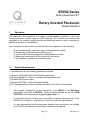
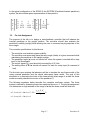
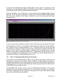
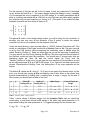
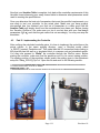
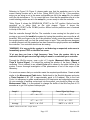
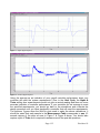
SRV02-Series
Rotary Experiment # 7
Rotary Inverted
Pendulum
Student Handout
SRV02-Series
Rotary Experiment # 7
Rotary Inverted Pendulum
Student Handout
1.
Objectives
The objective in this experiment is to design a state-feedback controller for the rotary
inverted pendulum module using the LQR technique. The controller will maintain the
pendulum in the inverted (upright) position and should be robust in order to maintain its
stability in the case of a disturbance.
Upon completion of the exercise, you should have have experience in the following:
•
•
•
•
•
2.
How to mathematically model the rotary inverted pendulum system.
To linearize the model about an equilibrium point.
To use the LQR method in designing a state-feedback controller.
To design and simulate a WinCon controller for the system.
To use feedback to stabilize an unstable system.
System Requirements
To complete this Lab, the following hardware is required:
[1] Quanser UPM 2405/1503 Power Module or equivalent.
[1] Quanser MultiQ PCI / MQ3 or equivalent data acquisition card.
[1] Quanser SRV02 servo plant.
[1] Quanser ROTPEN – Rotary Pendulum Module.
[1] PC equipped with the required software as stated in the WinCon user manual.
•
The required configuration of this experiment is the SRV02 in the High-Gear
configuration along with a ROTPEN – Rotary Pendulum Module as well as a UPM
2405/1503 power module and a suggested gain cable of 1.
•
It is assumed that the student has successfully completed Experiment #0 of the
SRV02 and is familiar in using WinCon to control the plant through Simulink.
•
It is also assumed that all the sensors and actuators are connected as per dictated
in the SRV02 User Manual and the Rotary Pendulum User Manual.
Page # 2
Revision: 01
3.
Mathematical Model
Figure 1 below depicts the Rotary inverted pendulum module coupled to the SRV02 plant
in the correct configuration. The Module is attached to the SRV02 load gear by two
thumbscrews. The Pendulum Arm is attached to the module body by a set screw. The
Inverted Pendulum experiment is a classical example of how the use of control may be
employed to stabilize an inherently unstable system. The Inverted pendulum is also an
accurate model in the pitch and yaw of a rocket in flight and can be used as a benchmark
for many control methodologies.
Figure 1 - SRV02 w/ ROTPEN Module
The following table is a list of the nomenclature used is the following illustrations and
derivations.
Symbol Description
Symbol Description
L
Length to Pendulum's Center of h
mass
Distance of Pendulum Center
of mass from ground
m
Mass of Pendulum Arm
Jcm
Pendulum Inertia about its
center of mass
r
Rotating Arm Length
Vx
Velocity of Pendulum Center
of mass in the x-direction
θ
Servo load gear angle (radians)
Vy
α
Pendulum Arm Deflection (radians)
Velocity of Pendulum Center
of mass in the y-direction
Page # 3
Revision: 01
Figure 2 - Top View of Rotary inverted pendulum
Figure 3 - Side View with Pendulum in Motion
Figure 2 above depicts the rotary inverted pendulum in motion. Take note of the direction
the arm is moving. Figure 3 depicts the pendulum as a lump mass at half the length of the
pendulum. The arm is displaced with a given α. Notice that the direction of θ is now in the
x-direction of this illustration. We shall begin the derivation by examining the velocity of
the pendulum center of mass.
Referring back to Figure 3, we notice that there are 2 components for the velocity of the
Pendulum lumped mass:
V Pendulum center of mass=−L cos  ̇ x −L sin   ̇ y
[3.1]
We also know that the pendulum arm is also moving with the rotating arm at a rate of:
V arm=r ̇
[3.2]
Using equations [3.1] & [3.2] and solving for the x & y velocity components:
V x=r −L cos  ̇
[3.3]
V y=−L sin   ̇
Equation [3.3] leaves us with the complete velocity of the pendulum. We can now proceed
to derive the system dynamic equations.
Page # 4
Revision: 01
3.1
Deriving The System Dynamic Equations
Now that we have obtained the velocities of the pendulum, the system dynamic equations
can be obtained using the Euler-Lagrange formulation. We obtain the Potential and
Kinetic energies in our system as:
Potential Energy - The only potential energy in the system is gravity:
V =P.E. Pendulum= m g h = m g L cos
[3.4]
Kinetic Energy - The Kinetic Energies in the system arise from the moving hub, the
velocity of the point mass in the x-direction, the velocity of the point mass in the ydirection and the rotating pendulum about its center of mass:
T =K.E. HubK.E. Vx K.E. Vy K.E. Pendulum
[3.5]
*Note: Since we have modeled the pendulum as a point mass at its center of mass, the
total kinetic energy of the pendulum is the kinetic energy of the point mass plus the
kinetic energy of the pendulum rotating about its center of mass.
The moment of inertia of a rod about its center of mass is:
J cm=
1
M R2
12
since we've defined L to be half the pendulum length, then R in this case would be equal
to 2L. Therefore the moment of inertia of the pendulum about its center of mass is:
J cm=
1
1
1
2
2
2
M R = M 2L = M L
12
12
3
[3.6]
Finally, our complete kinetic energy T can be written as:
1
1
1
1
2
2
2
2
T = J eq ˙  m r ̇−L cos  ̇  m −L sin   ̇  J cm ˙
2
2
2
2
[3.7]
After expanding equation [3.7] and collecting terms, we can formulate the Lagrangian:
1
2
1
L=T −V = J eq ˙2 m L 2 ˙ 2−mLr cos  ̇ ̇ m r 2 ˙2−mgLcos
2
3
2
Page # 5
[3.8]
Revision: 01
Our 2 generalized co-ordinates are θ and α. We therefore have 2 equations:

t

t
 
 
L
L
−
=T output−B eq ̇
 ̇

[3.9]
L
L
=0
−
 ̇

[3.10]
Solving Equations [3.9] & [3.10] and linearizing about α = 0, we are left with :
J eq mr 2  ̈−mLr ̈=T output−B eq ̇
[3.11]
4
mL 2 ̈−mLr ̈−mgL =0
3
[3.12]
Referring back to Experiment # 1 – Position Control, we know that the output Torque on
the load from the motor is:
T output =
m  g K t K g V m−K g K m 
[3.13]
Rm
Finally, by combining equations [3.11], [3.12] & [3.13], we are left with the following statespace representation of the complete system:
[ ][
0
0
0
0
bd
E
ad
E
̇
̇
= 0
̈
̈
0
1
0
−cG
E
−bG
E
][ ]
0
1
0
0
0
0
m  g K t K g


 c
Rm E
̇
  K K
̇
b m g t g
Rm E
Vm
Where:
a=J eq mr
b=mLr
4
2
c= m L
3
d=mgL
2
2
E =ac−b
2
 m  g K t K m K g B eq R m
G=
Rm
Page # 6
Revision: 01
In the typical configuration of the SRV02 & the ROTPEN (Pendulum/inverted pendulum)
system, the above state space representation of the system is:
[ ][
][ ] [ ]
̇
0
0
1
0
̇
0
0
0
1
=
0
39.32
−14.52
0
̈
0 81.78 −13.98 0
̈
3.2

0

0

Vm
25.54
̇
24.59
̇
Pre Lab Assignment
The purpose of the lab is to design a state-feedback controller that will balance the
inverted pendulum in the upright position. The controller should also maintain the
pendulum's stability (upright) while allowing the user to command varying setpoints of the
servo angle.
The controller specifications for this lab are:
•
•
•
•
•
The controller must maintain system stability.
The controller must accurately place the servo angle (theta) at a given command while
maintaining the pendulum in the upright position.
The pendulum angle (α) must not exceed ±6° when the system is excited with a step
input to the θ command.
The control signal (Vm) must be strictly bounded by ±2.5 Volts.
The settling times of θ & α should not exceed 2 s each for a step input (θ command of
1 rad).
The first task upon entering the laboratory will be to simulate the non-linear model of the
rotary inverted pendulum and the above state-space linear model. The goal of this
simulation is to determine the limits of the linear model (what range of α does the linear
model accurately describe the motion of the pendulum?).
The following equations below describe the complete non-linear system. The linear
system is derived by linearizing these two equations about α = 0. The pre-lab assignment
is to determine a rough estimate of the range of α that the linear model will hold true.
  K K
2
a ̈−b cos ̈b sin  ˙ G ̇= m g t g V m
Rm
c ̈−b cos ̈−d sin =0
Page # 7
Revision: 01
4.
In Lab Procedure
The Rotary inverted pendulum is an ideal experiment when introducing important controls
concepts such as disturbance rejection and non-linear systems. The intent of this
laboratory is to first validate the use of the linear model (through simulation) and then
proceed to design a closed-loop full state feedback controller that will maintain the
pendulum in its upright position. The inverted pendulum has many practical applications
in that it can be used to model many non-linear systems.
The purpose of the lab is to design a state-feedback controller that will balance the
inverted pendulum in the upright position. The controller should also maintain the
pendulum's stability (upright) while allowing the user to command varying setpoints of the
servo angle.
The controller specifications for this lab are:
•
•
•
•
•
The controller must maintain system stability.
The controller must accurately place the servo angle (theta) at a given command while
maintaining the pendulum in the upright position.
The pendulum angle (α) must not exceed ±6° when the system is excited with a step
input to the θ command.
The control signal (Vm) must be strictly bounded by ±2.5 Volts.
The settling times of θ & α should not exceed 2 sec each for a step input (θ command
of 1 rad).
4.1
Part I - Verification of the Linear Model
The first part of this lab will be verifying our linear model by simulating the linear and nonlinear systems together and looking for the point of divergence. This exercise will not only
verify our linear model, but will also establish a threshold to turn the controller off when α
exceeds the threshold.
The first task upon entering the laboratory is to familiarize yourself with the system. The
pendulum deflection signal (α) should be connected to encoder channel #1 and the
servomotor's position signal (θ) should be connected to encoder channel #0. Analog
Output channel #0 should be connected to the UPM (Amplifier) and from the amplifier to
the input of the servomotor. This system has one input (Vm) and two outputs (θ & α).
You are now ready to begin the lab. Launch MATLAB from the computer connected to
the system. Under the “SRV02_Exp7_Inverted Pendulum” directory, begin by running the
file by the name “Setup_SRV02_Exp7.m”. This MATLAB script file will setup all the
specific system parameters and will set the system state-space matrices A,B,C & D. You
are now ready verify the linear model.
Under the same directory, open a Simulink model called “s_SRV02_Non_Linear_
Pendulum.mdl”. This model is a simulation of the complete non-linear pendulum system
Page # 8
Revision: 01
as well as the linearized state-space representation of the system. The purpose of this
simulation is to investigate the validity of the linear model and also to determine the range
of α where the linear model correctly describe the system.
Start the simulation. You should have 2 scopes open that are displaying alpha (α) and
theta (θ). To put the plots in perspective, α was given an initial condition slightly greater
than 0 and thus allowed to fall. Figure 4 Below is a plot of the linear and non_linear
simulations of α.
Figure 4 - Simulation of Non-Linear & Linear Models
As you can seen from the above simulation, the linear model correctly depicts the motion
of the pendulum for the first 1.5 seconds and then begins to break down. In the simulation
plot of alpha, zoom into graph between 1.4 & 1.6 seconds. Here you will see the two
curves begin to diverge. It seems that the linear model quite accurately describes the
system for the first 25º and then begins to diverge from the actual motion. We will
therefore set the Alpha_Threshold variable to 25º. It should be noted that a range of ±25º
is quite acceptable for this application as the controller you will be designing will try to
maintain the pendulum in the upright position ( α = 0).
4.2
Part II – Designing & Simulating the Controller
Now that we have verified the linear model to be accurate in the range of motion we are
expecting, you will now use this linear model to design a full-state feedback controller to
maintain the pendulum in the upright position and to meet the controller specifications
mentioned above. The method of calculating the feedback gains will be the LQR function
in MATLAB's control systems toolbox.
The MATLAB LQR function returns a set of calculated gains based on the system
matrices A & B and the design matrices Q & R. In this section of the Lab, you will begin
the iterative design process by varying Q and taking notice on the effect those changes
have on the simulated system response.
Page # 9
Revision: 01
For the purpose of this lab, we will fix the Q matrix to only be comprised of 2 elements
(q1,q2) and we will hold R at 1. The reason behind limiting the design to only 2 variables
is to investigate the role of emphasis in an LQR design. q1 is mainly associated with θ
while q2 is mainly associated with α. With this in mind, the user can select which variable
the controller will put more emphasis on forcing to 0. (The result of any stable full-state
feedback controller will be to drive all states to 0).
[ ]
q1 0
0 q2
Q=
0 0
0 0
0
0
0
0
0
0
0
0
The above Q matrix is the simple design matrix you will be using for this controller. In
actuality, the user may vary all the elements of the Q matrix to obtain the optimal
controller, but this is not necessary for the purpose of this lab.
Under the same directory, open a model called “s_SRV02_Inverted_Pendulum.mdl”. This
model is a simulation of the Linear model with a feedback law u = -kx. The gain vector k
is set by the LQR function. Before beginning the simulation, open a Matlab script file
called “Iteration_RotPen.m”. Keep this script open as you will be executing it repetitively.
You may save & run this file by pressing the F5 key. Run this script and then proceed to
the Simulink model and start the simulation. You should have 3 scopes open that are
displaying alpha (α), theta (θ) and the control signal (u). Every time the
“Iteration_RotPen.m” script runs, you will see the new response in the simulation as well
as two step-responses (θ & α) in MATLAB figures. If you right-click on these figures and
choose Characteristics->Settling Time, the settling-time of the step response will be
shown.
The default Q values are Q = diag ([1 1 0 0]) as you can see in the Iteration script. At this
point, you should start varying q1 & q2 and making note of their effect on the closed loop
system characteristics (θ settling time, α settling time, α range, u range). By the end of
this exercise you should have a table of the form:
q1
q2
Theta (θ)
Settling time (s)
Alpha (α)
Settling time (s)
Alpha Range
Control Signal (u)
Range
1
1
2.55
2.65
- 3.2º < α < 3.2º
-1V< u <1V
10
1
1.1
1.51
- 7.2º < α < 7.2º
- 3.2 V < u < 3.2 V
1
10
2.55
2.67
- 2.9º < α < 2.9º
-1V< u <1V
Table 1 - Iteration Table : Sample Entries
Table 1 above shows 3 different entries into the Iteration Table that you should be
constructing. In total there should be 20 entries in the table (vary each parameter in 10
steps while holding the other parameter at 1). Suggested ranges for this exercise are:
0 < q1 < 20 ; 0 < q2 < 50
Page # 10
Revision: 01
Now that your Iteration Table is complete, look back at the controller requirements of this
lab while cross-referencing your newly formed table to determine what parameters would
result in meeting the specifications.
Once you determine the best set of parameters that meet the specified requirements, you
are ready to test your controller on the actual plant. Make sure you have properly
documented how you obtained your final set of parameters in a table much like the
Iteration Table and clearly show how the requirements have been met. Before closing
the “Iteration_RotPen.m” file, make sure you run it one last time with your final design
parameters (q1 & q2) such that the gain vector k is set accordingly. You may now stop the
simulation.
4.3
Part III - Implementing the Controller
After verifying the calculated controller gains, it is time to implement the controllers on the
actual system. In the same working directory, open a Simulink model called
“q_SRV02_Inverted_Pendulum.mdl”. This model has the I/O connection blocks linking to
the physical plant as well as a simulated block to compare real and simulated results.
You may now proceed to “Build” the controller through the WinCon menu. Before
starting the controller, make sure that the pendulum rod is in its correct staring position.
The starting position of the pendulum should match the setting given in the experiment
setup file “Setup_SRV02_Exp7.m”. Open this file and scroll to the following section:
% ############### USER-DEFINED PENDULUM CONFIGURATION ##################################
% Pendulum Start Position: set to 'UP' or 'DOWN'
PENDULUM_START = 'UP';
% ############### END OF USER-DEFINED PENDULUM CONFIGURATION ##########################
Figure 6 - PENDULUM_START = 'UP'
Figure 5 - PENDULUM_START = 'DOWN'
Page # 11
Revision: 01
Referring to Figure 5 & Figure 6, please make sure that the pendulum arm is in the
correct starting location as is set in the “Setup_SRV02_Exp7.m” file. If the pendulum
setup you are using is not in the same configuration as set in the setup file, you should
notify the lab technician or T.A. to correct the error. Now that the pendulum arm is in the
correct starting position as set in the setup file, you are ready to start the controller.
*Note: Figure 6 shows the PENDULUM_START in the 'UP' position. Notice how the
pendulum ar is sitting flush on the right stopper. Figure 5 shows the
PENDULUM_START in the 'DOWN' position. Notice how the pendulum arm is fastened
to the tip of the shaft.
Start the controller through WinCon. The controller is now running but the plant is not
moving as you must first enable the system by having the pendulum arm cross the α = 0
threshold. With one finger on the tip of the pendulum, slowly move the pendulum toward
the upright position until you feel the system begin to work. This controller was designed
to remain dormant until the pendulum arm has crossed the upright position and enabled
the controller. Your controller should now be running.
*WARNING: If at any point the system is not behaving as expected, make sure to
immediately press STOP on the WinCon server.
*If at any time you hear a high frequency 'hum' from the system, this is an
indication that the gains are too high and you need to re-calculate your controller.
Through the WinCon server, open a plot of 3 signals (Measured Alpha, Measured
Theta & Control Signal). You should be noticing the postion of the servo (Theta) is
oscillating. This is referred to as a Limit Cycle and is cause by the static friction in the
system. A more thorough investigation of this phenomenon is out of the scope of this
laboratory.
You must now ensure that you controller meets the required specifications. Create a table
similar to the Measurement Table below. Switch back to the Simulink diagram and enter
a Theta Setpoint of 28° (28° is approximately equal to 0.5 radians). Due to the Limit
Cycle, it is necessary to gather measurements of 5 step inputs and compute the average.
As your controller is sending a step-input into the system, you should be filling out your
Measurement Table. It is recommend to change the buffer of the WinCon plots to 10
seconds as to get 2 full cycles of data per plot.
Sample #
Alpha Range
Control Signal (u) Range
1
-4.5 º < α < 5.5º
-2V< u <2V
..
..
..
5
-4.7 º < α < 5.3º
- 2.2 V < u < 2.2 V
Average
-4.63 º < α < 5.4º
- 2.05 V < u < 2.1 V
Table 2 - Measurement Table - Sample Entries
Page # 12
Revision: 01
Figure 7 - Alpha Signal Capture
Figure 8 - Control Signal Capture
Using the average as an indication of your overall controller performance, does your
controller still meet the system requirements? (Due to the Limit Cycle, the Alpha &
Theta settling time measurements would not give an actual reading and thus not be an
accurate indication of controller performance. If your controller did not manage to meet
the specified requirements, you should go back to the simulations and re-iterate the
design procedure until you have developed a controller that will meet the requirements.
The previous figures show the WinCon plots used to make the above calculations. It
should be noted that each sample in the Measurement Table corresponds to one 10second capture of the plots as seen in Figure 7 & Figure 8 above. You should also
capture a plot of Theta as it is required to answer some of the post-lab questions.
Page # 13
Revision: 01
5.
Post Lab Question and Report
Upon completion of the lab, you should begin by documenting your work into a lab report.
Included in this report should be the following:
i.
In the pre-lab, you were asked to theorize as to the range of alpha that you would
expect the linear model to be valid. Include all calculations and the final estimate.
ii.
In Part II of the lab, you were asked to vary 2 parameters (10 steps for each) for a
total of 20 entries. Make sure to include your Iteration Table in this report.
iii.
With the controller requirements in mind, you were asked to determine the optimal
parameters to achieve those specifications. Include your design steps and all
iterations used in determining the final controller.
iv.
After implementing your designed controller on the real plant in Part III of the lab,
you were asked to compile a Measurement Table. Make sure this is included in
your final report.
v.
In Part III, you implemented your controller on the physical plant. Comment on the
performance of your controller on the actual system as opposed to the simulated
model.
vi.
Make sure to include your final controller gains and any re-iterative calculations
made if any.
5.1
Post Lab Questions
1) Having performed this lab by using the LQR technique, what other control approaches
would you consider for this system?
2) The inverted pendulum is a classical example of a non-minimum phase system. In
what way is this true. Prove your argument with plots from the actual plant.
3) By how much did your measurements of the actual controller deviate from those of the
simulated model? Give some quantitative measurements and comment on what you
perceive as being the source of these discrepancies.
4) Once you implemented your controller on the actual system, you should have noticed
the Limit Cycle phenomenon. What ways would there be of incorporating this into your
model so that it would show up in the simulations.
Page # 14
Revision: 01