1
SRV02-Series Rotary Experiment # 4 Flexible Joint Student Handout SRV02-Series Rotary Experiment # 4 Flexible Joint Student Handout 1. Objectives The objective in this experiment is to design a state-feedback controller for the rotary flexible joint module which allows you to command a desired tip angle position. The controller should eliminate the arm's vibrations while maintaining a fast response. Upon completion of the exercise, you should have experience in the following: • • • • • 2. How to mathematically model the flexible joint system. To linearize the model about an operating point. To dampen the arm vibrations with full-state feedback. To design and simulate a WinCon controller for the system. How to design an optimal LQR controller. System Requirements To complete this Lab, the following hardware is required: [1] Quanser UPM 2405/1503 Power Module or equivalent. [1] Quanser MultiQ PCI / MQ3 or equivalent. [1] Quanser SRV02 Servo plant. [1] Quanser ROTFLEX – Rotary Flexible Joint Module. [1] PC equipped with the required software as stated in the WinCon user manual. • The required configuration of this experiment is the SRV02 in the High-Gear configuration along with a ROTFLEX – Rotary Flexible Joint module as well as a UPM 2405/1503 power module and a suggested gain cable of 1. • It is assumed that the student has successfully completed Experiment #0 of the SRV02 and is familiar in using WinCon to control the plant through Simulink. • It is also assumed that all the sensors and actuators are connected as per dictated in the SRV02 User Manual and the Rotary Flexible Joint User Manual. Page # 2 Revision: 01 3. Mathematical Model Figure 1 below depicts the Flexible Joint module coupled to the SRV02 plant in the correct configuration. The Module is attached to the SRV02 load gear by two thumbscrews. The Main Arm is attached to the module body by two identical springs thus resulting in the flexible joint. Figure 2 shows the different anchor points on the body and the arm resulting in many configurations of the module. Figure 1 - Flexible Joint Module Figure 2 - Flexible Joint Illustration The following table is a list of the nomenclature used is the following illustrations and derivations. Symbol Description Symbol Description R Distance from joint to arm anchor L1, L2 Lengths of Spring #1 & #2 d Distance from joint to body anchor F1, F2 Forces on Spring #1 & #2 r Fixed distance (r = 3.18 cm) k Spring Stiffness θ Servo load gear angle (radians) L Unstretched Spring Length α Arm Deflection (radians) M Restoring Moment Page # 3 Revision: 01 Figure 3 - Flexible Joint - Stationary Figure 4 - Flexible Joint - Moving Figure 3 above depicts the joint at rest while Figure 4 depicts the joint at a given α. Notice that spring #1 has been compressed and spring #2 has been stretched (with respect to the joint's stationary state). We shall begin by deriving the lengths of each spring in Figure 4. L 1x =r−Rsin L 1y =Rcos −d L 2x =rRsin L 2y =L 1y =Rcos −d L 1= L 21x L 21y 2 [3.1] 2 L 2= L 2x L 2y Next we will derive the force acting on each spring: F 1=K L 1−LF r F 2=K L 2−L F r L L F 1x =F 1 1x , F 1y =F 1 1y L1 L1 L L F 2x =F 2 2x , F 2y =F 2 2y L2 L2 [3.2] * Fr is the restoring force on each spring. The springs supplied come pre-loaded meaning they will not stretch before the force Fr is applied. Page # 4 Revision: 01 Referring back to Figure 4, we can see that F1 & F2 are both acting on the Arm anchor point (The point where both springs are attached to the arm). By simple inspection, we can see that the x components are opposing each other while the y components are in the same direction leaving us with: F x=F 2x −F 1x F y=F 2y F 1y [3.3] We now have 2 forces acting on the anchor point that will bring the arm back to its original position. These 2 forces will cause a torque about the joint. We know that the torque (restoring Moment) is equal to the cross product of the radius R and each force resulting in the following: M x=R x F x=R F x sin /2−=R F x cos M y=R x F y=R F y sin 2 −=−R F y sin [3.4] M =M xM y=R cos F 2x −F 1x −R sin F 2y F 1y We now have our restoring moment M. We will be modeling the flexible joint as a simplified spring with the following dynamic equation. M =K Stiff Figure 5 below shows the simplified model that will be used for the flexible joint. Since M is non-linear, we can get a linear 1st order linear estimate of the joint stiffness Kstiff : K Stiff = M , evaluated at=0 *For a complete and detailed derivation of the linear joint stiffness, please refer to the Maple file “K_Stiff_Linear.mws”. The final derivation as obtained from maple is: K Stiff =[ 2R D 3/ 2 ][Dd−Rr 2 F r D3 / 2 d−DLdRr 2 L K ] [3.5] Figure 5 - Simplified Model for System Dynamics Page # 5 Revision: 01 3.1 Deriving The System Dynamic Equations Now that we have developed a linear model for the joint, the system dynamic equations can be obtained using the Euler-Lagrange formulation. We obtain the Potential and Kinetic energies in our system as: Potential Energy - The only potential energy in the system is in the spring: 1 V =P.E. Spring = K Stiff 2 2 [3.6] Kinetic Energy - The Kinetic Energies in the system arise from the moving hub and flexible arm: 1 1 2 2 T =K.E. HubK.E. Arm= J eq ˙ J Arm ̇̇ 2 2 [3.7] Forming the Lagrangian: 1 1 1 L=T −V = J eq ˙2 J Arm ̇̇2− K Stiff 2 2 2 2 [3.8] Our 2 generalized co-ordinates are θ and α. We therefore have 2 equations: t t L L =T output −Beq ̇ − ̇ [3.9] L L − =0 ̇ [3.10] Solving Equations [3.9] & [3.10], we are left with : J eq ̈J Arm ̈̈=T output −B eq ̇ [3.11] J Arm ̈̈K Stiff =0 [3.12] Referring back to Experiment # 1 – Position Control, we know that the output Torque on the load from the motor is: T output = m g K t K g V m−K g K m ̇ [3.13] Rm Page # 6 Revision: 01 Finally, by combining equations [3.11], [3.12] & [3.13], we are left with the following statespace representation of the complete system: [] 0 0 0 0 ̇ K Stiff ̇ = 0 J eq ̈ ̈ −K Stiff J eq J Arm 0 J eq J Arm 3.2 1 0 0 1 2 − m g K t K m K g B eq Rm J eq R m 0 2 m g K t K m K g B eq Rm J eq R m 0 [] 0 0 m g K t K g J eq R m ̇ − m g K t K g ̇ Vm J eq R m Pre Lab Notes The purpose of the lab is to design a state-feedback controller that will place the tip of the arm (θ + α) at a given command. The controller must also meet the following criteria: • • • The controller's response to a step-input should have a maximum rise-time of 250 ms. There should be a maximum of 5% overshoot. The Arm deflection should never exceed 10˚. (-10˚ < α < 10˚). The following lab will be divided into two parts. There will first be a design and simulation section that will entail a number of iterations and simulations of the controller. In this section, the student will be required to design a full state feedback controller using the LQR method to calculate the gains. The student should come into the lab with a theoretical understanding of LQR as well as a functional understanding of MATLAB. Part II of the laboratory will consist of implementing the final controller on the physical plant (SRV02-Flexible Joint), as well as comparing the performance of the full-state feedback controller as opposed to a controller with feedback only from the servo-motor. This section will also entail some frequency analysis on both closed-loop models so an understanding of natural frequencies and resonance will also be required. Page # 7 Revision: 01 4. In Lab Procedure The rotary flexible joint is an ideal experiment intended to model a flexible joint on a robot or spacecraft. This experiment is also useful in the study of vibration analysis and resonance. The purpose of the lab is to design a state-feedback controller that will place the tip of the arm (θ + α) at a given command. The controller must also meet the following criteria: • • • The controller's response to a step-input should have a maximum rise-time of 250 ms. There should be a maximum of 5% overshoot. The Arm deflection should not exceed 10˚. (-10˚ < α < 10˚). 4.1 Part I - Design & Simulation The first part of this lab will be to design a state-feedback controller that will meet the required specifications. The method of calculating the feedback gains will be the LQR function in MATLAB's control systems toolbox. The first task upon entering the laboratory is to familiarize yourself with the system. The arm deflection signal (α) should be connected to encoder channel #1 and the servomotor's position signal (θ) should be connected to encoder channel #0. Analog Output channel #0 should be connected to the UPM (Amplifier) and from the amplifier to the input of the servomotor. This system has one input (Vm) and two outputs (θ & α). You are now ready to begin the lab. Launch MATLAB from the computer connected to the system. Under the “SRV02_Exp4_Flexible Joint” directory, begin by running the file by the name “Setup_SRV02_Exp4.m”. This MATLAB script file will setup all the specific system parameters and will set the system state-space matrices A,B,C & D. You are now ready to begin the design process. The MATLAB LQR function returns a set of calculated gains based on the system matrices A & B and the design matrices Q & R. In this section of the Lab, you will begin the iterative design process by varying Q & R and taking notice on the effect those changes have on the simulated system response and the closed-loop poles (eigen values). For the purpose of this lab, we will fix the Q matrix to be only diagonal. This will allow you to vary 4 parameters for Q (q1,q2,q3,q4) and one parameter for R (r1) (R in this case is scalar as there is only 1 input and therefore 1 control signal). [ ] q1 0 0 0 0 q2 0 0 Q= , 0 0 q3 0 0 0 0 q4 R=r 1 Page # 8 Revision: 01 Under the same directory, open a Simulink model called “s_SRV02_Flexible_Joint.mdl”. This model is a simulation of the Flexible Joint system with a feedback law u = -kx. The gain vector k is set by the LQR function. Before beginning the simulation, open a Matlab script file called “Iteration_RotFlex.m”. Keep this script open as you will be executing it repetitively. You may save & run this file by pressing the F5 key. Run this script and then proceed to the Simulink model and start the simulation. You should have 3 scopes open that are displaying alpha (α), theta (θ) and gamma (θ + α). Every time the “Iteration_RotFlex.m” script runs, you will see the new response in the simulation as well as a step-response of the arm-tip position (θ + α) in a MATLAB figure. If you right-click on this figure and choose Characteristics->Rise Time, the rise-time of the step response will be shown. Switching back to your MATLAB command window, you should see the calculated gain vector k, as well as the corresponding closed-loop eigenvalues (poles) E. The default Q & R values are Q = diag ([10 100 1 1]) & R = 1 as you can see in the Iteration script. You should notice that the largest value in Q is q2. This should be of no surprise as the emphasis of the controller should be primarily on keeping α as close to 0 as possible. Therefore, the largest element of Q should be the one that is associated with α. At this point, you should be varying the components of Q & R and making note of their effect on the closed loop system characteristics (rise time, overshoot, α range). By the end of this exercise you should have a table of the form: q1 q2 q3 q4 r Rise time (ms) % Overshoot Alpha Range 10 100 1 1 1 771 0 - 4º < α < 4º 100 100 1 1 1 137 9.32 % - 13º < α < 13º 10 1 0 0 0.1 104 15.2 % - 20º < α < 20º Table 1 - Iteration Table : Sample Entries Table 1 above shows 3 different entries into the Iteration Table that you should be constructing. In total there should be 25 entries in the table (vary each parameter in 5 steps while holding the other parameters constant). For an idea of what values to simulate, refer to the following table for suggested ranges: Parameter q1 q2 q3 q4 r Range 0 < q1 < 500 0 < q2 < 2000 0 < q3 < 10 0 < q4 < 20 0.1 < r < 10 Table 2 - Suggested Parameter Ranges As you proceed with your iterations, take note of the closed-loop eigenvalues (poles) as you vary each parameter. By the end of your 25 iterations, you should have a qualitative understanding of how each parameter affects the closed loop poles. Now that your Iteration Table is complete, look back at the controller requirements of this lab while cross-referencing your newly formed table to determine what parameters would result in meeting the specifications. Page # 9 Revision: 01 Once you determine the best set of parameters that meet the specified requirements, you are ready to test your controller on the actual plant. Make sure you have properly documented how you obtained your final set of parameters in a table much like the Iteration Table and clearly show how the requirements have been met. You may now stop the simulation. 4.2 Part II - Implementing the Controller After verifying the calculated controller gains, it is time to implement the controllers on the actual system. In the same working directory, open a Simulink model called “q_SRV02_Flexible_Joint.m”. This model has the I/O connection blocks linking to the physical plant as well as a simulated block to compare real and simulated results. Figure 6 - Flexible Joint Controller Figure 6 above depicts the Rotary Flexible Joint controller we have developed for this experiment. Notice that both the actual system and an exact simulation are running in parallel thus allowing us to compare the actual and simulated results. Before “Building” this controller, make sure that the state-feedback gain k is set according to your final design parameters. You may now proceed to “Build” the controller through the WinCon menu. After the code has compiled, start the controller through WinCon and open up two scopes; one for alpha (measured and simulated together) and another for gamma (measure and simulated together). Page # 10 Revision: 01 *WARNING: If at any point the system is not behaving as expected, make sure to immediately press STOP on the WinCon server. *If at any time you hear a high frequency 'hum' from the system, this is an indication that the gains are too high and you need to re-calculate your controller with a larger R. • • How close do the simulated and measured responses match? By first inspection, would you say that the controller you designed has met the requirements? The following two figures show the measured and simulated response of gamma (Figure 7) and alpha (Figure 8). As you can clearly see, all the design objectives have been met. Figure 7 - Measured & Simulated Gamma Plot Figure 8 - Measured & Simulated Alpha Plot Page # 11 Revision: 01 If your measured values do not meet the requirements (for instance if the measured alpha exceeds 10°), you will have to re-iterate your controller and try again. Remember to first simulate before implementing the new controller on the actual plant. When your controller meets the required specifications, make sure to print your plots. They should look similar to Figures 7 & 8. You have now successfully designed a full-state feedback controller using LQR. The following exercises are meant to illustrate how useful this technique is in suppressing the arm vibrations. In the same working directory, open the “q_SRV02_ROTFLEX_Vibration.mdl” model. Build, and run this model. This model alternates between the full-state feedback controller you just designed and a PD controller with no deflection feedback ( k(2) & k(4) are set to 0 every other period). By observing the plant, you should notice how well the full-state feedback controller effectively eliminates all arm vibrations. To further demonstrate the effects of full-state feedback on the arm deflection, we will send a chirp signal input (a sinusoid with increasing frequency) to both controllers. Figure 9 shows the arm position (α) when there is no deflection (notice the resonant frequency). Figure 10 shows the arm position when there is full-state feedback. Notice how the resonant peak is completely removed and the vibrations are minimal using the full-state feedback. Both plots were obtained by a variable frequency sine wave with amplitude of 10°. Figure 9 - Sine Sweep Response without deflection feedback Figure 10 - Sine Sweep Response with Full-State Feedback Page # 12 Revision: 01 5. Post Lab Question and Report Upon completion of the lab, you should begin by documenting your work into a lab report. Included in this report should be the following: i. In Part I of the lab, you were asked to vary 5 parameters (5 steps for each) for a total of 25 entries. Make sure to include your Iteration Table in this report. ii. As you filled out the Iteration Table, you were asked to qualitatively take note on the location of the closed-loop poles (E) as you varied each parameter. You should include in this report a brief description on what effects the variation of each parameter had on the poles. (ex: poles went further to the left, imaginary components became larger, etc.) iii. With the controller requirements in mind, you were asked to determine the optimal parameters to achieve those specifications. Include your design steps and all iterations used in determining the final controller. iv. After implementing your designed controller on the real plant in Part II of the lab, include your plots of gamma and alpha. These plots should be look similar to Figures 7 & 8. If you had to re-iterate your design after implementation, include ALL plots from each iteration. v. In Part II, you implemented your controller on the physical plant. Comment on the performance of your controller on the actual system as opposed to the simulated model. vi. Make sure to include your final controller gains and any re-iterative calculations made if any. 5.1 Post Lab Questions 1) After completing your Iteration Table, you should now be fairly familiar with how to setup the Q & R matrices to achieve the optimal controller. What intuitive reasoning on choosing the Q & R matrices have you learnt from the completion of this lab. What are the important considerations when using the LQR technique in calculating the full-state feedback gains. 2) Having an insight into the location of the closed loop poles as you varied your parameters, would you have chosen a pole-placement technique to control this plant and meet the required specifications? Are there any other control strategies that you believe could be used to in this lab? 3) In the final section of lab, you were shown how the full-state feedback control could effectively eliminate arm vibrations. When the deflection feedback was turned off ( k(2) & k(4) set to 0 ), there was a resonant frequency at which the arm oscillations were at a maximum (refer to Figure 9). Given only the model of the plant, at what frequency did this resonant peak occur. Remember, you may only use the system state-space Page # 13 Revision: 01 matrices A,B,C & D to determine the resonant frequency. *Hint: Use the Matlab functions SS & Bode to calculate this frequency. Do not forget to set k(2) & k(4) to 0. 4) How closely did your measured and simulated responses match? Did your initial calculated gain k work on the actual plant the first time or did you have to re-iterate your design? Page # 14 Revision: 01