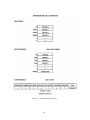
1
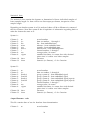
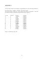
NASA/CR-2002-211440
NASA LaRC FIB Multi-Channel Anemometry
Recording System—User’s Manual
Compiled by:
Sherylene Johnson
NYMA, Inc., Hampton, Virginia
Arild Bertelrud
Analytical Services & Materials, Inc., Hampton, Virginia
February 2002
The NASA STI Program Office . . . in Profile
Since its founding, NASA has been dedicated
to the advancement of aeronautics and space
science. The NASA Scientific and Technical
Information (STI) Program Office plays a key
part in helping NASA maintain this
important role.
The NASA STI Program Office is operated by
Langley Research Center, the lead center for
NASA’s scientific and technical information.
The NASA STI Program Office provides
access to the NASA STI Database, the
largest collection of aeronautical and space
science STI in the world. The Program Office
is also NASA’s institutional mechanism for
disseminating the results of its research and
development activities. These results are
published by NASA in the NASA STI Report
Series, which includes the following report
types:
• TECHNICAL PUBLICATION. Reports of
completed research or a major significant
phase of research that present the results
of NASA programs and include extensive
data or theoretical analysis. Includes
compilations of significant scientific and
technical data and information deemed
to be of continuing reference value. NASA
counterpart of peer-reviewed formal
professional papers, but having less
stringent limitations on manuscript
length and extent of graphic
presentations.
• TECHNICAL MEMORANDUM.
Scientific and technical findings that are
preliminary or of specialized interest,
e.g., quick release reports, working
papers, and bibliographies that contain
minimal annotation. Does not contain
extensive analysis.
• CONTRACTOR REPORT. Scientific and
technical findings by NASA-sponsored
contractors and grantees.
• CONFERENCE PUBLICATION.
Collected papers from scientific and
technical conferences, symposia,
seminars, or other meetings sponsored or
co-sponsored by NASA.
• SPECIAL PUBLICATION. Scientific,
technical, or historical information from
NASA programs, projects, and missions,
often concerned with subjects having
substantial public interest.
• TECHNICAL TRANSLATION. Englishlanguage translations of foreign scientific
and technical material pertinent to
NASA’s mission.
Specialized services that complement the
STI Program Office’s diverse offerings include
creating custom thesauri, building customized
databases, organizing and publishing
research results . . . even providing videos.
For more information about the NASA STI
Program Office, see the following:
• Access the NASA STI Program Home
Page at http://www.sti.nasa.gov
• Email your question via the Internet to
[email protected]
• Fax your question to the NASA STI
Help Desk at (301) 621-0134
• Telephone the NASA STI Help Desk at
(301) 621-0390
• Write to:
NASA STI Help Desk
NASA Center for AeroSpace Information
7121 Standard Drive
Hanover, MD 21076-1320
NASA/CR-2002-211440
NASA LaRC FIB Multi-Channel Anemometry
Recording System—User’s Manual
Compiled by:
Sherylene Johnson
NYMA, Inc., Hampton, Virginia
Arild Bertelrud
Analytical Services & Materials, Inc., Hampton, Virginia
National Aeronautics and
Space Administration
Langley Research Center
Hampton, Virginia 23681-2199
February 2002
Prepared for Langley Research Center
under Contract NAS1-96014
Available from:
NASA Center for AeroSpace Information (CASI)
7121 Standard Drive
Hanover, MD 21076-1320
(301) 621-0390
National Technical Information Service (NTIS)
5285 Port Royal Road
Springfield, VA 22161-2171
(703) 605-6000
Table of Contents
1
General
2
System Instrumentation
5
1.1
1.2
1.3
1.4
1.5
1.6
1.7
1.8
5
5
6
6
6
7
7
7
7
8
9
9
1.9
1.10
2
Exabyte Data
11
2.1
11
11
11
12
12
12
12
12
12
12
13
13
13
15
15
15
15
2.2
3
4
Hot Film Sensors
Anemometer Multiplexers
Anemometers- Dantec/DISA
Filters
DASM Data Acquisition System Management
Port Expander
Time Code Generator-D/A Clock Generator
System Computer
1.8.1 Flight System Start-up Procedures
1.8.2 Flight System Power-down procedures
Analog Back-up System
System Modifications for LTPT
Record Structure
2.1.1 Header
2.1.1.1 DC Offsets
2.1.1.2 Record Counter
2.1.1.3 Channel 8 Identification
2.1.1.4 Gain
2.1.1.5 System A/System B Bank Number
2.1.2 Sampling Groups
Data Retrieval and Conversions
2.2.1 Retrieval Procedures
2.2.1.1 GMT Time Specifications
2.2.1.2 Header Time Adjustment
2.2.2 SUN Computer Data Extraction Procedures
2.2.3 Decoding Embedded Time
2.2.3.1 Seconds from Base Time
2.2.3.2 Bit Orientation
2.2.3.3 Decoding Example
Data Analysis Software Program
17
3.1
17
17
EXABYTEREAD-version 1.0
3.1.1 Running the Code
Data Verification
22
4.1
4.2
4.3
4.4
4.5
22
22
22
23
23
23
DC Offset Conversions
SUN Identifier
Timecode Analysis
Sync Verification of Embedded Timecode
Buffer Time Analysis
4.5.1 Buffer Time Calculations
1
General
The anemometry system was developed to provide high frequency hot film data from a
large number of surface mounted hot film sensors in flight. The system hardware was
built with a pallet going into the LaRC Boeing 737 aircraft cargo bay and a workstation
mounted in the B-737 cabin. The system is flight hardware (built and flight-hardened to
LaRC Flight Specifications per LHB 7910). The hardware is modular and may be used in
ground facilities - it is tracked and used as a complete system.
The purpose of the present description is to provide enough information regarding the
hardware and associated systems used to allow a potential user of the database to assess
the entire system or parts of it as well as to perform data analysis
This documentation is not meant to be an exhaustive description, and the details
regarding hardware and software for engineering analysis have been filed in separate
volumes.
This description is organized in the sequence of the signal flow starting from the sensor
end, going through the signal conditioning, data acquisition, data storage and
subsequent data retrieval.
The system consisted of the following hardware built into two physical entities:
- A pallet with anemometers and analog multiplexing.
- A control rack with signal conditioning, A/D conversion, a SUN
workstation, and two digital Exabyte tape drives for data storage (plus a 14channel analog FM tape recorder).
Anemometers: There were two seven channel Dantec Constant Temperature Anemometers
(without temperature compensation), providing a total of 14 simultaneous channels. The
maximum current per channel is 191 mA, and maximum hot probe resistance (lead plus
sensor) is 30 Ohms. It is necessary to match lead lengths (5 or 20 meters) for inductance
and total resistance due to the analog multiplexing described below.
The anemometry was completely controlled by software on a SUN workstation, and
physically 98 channels (2 systems x 7 channels x 7 groups) are available through analog
multiplexing. If more channels are required, the anemometry may be switched to
‘standby’ and the connectors (4) changed.
Traditionally, transition and turbulence data were obtained through use of high-pass
filtering (AC-coupling) in addition to anti-aliasing filtering (low-pass). In the current
system, both the time-averaged and the time-dependent hot film signals are made
accessible for transition detection, through an analog zero-offset system that removes the
main portion of the time-averaged signal.
This is done through running the anemometry in a zero-offset mode in wind-off
conditions. The system measures the time-averaged voltage, converts it to an 8-bit
integer, which in turn determines a compensation voltage for each channel. The
compensated voltage can then be amplified to the appropriate level (SUN control).
2
This value is part of the information available in the recorded frames of data, and thus
the true voltage at any instance can be recreated (without the low frequency cutoff).
The sampling rate is currently 50 kHz per channel with a 14-bit A/D with sample-andhold, filtering is done with an 8-pole Chebyshev at 20 kHz. If needed, this can be changed
e.g. to Bessel filters (for true signal recording) and the corner frequency may also be
adapted.
The binary data are recorded in parallel on two digital Exabyte recorders, 8 channels per
recorder, on 8 mm tape with a total capacity of 2.5 or 5 gigabytes. Channels 1 through 7
are anemometry, the eighth is time code on system A and group identification on system
B. (Each record on both systems contains a record counter value given by the SUN
computer that ensures synchronization between the two tapes.) The time code is
generated in the SUN computer, and allows time-correlation with tunnel (or flight)
parameters.
Recording is normally done in bursts of 1024 samples over 20 msec, then 20 msec nonrecorded, another 1024 samples, etc. until one buffer consisting of 64 x 8 x 1024 samples has
been filled over 2.62 seconds. When the complete buffer has been transferred to the Exabyte
tape 1.5 seconds later, the buffer begins to fill up again. It is also possible to fill the buffer
through continuous sampling, if a long continuous signal trace is desired. In this case
the buffer is filled in 1.31 seconds. With the 20-msec bursts the minimum frequency (highpass) is 50 Hz, while the continuous has 1.6 Hz.
Switching from sensor group to sensor group switches both bridge feed (i.e. heating the
sensor) and the signal output. It is initiated via the SUN workstation, but the system
will make sure that no switching occurs while filling a buffer. Switching is done by
specifying the groups to be used in system A and B respectively, 1 through 7 each. One
may also have an automatic ‘roll-through’ of all channels over a preset time to simplify
data reduction.
The data reduction is done by specifying the desired start and stop times for data files to
be read, and typically the files are moved over to a Macintosh computer where the
EXABYTEREAD code runs. This code allows ‘stripping out’ selected data segments either
as statistical values only or also as signal samples suitable for frequency analysis. The
data are checked for consistency and synchronization between the two Exabyte tapes, and
the time-code on channel 8 is read to verify when the time data were actually taken (not
when it was recorded).
Output from the EXABYTEREAD code is in the form of ASCII files that use counts or
volts for the dynamic data, and volts for the time-averaged data. The statistical
information is rms (standard deviation), skewness and flatness as well as
autocorrelations and cross correlations between neighboring sensors. The statistics can
be based on anywhere from 16 to 1024 data samples per data set, but there is a
compromise between processing speed and accuracy.
The output files may either be tab-delimited or comma-delimited, depending on the
desired post-processing. In the past customized output file layouts have been provided for
3
quick dissemination of results. A graphics capability exists allowing signal examination,
but the capabilities have been limited to keep the code as general as possible.
A custom-interface exists for wind tunnel work. This consists of a simple graphics
display of output statistics as a function of sensor location, and allows indication of the
transition location through examination of time segments of moderate lengths after each
tunnel run. (The time segment length is determined by the time needed to switch through
the sensors.)
The system covers the entire process hot film anemometry from sensor to statistics
output. Some of the features are readily changed while others are fixed.
The system was developed for use under flight conditions by the NASA LaRC Flight
Instrumentation Branch, with the main contributions made by Carroll Lytle, Carl Mills
and Doug Taylor (NYMA, Inc.) and Sharon Graves (Lockheed-Martin Engineering and
Sciences Corp.), and Keith Harris FIB, (NASA LaRC).
4
1 System Instrumentation
Figure 1 shows the system block diagram. The various parts of the system are described in
the following section.
1.1
Hot Film Sensors
The hot film sensors used in the high-lift experiment were manufactured in the NASA
LaRC Microelectronics and Sensor Development Section. The films were manufactured
from Nickel-coated Upilex film (from UBE, Inc.). To obtain desirable resistance values and
a small sensor size (needed due to the power supply limitations), 0.5 Ohm/square film
was used. The sensors were etched with a 0.003-inch line width and a 0.060-inch length,
giving the films a nominal cold resistance of 10 Ohms. With the substrate heat
conduction applicable to the B-737 High-Lift system, the total area of the sensing
elements should be less than 200 mils due to the power limitations of the anemometry
(based on the desired overheat). A thin layer of Aluminum Oxide was applied to stabilize
the films. Even so, the sensors turned out to be pollution/humidity-sensitive, and in the
flight test series it was necessary to replace entire sheets of the sensors. The sensors
deteriorated over time, with their electrical resistance increasing. In the data reduction,
this has to be taken into account for quantitative analysis. If only dynamic analysis is
performed there is no need for corrections, except to be aware of the general problems
related to the effects of overheat on dynamic response.
There is no problem operating the anemometry system with ordinary hot wires or films
of different resistance, geometric layout, etc. The main problem arises due to the
multiplexing, which sets limitations on the tolerable resistance variation for the sensor
elements.
1.2
Anemometer Multiplexers (See Block Diagram, Figure 1)
A total of 98 sensors can be hooked up to the system at any one time. Since there are only
14 anemometry channels, the prearranged sensors are operated through multiplexers,
where the user can select which of the two groups (of 7 channels each) are being used.
There are two Anemometer Multiplexers, one for the System A hot film sensors and one
for the System B hot film sensors. Forty-nine sensors are input to each multiplexer via
RG-188 coax cables, which are grouped into seven banks of seven sensors. The choice of
group (or bank) is done through use of a six bit character, the three LSB (least significant
bits) of which control the seven banks of System A and the three MSB (most significant
bits) control the seven banks of System B. The character activates one of the systems
when transmitted by the SUN computer and Port Expander. The system selection is
dependent on the Anemometer Multiplexer Control Cards, which are identical in both
systems and differ only in the connection of the jumper hardware.
Since each group/bank has a unique analog voltage which is output through the
Anemometer Switching Control Card to the DASM Channel 8 of System B, which, when
analyzed, provides embedded bank identification in the data.
5
If a large S/N (signal to noise) ratio is desired, bypassing the multiplexer may be a
consideration.
(The DASM is also a multiplexer. See section 1.5 for definition. )
1.3
Anemometers - Dantec/DISA (See Block Diagram, Figure 1)
The Dantec units are responsible for maintaining constant sensor temperature (only
active sensors are heated). This is achieved by an internal bridge and servo amplifier that
monitors the sensor resistance. There are a total of fourteen Dantec/DISA units between
System A and System B each assigned seven channels which controls multiple sensors
switched by one of the two multiplexers. For detailed information on the units see
Instructional Manuals Dantec 56C17-CTA Bridge and 56B10/56B12 Main record.
The bridge has a 1:20 bridge ratio, with a top resistance of 400 Ohms. Maximum
bandwidth is 150 kHz (with 5-meter cable). In the LTPT experiment excessive lead
resistance led to modifications in the bridge circuit (see section 1.10).
The power supply limits the current output from each System (A or B) to 191 mA for
each channel, and it is necessary to ensure that the total heat loss (conduction to the
substrate and convection through air flow) from the sensors used stays below this limit.
(The entire system provides slightly in excess of 1.33 Amps, and if more than 191 mA per
channel is needed, fewer than 7 channels can be used.)
1.4
Filters (See Block Diagram, Figure 1)
For the digital system there is no AC-coupling, i.e. the signal contains the DC voltage (see
1.9 regarding the backup analog system description).
The analog low-pass filters are of type Maxim Max 274, with capability of providing
Chebyshev, Bessel or Butterworth filtering programmed by external resistance.
Pole/Frequency range is 100 Hz to 150 kHz.
The low-pass filters currently being used are of 8th order, continuous-time, analog
Chebyshev filters providing anti-aliasing bandwidth reduction. There are two filter units,
one for System A and one for System B. The system has a sampling rate of 50kHz and the
filters provide a cut-off frequency of 20kHz at the 3dB points. The filter cards also have an
inverting amplifier with a gain of two. Note that the DASM (reference 1.5 & 2.1.2.4) has a
computer-activated gain control in addition to the filter card gain.
1.5
DASM - Data Acquisition System Management (See Block Diagram)
Each SCSI based DASM-AD14 has an eight channel multiplexer followed by a single
input, 14 bit, A/D (analog-to-digital) converter. The DASM provides a 50kHz sampling
per channel (the sampling frequency is flexible - 50kHz was used in both the 737 High-Lift
6
and LTPT projects), the eight analog sample and hold outputs are strobed
simultaneously to the multiplexer. The samples are then sequentially digitized by the
multiplexer at a rate of 2MHz and stored in the DASM until a buffer is completed (the
DASM emulates a read-and-write hard drive). When prompted by the SUN computer the
buffer is read from the DASM over the SCSI bus and written to the Exabyte tape.
1.6
Port Expander (See Block Diagram)
The purpose of the port expander is to take a digital command from the single output port
of the system computer and “expand” it into three outputs, which can address five
devices simultaneously. One output controls both anemometer multiplexers, another
output controls both filters and the remaining output addresses the time code unit.
The port expander is a NASA designed and fabricated subsystem.
1.7
Time Code Generator-D/A Clock Generator (See Block Diagram)
This device generates the data sample clock, which is sent to the DASM and encodes the
parallel time code. The digital parallel time is converted to an analog signal, amplified
and is output to DASM, Unit 1, System A, Channel 8 and is recorded to one of the Exabyte
tapes along with every data sample.
The Time Code Generator-D/A Clock Generator are NASA designed and fabricated
subsystems.
1.8
System Computer (See Block Diagram)
The system computer is a SUN SPARC Station 2 with two Exabyte 8mm tape drives and
two DASM-AD14 SCSI analog-to-digital converters (refer to 1.5 above), one DASM per
Exabyte. The data is retrieved from the DASM and recorded on the Exabyte tape.
The tape transport mechanism is a product of Exabyte, which along with the SCSI
interface is packaged and sold by Contemporary Cybernetics. Any brand of 8mm tape can
be used provided it is data quality and has a storage capacity of 2.5 or 5 gigabytes.
1.8.1 Flight System Start-up Procedures
ANEMOMETER SYSTEM START-UP SHEET
1.) Master Power On
2.)Press in circuit breakers: 2,3,4,6,7,10,11, allow 10 & 11-Exabyte tape drives, to complete
start-up cycle before pressing 14 & 15-DASM breaker) 14,15,18,19,13, CB 16 should be last
one on
7
3.) Before logging in make sure Caps Lock is off
4.) Log in: root (return)
5.)Password: _______ (return)
6.) hilift#: openwin (return)
To activate any window - put the cursor in the desired window by using the mouse then
click the left mouse button. The triangle following the hilift prompt will become darker
and will accept typed commands.
7.) Lower left window on screen:
hilift#: cd /home/dasmad14/hilft_prgms (return)
8.) Upper left window on screen:
hilift#: cd /home/dsp (return)
9.) Lower right window on screen:
hilift#: cd /home/dasmad14/hilft_prgms (return)
10.) Lower left window on screen:
hilift#: cntrl6(return)
Enter filename of log file: (create filename for test data)
Selection: A (return)
Change Group: 1,2 or 3 (return)
Enter Bank: 1 through 7 (return)
11.) Upper left window on screen:
hilift#: (uppercase L) Lytflight (return)
12.) Lower right window on screen:
hilift#: acq4 (return)
Go To BLUE MENU of the DaDiSP for program selection
*To lift icons:
Go to outer edge of each icon you wish to remove and click center mouse button
Go to center of screen click right mouse holding while moving down to backRelease mouse
1.8.2 Flight System Power-down Procedures
ANEMOMETER POWER DOWN PROCEDURE
Go to lower left window click left mouse to activate
8
Hit the ESC key on keyboard
(At this time the right lower window will begin shut down of the acquisition program)
When the hilft prompt returns in lower right window (meaning acquisition and data
storage have completed shut down)Go to title bar of screen press right mouse pad down - move to quit and release
Move to upper left window - click right mouse pad down holding and moving cursor to
quit and release - window should close and disappear from screen
Move cursor to lower left window-click right mouse, hold and move to exit - release
Move cursor to center of screen, move cursor to exit, click left mouse - right lower will close
at left lower window command
When hilft# appears type: sync;sync;halt
Program terminated will appear on screen
Turn off circuit breakers in the following order: 2,3,4,6,7,10,11,14,15,18,19,13 & 16
1.9 Analog Back-up System
The purpose of the analog back-up system was to have a confirmation of the
functionality of the digital system, but it was added as a separate system on a noninterference basis.
The signals were multiplexed immediately after the output from the anemometers, ACcoupled and subsequently amplified a factor of 5.6.
Recording was done using FM technique, standard WB I (Wide Band I), i.e. 30 ips tape
speed, 20 kHz frequency response.
At any time the 14-channel tape contains Timecode, PCM, Bank/Group selection and 11
channels of analog data.
1.10
System Modification for LTPT
The modifications to the system were kept to a minimum:
The flight system utilized a time-code generator on-board the airplane. For the Low
Turbulence Pressure Tunnel (LTPT) high lift flow physics experiment, a Time Code
Generator was added to the system and its output was simultaneously provided both to
the hot film system and LTPT’'s Modcomp computer that was used to handle reference
and pressure data.
9
Since the anemometry system hardware had to be located outside the pressure shell of
LTPT, 60 ft long coax cables fed through the pressure shell had to be used. Due to the high
lead resistance of the leads on the model, the anemometry bridge was modified.
Three sets of connectors were used to accommodate a total of 294 sensors at a time.
A separate power supply was needed to provide 28 Volts instead of 400 Hz 3-phase.
Data acquisition mode, filter type and corner frequency were kept unchanged.
10
2 Exabyte Data
In this section the structure of the digital data is given, followed by the data retrieval
procedures.
2.1 Record Structure (See Figures 2, 3 and 4)
The digital data is organized into records. Figure 4 shows the overall anemometer data
format, Figure 5 the record structure and Figure 6 the record header definition.
Each record contains a Header and 8 Sampling Groups for a total of 131,072 bytes of data.
2.1.1
Header (See Figure 3 and 4)
The Header consists of 512 bytes. The first 4 bytes are dedicated to the SyncWord
(FrameSync) which is FAF3 20B3 and the next 8 bytes represent time in seconds and
microseconds. The following 98 bytes are the DC offsets for the sensors, starting with
System A, Bank 1, Channels 1-7 then System B, Bank 1, Channels 1-7, System B follows
System A through each Bank change (see Anemometer Header Layout). After 2 pad bytes
the Record counter, Channel 8 identification, Gain and System A and System B Bank
numbers follow and the remaining 392 bytes are pad bytes. (The Header is updated with
every record but all of its contents are not updated for every record; the update rate
depends on the parameter.)
2.1.1.1 DC offsets
The traditional way of recording fluctuating signals where high resolution is needed is to
high-pass filter the signal at some appropriate corner frequency and amplify the
remaining AC-component.
In the present case a different solution was chosen, utilizing individual zero-offsets for
each anemometer channel. This has the advantage that the entire signal can be
reconstructed.
In a separate control sequence, the amplitude of this offset is determined in the following
manner:
-The system is cycled through all 98 films, and the average bridge
voltages for each of the 14 channels are determined, using 8-bit
resolution.
-When the anemometer system is operated in run mode, the system
senses which film groups are present and 14 D/A circuits provide
stable (filtered) voltages.
-These voltages are subtracted from the signal, allowing subsequent
amplification of the remaining portion.
11
The digital value for the zero-offset thus introduced, is stored in the header for all 98
channels. (Only 14 different values exist, since the zero-offsets are associated with the
average of the bridge voltage for each anemometer channel.)
2.1.1.2 Record Counter
A sequential, numeric method of tracking data records and synchronization of records
between the two exabyte recorders. This is generated by the SUN computer.
2.1.1.3 Channel 8 Identification
Depending on which system is being recorded, this channel can represent either time or
bank identification. When System A is being recorded Channel 8 represents time but when
System B is being recorded Channel 8 represents Bank ID (see Figure 5 and 6).
2.1.1.4 Gain
This is a DASM programmable, computer set gain. By setting the gain and if the DC
component is nulled by the DC offset control, the remaining portion of the anemometer
signal is magnified, preventing out-of-range voltages in the A/D converter. The gain can
be set as one or five.
2.1.1.5 System A/System B Bank Number
Intended to identify which Bank is in use during recording. This is not a reliable source
for bank identification because the bank can change within the buffer at which point the
computer would not be able to update the header until the next buffer. Also note that the
embedded bank information may be contaminated by analog noise.
2.1.2
Sampling Groups (See Figure 7)
The first seven (7) groups (or datasets) contain 1024 samples or 16,384 bytes of data taken
over approximately 20 msec. The data is written in words, two bytes long, using the two’s
complement format. Due to the initial 512 bytes used for the Header, the last group, group
eight (8) contains 992 samples or 15,872 bytes of data. The total samples per record equals
8,160 or 131,072 bytes of data (Header plus Anemometer data).
2.2
Data Retrieval and Conversions
2.2.1
Retrieval Procedures
The data is recorded on 8mm Exabyte tapes using the SUN computer. The date and time
of recording are necessary to retrieve the data from these tapes. The data can best be
retrieved using blocks of start/stop times such as 2-10 minute increments. The programs
required to extract this data are available on the SUN computer.
12
2.2.1.1 GMT Time Specifications
If GMT (Zulu) hours are less than four (04) (example 00:26:53) one (1) must be added to
the Julian date when entering Start/Stop times.
EXAMPLE:
Time Requested:
Start/Stop Time:
Time Adjustment:
New Start/Stop:
5/13/94
00:26:53 - 00:26:55
Julian Date for 5/13/94 = 133
133:00:26:53 - 133:00:26:55
Hours Requested < 04
Add one (1) to Julian Date
133 + 1 = 134
134:00:26:53 - 134:00:26:55
2.2.1.2 Header Time Adjustment
The Header Time, which is used to retrieve data and changes every second buffer, is a time
tag of when the data was stored to the exabyte not when the data was taken. Because
there can be a difference in the storage and data times, subtraction of eight (8) seconds
from the start time is required to ensure that the requested time is received.
EXAMPLE:
Time Requested:
5/13/94
09:26:53 - 09:26:55
Start/Stop Time:
133:09:26:53 - 133:09:26:55
8 sec. Adjustment:
09:26:53 - 00:00:08 = 09:26:45
New Start/Stop:
133:09:26:45 - 133:09:26:55
*Do not add one to the Julian date unless the hours requested is less than four.
2.2.2
SUN Computer Data Extraction Procedures
This procedure begins by logging on to the computer and the steps for extracting data and
storing it on the SUN computer.
NOTE:
Underlined print =computer prompts
Italicized print = operator responses
Plain print = instructional notes
Start of Computer procedures:
13
LOG IN:
root
PASSWORD:
Will be given upon request.
To open windows type:
Openwin
Insert 8mm Exabyte tape into tape drive.
Go to a cmdtool window type:
dos (return key)
Select directory:
C:\
Search and select:
PCFILE
From PCFILE select:
pcf
Select Time File:
strstpa (follow commands in program and insert
times requested)
Copy:
C:\pcfile\strstpa.dta to
E:\home\dasmad14\hilft~xx\strstp.dta
Type:
quit (to get out of dos)
Go to cmdtool and type:
cd /home/dasmad14/hilft_prgms ( there is a space
between cd and the first slash)
To start the tape read-type:
tape_read2
14
data record:
Insert directory* new file will be stored and new
file name
ex: /dsk1/btest_709
* To check available memory on directories
ex: cd /dsk1
When work has been completed move the mouse to the blue screen and press the right
button and slide down to Utilities then to Lock Screen and release.
2.2.3 Decoding Embedded Time
The retrieved data can be verified by viewing the file in hex and decoding the embedded
time. This time should be the same as the time requested in the strstpa file.
2.2.3.1 Seconds from Base Time
The base time was formulated from January 1, 1970 through January 1, 1994.
24 yrs ((365 days/yr)(24 hr/day)(3600 sec/hr) = 756,864,000sec
Leap Years Addition:
6 days (24 hr/day)(3600/hr) = 518,400sec
Total Seconds from 1/1/70-1/1/94:
756,864,000sec + 518,400sec = 757,382,400
2.2.3.2 Bit Orientation
First Byte of Record = Byte 1
Time in Seconds = Bytes 5, 6, 7 & 8
Time in Micro Seconds = Bytes 9, 10, 11 & 12
2.2.3.3 Decoding Example
Hex time in seconds:
Byte 5 = 2D
Byte 6 = E6
Byte 7 = 23
Byte 8 = EC
15
Hex time converted to decimal time:
2DE623EC = 770,057,196sec
Decimal conversion - Base time = Record time
770,057,196sec - 757,382,400sec = 12,674,796sec
12,674,796sec/86,400sec/day = 146.6990278 = 146 days
(.6990278 * 86,400) = 60,396 sec
60,396sec/3,600sec/hr = 16.77666667 = 16 hr
(.77666667 * 3,600) = 2,796 sec
2,796sec/60sec/min = 46.6 = 46 mins
(.6 * 60) = 36 sec
Decoded Time = 146 days 16 hrs 46 mins 36 sec
16
3 Data Analysis Software
3.1
EXABYTEREAD-version1.0
The purpose of the program EXABYTEREAD is to extract and manipulate hot film data
in a convenient manner. It uses as input the SUN files containing the data in digital
form, and as output it provides statistical data along with verification parameters to
ensure that the data is correctly read and analyzed. Together with the DATAREAD code,
which reads the ‘thinned’ pressure data and the DATAC (reference parameters), the
EXABYTEREAD provides a means of accessing validated hot film data.
This program, which is run on a Macintosh, can be used to select specific records from
any flight data file for either System A or System B. It produces two output files,
<input.filename>.statA or B and <input.filename>.sA or B. The A or B suffix specifies
which system the data was extracted. By using a spreadsheet like Cricket Graph, Excel etc.
these files can be used to verify the accuracy of data such as, timecode, channel
identification, synchronization of the two systems and buffer time.
The following output files are created, all in ASCII format:
Always
.stat Provides statistical information from the input file, including zerooffset voltages expressed as an integer 0 to 255. The statistics includes
average deviation from the zero-offset, standard deviation, skewness,
flatness, auto correlation time, cross correlation time with the
neighboring channel and the value of this correlation (0 to 1)
.e&w Includes errors and warnings detected during the execution of the
code
.volts Provides the mean voltages and standard deviation in mV.
( i.e. including zero-offsets)
Optional
.s
Time series of each of the 7 channels from the particular system
analyzed, time-tagged.
.cf
Auto correlation and cross correlation functions, describing the
functional shape corresponding to the information included in the
3.1.1
.stat file.
Running the Code
In order to run EXABYTEREAD-version1.0 the anemometer flight file must be located on
the drive (reference 2.2.1) of the computer being used. After selecting the software the title
page will appear hit return to begin. The following selections should be answered based on
the type of data requested (the italicized print represents computer prompts).
Input Anemometer system: 1= System A 2=system B
17
System A selection provides channels 1-7 and time and System B selection provides
channels 8-14 and bank identification. After the system selection has been made the flight
file must be opened.
A dialog box appears allowing input file selection- select file corresponding
to system selection - Open
The program will then list the number of bytes and the number of records in the file.
Input Desired Run Parameters:
Graphics Desired? 0=No, 1=Yes 0 ?
(Defaults to No Graphics)
Normally no graphics are requested unless visual aids are required (see page 25 for
graphics request). Enhanced graph representations can be obtained by using a graphing
software program, ex. Cricket Graph or Excel.
Stat. file: 1=comma delimited, 2=tab delimited, default comma?
Tab delimited is preferred for use with spreadsheets. Comma delimited is often suitable if
the file is used as input to a BASIC code.
Signal output? 0=No, 1=Yes
(Defaults to No Signal)
0 ?
Signal output may be desirable for frequency analysis, but it can create large signal
output files.
Start record no., mstart = 1 ?
The record start number is limited only by the number of records in the selected file. The
first record is always number one, but the reading may start at any record number in the
file.
End record no., mmax = 20 ?
Any number after and including the start record number in the selected file.
Output signal from records msigstart to msigend, please input:
mstart mmax (values)
?
(Defaults to record selection given by mstart and mmax)
If signal output was selected a start and end dataset will be needed.
Data sets per record, isets = 1 ?
(Defaults to one data set)
18
There are eight data sets per record and isets determines how many sets from each record
that is desired.
Output signal from dataset isetstart, please input:
?
(Defaults to first data set)
1
Input the first desired data set of each record selected for signal output. If the number of
datasets requested and the first set selected would mean reading past the eighth data set,
the number of datasets is reduced. Example: if isets=5 and isetstart has been input as 6,
the code will start with set 5 and only provide 4 datasets.
Samples, kmax=16?
(Defaults to 16 samples)
For statistical analysis a larger kmax should be chosen ( kmax=16 to 1024), but the run
time increases dramatically.
OK ??
To continue select return. Selection of any other key will return to graphics prompt.
This starts the execution of the program, and the Results window provides the
information on some of the statistics, data set by data set. The first line is information
taken from the header.
Another window illustrates the data selected from each record, and after the first record
has been processed, the approximate processing time remaining is displayed.
m
recordPos& Counter Sys A bank # Sys B bank# zero-offset
m
Record number, starting at 1 at the beginning of the file.
recordPos&
The position in the file of the first byte of the record, starting at
0 at the beginning of the file.
SYNC
This should be FAF3, and verifies that the start of the header
has been identified.
day:hr:min:sec
This is the header stamp of time - may be off from the correct
embedded time by a few seconds
SUN counter
The record identifier assigned to the record in the SUN
computer. This is used to make sure that the A and B files have
‘synchronized’ records - in case of recorder problems occasionally this happened.
SysA bank#
SysB bank#
Group # (1 through 7) for System A
Group # (1 through 7) for System B
19
zero-offset
Average of the zero-offset values across all channels. This value
should not change more than, at most, once or twice per flight.
Statistics of the anemometry channels:
iss i
ave(i)
sigma(i)
skew(i)
kurt(i)
autotime(i)
crosstime(i)
crossvalue(i)
iss
Dataset, 1 through 8, depending on the selections made.
i
Channel number, 1 through 7 (for both System A and System B)
ave(i)
Average over kmax samples
sigma(i)
Standard deviation over kmax samples
skew(i)
Skewness over kmax samples
kurt(i)
Kurtosis (flatness) over kmax samples. Gaussian shape is 3.
autotime(i)
Auto correlation time to zero correlation
crosstime(i)
Cross correlation time shift, channels 1-2, 2-3, 3-4, 4-5, 5-6, 6-7,
7-1
crossvalue(i )
Cross correlation function, value of maximum correlation,
between 0 and 1.
After the last dataset requested from the last record requested has been processed, and the
graphics has not been requested, the execution stops with:
--------------FINISHED ----------------
Input choice: 0=finish, 1=another run
?
(Defaults to finish)
If another run is chosen using the same datafile, the output files from the previous run
will be overwritten. To eliminate loss of files, change output file names prior to additional
runs.
*If graphics are requested:
Input channels to plot ichstart, ichstop
?
20
Any or all of the seven channels may be selected. Enter start channel, (comma) stop
channel. The graph will appear with legend, x and y scales and x and y shift. Both scales
can be changed by enter the following:
xscale= (enter scale number change)
or
yscale= (enter scale number change)
To exit graphic enter:
xscale= ( enter any negative number)
Input selection ....? (enter any negative number)
Signal output is not required to run the graphics portion of this program.
21
4 Data Verification
This chapter contains an account of how various parts of the data were analyzed to verify
the functionality and validity of the procedures.
4.1
DC Offset Conversions
The DC offset conversions create calibration curves, which allows determination of the
bridge voltage for further analysis.
The following formula describes the process:
E = known voltage used
E z = zero offset voltage (unknown)
A = filter gain (-2)
NAD = known counts after A/D conversion
5/8192 = Volts to counts
A(E-E z) = N AD (5/8192)
E-E z = ( NAD /A) (5/8192)
Ez = E- ( NAD /A) (5/8192)
Ez = E- ( NAD /-2) (5/8192)
Ez = E+N AD (5/16384)
4.2
SUN Identifier
The “SUN Identifier” (SUN Record Number) is produced by the in-flight SUN computer
and proves synchronization of Systems A and B.
In order to verify the identifier, flight files 710A-aa and 710A-ba were used along with the
EXABYTEREAD program. The same settings and record numbers were requested for both
systems when running the EXABYTEREAD program. The files produced by the
EXABYTEREAD program were then called up. The file record numbers (column 1) and
“SUN identifier” (column 3) were the same for both systems thereby proving
synchronization.
4.3
Timecode Analysis
The Timecode recognition limit of + 50 counts from the base count of 2730 to be high.
A counts “limit” of + 20 counts would be sufficient, corresponding to a noise level of + 6
mvolts in the analog time code signal.
22
4.4
Sync Verification of Embedded Time Code
A sync verification (k=some value) is provided in the EXABYTEREAD program as a quick
identification of records within a buffer. When running the EXABYTEREAD program this
“k=value” appears directly below the record number and will remain the same for eight
records (one buffer).
The “k” value may not always change to a different value between buffers. If the value
remains the same an alternate method of determining records within a buffer should be
utilized.
Another method of identifying a buffer change is to look for a change in the header time
(see stat files-Appendix 1) but this is not a completely satisfactory since the header time
changes every two buffers. The time code is read (described in Figure 1) starting with two
hex sync words 0AAA, repeating every 16 samples (e.g., if the first sync word is found at
k=4 the next should be at k=20 but this is not displayed in the exabyte output).
4.5
Buffer Time Analysis
The EXABYTEREAD program and System A files were used to verify record times, buffer
times and delay times between buffers. The total buffer time should be approximately 2.62
seconds with an approximate 1.5-second delay between buffers (See attached calculations
and Figure 10).
4.5.1
Buffer Time Calculations
1.) BUFFER: RECORDS 136-143
RECORD 136 - START TIME- 15.810
RECORD 143 - END TIME - 18.40
18.40 - 15.810 = 2.59 BUFFER TIME
RECORD 144 - START TIME - 19.92-15.810-2.5999 =1.52 (BUFFER DELAY TIME)
RECORD 136 - END TIME - 16.14
16.14 - 15.810 = .33 (RECORD TIME)
RECORD 143 - START TIME - 18.11
18.40 - 18.11 = .29 (RECORD TIME)
2.) BUFFER: RECORDS 256-263
23
RECORD 256 - START TIME - 16.530
RECORD 263 - END TIME - 19.110
19.110 - 16.530 = 2.58 BUFFER TIME
RECORD 264 - START TIME- 20.570 - 16.530 - 2.58 = 1.46 (BUFFER
DELAY TIME)
RECORD 256 - END TIME - 16.850
16.850 - 16.530 = .32 (RECORD TIME)
RECORD 263 - START TIME - 18.810
19.110 - 18.810 = .30 (RECORD TIME)
3.) BUFFER: RECORDS 528-535
RECORD 528 - START TIME - 33.840
RECORD 535 - END TIME - 36.430
36.430 - 33.840 = 2.59 BUFFER TIME
RECORD 536 - START TIME- 37.920 - 33.840 - 2.59 = 1.49 (BUFFER DELAY TIME)
RECORD 528 - END TIME - 34.140
34.140 - 33.840 = .3 (RECORD TIME)
RECORD 535 - START TIME - 36.150
36.430 - 36.150 = .28 (RECORD TIME)
24
APPENDIX 1
EXABYTE OUTPUT FILES
As described in Chapter 3 the program generates three output files plus two more signal
files if the signal option has been chose. All files are in text format.
The files are:
<input-filename>.stat.A
or <input-filename>.stat.B
if system A or B has been indicated. Since the name of an A-file should be 710A-a_ , A or
B will indicate if the file has been appropriately interpreted.
The data is comma delimited default or tab-delimited (suitable for spreadsheet).
Runmode
information
is included to describe how the output file was obtained:
Line 1: filenameout$ the filename created with the file
Line 2: mstart
the first record read in the input datafile
Line 3: mmax
the last record read in the input file
Line 4: kmax
number of samples per dataset
Header information
The following header-information printed out initially and then each time the zerooffsets is changing (i.e. almost never):
Column 1:
Column 2:
m
recordPos&
Column
Column
Column
Column
Column
Column
hr%
min%
sec%
ibank(1)
ibank(2)
irecsun&
3:
4:
5:
6:
7:
8:
record number in file
location in file of first byte of record m, starting
from zero, incrementing by 131,072 per record
time - hrs - from header
time - minutes - from header
time - seconds - from header
group number (1 - 7) for system A - from header
group number (1 - 7 ) for system B - from header
record identifier, counter in the Sun, and the only
acceptable way of knowing that records in systems
A and B are synchronized. Wraps.
The following 98 lines are the actual zero-offset information. In the output file i is the
anemometer number, 1 through 98 (corresponding to A11 through B77), although the
actual info. in the header starts with byte 13.
Column 1:
Column 2:
i
ha(i)
anemometer number 1 - 98
zero-offsets in counts 0 - 255
25
Statistical data
The statistical data contains the features as determined of kmax individual samples of
kmax samples length. I.e. there will be one line output per dataset, irrespective of the
sample length.
Depending on whether system A or B is analyzed, there will be a difference in content of
the first columns. Note that system B has a repetition of information regarding bank to
make the format the same as A.
System A :
Column
Column
Column
Column
Column
Column
Column
Column
Column
1:
2:
3:
4:
5:
6:
7:
8:
9:
Column 10:
Column 11:
m
iss
hrs
mins
secs
msecs
i
ave
sigma
skew
rkurt
record number
data set number , 1 through 8
hrs - from embedded time
minutes - from embedded time
seconds - from embedded time
milliseconds - from embedded time
channel number, 1 through 7
average value, in counts
standard deviation, in counts, but with decimal
point since it is taken over kmax samples
skewness
kurtosis (or flatness), =3 for Gaussian
System B :
Column
Column
Column
Column
Column
Column
Column
Column
Column
1:
2:
3:
4:
5:
6:
7:
8:
9:
Column 10:
Column 11:
m
iss
ibankA
ibankB
ibankA
ibankB
i
ave
sigma
skew
rkurt
record number
data set number, 1 through 8
group, system A - from embedded signal
group, system B - from embedded signal
group, system A - from embedded signal (repeat)
group, system B - from embedded signal (repeat)
channel number, 1 through 7
average value, in counts
standard deviation, in counts, but with decimal
point since it is taken over kmax samples
skewness
kurtosis (or flatness), =3 for Gaussian
<input-filename>. volts
This file contains data of use for absolute sheer determination.
Column 1:
m
record number
26
Column 2:
Column 3:
iss
ibank
data set number, 1 through 8
bank identification for the 7 channels, may be either
System A or B
Bridge voltage, time-averaged over kmax samples.
Standard deviation, over kmax samples, in volts.
Column 4-10: volts (1-7)
Column 11-17: stdev
<input-filename>. s
is an optional signal file that will print out the actual signal. Since it may get large, it
should be used sparingly.
It is always tab-delimited, and does not have reference information since it is suited for
spreadsheets.
Line1, inserted every dataset
Column1:
m
Column2:
iss
Column3:
irecsun&
Column 4
recordPos&
record number, m=1 is the first record in a file
dataset number, 1 through 8
record identifier, counter in the Sun, and the only
acceptable way of knowing that records in systems
A and B are synchronized. Wraps.
location in the file of the first byte of the dataset
Then follows kmax lines with the signal data, in counts. Note that the data is inverted in
this file - see manual.
System A:
Column 1-7: sa%(i)
Column 8:
sa%(8)
sampled hot film data, counts, for channel i, i=1 -7
sampled data, counts, embedded group information
Last line, inserted every dataset:
Column1:
Column2:
Column3:
m
iss
irecsun&
Column 4
Column5:
Column6:
recordPos&
mins
secs.msecs
record number, m=1 is the first record in a file
dataset number, 1 through 8
record identifier, counter in the Sun, and the only
acceptable way of knowing that records in systems
A and B are synchronized. Wraps.
location in the file of the first byte of the record
time in minutes, from embedded timecode
time in seconds and milliseconds, from embedded time
System B:
Column 1-7: sa%(i)
Column 8:
sa%(8)
sampled hot film data, counts, for channel i, i=1 -7
sampled data, counts, embedded group information
Last line1, inserted every dataset
Column1:
m
Column2:
iss
record number, m=1 is the first record in a file
dataset number, 1 through 8
27
Column3:
irecsun&
Column 4:
Column 5:
Column 6:
recordPos&
ibankA
ibankB
record identifier, counter in the Sun, and the only
acceptable way of knowing that records in systems
A and B are synchronized. Wraps.
location in the file of the first byte of the dataset
group, system A, from embedded information
group, system B, from embedded information
<input-filename>.cf
This file contains the autocorrelation function and the crosscorrelation function
determined if kmax > 64 samples. The autocorrelation function is based on an
asymmetric window of 20 samples, τ > 0. The crosscorrelation function is evaluated from
a symmetrical (in τ ) window 20 samples wide.
Column
Column
Column
Column
Column
Column
1:
2:
3:
4:
5-11:
12-18:
m
iss
k
τ [msec]
ar
cf
record number
dataset number
sample number
tau in msec
ar (1,k) through (7,k)
cf (1,k) through (7,k)
<input-filename>.e&w is an error and warnings file, that may or may not be empty:
-Bank indication has changed
-Timecode sync not found
-Timecodesync followed by one or two more sync-like values
28
APPENDIX 2
The zero-offset values are converted to voltage through use of the following calibrations:
Zero-offset [Volts] = DAshift + DAslope * Zero-offset [counts]
Zero-offset [counts] is identical to ha(i), found in the stat-file, see Appendix 1. Note that
the channels should be identified using the header map of Figure 6.
System
A
A
A
A
A
A
A
B
B
B
B
B
B
B
Channel
1
2
3
4
5
6
7
1
2
3
4
5
6
7
DAshift
-0.060679
0.13823
-0.055841
-0.050429
0.043334
0.0049609
0.075968
-0.015992
-0.069607
0.16136
0.066739
- 0.0047358
0.088540
0.022924
DAslope
0.024139
0.024144
0.024126
0.024135
0.024729
0.024711
0.024720
0.024678
0.024656
0.024672
0.024650
0.024772
0.024750
0.024740
Based on calibrations, May 1995.
29
Figure 1. Block diagram of the anemometer system.
30
Figure 2. Record structure for systems A and B.
31
Figure 3. Header structure, found in every block.
32
Figure 4. Anemometers and switching between banks.
33
Figure 5. Anemometer data formats.
34
Figure 6. Time and Bank ID formats. Conversion of IrigB to BCD.
35
Figure 7. Anemometer data record, Miscellaneous.
36
Form Approved
OMB No. 0704-0188
REPORT DOCUMENTATION PAGE
Public reporting burden for this collection of information is estimated to average 1 hour per response, including the time for reviewing instructions, searching existing data sources,
gathering and maintaining the data needed, and completing and reviewing the collection of information. Send comments regarding this burden estimate or any other aspect of this
collection of information, including suggestions for reducing this burden, to Washington Headquarters Services, Directorate for Information Operations and Reports, 1215 Jefferson
Davis Highway, Suite 1204, Arlington, VA 22202-4302, and to the Office of Management and Budget, Paperwork Reduction Project (0704-0188), Washington, DC 20503.
1. AGENCY USE ONLY (Leave blank) 2. REPORT DATE
February 2002
3. REPORT TYPE AND DATES COVERED
Contractor Report
4. TITLE AND SUBTITLE
5. FUNDING NUMBERS
NASA LaRC FIB Multi-Channel Anemometry Recording System—User’s
Manual
C NAS1-96014
WU 706-31-11-80
6. AUTHOR(S)
Compiled by: Sherylene Johnson and Arild Bertelrud
7. PERFORMING ORGANIZATION NAME(S) AND ADDRESS(ES)
8. PERFORMING ORGANIZATION
REPORT NUMBER
NYMA, Inc.
Hampton, VA 23681
Analytical Services & Materials, Inc.
107 Research Drive
Hampton, VA 23666
9. SPONSORING/MONITORING AGENCY NAME(S) AND ADDRESS(ES)
10. SPONSORING/MONITORING
AGENCY REPORT NUMBER
National Aeronautics and Space Administration
Langley Research Center
Hampton, VA 23681-2199
NASA/CR-2002-211440
11. SUPPLEMENTARY NOTES
Johnson: NYMA, Inc., Hampton, VA; Bertelrud: Analytical Services & Materials, Inc., Hampton, VA
Langley Technical Monitor: J. B. Anders
12a. DISTRIBUTION/AVAILABILITY STATEMENT
12b. DISTRIBUTION CODE
Unclassified–Unlimited
Subject Category 34
Distribution: Nonstandard
Availability: NASA CASI (301) 621-0390
13. ABSTRACT (Maximum 200 words)
This report is part of a series of reports describing a flow physics high-lift experiment conducted in NASA Langley
Research Center 's Low-Turbulence Pressure Tunnel (LTPT) in 1996. The anemometry system used in the experiment was originally designed for and used in flight tests with NASA's Boeing 737 airplane. Information that may
be useful in the evaluation or use of the experimental data has been compiled. The report also contains details
regarding record structure, how to read the embedded time code, as well as the output file formats used in the code
reading the binary data.
14. SUBJECT TERMS
High lift, Boundary layer transition, Hot film anemometer, High Reynolds numbers
15. NUMBER OF PAGES
41
16. PRICE CODE
17. SECURITY CLASSIFICATION
OF REPORT
Unclassified
NSN 7540-01-280-5500
18. SECURITY CLASSIFICATION
OF THIS PAGE
Unclassified
19. SECURITY CLASSIFICATION
OF ABSTRACT
Unclassified
20. LIMITATION
OF ABSTRACT
UL
Standard Form 298 (Rev. 2-89)
Prescribed by ANSI Std. Z39-18
298-102