1
Anima-LP Version 2.1alpha User's Manual August 10, 1992 Christopher V. Jones Faculty of Business Administration Simon Fraser University Burnaby, BC V5A 1S6 CANADA [email protected] © 1992 Christopher V. Jones 1 1. Introduction Anima-LP is a computer program to help teach linear programming. Generally, one component of a course on linear programming involves graphically solving simple (two variable) problems. Anima-LP provides computerized support for that task. In particular, Anima-LP provides the following features: - Two simultaneous windows of the linear programming problem, one similar to a spreadsheet, the other graphical. - Suitability for individual use and for projection for classroom presentation. - Both views can be edited with the effects displayed in both views. - Changes to both views can be made continuously with the other updated simultaneously. The last feature gives Anima-LP its name because it allows the behavior of solutions to linear programming problems to be animated in response to changes in the input data. Note that Anima-LP is not designed for researchers interested in studying the behavior of algorithms for linear programs or exploring the behavior of various integer programming polyhedra. Nor is Anima-LP designed to teach the simplex or interior point algorithms. Rather, it is designed to teach a non-technical audience about the behavior of linear programming problems (not algorithms), particularly when the input data changes. Version 2.1alpha adds the following feature to version 2.0: 1. The animation is now much smoother. 2. The spreadsheet and graphical views now appear in separate windows that can be individually moved and resized. 3. One can copy a the contents of the graphical view to the clipboard. This is currently buggy, sadly. 4. The integer feasible region cannot be changed. 5. Fewer options are provided for controlling the display are provided. Version 2 adds the following features to version 1.0: 1. Ability to show the integer feasible region, at least for small problems. 2. Ability to display the optimal solution on top of the graphical representation in both the linear and continuous cases. 3. The objective function line has been thickened so as to distinguish it from the constraints. 4. As constraints are changed, the feasible region is updated simulataneously. 5. Ability to drag the objective function, and change either the x or y objective function coefficient. 6. Option to turn the display of the feasible region off and on. 2. Tutorial and Reference Anima-LP only runs on Apple Macintosh computers having at least 1Mb of memory running System 7.x or better. It supports both color and monochrome monitors. This 2 manual assumes that you have basic familiarity with the Macintosh mouse and the standard Macintosh user interface conventions, e.g., pull-down menus and scroll bars. The accompanying disk contains a single file named appropriately Anima-LP. To start the program: Insert the disk in the Macintosh disk drive. The disk will open automatically and show the Anima-LP icon, something like below: In standard Macintosh fashion, click the mouse twice on the icon. The screen will flash and appear as below: 3 Two windows appear. The left window, the spreadsheet window, shows the current problem in a mock spreadsheet. The default starting problem is simply: max x+y subject to: x,y ≥0 which of course has an unbounded optimal solution, as indicated by the word unbounded in the upper left of the spreadsheet view. That text will change for a feasible or infeasible problem, as appropriate. The right window, the graphical window, shows the current set of constraints, and the feasible region. In the case of this unbounded solution, this view is rather uninteresting since the feasible region is the entire positive quadrant. To make things more interesting, let's assume that you want to explore the behavior of the following linear programming problem: max x+y subject to: 2x+y≤10 x+2y≤10 x,y ≥0 Under the Edit pull-down menu, use the command Add Constraint (or A) to add a constraint. When invoked, a dialog box appears to allow you to enter the new constraint, as shown below: The default constraint is simply x+y≤0. To change the coefficients or righthand side of any constraint, press the tab key to choose the appropriate 4 text-entry box or click the mouse in the appropriate box and type in the new value. To change the sense of the constraint (i.e., ≤,= or ≥), click the mouse on the current value for the sense; a popup menu will appear; simply slide the mouse to the desired value. When satisfied with the constraint, click on the O K button or press the return key to accept the new constraint. The new constraint will be entered in the spreadsheet and in the graphical view, as shown below: The graphical view shows the single constraint as well as the objective function (red in a color monitor) positioned to illustrate the optimal solution. The feasible region is shaded (light blue for a color monitor). In the spreadsheet view, the constraint appears in the row labelled 1; its shadow price or dual price is also 1.00. The current optimal solution has x-value 0 and y-value 10, with objective function value 10. 5 Add the second constraint in the same way as you added the first constraint. After adding the second constraint, the window should appear as shown below: With the addition of the second constraint, the optimal solution becomes x=y=3 1/3, with objective function value 6 2/3. Spreadsheet Features The spreadsheet view is designed to work, well, like a spreadsheet. You can point to cells and type a new value for the cell in the text-entry view that appears at the top, left of the window, i.e., 6 When you like the value you typed, press the return or enter key to enter the value into the spreadsheet. The optimal solution will be recomputed and the graphical view will be updated. To change the sense of a constraint (i.e., ≤,=, or ≥), select the appropriate cell and type <, =, or > respectively and then press the return or enter key. Note that the text-entry view disappears when you select a cell whose value cannot be changed. Deleting Constraints To delete a constraint, select a cell associated with the constraint and select the Delete Constraint command (or -D) from the Edit menu. Note that the objective function cannot be deleted. Associating the Graphical View and the Spreadsheet View Whenever you select a cell in the spreadsheet view, the corresponding constraint or the objective function in the graphical view is “highlighted”. Highlighting is indicated by a thickened edge in the graphical view. Animating the Solution You can change (certain of) the input data in a continuous fashion and see both the spreadsheet and graphical views change simultaneously. 7 There are several different ways to accomplish this. We first discuss how you can animate a constraint. First, move the mouse so that the cursor appears on top of a constraint in the graphical view, as shown below: Then, press and hold the mouse button, and move the mouse. As you move the mouse, the constraint will follow. Furthermore, the objective function will also move as necessary to reflect the (possibly) new optimal solution. The appropriate cells in the spreadsheet view will also change simultaneously, e.g., the right-hand side of the appropriate constraint, the objective function value, and possibly, some of the dual values. The new optimal solution and objective value will be drawn in the graphical view. Furthermore, an outline of the new feasible region will we drawn simultaneously. An series of images illustrating dragging a constraint appears below. ( 3.33, 3.33) $ 6.67 1.00x + 2.00y≤10.00 ( 3.00, 4.00) $ 7.00 1.00x + 2.00y≤11.00 8 ( 2.67, 4.67) $ 7.33 1.00x + ( 2.33, 5.33) $ 7.67 2.00y≤12.00 1.00x + 2.00y≤13.00 Dragging a constraint can be useful in showing how infeasible solutions can arise as well as showing how dual prices change as the value of the righthand side changes. Rotating the Objective Function The objective function is dragged in a slightly different way. In particular, the objective function can be rotated around the feasible region. To do so, position the mouse so that the cursor appears on top of the objective function, and press and hold the mouse button. As the mouse moves, the objective function will rotate about the current feasible point. Only the “x” objective coefficient is changed. To change the “y” coefficient, hold down the shift key when you start dragging the objective function. As the objective function is rotated, another corner of the feasible region may become the optimal solution. When that happens, the objective function will “bend around the corner”. A sequence of overlaid images appears below: ( 3.33, 3.33) $ 8.33 ( 3.33, 3.33) $ 8.33 9 ( 3.33, 3.33) $ 9.33 ( 5.00, 0.00) $10.50 Sometimes rotating a constraint can seem confusing. Perhaps the best way to think about it is that each corner point forms a fulcrum with the objective function as the lever. It is necessary to move the mouse to the “other side” of the fulcrum in order to make the objective function bend around the corner point. Or, stated another way, when rotating the objective function never move the cursor into the feasible region. By holding down the option key when you begin rotating the objective function, both objective coefficients will change. This style of animation actually does not correspond to the standard sensitivity analysis performed for objective function coefficients. Standard sensitivity analysis only allows a single objective coefficient to be changed; holding down the option key changes both coefficients simultaneously. Performing such rotations, however, is useful for illustrating how the optimal solution always lies on the border of the feasible region. Examining an Arbitrary Solution Sometimes it is useful to explore the value of an arbitrary solution to a linear programming problem. To do so, simply position the cursor to the desired point in the graphical view, press the mouse button, and the following will occur: - The x and y locations of the point will be displayed in the spreadsheet view and on the graphical view. - The current value of the objective function at that point will be updated both in the spreadsheet and graphical view. - A line indicating all points having the same objective function value will be drawn and will continue to follow the mouse as long as the mouse button is pressed. 10 Sometimes the line will appear unexpectedly when you attempt to move a constraint or the objective function but did not position the cursor close enough to the desired line. Simply release the mouse button and try again. Examining an arbitrary solution can be used to illustrate how a solution can improve or degrade as a new point is chosen. It is also useful in exploring the feasible and infeasible regions. Continuously Changing a Value in the Spreadsheet View One can also change certain values in the spreadsheet view in a continuous manner and see the effects in the graphical view. In particular, both objective coefficients and any right-hand side value can be changed continuously. Click the mouse in such a cell. To the right of the text-entry rectangle will appear a pair of arrows, one pointing up, one pointing down, as shown below: Pressing on the upward pointing arrow will increase the value in the corresponding cell. Likewise, pressing on the downward pointing arrow will decrease the value. As the value is changed, the optimal solution is recomputed and the graphical view is updated to reflect the change. The appropriate line will move slightly faster the nearer to the tips of the arrows you position the cursor. This form of animation is useful to show, for example, that the shadow price of a constraint does not change as long as its right-hand side stays within an appropriate range. Changing from a Maximization to a Minimization Problem To change the problem from a Max to a Min, move the cursor to the Max popup menu that appears in the top center of the window. Press and hold the mouse, a popup menu with the choices Max and Min will appear. Slide the cursor to the appropriate choice. The spreadsheet and graphical views will be updated to reflect the change. Saving and Restoring your Work As with any Macintosh application, you can save your work by using the Save or Save as... commands that appear under the File menu. To restore your work, choose the Open command from the File menu and select the desired file name from the standard dialog box that appears. 11 Printing your Work Select the Print command from under the File menu. It is recommended that you first select the Page Setup... command to tilt the printout of the image sideways. Otherwise, the output will probably be split onto two pages. Automatic Scaling When you add and delete constraints, Anima-LP will scale the graphical view up or down to fit the feasible region into the view. However, sometimes that is not what is desired. Under the View menu are three commands to adjust how the graphical view is drawn. They are: No Automatic Scaling: Whenever a constraint is changed, added or deleted, no change is made in what is shown. Scale to Feasible Region: Whenever a change is made, the view is adjusted to show only the origin and the feasible region (plus a small border). Scale to X/Y Intercepts: Whenever a change is made, the view is adjusted automatically to show where every constraint and the objective function intercept the x and y axes (if they do). Your current choice is indicated on the View menu by a check mark next to the associated choice. Zooming In and Out Sometimes it is useful to see the constraints in fine detail, e.g., when they are nearly parallel. To do so, select the Zoom In command from the View menu. The feasible region and the constraints will be made larger. Note that it normally becomes necessary to scroll the image to see a useful picture. Reversing the process is similar. Simply select the Zoom Out command from the View menu. The Home View command returns the graphical view to its original size. Seeing only the Graph Sometimes it is useful to use all of the window to display the graphical view. This is especially useful on smaller displays. To do so, choose the Only Show Graph command from the View menu. The spreadsheet view will disappear and the graph will take up the entire window. At this point, you might need to zoom in or out or scroll the view to make it appear acceptable. 12 To return the spreadsheet view to the window, select the Only Show Graph command again. Hiding the Linear Programming Feasible Region Sometimes it is useful to hide the linear programming feasible region. For example, text drawn on the feasible region can be difficult to discern. The Show Feasible Region command from the View menu can be used to toggle the display of the linear programming feasible region. Changing the Format of the Text Sometimes it is useful to change the size, style or font of the text used in the spreadsheet. For example, when projecting the image to a large class it is often helpful to use a large text size. Such changes are accomplished using the commands in the Format menu. Each command (Style, Size, and Font) are arranged using hierarchical menus. When you select one of those commands, a further menu appears to the right, allowing you to select the desired value. When you change the size of the text, it is frequently necessary to change the width of the columns in the spreadsheet, since the text may be significantly wider. That is discussed next. Changing the Width of a Column To change the width of a column, simply position the cursor at a column border. The cursor will change shape to a vertical bar. Then press the mouse and drag the column border to the desired location and release the mouse. The column width will be adjusted accordingly. It may be necessary at this point to scroll the spreadsheet view horizontally to see the desired information. Setting the Width of the Lines Sometimes it is useful to have the graph drawn with thick lines; this is especially useful when projecting the screen image to a large class. To do so, under the Format menu select the Line Width command. A hierarchical menu will appear that will allow you to set the line width to 1, 2 or 3 pixels. Working with More than One Problem at a TIme You can work with several different problems simultaneously, essentially in standard Macintosh style. To create a new problem, select the N e w command from the File menu, and a new window will appear. You may jump between problems simply by clicking the mouse in the appropriate window. Note that it is currently not possible to “Cut and Paste” between two different windows. 13 Drawing the Integer Lattice It is sometimes useful to see where the integer points are located with respect to the current feasible region. The Integer Lattice command under the View menu turns the display of those points on and off. The lattice will only be displayed for relatively small feasible regions, i.e., with maximum x and y values equal to approximately 50. Showing the Integer Feasible Region It is frequently useful to compare the integer feasible region to the feasible region when variables can be continuous. The Show Integer Feasible command under the View menu toggles the display of the integer feasible region. The integer feasible region can only be displayed when the region is relatively small, i.e., with maximum x and y values equal to approximately 50. On color monitors, the integer feasible region is displayed in green. On black and white monitors, the integer feasible region is displayed in a lighter shade of gray than the continuous feasible region (shown below). Showing the Optimal Solution in the Graphical View Although the optimal solution is always displayed in the spreadsheet view, it is often useful to display it on top of the graphical view. The Show Optimal Solution command under the View menu toggles the display of 14 the optimal solution on and off. The optimal solution is displayed as a default. Frequently it is useful to turn the display off when the integer optimal solution is also displayed (see next command). Note further that it may be necessary to zoom in or out or to scroll in order to see all the text. Showing the Integer Solution in the Graphical View When the integer feasible region is displayed, it is often useful to display it on top of the graphical view. The Show Integer Solution command under the View menu toggles the display of the optimal solution on and off. This command can only be chosen when the integer feasible region is displayed using the Show Integer Feasible command under the View menu. Bits and Pieces The text entry view and the arrows in the spreadsheet disappear when they are no longer valid and appear only when they are valid. This can sometimes be confusing, but helps prevent the user from attempting to perform a function that is inappropriate. Anima-LP “simulates” unbounded solutions as a bounded solution with a very large value. In particular, two constraints, x≤10000000 and y≤10000000 are always present (but essentially hidden) in every problem. Unboundedness is detected when the optimal solution computed has a value of x or y equal to 10000000. This approximation was done to facilitate determining the feasible region. Its cost is that one should not enter problems with large right-hand sides. The right-hand side of every constraint must be non-negative. When dragging a constraint, dragging will stop as soon as the right-hand side value reaches zero. If you try to type in a negative value, the entire constraint is multiplied by -1 in order to satisfy this restriction. The restriction arises because the linear programming algorithm used does not handle negative right-hand side values correctly.