Download as a PDF

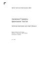
NASA Technical Memorandum 4442
Variational Trajectory
Optimization Tool Set
Technical Description and User’s Manual
Robert R. Bless, Eric M. Queen,
Michael D. Cavanaugh, Todd A. Wetzel
and Daniel D. Moerder
JULY 1993
NASA Technical Memorandum 4442
Variational Trajectory
Optimization Tool Set
Technical Description and User’s Manual
Robert R. Bless
Lockheed Engineering & Sciences Company
Hampton, Virginia
Eric M. Queen
Langley Research Center
Hampton, Virginia
Michael D. Cavanaugh
George Washington University
Hampton, Virginia
Todd A. Wetzel
Iowa State University
Ames, Iowa
Daniel D. Moerder
Langley Research Center
Hampton, Virginia
The use of trademarks or names of manufacturers in this
report is for accurate reporting and does not constitute an
ocial endorsement, either expressed or implied, of such
products or manufacturers by the National Aeronautics and
Space Administration.
Contents
List of Figures . . . . . . . . . . . . . . . . . . . . . . . . .
Abstract . . . . . . . . . . . . . . . . . . . . . . . . . . . .
Introduction . . . . . . . . . . . . . . . . . . . . . . . . . .
Background . . . . . . . . . . . . . . . . . . . . . . . . .
What Is the VTOTS? . . . . . . . . . . . . . . . . . . . . .
VTOTS Software . . . . . . . . . . . . . . . . . . . . . . .
Capabilities . . . . . . . . . . . . . . . . . . . . . . . . .
Purpose and Overview of Report . . . . . . . . . . . . . . . .
Symbols . . . . . . . . . . . . . . . . . . . . . . . . . . . .
Technical Description of Methods . . . . . . . . . . . . . . . . .
Generalized Optimal Control Problem . . . . . . . . . . . . . .
Finite-Element Method . . . . . . . . . . . . . . . . . . . .
Shooting Method . . . . . . . . . . . . . . . . . . . . . . .
Concluding Remarks . . . . . . . . . . . . . . . . . . . . . .
Appendix A|User's Manual . . . . . . . . . . . . . . . . . . .
Using MACSYMA for Problem Setup . . . . . . . . . . . . . .
The setup le . . . . . . . . . . . . . . . . . . . . . .
Variable names to avoid . . . . . . . . . . . . . . . . . .
Example setup le (problem.mac) . . . . . . . . . . . .
Creating the MATLAB plant module (plant.mex4) . . . .
Time Scaling . . . . . . . . . . . . . . . . . . . . . . . . .
The File Vtotsinfo.m . . . . . . . . . . . . . . . . . . . . .
Variables common to the nite-element and shooting algorithms
Finite-element variables . . . . . . . . . . . . . . . . . .
Shooting variables . . . . . . . . . . . . . . . . . . . .
Overview of Problem Setup . . . . . . . . . . . . . . . . . .
Solution Method Options . . . . . . . . . . . . . . . . . . .
Output . . . . . . . . . . . . . . . . . . . . . . . . . . .
Program Diagnostics . . . . . . . . . . . . . . . . . . . . .
Helpful Hints . . . . . . . . . . . . . . . . . . . . . . . . .
Detailed Example . . . . . . . . . . . . . . . . . . . . . . .
Appendix B|Additional Example Files . . . . . . . . . . . . . .
The Unconstrained Double Integrator . . . . . . . . . . . . . .
State-Constrained Double Integrator . . . . . . . . . . . . . .
Control-Constrained Problem . . . . . . . . . . . . . . . . . .
A Two-Stage-Rocket Problem . . . . . . . . . . . . . . . . .
Appendix C|Programmer File Reference List . . . . . . . . . . .
VTOTS Driver Subroutines . . . . . . . . . . . . . . . . . .
Finite-Element Method . . . . . . . . . . . . . . . . . . . .
Shooting Method . . . . . . . . . . . . . . . . . . . . . . .
References . . . . . . . . . . . . . . . . . . . . . . . . . . .
iii
.
.
.
.
.
.
.
.
.
.
.
.
.
.
.
.
.
.
.
.
.
.
.
.
.
.
.
.
.
.
.
.
.
.
.
.
.
.
.
.
.
.
.
.
.
.
.
.
.
.
.
.
.
.
.
.
.
.
.
.
.
.
.
.
.
.
.
.
.
.
.
.
.
.
.
.
.
.
.
.
.
.
.
.
.
.
.
.
.
.
.
.
.
.
.
.
.
.
.
.
.
.
.
.
.
.
.
.
.
.
.
.
.
.
.
.
.
.
.
.
.
.
.
.
.
.
.
.
.
.
.
.
.
.
.
.
.
.
.
.
.
.
.
.
.
.
.
.
.
.
.
.
.
.
.
.
.
.
.
.
.
.
.
.
.
.
.
.
.
.
.
.
.
.
.
.
.
.
.
.
.
.
.
.
.
.
.
.
.
.
.
.
.
.
.
.
.
.
.
.
.
.
.
.
.
.
.
.
.
.
.
.
.
.
.
.
.
.
.
.
.
.
.
.
.
.
.
.
.
.
.
.
.
.
.
.
.
.
.
.
.
.
.
.
.
.
.
.
.
.
.
.
.
.
.
.
.
.
.
iv
1
1
1
2
3
3
4
4
5
5
8
9
11
12
12
12
13
13
14
15
17
17
17
19
20
20
20
22
23
24
34
34
35
42
43
51
51
51
52
53
List of Figures
1. Discretized time line . . . . . . . . . . . . . . . . . . . . . . .
A1. Commands for creating plant.mex4 . . . . . . . . . . . . . . . .
A2. Flowchart of problem setup . . . . . . . . . . . . . . . . . . . .
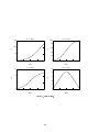
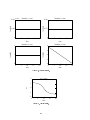
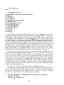
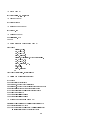
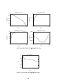
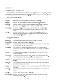
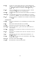
A3. State histories . . . . . . . . . . . . . . . . . . . . . . . . . .
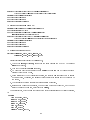
A4. Costate histories . . . . . . . . . . . . . . . . . . . . . . . . .
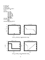
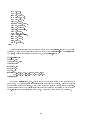
A5. Control history . . . . . . . . . . . . . . . . . . . . . . . . .
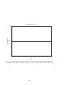
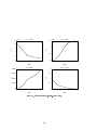
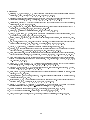
A6. Hamiltonian history (integral cost plus adjoined dynamics), measure of
global convergence of algorithm . . . . . . . . . . . . . . . . . .
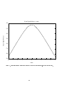
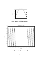
A7. Eigenvalues of the second partial of Hamiltonian with respect to control;
second-order sucient condition . . . . . . . . . . . . . . . . . .
B1. Unconstrained, double-integrator state histories . . . . . . . . . . .
B2. Unconstrained, double-integrator costate histories . . . . . . . . . .
B3. Unconstrained, double-integrator control history . . . . . . . . . . .
B4. Unconstrained, double-integrator Hamiltonian . . . . . . . . . . . .
B5. Unconstrained, double-integrator eigenvalues of Huu . . . . . . . . .
B6. Constrained, double-integrator state histories . . . . . . . . . . . .
B7. Constrained, double-integrator costate histories . . . . . . . . . . .
B8. Constrained, double-integrator control history . . . . . . . . . . . .
B9. Constrained, double-integrator Hamiltonian . . . . . . . . . . . . .
B10. Constrained, double-integrator eigenvalues of Huu . . . . . . . . . .
B11. Control-constrained problem state histories . . . . . . . . . . . . .
B12. Control-constrained problem costate histories . . . . . . . . . . . .
B13. Control-constrained problem control history . . . . . . . . . . . . .
B14. State histories for two-stage-rocket problem . . . . . . . . . . . . .
B15. Costate histories for two-stage-rocket problem . . . . . . . . . . . .
B16. Control history for two-stage-rocket problem . . . . . . . . . . . .
iv
.
.
.
.
.
.
.
.
.
.
.
.
.
.
.
.
.
.
. 8
16
21
30
31
31
. . . 32
.
.
.
.
.
.
.
.
.
.
.
.
.
.
.
.
.
.
.
.
.
.
.
.
.
.
.
.
.
.
.
.
.
.
.
.
.
.
.
.
.
.
.
.
.
.
.
.
.
.
.
33
36
36
37
37
38
40
40
41
41
42
44
45
45
49
50
50
Abstract
This report briey describes the algorithms that comprise the
Variational Trajectory Optimization Tool Set (VTOTS) package.
The VTOTS is a software package for solving nonlinear constrained
optimal control problems from a wide range of engineering and scientic disciplines. The VTOTS package was specically designed to
minimize the amount of user programming; in fact, for problems that
may be expressed in terms of analytical functions, the user needs only
to dene the problem in terms of symbolic variables. This version
of the VTOTS does not support tabular data; thus, problems must
be expressed in terms of analytical functions. The VTOTS package
consists of two methods for solving nonlinear optimal control problems: a time-domain, nite-element algorithm and a multiple shooting algorithm. These two algorithms, under the VTOTS package,
may be run independently or jointly. The nite-element algorithm
generates approximate solutions, whereas the shooting algorithm provides a more accurate solution to the optimization problem. A user's
manual, some examples with results, and a brief description of the
individual subroutines are included in this report.
Introduction
Background
The optimal control problem featured in this report is described as follows. Consider a
dynamical system dened by a nite-dimensional set of ordinary dierential equations, and
assume a nite-dimensional vector of time-varying control variables. The optimization problem
is to choose the control variables to satisfy the given boundary conditions while a given
performance index (or cost functional) is minimized (or maximized). Methods available for
the numerical solution of optimal control problems generally fall into two distinct categories:
direct and indirect. Direct methods, which involve parameter optimization, directly minimize
the performance index by varying the values of the parameters. Indirect methods, on the other
hand, minimize the performance index indirectly by satisfying rst-order necessary conditions
for optimality that are established from the calculus of variations.
The direct approach to the solution of optimal control problems requires parameterization of
the control and state time histories and results in a nonlinear programming problem to solve.
The choice of parameterization schemes is not unique, and success of the direct methods has
been achieved with Hermite polynomials (ref. 1), Chebyshev polynomials (refs. 2 and 3), singleterm Walsh series (ref. 4), and splines (ref. 5). After the parameterization scheme is chosen, a
parameter-optimization algorithm is used to determine the free parameters. These algorithms
are in common use today and include variable metric techniques or quasi-Newton methods
(ref. 6) and variations on gradient methods. Gradient methods (refs. 7 and 8) were developed to
surmount the \initial guess" diculty associated with other methods, such as Newton algorithms.
The gradient methods are characterized by iterative algorithms for improving estimates of the
state and control time histories. First-order gradient methods rapidly improve the state and
control histories during early iterations when suciently far from the optimal solution; however,
these methods exhibit only linear convergence close to the solution. Second-order gradient
methods provide quadratic convergence but are more sensitive to initial guesses. Conjugate
gradient methods exploit the approximately quadratic variation of the objective function near
the solution to accelerate convergence. Reference 9 contains a thorough description of the
gradient method and other algorithmic methods in optimal control.
Because the direct method is presented as a nonlinear programming problem, the solution
is much more dicult to obtain, especially from a software standpoint. Conversely, when the
indirect method satises the rst-order necessary conditions, the problem is converted into a
system of equations that form a multipoint boundary-value problem (MPBVP), which can be
solved with simpler root-nding techniques.
Analytical solutions to a MPBVP are generally unobtainable except for the simplest problems;
hence, numerical methods are usually employed. The two main methods for solving a nonlinear
MPBVP are shooting and quasi-linearization methods. Shooting methods (refs. 10 through 12)
are frequently used and can be described as follows. The dierential equations and the known
initial conditions are satised at each stage of the process, but the nal conditions are not
satised. A nominal solution is generated by guessing the missing initial conditions and
integrating the dierential equations forward to reduce the error in the nal conditions at each
iteration. Quasi-linearization methods (refs. 7 and 13) are used to choose nominal functions for
the states and costates that satisfy as many of the boundary conditions as possible. The control is
then found by using the optimality conditions. The system and costate equations are linearized
about the nominal values, and a succession of nonhomogeneous, linear, two-point boundaryvalue problems are solved to modify the solution until the desired accuracy is obtained. Other
indirect methods include the method of adjoints (ref. 14) and nite-element methods (ref. 15).
The system of equations in these methods is typically solved by Newton-Raphson (ref. 16) or
continuation algorithms (ref. 17).
A few of the commercially available programs for solving optimal control problems are
mentioned below. The rst two programs solve general MPBVP's, whereas the last two are
particularly designed to optimize ight-vehicle trajectories.
The Chebyshev Trajectory Optimization Program (CTOP) is useful in several practical
applications (ref. 2). This program solves problems directly and parameterizes the functions
using Chebyshev polynomials. Penalty functions enforce the equations of motion and path
constraints. The Nonlinear Programming for Direct Optimization of Trajectories (NPDOT)
package uses piecewise polynomials and collocation to satisfy the dierential equations. Results
presented in reference 1 show that the NPDOT runs more quickly than the CTOP does. Both
programs are generic optimization programs that are not limited to aerospace problems.
The Program to Optimize Simulated Trajectories (POST) targets and optimizes point-mass
trajectories for a powered or unpowered vehicle that operates near a rotating oblate planet
(ref. 18). The POST allows the solution of a wide range of ight problems that include
aircraft performance, orbital maneuvers, and injection into orbit. The user can select the
optimization variable, the dependent variables, and the independent variables from a list of more
than 400 program variables. The POST also operates on several computer systems. Another
useful program is Optimal Trajectories by Implicit Simulation (OTIS). The OTIS is a threedegree-of-freedom (point-mass) optimization program that includes a six-degree-of-freedom and
multiple-vehicle simulation (ref. 1). The user can simulate aircraft, missiles, reentry vehicles,
and hypervelocity vehicles. The methods used were chosen to improve speed, convergence, and
applicability of the OTIS over existing performance programs. Both the POST and the OTIS
are reliable and accurate programs, but they specically target aerospace applications.
What Is the VTOTS?
The VTOTS package is a set of optimal control algorithms, each based on a common, problemspecic, user setup and interface. The two methods for solving optimal control problems are a
2
nite-element and a shooting method. Each method uses a symbolic mathematics package to
organize the system equations and to calculate system Jacobians. The VTOTS package also
uses the nite-element algorithm to obtain initial estimates for the more accurate shooting code.
Combining the nite-element results with a shooting initial condition provides a fast solution
technique for nonlinear optimal control problems.
The VTOTS package was designed to minimize the user programming needed to solve optimal
control problems and still provide a quick, accurate solution procedure. Three software packages
that are used by the VTOTS are described in the next section.
VTOTS Software
The VTOTS optimal control algorithms use three computer languages:
1. MACSYMA MACSYMA is a symbolic mathematics package that computes analytical derivatives of mathematical expressions. A VTOTS preprocessor
was written in MACSYMA, a language developed by Symbolics, Inc., to
organize and calculate expressions needed by the VTOTS algorithms.
The preprocessor then translates these mathematical expressions into
FORTRAN.
2. FORTRAN
The result of the VTOTS preprocessor is a series of FORTRAN subroutines that are written to disk. Each subroutine is generated by the
MACSYMA algorithm.
3. MATLAB
MATLAB is a computer language that specializes in matrix manipulation and vector analysis. The VTOTS program and associated algorithms are written in MATLAB, a language developed by Mathworks,
Inc. The FORTRAN subroutines supplied by MACSYMA are compiled
into a single, problem-specic module using a MATLAB compiler. The
plant module is then accessed by MATLAB function les.
Capabilities
The VTOTS package provides solutions to a variety of optimal control problems with both
the nite-element and shooting algorithms. Both algorithms can solve nonlinear optimal control
problems with multiple-state or state-rate discontinuities. Also, the boundary conditions can
be any nonlinear function of the states. The nite-element algorithm, but not the shooting
algorithm, solves problems with control and/or state constraints. The number of control
constraints is arbitrary; however, it is assumed that the same number of constraints acts
over the entire tra jectory, and only one state constraint is active at a time. Furthermore,
for problems with state constraints, the control is assumed to be continuous across junction
points of constrained and unconstrained arcs. Assuming continuity of the control is tantamount
to saying that the Hamiltonian of the problem is regular; that is, a unique optimal control exists
for a given state and costate time history. The user should be aware of these assumptions and
carefully study solutions obtained from the VTOTS package, especially for constrained problems.
In general, the user should be aware that with the nite-element algorithm, or any discretization
algorithm, the output is only a candidate solution to an extremal.
For problems with control constraints, the user is not required to specify the switching
structure of the constraint; in other words, the user does not need to know or specify in the
problem setup when the constraints will be active or inactive. However, for problems with state
constraints, the user must know the order in which the constrained and unconstrained arcs occur.
Further, if the program has active control and state constraints, a switching structure must be
3
specied only for the state constraints. Details and examples of handling constrained optimal
control problems are presented in subsequent sections.
Finally, neither the nite-element algorithm nor the shooting algorithm handles optimal
control problems with singular arcs.
Purpose and Overview of Report
This report describes the nite-element and shooting algorithms and explains how to solve
optimal control problems with the VTOTS. The section \Technical Description of Methods"
denes an optimal control problem and provides a technical description of the nite-element
and shooting algorithms. A brief discussion of each algorithm and the VTOTS package is then
presented. \Concluding Remarks" summarizes the unique features of the VTOTS. Appendix A
is a user's manual for solving optimal control problems with the VTOTS and includes an example
and some helpful hints. Appendix B contains several additional example les and output for
problems that are solvable with the VTOTS. Finally, appendix C briey describes the VTOTS
MATLAB les.
Symbols
F
f
g
H
J
J1
k
L
M
m
N
n
q
S
tf
ti
u
V
x
^
x
x
x_
vector of right sides for state and costate equations
right side of dierential equations
state and control constraints
Hamiltonian
scalar performance index
scalar augmented-performance index
slack variable
integral portion of performance index
number of elements
number of controls
number of phases
number of states
order of state inequality constraint
state inequality constraints
nal time
time at ith event
control vector
vector containing states and costates
state vector
state vector at event points
state vector at midpoints
state time derivative vector
4
x
; 8
Abbreviations:
CTOP
I
MPBVP
NPDOT
OTIS
POST
VTOTS
state variation
costate variation
multiplier vector
time scales
costate vector
multiplier vector
vector of Lagrange multipliers
discrete portion of augmented performance index
discrete portion of performance index
vector of boundary condition expressions
Chebyshev Trajectory Optimization Program
identity matrix
multipoint boundary-value problem
Nonlinear Programming for Direct Optimization of Trajectories
Optimal Trajectories by Implicit Simulation
Program to Optimize Simulated Trajectories
Variational Trajectory Optimization Tool Set
Technical Description of Methods
In this section, a nonlinear constrained optimal control problem is dened. Then, a brief
description of a nite-element method and a shooting method is presented to solve the optimal
control problem. Further details of these methods are given in the cited references.
Generalized Optimal Control Problem
An optimal control problem is dened below. First, the notation is dened and the rst-order
necessary conditions for unconstrained problems are derived. Then, the inclusion of constraints
on the system is considered, and the additional conditions for optimality are dened.
Consider a system that is dened from initial time t0 to nal time tf by a set of n states x and
a set of m controls u. The states of the system are governed by a set of rst-order di erential
equations referred to as state equations. During the interval t0 to tf , discontinuities in the states
as well as in the state equations may occur at interior points (i.e., times between t0 and tf ).
These interior, initial, and nal points are referred to as events, and the intervals between events
are referred to as phases. The time of event i is denoted as ti , and the states and controls in
phase i are denoted as x(i) and u(i).
The optimal control problem of interest in this report is to choose a control history that
minimizes a performance index J and satises the state equations x_ (i) = f (i)[x(i); u(i)] and
boundary conditions. Elements of a performance index may be denoted with an integrand
L(i)[x(i); u(i)], which is continuous and dierentiable within each phase, and a discrete function
5
of the states and/or times at any of the events. A general class of such problems with N
phases involves choosing u(t) to minimize
J
=
i XN Z t i hx i u i i
h
x(1) (t1) ; x(1) (t2) ; x(2) (t2) ; x(2) (t3) ; : : : ; x(N ) (tN+1) ; t1; t2; : : : ; tN +1
h
i
+1
i
+
i=1 ti
L( )
;
()
()
dt
(1)
subject to the state equation constraints
x_ (i) = f (i) x(i); u(i)
h
(ti < t < ti+1 ; i = 1; 2; : : : ; N )
(2)
i=0
with boundary conditions specied as
x(1) (t1 ) ; x(1) (t2 ) ; x(2) (t2 ) ; x(2) (t3 ) ; : : :; x(N ) (tN +1) ; t1; t2; : : :; tN +1
(3)
With the introduction of Lagrange multiplier functions (t), referred to as costates, and
discrete Lagrange multipliers , an augmented performance index J1 may be dened as
J1 = + T
+
XZ
N
i=1
ti+1
ti
T
L(i) + (i)
h
i
f (i) 0 x_ (i) dt
(4)
For convenience, 8 and H are dened as
8 + T
(5)
and
T
H (i) L(i) + (i) f (i)
(i = 1; 2; : : :; N )
(6)
The rst-order necessary conditions for optimality are derived by requiring J1 to be stationary.
The conditions are (ref. 7)
h
i
(7)
@H (i)
@ x(i)
= 0Hx(i)
(8)
x_ (i) = f (i) x(i) ; u(i)
T
_ (i) = 0
@H (i)
= Hu(i) = 0
(
i
)
@u
where each equation holds for ti < t < ti+1 and i = 1; 2; : : :; N .
=0
(i01) (ti ) =
T
(9)
The boundary conditions are
(10)
@8
@ x 01) (ti )
T
@8
(i) (ti ) = 0 (i)
@ x (ti )
(i
and the transversality conditions are
@8
0 H (1) (t1) = 0
@t
1
6
(i = 2; 3; : : :; N + 1)
(11)
(i = 1; 2; : : :; N )
(12)
(13)
@
8+
i
@t
H
i01) (ti ) 0 H (i) (ti ) = 0
@
8 +
N +1
@t
( =2 3
(
H
i
;
;: : :;N
)
(14)
N ) (tN +1) = 0
(15)
(
The optimal control problem dened above is a nonlinear MPBVP. The solution to the
MPBVP yields a stationary point of 1, or a candidate optimal solution.
The problem can now be extended to include control and state inequality constraints on the
system. Control constraints (see a standard optimal control text, such as ref. 7, for details) are
dened as a function of the states and the control (where the control appears explicitly, but the
states may not) of the form
(16)
g (x u) 0
To solve this problem, the constraint g is adjoined to the cost function with a Lagrange multiplier
function ( ). This augmentation is equivalent to redening the Hamiltonian of the system
as
(17)
= + T f + T g
The necessary conditions in equations (7) through (15) remain unchanged when the new
denition of is used. However, the multiplier requires additional necessary conditions.
For a minimizing problem, the conditions are as follows: a multiplier of zero when the constraint
is not active (g 0) and a nonnegative multiplier when the constraint is active (g = 0).
Consider problems with state inequality constraints of the form S(x) 0. One of several
methods available to solve problems with state constraints is to take total time derivatives
of the constraint until the control appears explicitly; this method requires substitution of the
dierential equations for the state rates. If time derivatives are required for the control to
appear explicitly, then the constraint is referred to as a th-order state inequality constraint.
Now the th time derivative of the constraint plays the same role as the control constraint g(x u)
above. After a Lagrange multiplier function ( ) is introduced, the Hamiltonian is
J
;
t
H
H
L
H
<
q
q
q
;
t
H
= + T f + T
L
qS
q
dt
(18)
d
where the following statements apply:
1. The multiplier = 0 when the constraint is not violated (S 0).
2. The value q S q = 0 when the constraint is active (S = 0).
3. The multiplier 0 when the constraint is active if minimizing cost.
In addition to taking time derivatives of the constraint, tangency conditions must be met
at the point of entry onto a constrained arc. These conditions are that S and the rst ( 0 1)
time derivatives of S are zero at the beginning of a constrained arc. Also, the states must be
continuous at the beginning and end of each arc. These boundary conditions are placed in ;
because of these conditions, the user must dene the switching structure of the constrained
arc. Thus, the user must decide when the trajectory enters and leaves the constraint boundary,
because each independent arc of the trajectory is a new phase with corresponding boundary
conditions.
<
d
=dt
q
Without loss of generality, all constrained problems can be set up as minimizing problems with
the constraints dened as less than or equal to zero. The VTOTS also requires this constraint
format.
7
Finite-Element Method
The nite-element method converts the continuous-time necessary conditions into nonlinear
algebraic equations. The process for generating the algebraic equations is outlined below. Full
details of the method are described in reference 15.
For simplicity, the nite-element method is outlined for a one-phase problem, that is, one with
no internal events. To begin the derivation of the nite-element equations, the rst variation
of an augmented performance index is taken; the resulting expression is integrated by parts so
that no time derivatives of the states x or costates appear. Instead, one time derivative of the
variational states x and variational costates appears. This appearance identies the simple
choice of approximating functions. Next, shape functions, or approximating functions, for the
states, costates, and controls are chosen. With the expression that is developed for the rst
variation, the simplest possible shape functions are chosen for the states, costates, and controls,
namely, piecewise-constant functions.
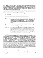
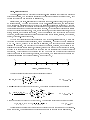
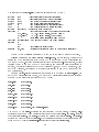
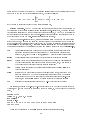
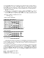
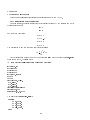
To begin the discretization scheme associated with this nite-element method, a time line
is broken into a series of equal segments, known as elements. The length of each element is
1t = (t1 0 t0)=M , where M is the number of elements. The endpoints of each element are
referred to as nodes. We will denote the values of the states, costates, and controls at the
element midpoints as barred symbols. Similarly, values at the nodes will be symbols with carets.
Figure 1 is an example of a time line that is broken into ve elements; only the state variables
are labeled. Nodal values at the beginning and end of a phase and at all midpoint values are
treated as unknowns for the states, costates, and controls. The remaining unknowns are the
discrete multipliers and the event times ti. (See appendix A.)
xˆ1
t0
xˆ2
x–1
x–2
x–3
x–4
x–5
t1
Figure 1. Discretized time line.
The state dierential equations that are discretized become
8 0x^ + x 0 1t f
>< 1 1 2 1
_ = f (x; u) ) 0 = > 0x i 0 12t fi + x i+1 0 12t fi+1
x
(i = 1; 2; : : : ; M 0 1)
: 0x 0 1t f + x^
M 2 M 2
where fi denotes the value of f at midpoint i. The costate dierential equations become
8 ^ 1t
>< 1 0 1 0 2 Hx1
@ H(x; ; u; ; )
_ = 0
) 0 = i 0 12t Hx 0 i+1 0 12t Hx +1
(i = 1; 2; : : :; M 0 1)
@x
>: 0 1t 0 ^
M 2 M 2
where H i denotes the value of H at midpoint i. The algebraic optimality condition becomes
i; u i; ; ) = 0
xi ; (i = 1; 2; : : :; M )
Hu(x; ; u; ; ) = 0 ) Hu(
The remaining equations involve the state and costate boundary conditions and the transversality conditions. The same number of equations as unknowns appears in this formulation.
i
i
8
Additional algebraic conditions are associated with control constraints. The nite-element
algorithm handles the control inequality constraints g(x; u) 0 by introducing a positive
function k2 , such that g + k2 = 0. The function k is referred to as a slack variable and
becomes an unknown. Note that when on the constraint, g = 0; therefore, k = 0. Additional
unknowns associated with state constraints are listed in appendi x A.
A nite-element method yields an approximate solution to the optimal control problem. From
numerical experience, the accuracy of the solution, or closeness to the exact answer, increases
quadratically with the number of elements (ref. 15); however, for a numerically accurate answer,
a shooting method is available.
Shooting Method
The VTOTS includes a shooting algorithm for solving the necessary conditions in equations (7) through (15). The solution technique converts the MPBVP for the Hamiltonian system
(eq. (6)), subject to equation (7) and boundary conditions (eqs. (10) through (12)), into an algebraic root-nding problem in the values taken on by x, , and t at the initial and terminal points
of the trajectory and at internal events. The procedure is accomplished by expressing terminal
values of x and (their values at the end of phases) as functions of initial values (their values at
the beginning of phases). This conversion is achieved by integrating the solution of the ordinary
dierential equations (eqs. (7) and (8)) from the initial values to the terminal conditions.
For simplicity, consider the case with no internal events, so that the boundary conditions of
the problem are
0
1
x0; xf = 0
(19)
0T +
Tf 0
where
@
@
+ T
@
0 T @@x
@ x0
@ xf
@ x0
f
=0
(20)
=0
(21)
x0 x (0) ; 0 (0)
xf
x
0 1
tf ; f
0 1
tf
The variables xf and f are evaluated as
xf = x0
+ 2
f = 0 0
2
Z 1
0
f (x; u
^)
Z 1
@H
0
@x
d
^ ) d
(x; ; u
2
= tf
2
= tf
(22)
(23)
where H is the Hamiltonian that is dened in equation (6) and is evaluated along x(t), (t),
and u^(t), and u^ is a root of
@H
^) = 0
(24)
(x; ; u
@u
which is obtained by numerical solution of Hu = 0 in terms of x and at each instant. The
result is that u^ appears as u^ (x; ) in the calculations. The partial derivatives u^ x and u^ are
01 (Hux)
u^ x = 0Huu
9
(25)
01 (Hu)
u^ = 0Huu
(26)
Z 1
2
F(V) d
Vf = V0 + 0
(29)
where Huu is assumed to have full rank.
The variable in equations (22) and (23) is a parameter that scales the dummy independent
variable ,
(0 1)
(27)
t = 2
In the implementation of the VTOTS shooting algorithm, is appended to x as an additional
state variable with
_ = 0
(28)
and is solved with boundary conditions appropriate to the free- or xed-time problem. The
costate that corresponds to is appended to and is evaluated at t = t f with the appropriate
modication of equation (23).
The x, , , and variables and their propagation expressions (eqs. (22), (23), and (28))
are concatenated to form the system
VT
=
FT
=
which satises the equation
h
h
xT ; ; T ; i
f T ; 0; 0HxT ; 02 H
0
i
1
9 V0; Vf = 0
(30)
where 9 is a concatenation of equations (19) through (21), reexpressed in components of V0
and Vf .
Equation (30) is solved by expressing Vf as Vf (V0) with equation (29) and employing a
Newton-Raphson iteration to obtain V0. The j th iteration is
01 h
i
d9
(V ) = (V ) 0
9 (V )
(31)
(j = 0; 1; : : :)
0 j+1
0
j
0
dV0 j
j
The value (V0)0, the initial guess for the iteration, is usually provided by boundary values from
a converged, nite-element run. For problems addressed to date with the VTOTS, these values
have proved to be suciently close to the shooting solution so that no line search was necessary
in equation (31).
The Jacobian matrix d9=dV0 in equation (31) is
d9
= @ 9 + @ 9 dVf
(32)
dV0
where
dVf
@ V0
Z
@ Vf dV0
1
F dV
= I + 2 ddV
d
(33)
dV0
dV0
0
The use of equations (32) and (33) to obtain d9=dV0, rather than the use of direct numerical
dierentiation with respect to V0, is motivated by concern for numerical stability in integrating
10
V( ).
When the plant states x contain dissipative eects, some eigenvalues of the adjoint
dynamics in equation (8) will have positive real parts. Direct numerical dierentiation of 9(V )
would require perturbation of V , an action that could excite modes corresponding to unstable
eigenvalues. This problem is avoided through the use of equations (32) and (33).
Although the shooting method is slower than the nite-element method, the shooting method
solution is as numerically accurate as the integrator used to propagate the state and costate
equations.
0
0
Concluding Remarks
This report provides a technical overview and a brief description of the algorithms that
comprise a new software package for solving optimal control problems. Although many excellent
programs are available for this purpose, the Variational Trajectory Optimization Tool Set
(VTOTS) oers some new features.
1. The VTOTS provides two algorithms based on indirect methods; most available programs
are based on direct methods.
2. The VTOTS provides a nite-element algorithm for approximate solutions and a shooting
algorithm for numerically accurate solutions.
3. An optimal control problem from any discipline may be solved when properly formatted;
however, this exibility requires a VTOTS user to supply application-specic code.
The appendixes contain a complete user's manual that includes a detailed example and helpful
hints. Additional examples, even those using very few elements in the nite-element algorithm,
show that a good approximation to a solution is possible. This approximation may be used
to start the shooting algorithm. Finally, a brief description of the VTOTS-MATLAB les is
included.
NASA Langley Research Center
Hampton, VA 23681-0001
April 19, 1993
11
Appendix A
User's Manual
This appendix describes how to set up, run, and solve optimal control problems with the
VTOTS. In particular, the development of three les that are needed to run VTOTS is described.
These les are a plant module plant.mex4, a name list le namcom.nml, and a MATLAB le
vtotsinfo.m.
The rst stage in using the VTOTS system is to set up the optimal control problem in a
MACSYMA-readable form; this step is the creation of a le that denes specic MACSYMA
variable names, equation lists, cost expressions, and lists of parameters that dene the problem.
The MACSYMA setup le and commands for producing the MATLAB-FORTRAN interface
are described in the next section. The section entitled \Time Scaling" discusses how and when
to scale the independent variable of the problem. The \Vtotsinfo.m" section describes the
user-supplied MATLAB le that is read in by the VTOTS. That section includes a discussion
of the initial guess vector that is required for the nite-element and shooting algorithms. An
overview of the steps required to set up the VTOTS les is provided in the \Overview of Problem
Setup" section. The solution methods available to the user are described in the section entitled
\Solution Method Options." The \Output" section describes the output that is available to the
user when a VTOTS run is successfully completed. Some program diagnostics and helpful hints
are provided. Finally, a detailed example of the use of the VTOTS to solve an optimal control
problem is presented.
Using MACSYMA for Problem Setup
The rst step in solving an optimal control problem with the VTOTS is to set up the problem
in MACSYMA-readable form. This process separates the dynamics, boundary conditions, and
performance index of an optimal control problem and assigns these expressions to MACSYMAspecic variables. A general problem statement for an optimal control problem was given
previously.
The setup le. The following list of MACSYMA variable names must be loaded into the
MACSYMA memory stack. These variables must be loaded into the le problem.mac. Standard
MACSYMA syntax must be followed when these expressions are set up. See the MACSYMA
Reference Manual (ref. 19) for details.
stlist
ctlist
phi
thi
ellist
delist
psilist
tsilist
glist
qlist
list of state variable names
list of control variable names
scalar cost expression that is a function of states at events only
scalar cost expression that is a function of time at events only
list of integral cost terms; corresponds to L in the performance index
list of dierential equations; corresponds to f in the problem statement
list of boundary conditions that are a function of states at events only;
each term in psilist will be zeroed in the solution of the problem
list of boundary conditions on time for each phase; may be empty
list of state and control inequality expressions
list dening the switching structure and the q th time derivative of a state
constraint
12
namcom
list of scalar FORTRAN variables for placement in the parameter name
list; useful for parameters that vary across a family of problems; for
example, an initial condition could be put in
and then changed
without having to rerun MACSYMA
namcom
namarray
\list of lists" of variables appearing in the name list that need to be
dimensioned in FORTRAN; variables are expressed in
with the
correct dimension; for example,
dimensions
a at (3), b at (4), f at (7);
is optional
namarray
namarray: [[a,3],[b,4],[f,7]];
namarray
phi
psilist
The variables
and
have a common convention for dening event conditions. In
these variables, a state name followed by two indices is used. The rst index denotes the phase
number, and the second denotes the initial or nal time of the phase, 1 for initial and 2 for nal.
delist glist
qlist
The variables
,
, and
are lists of sublists. They contain one sublist for each
phase. Refer to the section entitled \Additional Example Files" for further clarication.
Variable names to avoid. The following variables cause errors that may not be detectable
by the MACSYMA preprocessor. In the following, # denotes a number and * denotes a wild
card.
c#
d#
e#
emq*
MACSYMA command line variable storage
MACSYMA display line variable storage
MACSYMA internal variable sequence
variable-name string reserved by VTOTS
sin cos log
exp
ijklm n
thyme
thi
The user must avoid the variables
,
,
, and
because these strings are treated as
the corresponding function names. Also, the user must avoid using the tangent function in the
setup le because MACSYMA does not successfully convert this function to FORTRAN. The
user is responsible for ensuring that each variable name used in the MACSYMA problem setup
does not begin with the letters , , , , , or because these letters are reserved for integers in
FORTRAN. Do not use
as a variable except in
and
. Also, any MACSYMA
keyword that is used as a variable name leads to unpredictable results. The user should always
check the MACSYMA output for error messages.
tsilist
(problem.mac).
Example setup le
This example will help the reader understand how
the MACSYMA setup le is dened. A complete optimal control problem example is presented
in the section entitled \A Detailed Example."
u
Consider this linear-quadratic optimal control problem: nd (t) to minimize the scalar
performance index J, where
Z 1h
i
2 (t) + 2 (t) dt
J=
0
subject to
with boundary conditions
u
x
x_ (t) = x (t) + u(t)
x(0) = 0
x(1) = 1
13
The following le (problem.mac) loads this problem into MACSYMA:
stlist:
ctlist:
glist:
qlist:
phi:
thi:
ellist:
psilist:
[x];
/*defines the state variable names*/
[u];
/*defines the control variable names*/
[[]];
/*no control constraints specified*/
[[]];
/*no state constraints specified*/
0;
/*no discrete cost on states defined*/
0;
/*no discrete cost on times defined*/
[x^2+u^2]; /*quadratic cost function*/
[
/*Notice the indices for boundary conditions*/
x(1,1)-x0,
/* (1,1) - 1st phase, initial time */
x(1,2)-xf
/* (1,2) - 1st phase, final time */
];
/*The same index scheme is used in phi*/
tsilist: [thyme(1)-1]; /*(1) - final time of the first phase*/
delist: [[
x+u
]];
/*differential equations */
namcom: [x0,xf];
/*these variables are found in the FORTRAN namelist*/
The MACSYMA comments (delimited by /* and */) on the right do not need to appear.
Creating the
plant module
In this section, a listing of le
names and UNIX commands is given to show how to use the MACSYMA preprocessor and
how the MACSYMA-produced les are compiled into a single problem-specic module. Several
versions of MACSYMA and FORTRAN are available, and these vary from one machine to
another. The existing versions of MACSYMA (version 417.100), FORTRAN (version 1.4), and
MATLAB (version 3.5i) described in this report are specic to Sun SPARCstation IPC and
IPX workstations.
After the problem-specic information has been set up in a le such as problem.mac, the
MACSYMA preprocessor can be run. The MACSYMA preprocessor consists of the following
nine MACSYMA script les that create FORTRAN les:
allell.mac
allf.mac
allg.mac
allq.mac
allphi.mac
allthi.mac
allpsi.mac
alltsi.mac
plant.mac
MATLAB
(plant.mex4).
creates allell.f
creates allf.f
creates allg.f
creates allq.f
creates allphi.f
creates allthi.f
creates allpsi.f
creates alltsi.f
creates plant.f and namcom.nml
The FORTRAN le allell.f evaluates the cost integrand L for all phases. Similarly, allf.f
evaluates the right side of the dierential equations for all phases; allg.f and allq.f evaluate
the constraints; allphi.f and allthi.f evaluate the discrete cost terms; allpsi.f and alltsi.f
evaluate the boundary conditions; plant.f is the master routine that coordinates calls to the
other FORTRAN les; and namcom.nml contains the variables in namcom.
14
One additional le, plantg.f, is required to construct the plant module. This le is supplied
and does not require changes by the user. The le plantg.f is a gateway le to pass information
between the FORTRAN routines and MATLAB.
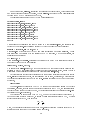
The commands for running the MACSYMA preprocessor are:
batch("problem.mac");
gentranin("plant.mac",["plant.f"]);
gentranin("allf.mac",["allf.f"]);
gentranin("allell.mac",["allell.f"]);
gentranin("allphi.mac",["allphi.f"]);
gentranin("allthi.mac",["allthi.f"]);
gentranin("allg.mac",["allg.f"]);
gentranin("allq.mac",["allq.f"]);
gentranin("allpsi.mac",["allpsi.f"]);
gentranin("alltsi.mac",["alltsi.f"]);
quit();
This sequence of commands can also be placed in a le (batchle.mac, for example) and
batched at the system-level command prompt by typing the following batch command:
macsyma < batchfile.mac >! std.out &
where std.out will contain MACSYMA run time information and error messages. These
les must then be compiled with the system FORTRAN compiler. On the Sun systems, the
commands are as follows:
f77 -c all*.f &
Then the plant.f and plantg.f les must be compiled with a MATLAB compiler and linked to
the other object code with the command
fmex plant.f plantg.f all*.o
The result is the plant.mex4 le, which can be moved to a convenient working directory and
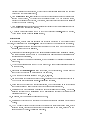
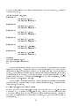
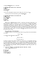
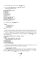
accessed by MATLAB routines in much the same way that functions are called. Figure A1 shows
a summary of the commands for creating the plant module plant.mex4.
Any plant module that is acceptable for use with the shooting algorithm will also work for the
nite-element algorithm; however, the converse may not be true. For example, a plant module
that includes constraints will work with the nite-element algorithm but not with the shooting
algorithm.
Time Scaling
The nite-element algorithm in the VTOTS does not require special scaling of the time
parameter. However, in order to run the shooting algorithm in the VTOTS, the user must scale
the time of each phase to a length of one. This procedure requires the conversion of free-time
problems to xed-time problems.
The variable is dened such that = t=tf , where t is the independent variable and tf
is the nal time (possibly unknown). Because t varies monotonically from 0 to tf , varies
monotonically from 0 to 1. Also note that
dx dx
= tf
d
dt
Thus, the dierential equations for any xed nal-time problem can be scaled from 0 to 1 by
multiplying each equation by the desired known nal time.
15
files:
problem.mac
allell.mac
allf.mac
allg.mac
allq.mac
allphi.mac
allthi.mac
allpsi.mac
alltsi.mac
plant.mac
(USER supplied)
(VTOTS supplied)
"
"
"
"
"
"
"
"
MACSYMA Environment
commands:
files:
batch("problem.mac");
gentranin("plant.mac",["plant.f"]);
gentranin("allf.mac",["allf.f"]);
gentranin("allell.mac",["allell.f"]);
gentranin("allphi.mac",["allphi.f"]);
gentranin("allthi.mac",["allthi.f"]);
gentranin("allg.mac",["allg.f"]);
gentranin("allq.mac",["allq.f"]);
gentranin("allpsi.mac",["allpsi.f"]);
gentranin("alltsi.mac",["alltsi.f"]);
quit();
plantg.f
plant.f
allf.f
allell.f
allphi.f
allthi.f
allg.f
allq.f
allpsi.f
alltsi.f
(VTOTS supplied)
(MACSYMA generated)
"
"
"
"
"
"
"
"
FORTRAN/MATLAB Environment
commands:
file:
f77 -c all*.f &
fmex plant.f plantg.f all*.o
plant.mex4
(used by VTOTS for problem specific information)
Figure A1. Commands for creating plant.mex4.
16
This method can be used even if the nal time is not known a priori. For a free nal-time
problem, dene an extra state, for example , to be solved by the system. The dierential
equation for is
_ = 0
so that is a constant. Its value is equal to the nal time (as yet unknown). In this case, to
prevent the time scale from becoming negative, set = t=tf = t= 2 . Now,
dx
dx
= 2
d
dt
Therefore, all the dierential equations are multiplied by 2 .
Similarly, the VTOTS can also solve nonautonomous problems. In this instance, the time
t becomes a state, with the additional boundary condition that this new state has an initial
condition of 0; the corresponding dierential equation is t_ = 1.
Multiphase problems can be handled by a straightforward extension of this technique.
Examples of time scaling are given in the \Additional Examples" section.
The File Vtotsinfo.m
In addition to the les namcom.nml and plant.mex4 created in the MACSYMA environment, the user must supply a MATLAB le called vtotsinfo.m. Because the VTOTS uses an
iterative method to solve MPBVP's, an initial guess is required. The le vtotsinfo.m stores
this initial guess with several other optional variables.
Some variables are common to both algorithms and some are specic to either the niteelement or the shooting algorithm. All the variables are discussed below.
Variables common to the nite-element and shooting algorithms. The following
variables may be dened in vtotsinfo.m; if not dened, they are not used:
prob name
timestate
scale
comment about the current problem; placed in single quotes
integer between 1 and number of states in problem, which corresponds
to position of time state; timestate dened only for plotting purposes;
dening timestate automatically scales the x-axis of the plots to the
correct values of the independent variable
matrix of scaling factors n by nph, where n is the number of states plus
costates and nph is the number of phases; each row of the matrix scales
the states and costates in the corresponding phase; the i, j element of
scale multiplies the ith state in the j th phase; for a problem that has
been nondimensionalized, scale will dimensionalize the problem; as an
example, see the section entitled \A Two-Stage-Rocket Problem" in
appendix B
Finite-element variables. The following variables are dened by the user in vtotsinfo.m
if the nite-element algorithm is run:
jbcv
yin
vector of number of elements in each phase; vector length is equal to
number of phases; jbcv determines the mesh density of the solution in
each phase; jbcv 1; this variable is required
vector of initial estimates for all unknowns; size and order of the initial
guess are dened below; this variable is required
17
converge
variable that denes the convergence criterion; default value is 1 2 1009 ;
sometimes useful to raise this convergence value if the code approaches a
solution but does not reach it; raising convergence value allows the user to
look at the answer before full convergence is reached to see if the solution
is being approached or not; this variable is optional
In order to use the nite-element method, estimates must be provided for all unknowns.
Consider a single-phase problem. A set of unknowns occurs at the midpoint of each element
(denoted by z) and also at the beginning and end of each phase z^. Each set of unknowns
consists of, in the following order, the states ( x1 ; : : : ; xn ), the costates ( 1 ; : : : ; n), the controls
(u1; : : : ; um), the multipliers for each control constraint ( 1; : : : ; np ), the slack variables for
each control constraint ( k1; : : : ; knp), and the multipliers for the state constraints ( 1 ; : : : ; nq ).
There may not be any constraints; therefore, no multipliers or slack variables are re quired.
After these estimates have been assembled, several more estimates are added to the end. These
estimates correspond to the discrete Lagrange multipliers that adjoin the boundary conditions
held in and to the discrete multipliers t that adjoin the boundary conditions in tsi. Finally,
an estimate for the nal time is made after the multiplier estimates.
For brevity, the set of unknowns for a problem with three states, two controls, one control
constraint, one state constraint, four state boundary conditions, and one time boundary
condition is
z = (x1; x2 ; x3 ; 1 ; 2 ; 3 ; u1 ; u2 ; 1 ; k1 ; 1 )
and the format of the initial estimates for jbcv = 5 is
0
z^1 ; z1 ; z2 ; z3; z4 ; z5 ; z^2 ; 1 ; 2 ; 3 ; 4 ; t1 ;
t1
1
A general formula can be dened for the size of the initial estimate le. Name the number of
states nx, the number of controls nu, the number of control constraints np, the number of state
constraints nq , the number of state boundary conditions (length of psi) mbc, the number of time
boundary conditions (length of tsilist) tbc, and the number of phases nph. Also, the variable
jbcv denes the number of elements per phase. The formula for determining the number of
initial guesses for single-phase problems is
(2nx + nu + 2np + nq ) (jbcv + 2) + mbc + tbc + 1
For example, a single-phase problem with three states, two controls, one control constraint,
zero state constraints, four state boundary conditions, one time boundary condition, and ve
elements would require an initial guess le of length (3 + 3 + 2 + 2)(5 + 2) + 4 + 1 + 1 = 76.
For multiple-phase problems there is an obvious extension to this formula. Unknowns occur
at the midpoint of the elements in each phase and at the endpoints of each phase. Two coincident
nodes appear at the juncture of phases. Although these nodes occur at the same instant, the
values of the variables (states, costates, and controls) may be di erent. In fact, this discontinuity
in one or more variables often requires introduction of the additional phases. The assembly of
the initial guess vector is similar to the single-phase process. Sets of unknowns for the rst phase
are assembled as described above for the single-phase problem. Next, before the values of are
added, sets of unknowns are added for the second and subsequent phases. At the juncture of
phases, the sets of unknowns may have identical values. When all phases have been assembled,
18
one for each boundary condition in and tsi and estimates for the nal times of each phase
are added to the end of the initial estimate vector. The general formula
2
nph
X
4
(2nx + nu + 2np + nq )
i=1
3
jbcv (i) + 2nph5 + mbc + tbc + nph
may be used to calculate the length of the initial estimate le.
Shooting variables. The VTOTS provides a shooting algorithm that may be run directly or
automatically (without user interface) after a successful nite -element run. The setup outlined
in this section describes how to run the shooting algorithm directly. (The VTOTS initializes the
shooting startup automatically when the nite-element/shooting method is operating so that no
additional setup beyond the nite-element initialization is required.)
As with the nite-element method, starting estimates must be provided for all shooting
method unknowns, which are the state and costate values at the beginning of each phase and
at any user-specied interior phase points (nodes). In addition, this method requires Lagrange
multipliers and a control estimate. A summary of these estimates and the variables that specify
the number and frequency of nodes is shown below and must be included in the le vtotsinfo.m.
yin
utrial
nnode
ynu
time
err
initial estimates for each phase and node; this column vector must contain the
states and costates of the rst phase P
followed by the states and costates of the
rst node, etc.; length of yin = 2nx[ (nnode) + nph]; this variable is required
control estimate for the system at the initial time; this variable is required
column vector that contains number of nodes in each phase; the rst element in
the vector species the number of nodes in the rst phase, etc.; a 0 is needed if
the phase does not contain nodes; this variable is required
column vector containing the Lagrange multipliers; length of ynu=mbc; this
variable is required
matrix in which each column holds node times for each phase, including a 0 to
start the phase and a 1 to end it; shorter columns (fewer nodes in a particular
phase) must be padded with 0's to make the matrix square; for a single-phase
problem, the vector time must be a column vector; this variable is required
species the integrator error; default is 1 2 1006; this variable is optional
For example, consider a two-state, two-phase problem with two nodes in the rst phase (at
times 0.2 and 0.6) and one node in the second phase (at time 0.5). Three boundary conditions
exist.
nnode = [2 1];
time = [0 .2 .6 1; 0 .5 1 0]';
err = 1e-6;
utrial = -.5;
yin = [ 1 2 3 4 5 6 7 8 9 10 11 12 13 14 15 16 17 18 19 20];
ynu = [1 2 3];
Notice that the trailing 0 in the time variable makes the matrix rectangular.
19
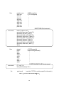
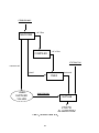
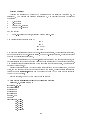
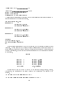
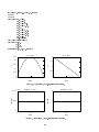
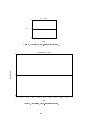
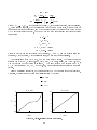
Overview of Problem Setup
The problem-setup procedure is illustrated in gure A2. Three les in this procedure are
provided by the user: problem.mac, namcom.nml, and vtotsinfo.m. The MACSYMA le,
in this case problem.mac, can have any name; however, the other two les must be named
namcom.nml and vtotsinfo.m. The rst step is to process the MACSYMA le as described
in the section entitled \Using MACSYMA for Problem Setup" to produce the les plant.f and
namcom.nml and eight other FORTRAN les. At this point, the name list le namcom.nml
has a list of parameters with no values. The user must edit this le and input the parameter
values. Next, the all*.f les should be compiled to form object les. The object les, the
plant.f le, and the plantg.f le are combined into a le called plant.mex4 through the use
of the MATLAB fmex utility. At this point, the command vtots in MATLAB causes VTOTS
to access the les plant.mex4, vtotsinfo.m, and namcom.nml. The user is prompted for
several options, which are discussed in the next section.
Solution Method Options
After the plant.mex4, namcom.nml, and vtotsinfo.m les are created, the user is ready
to start MATLAB and run the VTOTS by typing in vtots at the MATLAB prompt. A menu
appears that lists four solution method options. The user can choose the nite-element algorithm,
the shooting algorithm, or the nite-element algorithm followed by the shooting algorithm. The
fourth option is to exit the program, a useful choice if the name list le is not set properly or if
the initial estimate le is not the proper length. The word READY appears next to each option if
the initial estimate is the proper size. Choosing an option without a READY results in errors.
When the option for a nite-element algorithm is chosen, the user must decide between three
dierent solution methods to solve the algebraic equations. The user is prompted to choose
between a continuation method, MATLAB's fsolve algorithm (ref. 20), and a Newton method.
The continuation method is a simple type of homotopy described in reference 21. This option
is the most robust of the three methods (that is, it allows for the least accurate initial estimate
and still nds a solution), but it is also the slowest. After the continuation method is completed,
the Newton method is automatically called to obtain the solution. In certain cases, the integrator
for the continuation method is interrupted and gives an error message like
Singularity likely at t=0.456
The Newton method is called at this time and may converge on the solution; in such a case, the
message can be ignored.
The fsolve algorithm in MATLAB is a Newton method with a line-searching algorithm. The
fsolve algorithm is generally not as robust as the continuation method, but it does run faster.
The Newton method is the fastest of the three solution methods, but it requires the best
initial estimate. Generally, the Newton method should be attempted rst. If the program does
not converge, then either improve the initial estimate or try another method.
The shooting algorithm runs only a Newton method. In general, a nite-element solution
should be obtained before the shooting algorithm is attempted.
Output
After a successful nite-element run is executed, the user is prompted to save a variable called
yout. This variable is the same length as the user-supplied yin and contains the converged values
of the solution vector. To save this variable, use the command
save yout.dat yout /ascii
20
PROBLEM.MAC
all*.f files
MACSYMA
all*.o files
COMPILER
VTOTSINFO.M
namcom.nml
plant.f
plant.mex4
FMEX
USERSUPPLIED
VALUES
NAMCOM.NML
MATLAB
VTOTS
ALGORITHM
Figure A2. Flowchart of problem setup.
21
After completion of a nite-element solution, the user is always prompted to run another
problem with a dierent number of elements. The number of elements is usually increased to
obtain better accuracy, but the number of elements may be decreased. The user must input the
number of elements as a vector of a length that corresponds to the number of phases. When the
number of elements is increased (or decreased), code convergence is not guaranteed.
After completion of all nite-element or shooting runs, the program stores a matrix of values
in yall. This matrix is used for plotting, and it can be saved in the same way as yout, except
the user is not prompted to do so. The save command may be evoked after completion of the
plotting. The matrix yall contains the following columns of data: the time, the states, the
costates, the controls, the Hamiltonian, and the eigenvalues of the second partial derivative of
the Hamiltonian with respect to the controls. Because the Hamiltonian is constant for each phase
at the exact solution, the value of the Hamiltonian should be on the order of 1 2 1005 for the
shooting code, which uses an integrator with an error tolerance of 1 2 100 6 . The nite-element
algorithm is not as accurate unless the number of elements ( jbcv) is large. The eigenvalues
are important because they serve as a second-order necessary condition for a minimum or
maximum. The eigenvalues should be positive everywhere for a minimization problem and
negative everywhere for a maximization problem. Although the multipliers for the constraints
are not available in yall, these values are available in the vector yout.
The plotter routine may be called directly by the user if yall is saved. To call the plotter,
enter
plotter(nx,nu,yall)
at the MATLAB prompt. Each of these arguments should be in the workspace after a successful
run by either the nite-element or the shooting algorithm. Type help plotter for more
information.
Program Diagnostics
The following list shows some potential errors that can occur:
1. Common MACSYMA mistakes are
a. Use of an equal sign (=) instead of a colon (:).
b. Not ending a line with a semicolon (;), the result of which is usually a MACSYMA
error message stating that some variable is not an Infix operator.
c. Use of wrong number of brackets when dening MACSYMA variables. The variables
delist, glist, and qlist are \lists of lists" that require an extra set of brackets. Incorrect
number of brackets usually results in the message part fell off end.
d. Failure to compile, an indication of a mistake in the MACSYMA setup le.
2. Segmentation violation during a call to plant.mex4 is caused by a mistake in the
MACSYMA setup le.
3. No READY light by any of the solution options (except (4) Exit Program) indicates that
the initial estimate is not the correct length. Choosing the desired option should point to
the discrepancy.
4. Failure to provide values for the name list can produce strange results. (These values are
held in the le namcom.nml.)
5. A warning that a matrix is singular or badly scaled, given during a Newton method, means
that the Jacobian matrix is singular and cannot be inverted by MATLAB. In this case,
either the initial estimate leads to a singular matrix, the problem is poorly dened, or the
22
problem is singular at the solution. Fixing this problem requires remodeling the problem
or changing the initial estimate le.
6. A no converge in unod.m indicates that one of the control values during an interpolation
routine was not found. This condition is generally caused by a bad solution vector,
although convergence was obtained. Commonly, a state or control that is an angle assumes
a value in the wrong quadrant.
7. A no converge during a shooting run generally indicates that the initial estimate provided
by the user is too far from the solution.
8. A warning during compilation that a do loop is not executed in
This warning occurs whenever tsilist is empty.
alltsi.f
may be ignored.
Helpful Hints
In this section, helpful hints are suggested for obtaining a solution to an optimal control
problem. It is assumed that the plant.mex4 le is bug free and the name list le is complete.
1. A nite-element solution is almost always easier to obtain than a shooting solution;
therefore, start with nite elements.
2. When using nite elements, start with a small number of elements and increase; in general,
the initial estimate does not need to be as accurate for a small number of elements as for
larger numbers of elements.
3. When increasing the number of elements, it is not necessary to increase the elements in
each phase.
4. Avoid the use of numbers in the MACSYMA setup le. Dene these constants as variables
in the name list.
5. Make sure that namcom.nml is lled in properly, in double precision. A name list that
is not lled in could lead to a singularity in the Jacobian.
6. Avoid the use of variables starting with i, j, k, l, m, or n.
7. See the example in the section entitled \State-Constrained Double Integrator" for tips on
how to get switching structure for state-constrained problems.
8. When solving a problem with control constraints, do not choose zero as an initial guess
for the multiplier and slack variable; this choice causes a singular matrix.
9. Remember that all constrained problems must be minimization problems. Any maximization problem can be transformed into a minimization problem by multiplying the
performance index by 01.
10. In general, avoid an estimate of zero for unknowns.
11. Remember to list all known continuity conditions on states for problems with multiple
phases.
12. VTOTS cannot directly handle boundary conditions that contain states and time. If this
situation occurs, introduce another state that corresponds to the time, as shown in the
section entitled \Control-Constrained Problem."
23
Detailed Example
Consider the transfer of a particle to a rectilinear path as described in section 2.4 of
reference 7. The particle has constant acceleration a. The problem is dened in terms of
four states
x
y
u
v
x-coordinate
y -coordinate
velocity in x-direction
velocity in y -direction
and one control
angle-of-acceleration vector, measured positive from x-axis
The dierential equations are given by
x_ = u
y_ = v
u_ = a cos v_ = a sin The goal is to maximize the velocity in the x-direction after 20 sec. All states are initially zero,
and the nal velocity in the y -direction is zero. The nal y -coordinate is 100. There is no integral
cost and no constraints are imposed.
In order to demonstrate both the nite-element algorithm and the shooting algorithm, the
problem is scaled so that the phase has a duration of one (as required by the shooting algorithm).
The dierential equations are multiplied by the nal time to achieve the scaling. (See the section
entitled \Time Scaling.")
Several constants are used in this problem: the magnitude of the acceleration a, the nal
time, and the specied initial and nal conditions on the states. These constants are assigned
values in the le namcom.nml and can be changed between VTOTS runs without repeating
the MACSYMA process.
For this problem, the MACSYMA input le is as follows:
/* This is the fixed-time trajectory optimization problem
Section 2.4, Bryson and Ho */
stlist:[x,y,u,v];
ctlist:[beta];
glist:[[]];
qlist:[[]];
ellist:[0];
phi:u(1,2);
thi:0;
psilist:[x(1,1)-x0,
y(1,1)-y0,
u(1,1)-u0,
v(1,1)-v0,
y(1,2)-yf,
v(1,2)-vf];
24
tsilist:[thyme(1)-1];
delist:[[tim*u,tim*v,a*tim*cos(beta),a*tim*sin(beta)]];
namcom:[x0,y0,u0,v0,yf,vf,a,tim];
The name list le namcom.nml is
$namcom
X0 = 0.0d+00,
Y0 = 0.0d+00,
U0 = 0.0d+00,
V0 = 0.0d+00,
YF = 100.0d+00,
VF = 0.0d+00,
A = 1.12397d+00,
TIM = 20.0d+00,
$end
The name list starts with a dollar sign in the second column, and no data are entered in the
rst column. The MACSYMA scripts produce this le with the variable names but without the
values.
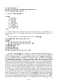
To run the problem, an initial guess must be supplied in vtotsinfo.m:
prob name='BHO-FIX - B&H Fixed time prob:';
jbcv=[5];
tab=[0.0 0.0 0.0 0.0 0.0 1.0 1.0 1.0 1.0 0.1;
1.0 100.0 100.0 10.0 0.0 1.0 1.0 1.0 1.0 0.1];
t=[0;.1;.3;.5;.7;.9;1.0];
yin=table1(tab,t);
yin=reshape(yin',63,1);
yin=[yin;ones(7,1);1.0];
scale=[20.0 1.0 1.0 1.0 1.0 1.0 1.0 1.0 1.0];
The rst line of vtotsinfo.m gives a comment that is displayed when the problem is run. This
comment is an optional declaration by the user. The second line denes the number of elements
in the rst nite-element run. This variable must be dened if the nite-element algorithm is
used. The user has the option of increasing or decreasing jbcv if the rst run is successful.
The next four lines demonstrate the ability of the MATLAB table1 function to create an initial
guess from linear interpolation. The matrix tab consists of 2 rows and 10 columns. The rst
column is an independent variable that starts at 0 and ends at 1. The next nine columns are
(in order) estimates at the states (four columns), estimates at the costates (four columns), and
estimates at the control (one column). In this example, only crude estimates for the beginning
and ending values of the variables are made, and table1 draws straight lines between them. For
example, in the third column of tab, the estimated value of the second state y is 0 at t = 0
and 100 at t = 1. The next variable is the column vector t. This variable denes the location
on the discretized time line where the estimates are needed. Recall that estimates are needed
at the endpoints of the phase and at the midpoints of the elements (g. 1). Next, the initial
guess of the solution is put in a column vector with the reshape command. Finally, estimates
for the discrete multipliers and time are added. Because psilist has a length of six and tsilist
has a length of one, seven estimates of 1 for the discrete multipliers are given. Also, because
the problem has been scaled to run from 0 to 1, the estimate for the nal time is 1. Finally,
25
the variable scale scales the output quantities. (See the section entitled \Variables Common to
the Finite-Element and Shooting Algorithms.") Because only the time line is scaled, the rst
number is 20.0 (the actual nal time) and the next 8 values (states and costates) are 1.0 (because
these were not scaled). Another example of the use of scale is given in the section entitled \A
Two-Stage-Rocket Problem."
Running the MACSYMA commands in gure A1 creates the plant.mex4 le. After the
plant les plant.mex4, vtotsinfo.m, and namcom.nml are created, VTOTS is ready to run.
After the user enters MATLAB, typing vtots at the MATLAB prompt returns the following:
Variational Trajectory Optimization Tool SET
VTOTS - v. 2.0
PROBLEM SPECIFIC INFORMATION
BHO-FIX - B&H Fixed time prob:
------------------------------------------------Number of states ...................... nx = 4
Number of controls .................... nu = 1
Number of control constraints ......... np = 0
Max. No. of active state constraints .. nq = 0
Number of state b.c`s ................. mbc = 6
Number of time b.c`s .................. tbc = 1
Number of phases ...................... nph = 1
Number of elements in phase number 1... jbcv(1) = 5
------------------------------------------------METHOD SELECTION
------------------------------------------------(1) Finite Elements .................. READY
(2) Shooting ......................... ----(3) F/E - Shooting ................... READY
(4) Exit Program ..................... READY
------------------------------------------------INPUT SELECTION ......................>>
The comment line is displayed and is followed by a brief summary of the important parameters
for this problem. Next, a list of options appears with a READY message indicating the options
that can be selected. Because the dierent methods require dierent initial guess forms, not all
methods are available at once.
In this example, the most powerful option for solving unconstrained optimal control problems
is demonstrated. Starting from the initial guess dened in vtotsinfo.m, the nite-element
algorithm is successfully run. Initial estimates can then be generated for the shooting algorithm
to produce an essentially exact answer to the problem. The nite-element/shooting option is
method 3 and is selected by typing 3 <cr> at the prompt. This selection leads to the following
message:
Enter 1 to run a continuation method
Enter 2 to run fsolve
otherwise <cr> to run a Newton method
26
Hitting a carriage return at this prompt begins execution of the Newton method. A sample of
the execution follows.
the initial error is 8.14201
step size = 1
the error is 3.66657
the iteration number is 1
step size = 1
step size = 1
step size = 1
step size = 1
step size = 1
the error is 0.508319
the iteration number is 2
the error is 0.220737
the iteration number is 3
the error is 0.0100028
the iteration number is 4
the error is 7.62849e-06
the iteration number is 5
the error is 2.0227e-12
the iteration number is 6
CONVERGED
Total run time is 20.5638
Now is your chance to save yout
K>>
The given initial estimate converged with the Newton method in six iterations and required
20.5638 sec of run time. The step size listed in the left column refers to the Newton method
line search step size. If the error is not reduced with the current step size , then the step size is
reduced. The step size is continually reduced until the error improves (decreases). In this case,
all iterations improved the error. Convergence is obtained when the error is less than 1 2 1009,
unless another value is set by the user in vtotsinfo.m with the variable converge. (See the
section entitled \Finite-Element Variables.")
The output after a problem converges should be saved because many successful initial estimate
les are generated by slight changes to output les from similar problems. A descriptive name
is also helpful. For example,
K>> save bhofix5.dat yout /ascii /double
saves the output in the le bhox5.dat (named for the Bryson and Ho xed-time problem
with jbcv = 5). The format is double-precision ascii. Usually, a good procedure is to start
with a small value for jbcv and build up until the desired resolution is reached. After saving
the output, type return <cr> at the K prompt to continue. Next, the code gives the option of
changing jbcv.
27
Change JBCV? y or n ..................>> y
INPUT JBCV ...........................>> [10]
Enter 1 to run a continuation method
Enter 2 to run fsolve
otherwise <cr> to run a Newton method
A carriage return here restarts the program, with an initial estimate automatically generated by
linear interpolation of the preceding solution.
the initial error is 0.13357
step size = 1
the error is 0.0148538
the iteration number is 1
step size = 1
step size = 1
the error is 2.86589e-05
the iteration number is 2
the error is 2.56208e-10
the iteration number is 3
CONVERGED
Total run time is 22.0878
Now is your chance to save yout
K>>
The initial error is smaller than it was in the rst run, and the problem converges in fewer
iterations. The run time is about the same because a larger system of e quations is solved at
every iteration. After saving this new solution, the user is again prompted to change jbcv. If
the reply is n this time, then the shooting algorithm is started and the convergence is displayed
on the screen.
SHOOTING
iteration
iteration
iteration
iteration
1
2
3
4
abs
abs
abs
abs
total time:
error
error
error
error
2.73e-02
6.89e-04
4.18e-07
5.26e-13
165.74 seconds
The user is next given the option to plot any of the following: states, costates, controls,
Hamiltonian, and eigenvalues of the second partial of the Hamiltonian with respect to the
controls.
do you wish to plot the results?[y] or [n] y
do you wish to see the state histories plotted?[y] or [n] y
28
After each plot of four histories, the following message appears:
type "print <cr>" to get a hardcopy of graphs
type "return <cr>" to see rest of states
K>>
Typing print <cr> would print the graphics window of four plots to the MATLAB printer. In
this case, typing return <cr> goes to the option for displaying the costate histories because only
four states are available. Next, follow the other plot options. The plots produced by VTOTS
for this example are shown in gures A3 through A7.
do you wish to see the costate histories plotted?[y] or [n] y
do you wish to see the control histories plotted?[y] or [n] y
do you wish to see the Hamiltonian plotted?[y] or [n] y
do you wish to see Eigenvalues of H uu plotted?[y] or [n] y
These and all remaining plots in this report reect the plots produced automatically by the
VTOTS. The states labeled x1, x2, : : :, xn in gure A3 correspond to the states in stlist dened
by the user in the setup le. The costates labeled lambda1, lambda2, : : :, lambdan in gure A4
correspond to the costates in the same order as the states. The controls labeled u1, u2, : : :, un
in gure A5 correspond to the controls listed in ctlist dened by the user in the setup le. Also,
the second partial derivative of the Hamiltonian H with respect to u is denoted by H uu in
gure A7. Finally, the VTOTS makes no provisions for units on the plots because the units will
change from problem to problem.
After the last plot, the VTOTS is nished; the user is then returned to the MATLAB prompt.
Note that in gure A3 all boundary conditions specied in psilist are satised. Also, the x-axis
on the graphs runs from 0 to 20 because the scale variable is used in vtotsinfo.m. Without
that variable, the x-axis would run from 0 to 1.
29
x1 vs. time
150
x2 vs. time
100
80
100
x2
x1
60
40
50
20
0
0
5
10
15
0
20
0
5
time
15
20
15
20
time
x3 vs. time
15
10
x4 vs. time
10
8
10
x4
x3
6
4
5
2
0
0
5
10
15
0
20
0
time
5
10
time
Figure A3. State histories.
30
lambda1 vs. time
-3.462
0
0
5
10
lambda2 vs. time
0.746
lambda2
x10 -24
lambda1
-6.924
15
0.373
0
20
5
0
10
time
20
time
lambda3 vs. time
2
15
lambda4 vs. time
4
lambda4
1
0
-2
0
0
5
10
15
-4
20
5
0
10
time
time
Figure A4. Costate histories.
u1 vs. time
2
1
u1
lambda3
2
0
-1
-2
0
5
10
15
time
Figure A5. Control history.
31
20
15
20
Hamiltonian vs. time
Hamiltonian
173.709
86.855
0
0
2
4
6
8
10
12
14
16
18
20
time
Figure A6. Hamiltonian history (integral cost plus adjoined dynamics), measure of global convergence of algorithm.
32
H_uu EigenValues vs. time
-20
-30
H_uu EigenValues
-40
-50
-60
-70
-80
-90
0
2
4
6
8
10
12
14
16
18
time
Figure A7. Eigenvalues of second partial of Hamiltonian with respect to control; second-order sucient condition.
33
20
Appendix B
Additional Example Files
This appendix presents several example problems for use with the VTOTS.
The Unconstrained Double Integrator
As a rst example, consider the simple double integrator dened by two states x and v with
dierential equations
_ =v
x
_ =u
v
and boundary conditions
v (0) = 1
v
(1) = 01
x
(0) = 0
(1) = 0
The problem is to nd the condition u(t) that minimizes
x
1
J=
2
Z
1
0
2 dt
u
All the information needed to set up the appropriate
le is shown above. The mac le is
mac
le to produce the
/* This is the fixed-time double integrator problem */
stlist:[x,v];
ctlist:[u];
glist:[[]];
qlist:[[]];
ellist:[0.5*u^2];
phi:0;
thi:0;
psilist:[x(1,1)-x0,
v(1,1)-v0,
x(1,2)-xf,
v(1,2)-vf];
tsilist:[thyme(1)-1];
delist:[[v,u]];
namcom:[x0,v0,xf,vf];
The name list le namcom.nml is
$namcom
X0
V0
XF
VF
$end
=0.0d+00,
=1.0d+00,
=0.0d+00,
=-1.0d+00,
34
plant.mex4
Finally, vtotsinfo.m is set up by the user as
prob name='unconstrained double integrator';
jbcv=[2];
yin=rand(26,1);
yin(26)=1.0;
Note that the last estimate in yin is the nal time, which is known to be 1.0.
To run the shooting algorithm directly, change vtotsinfo.m to
prob name='unconstrained double integrator';
yin=[1,1,1,1]';
ynu = [1,1,1,1]';
utrial = -2;
nnode=[0];
time=[0 1]';
Results for the nite-element case with jbcv = 8 are shown in gures B1 through B5. The
state histories for x and v are denoted by x1 and x2 in gure B1, the corresponding costate
histories are in gure B2, and the control history is in gure B3. The nonsmoothness of the
curves results from the use of a relatively coarse grid with eight elements. The fact that the
Hamiltonian in gure B4 is constant indicates that an accurate solution has been found. Finally,
the eigenvalues of @ 2 H=@ u2 are shown in gure B5. This graph is important because its value
is always positive for all time and it provides a second-order sucient condition that a local
minimum has been found.
State-Constrained Double Integrator
The problem described in the previous section is solved again, this time with a state constraint
of the form
S (x; v) = x 0 l
with rst- and second-order time derivatives
_ (x; v) = x_ = v
S
 (x; v; u) = v_ = u
S
Because the control u rst appears in the second time derivative of S , this parameter is a secondorder state constraint. In order for VTOTS to handle this problem, the user must decide on a
switching structure for the constraint. From the results of the unconstrained problem, one might
assume the solution is composed of an unconstrained arc, followed by a constrained arc, followed
by an unconstrained arc. For certain values of l, this solution is correct; if so, the MACSYMA
setup le would be
/* This is a fixed-final time second-order state constraint problem
Section 3.11, Bryson and Ho */
stlist:[x,v];
ctlist:[u];
glist:[[],[],[]];
qlist:[[],[u],[]];
35
ellist:[0.5*u^2,0.5*u^2,0.5*u^2];
phi:0;
thi:0;
psilist:[x(1,1)-x0,
v(1,1)-v0,
x(2,1)-ellim,
x(1,2)-x(2,1),
v(2,1),
v(1,2)-v(2,1),
x(2,2)-x(3,1),
v(2,2)-v(3,1),
x(3,2)-xf,
v(3,2)-vf];
tsilist:[thyme(3)-1];
delist:[[v,u],
[v,u],
[v,u]];
namcom:[x0,v0,xf,vf,ellim];
x1 vs. time
0.25
x2 vs. time
1
0.2
0.5
x2
x1
0.15
0
0.1
-0.5
0.05
0
0
0.5
-1
1
0.5
0
time
1
time
Figure B1. Unconstrained, double-integrator state histories.
lambda1 vs. time
-1.089
0
0
0.5
lambda2 vs. time
4
lambda2
x10 -15
lambda1
-2.178
2
0
1
time
0
0.5
time
Figure B2. Unconstrained, double-integrator costate histories.
36
1
u1 vs. time
u1
-4
-2
0
0.5
0
1
time
Figure B3. Unconstrained, double-integrator control history.
Hamiltonian vs. time
Hamiltonian
-4
-2
0
0
0.1
0.2
0.3
0.4
0.5
0.6
0.7
time
Figure B4. Unconstrained, double-integrator Hamiltonian.
37
0.8
0.9
1
H_uu EigenValues vs. time
H_uu EigenValues
2
1
0
0
0.1
0.2
0.3
0.4
0.5
0.6
0.7
0.8
0.9
1
time
Figure B5. Unconstrained, double-integrator eigenvalues of
Huu
.
The problem has now been constructed as a three-phase problem. The same dierential
equations hold for each phase. The variable qlist that holds the state constraint information
consists of three parts, one for each phase. For the rst phase, qlist is empty, an indication
that no constraints are active. In the second phase, the state constraint is assumed to be active;
therefore, S is put in qlist. Finally, the third phase is unconstrained, so qlist is empty again.
The user must specify the boundary conditions for this problem in psilist. Recall that the
tangency conditions S = 0 and S_ = 0 discussed in the section entitled \Generalized Optimal
Control Problem" must be satised at the start of the second phase. These conditions are listed
as the third and fth conditions in psilist. The fourth and sixth conditions specify that the
states x and v are continuous; that is, the values at the end of the rst phase equal the values at
the start of the second phase. Continuity conditions are also listed at the junction node of the
second and third phases. No tangency conditions are required at the end of a constrained arc.
Finally, the nal time of the third phase is specied as 1, but no information is known about
when the rst and second phases end. These times, which are estimated by the user in yin, are
determined by the VTOTS.
The name list le for this problem is
$namcom
X0
V0
XF
VF
=0.0d+00,
=1.0d+00,
=0.0d+00,
=-1.0d+00,
38
$end
ELLIM =0.1d+00,
and vtotsinfo.m is as follows:
prob name='state constrained double integrator';
jbcv=[1,1,1];
load yall8.dat;
yin=yall8(:,1:3);
t=[0;.1;.2;.2;.45;.7;.7;.85;1.0];
yin=table1(yin,t);
eta=[0;0;0;.1;.1;.1;0;0;0];
yin=[yin,ones(9,3),eta];
yin=reshape(yin',54,1);
yin=[yin;ones(11,1)];
yin(66)=0.2;
yin(67)=0.7;
yin(68)=1.0;
The answer from the unconstrained problem, saved in the variable yall8.dat, has been used to
generate initial estimates of the states for the constrained problem . Usually, the costate and
control histories change drastically as compared with the unconstrained case and are not useful
for estimates. The matrix yall is loaded into vtotsinfo.m, and then the variable yin is dened
as the matrix containing all rows and the rst three columns of yall. These columns are the time
and the two states. Next, a new variable t is dened to locate the points of unknowns along the
time line. Remember that this is a three-phase problem with coincident nodes dened at 0.2 and
0.7 sec. These times are just estimates as to when the constrained arc starts and ends. After
the table1 routine is used, estimates for the multipliers are included as the last column of
yin. Note that because the constraint is assumed to be inactive in the rst and third phases, the
multiplier is necessarily 0. The reshape command is used to produce a column vector. Finally,
estimates are made for the discrete multipliers and the nal times of each phase.
The state, costate, control, Hamiltonian, and @ 2 H=@ u2 eigenvalue histories are shown in
gures B6 through B10, respectively, for the case jbcv = [4, 4, 4]. Notice that in gure B6 the
state x1 (= x) does not violate the given constraint of l = 0:1. Also, S_ = v, which is denoted
with x2 in gure B6, and S = u in gure B8; both remain at 0 during the constrained phase.
Figure B7 shows that both costates have discontinuities at the start of the second phase due
to the tangency conditions specied in psilist; these discontinuities are part of the necessary
conditions listed in the section entitled \Generalized Optimal Control Problem." Finally, in
gure B9 the Hamiltonian is not constant in the rst and third phases. This lack of consistency
indicates that the exact solution has not been found (as expected). The Hamiltonian becomes
constant as more elements are used.
Shooting cannot be used on this problem because a constraint is imposed.
The assumption that this problem is composed of three arcs is true only for certain values of
. For a larger value of l, for example 0.2, the trajectory only touches the constraint limit. In
that case, the optimal trajectory would consist of only two phases with no tangency conditions.
The MACSYMA setup le to solve this problem for l = 0:2 would be
l
/* This is a fixed-final time second-order state constraint problem with a
touch-point solution.
Section 3.11, Bryson and Ho */
39
stlist:[x,v];
ctlist:[u];
qlist:[[],[]];
ellist:[0.5*u^2,0.5*u^2];
phi:0;
thi:0;
psilist:[x(1,1)-x0,
v(1,1)-v0,
x(2,1)-ellim,
x(1,2)-x(2,1),
v(1,2)-v(2,1),
x(2,2)-xf,
v(2,2)-vf];
tsilist:[thyme(2)-1];
delist:[[v,u],
[v,u]];
namcom:[x0,v0,xf,vf,ellim];
x1 vs. time
0.1
x2 vs. time
1
0.08
0.5
x2
x1
0.06
0
0.04
-0.5
0.02
0
0
0.5
-1
1
0.5
0
time
1
time
Figure B6. Constrained, double-integrator state histories.
lambda1 vs. time
40
5
lambda2
lambda1
20
0
-20
-40
lambda2 vs. time
10
0
-5
0
0.5
-10
1
0
time
0.5
time
Figure B7. Constrained, double-integrator costate histories.
40
1
u1 vs. time
0
u1
-2
-4
-6
-8
0.5
0
1
time
Figure B8. Constrained, double-integrator control history.
Hamiltonian vs. time
0.4
0.35
0.3
Hamiltonian
0.25
0.2
0.15
0.1
0.05
0
0
0.1
0.2
0.3
0.4
0.5
0.6
0.7
time
Figure B9. Constrained, double-integrator Hamiltonian.
41
0.8
0.9
1
H_uu EigenValues vs. time
H_uu EigenValues
2
1
0
0.1
0
0.2
0.3
0.4
0.5
0.6
0.7
0.8
0.9
1
time
Figure B10. Constrained, double-integrator eigenvalues of
Huu
.
Random numbers will work for initial estimates. The results for this case are not included
herein.
How does the user know whether the tra jectory touches or rides the constraint? Always run
the unconstrained problem rst to see whether the constraint limits are violated. First-order
constraints always have a constrained arc, whereas second-order constraints frequently have
touch-point solutions and constrained arcs. Finally, if a touch-point solution is assumed and the
actual solution rides the constraint, then somewhere there is a constraint violation.
Control-Constrained Problem
This example is taken from section 3.8 of reference 7. The problem is to minimize
Z
1
1 T 2
2
J =
u dt
x(T ) +
2
2 0
where T = 10,
equation is
x
and
u
are scalars, and the initial condition is x^ (0) =
3 2
t
17
Two control inequality constraints are imposed to enforce juj 1 :
_ = h(t) u
( )= 1+t0
with
x
g1
g2
h t
= u01 0
= 0 (u + 1) 0
42
019 945596.
:
The state
The following mac le produces the needed
plant.mex4
le:
/* This is the fixed-time control constraint problem
Section 3.8, Bryson and Ho */
glist:[[u-ulimu,-(u+uliml)]];
qlist:[[]];
stlist:[x,t];
ctlist:[u];
ellist:[0.5*u^2];
phi:0.5*x(1,2)^2;
thi:0;
psilist:[x(1,1)-x0,t(1,1)];
tsilist:[thyme(1)-10];
delist:[[u*(1+t-3*t^2/17),1]];
namcom:[x0,ulimu,uliml];
and the corresponding namcom.nml le is
$namcom
X0 =-19.945596d+00,
ULIMU =1.0d+00,
ULIML =1.0d+00
$end
Because the state equation is an explicit function of time (nonautonomous), an extra state is
introduced. This extra state t imitates an independent variable because it runs from 0 to 10.
The MATLAB table1 function generates initial estimates when information is known about
some variables. (See the section entitled \A Detailed Example.") One vtotsinfo.m le that
worked is listed below.
prob name='BHO-FIX - B&H control constraint prob:';
jbcv=5;
tab=[0.00 -19.9 0.0 -.1 .1 .1 .1 .1 .1 .1;
10.0 0.0 10.0 -.1 .1 .1 .1 .1 .1 .1];
t=[0;1;3;5;7;9;10];
yin=table1(tab,t);
yin=reshape(yin',63,1);
yin=[yin;ones(3,1);10.0];
Results for the states, costates, and control are shown in gures B11 through B1 3. Notice
that the control history does not violate the specied constraints.
A Two-Stage-Rocket Problem
For one last example using a time state to set up a shooting problem, consider the following
model of a two-stage rocket. The states chosen are mass m, altitude h, velocity V , and ight-path
angle ; the control is the angle-of-attack , so the dynamic equations are
m_ = 0
43
Tvac
gIsp
h_ = V sin T cos 0 D sin 0 r2
V_ =
m
V
T sin + L
_ =
cos +
0
mV
r r2V
where T = Tvac 0 Aep, Tvac is the thrust in a vacuum, Ae is the nozzle exit area, p is the pressure,
Isp is the specic impulse, g is the acceleration due to gravity at sea level, is used here as
the Earth's gravitational constant, and r is the distance from the center of the Earth (where
Re + h is the radius of the Earth). The drag D and the lift L are composed of axial and normal
components
1
2
Fa = qSCa
q = V 2
FN = qSCN D = FN sin + Fa cos L = FN cos 0 Fa sin where Fa and Ca are the axial force and coecient, FN and CN are the normal force and
coecient, is the density, S is the reference area, and q is the dynamic pressure.
The performance index is J = mjtf , and the nal time tf is free. The initial conditions
specied are m(0) = m0 = 890 149:09 kg, h(0) = 0 m, V (0) = 20:0 m/sec, and (0) = 1:57 rad.
The drop mass of the booster is 29 920 kg. The nal velocity and altitude are V (tf )
= Vf = 7854 m/sec and h(tf ) = hf = 148 011:1 m. Other constant values are listed in the name
list le.
From a numerical standpoint, all variables should be of the same order of magnitude.
Therefore, the equations have been nondimensionalized by dening
m = m=m0
h = h=hf
V = V=Vf
x1 vs. time
0
x2 vs. time
10
8
-5
x2
x1
6
-10
4
-15
-20
2
0
5
0
10
0
time
5
time
Figure B11. Control-constrained problem state histories.
44
10
lambda1 vs. time
-0.871
lambda2 vs. time
0
lambda2
lambda1
-0.5
-0.436
-1
-1.5
-2
0
0
5
-2.5
10
5
0
time
10
time
Figure B12. Control-constrained problem costate histories.
u1 vs. time
1
u1
0.5
0
-0.5
-1
5
0
10
time
Figure B13. Control-constrained problem control history.
A time state eta has been introduced so that each phase has a duration of 1. (See section entitled
\Time Scaling.") The eect of the time state is multiplication of each dierential equation and
ellist by eta2 . The resulting setup le is
/* macsyma script: problem.mac */
/* Simplified NLS model;
- nondimensionalized
- with aerodynamics (analytical)
- two phase (stage) problem; no fairing drop
- mass drop at staging; staging determined at optimal time
*/
/* PARAMETERS in namcom.nml */
namcom:[tvac,spimp1,spimp2,earmu,re,grav,rmass0,h0,v0,gam0,
hf,vf,gamf,dropma,rho0,sref,betar,ae, p0,betap,eng1,
eng2,ca,cna];
45
/* STATE LIST */
stlist:[rmass,h,v,gam,eta];
/* CONTROL LIST */
ctlist:[alpha];
/* INTEGRAL COST LIST */
ellist:[0,0];
/* TERMINAL COST */
phi:-rmass(2,2);
thi:0;
/* PHASE BOUNDARY CONSTRAINTS LIST */
psilist:[
rmass(1,1)-1,
h(1,1)-h0/hf,
v(1,1)-v0/vf,
gam(1,1)-gam0,
rmass(2,1)-rmass(1,2)+dropma/rmass0,
h(1,2)-h(2,1),
v(1,2)-v(2,1),
gam(1,2)-gam(2,1),
h(2,2)-1,
v(2,2)-1,
gam(2,2)-gamf
];
tsilist:[thyme(1)-1,thyme(2)-2];
/* Terms for dynamic equations */
alt:h*hf;
rho:rho0*exp(alt*betar);
faxial:ca*0.5*rho*(v*vf)^2*sref;
fnorm:cna*0.5*rho*(v*vf)^2*sref*alpha*(180/%pi);
drag:fnorm*sin(alpha)+faxial*cos(alpha);
xlift:fnorm*cos(alpha)-faxial*sin(alpha);
p:p0*exp(alt*betap);
thr1:tvac*eng1-eng1*ae*p;
thr2:tvac*eng2-eng2*ae*p;
/* DYNAMICS EQUATIONS - PHASE 1 */
rmassdot1:(-tvac*eng1)/(rmass0*grav*spimp1);
hdot1:v*sin(gam)*(vf/hf);
vdot1:(thr1*cos(alpha)-drag)/(rmass*rmass0*vf)
- earmu*sin(gam)/(vf*(re+alt)^2);
46
gamdot1:(thr1*sin(alpha)+xlift)/(rmass*v*rmass0*vf)
+((vf*v)/(re+alt)-earmu/(v*vf*(re+alt)^2))*cos(gam);
rmassdot1:100*rmassdot1*eta^2;
hdot1:100*hdot1*eta^2;
vdot1:100*vdot1*eta^2;
gamdot1:100*gamdot1*eta^2;
/* DYNAMICS EQUATIONS - PHASE 2 */
rmassdot2:(-tvac*eng2)/(rmass0*grav*spimp2);
hdot2:v*sin(gam)*(vf/hf);
vdot2:(thr2*cos(alpha)-drag)/(rmass*rmass0*vf)
-earmu*sin(gam)/(vf*(re+alt)^2);
gamdot2:(thr2*sin(alpha)+xlift)/(rmass*v*rmass0*vf)
+((vf*v)/(re+alt)-earmu/(v*vf*(re+alt)^2))*cos(gam);
rmassdot2:100*rmassdot2*eta^2;
hdot2:100*hdot2*eta^2;
vdot2:100*vdot2*eta^2;
gamdot2:100*gamdot2*eta^2;
/* DYNAMICS EQUATIONS LIST */
delist:[[rmassdot1,hdot1,vdot1,gamdot1,0],
[rmassdot2,hdot2,vdot2,gamdot2,0]];
is
Several features are important in this mac le.
1. Notice that rmass, not mass, is used for the state because the FORTRAN les treat
mass as an integer.
2. Note that the states in psilist are scaled.
3. No boundary conditions on eta occur in psilist because eta has a dierent unknown
constant value in each phase.
4. When multiplied by the dierential equations, the variable eta is squared only to ensure
a positive value. Therefore, the returned value of eta is the square root of the length of
the phase.
5. The dierential equation for eta is 0 because eta is a constant.
6. Because each phase has been scaled, the nal time of the rst phase is 1, and the nal
time of the second phase is 2, as indicated in tsilist.
The name list le, which denes the values of the vehicle parameters and physical constants,
$namcom
tvac = 2594963.0d+00,
spimp1 = 430.55d+00,
spimp2 = 430.55d+00,
earmu = 3.98601d14,
re = 6.378145d6,
grav = 9.81d+00,
rmass0 = 890149.09d+00,
47
h0 = 0.0d+00,
v0 = 20.0d+00,
gam0 = 0.157d+01,
hf = 148011.1d+00,
vf = 7854.0d+00,
gamf = 0.0d+00,
dropma = 29920.0d+00,
rho0 = 1.35924d+00,
sref = 5.518d+01,
betar=-0.140559d-03,
ae = 3.823d+00,
p0 = 97136.2d+00,
betap = -0.14186d-03,
eng1 = 5.0d+00,
eng2 = 1.0d+00,
ca=0.35d+00,
cna = 0.045d+00,
$end
The initial estimate from trial and error is loaded into the vtotsinfo.m le with the load
command. Also, optional variables that may be dened in the vtotsinfo.m le are timestate
and scale. These variables are for plotting only. The vtotsinfo.m le is
prob name='NLS';
jbcv=[32,32];
load yout3232.dat;
yin=yout3232;
m0=890149.09;
hf=148011.1;
vf=7854.0;
scale=[100.0,m0,hf,vf,1,1,1,m0/hf,m0/vf,m0,1;
100.0,m0,hf,vf,1,1,1,m0/hf,m0/vf,m0,1];
timestate=5;
By dening timestate=5, the x-axes of the output plots are scaled to the true lengths of
each phase. The variable scale redimensionalizes the states and costates. Scaling the states
automatically scales the costates. Plots of the states and costates (except for the piecewiseconstant time state and the corresponding time costate) are shown in gures B14 and B15 for a
nite-element run of 32 elements in each phase. The control history is shown in gure B16.
48
10
x10 5
x1 vs. time
1.5
x10 5
x2 vs. time
8
1
x2
x1
6
4
0.5
2
0
0
0
500
0
500
time
time
x3 vs. time
8000
1.5
x4
x3
6000
4000
2000
0
x4 vs. time
2
1
0.5
0
500
0
0
time
500
time
Figure B14. State histories for two-stage-rocket problem.
49
lambda1 vs. time
0
lambda2 vs. time
0
-0.5
lambda2
lambda1
-0.2
-0.4
-0.6
-1
-0.8
-1
0
-1.5
500
0
500
time
time
lambda3 vs. time
-20
lambda4
0
-40
-50
-5000
-10000
-60
0
-15000
500
0
500
time
time
Figure B15. Costate histories for two-stage-rocket problem.
u1 vs. time
0.4
0.2
u1
lambda3
-30
-70
lambda4 vs. time
5000
0
-0.2
-0.4
0
500
time
Figure B16. Control history for two-stage-rocket problem.
50
Appendix C
Programmer File Reference List
Below is a list and brief description of all the MATLAB m-les in the VTOTS. First, a handful
of les used by both algorithms is listed. Then the m-les specically used by the nite-element
code are listed, followed by the shooting code m-les.
VTOTS Driver Subroutines
alert.m
fems.m
plotter.m
printfull.m
vtots.m
issues error or warning messages as prompted by vtots.m
produces the initial estimate for shooting after a nite-element run
produces plots of the output after a successful nite-element or shooting
run; called by vtots.m, but may be called by the user directly
a modied print.m le that prints the plots produced by plotter.m
in landscape mode; type printfull instead of print at the MATLAB
prompt
the main driver routine for VTOTS; reads vtotsinfo.m, checks for a
proper initial guess, calls the nite-element and shooting algorithms, and
calls the plotter.m routine
Finite-Element Method
enphas.m
errorvec.m
febc.m
fecontin.m
fejac.m
feocbvp.m
fepsi.m
denes the error vector and Jacobian at the end of a phase
nds an error vector for use by fsolve.m
denes the error vector and Jacobian for the costate boundary conditions
at the beginning and end of each phase
provides MATLAB's ode45.m integrator with the dierential equations needed to solve the system of equations with a simple continuation
method
calls stphas.m, inphas.m, and enphas.m to ll in most of the error
vector or Jacobian
the main driver routine for the nite-element code; determines the problem parameters and prompts the user for a solution method
denes the error vector and Jacobian for the boundary conditions held in
psilist
fesolv.m
geth.m
inphas.m
jacob.m
morenode.m
the driver subroutine to ll the error vector and Jacobian; also solves the
linearized system, if appropriate
calculates the Hamiltonian H and the eigenvalues of @ 2 H=@ u2 for plotting
purposes
denes the error vector and Jacobian for the elements on the interior of a
phase
nds an error vector for use by fsolve.m
uses the MATLAB linear interpolation routine to generate new initial
estimates for feocbvp.m
51
nodal.m
solve.m
stphas.m
timcond.m
unod.m
extracts nodal values of states, costates, and controls; assembles these
values with the appropriate time vector in a matrix called yall for plotting
by plotter.m; the user may save yall and call plotter.m directly, if
desired
called by feocbvp.m when the Newton method is chosen by the user;
determines the step-size logic and convergence criteria
denes the error vector and Jacobian for the equations at the beginning of
a phase
denes the error vector and Jacobian that corresponds to the boundary
conditions held in tsilist and the boundary conditions on the Hamiltonian
uses a Newton method to determine the nodal values of the control; called
by nodal.m
Shooting Method
geths.m
getu.m
jacobi.m
makepsi.m
psiend.m
psist.m
rhs.m
salvo.m
ushape.m
varstr.m
calculates the Hamiltonian H and the eigenvalues of @ 2H=@ u2 for plotting
purposes
solves for the optimal control using a Newton iteration
calculates an analytical Jacobian matrix needed by rhs.m
calculates the error vector 9, used to solve for the initial values with a
Newton iteration
calculates the @ 9=@Xf matrix that is part of the Newton step to nd the
initial values
calculates the @ 9=@X0 matrix that is part of the Newton step to nd the
initial values
calculates the right side of the dierential equations integrated by the
ode45.m integrator
the driver m-le for the shooting code; all integrations and error calculations are done in this le
conditions a control guess for getu.m
saves variables so that fewer globals are needed
52
References
1.
Hargraves, C. R.; and Paris, S. W.: Direct Trajectory Optimization Using Nonlinear Programming and
Collocation. J. Guid., Control, & Dyn., vol. 10, July{Aug. 1987, pp. 338{342.
2. Hargraves, Charles; Johnson, Forrester; Paris, Stephen; and Rettie, Ian: Numerical Computation of Optimal
Atmospheric Trajectories. J. Guid. & Control, vol. 4, no. 4, July{Aug. 1981, pp. 406{414.
3. Vlassenbroeck, Jacques: A Chebyshev Polynomial Method for Optimal Control With State Constraints.
Automatica, vol. 24, July 1988, pp. 499{506.
4. Zhu, Jian-Min; and Lu, Yong-Zai: Hierarchical Strategy for Non-Linear Optimal Control Systems Via STWS
Approach. Int. J. Control, vol. 47, no. 6, June 1988, pp. 1837{1848.
5. Prenter, P. M.: Splines and Variational Methods. John-Wiley & Sons, Inc., c.1975.
6. Kelley, C. T.; and Sachs, E. W.: Quasi-Newton Methods and Unconstrained Optimal Control Problems. SIAM
J. Control & Optim., vol. 25, no. 6, Nov. 1987, pp. 1503{1516.
7. Bryson, Arthur E., Jr.; and Ho, Yu-Chi: Applied Optimal Control, Revised printing. Hemisphere Publ. Corp.,
c.1975.
8. Kuo, Chung-Feng; and Kuo, Chen-Yuan: Improved Gradient-Type Algorithms for Zero Terminal Gradient
Optimal Control Problems. J. Dyn. Syst., Meas., & Control, vol. 109, Dec. 1987, pp. 355{362.
9. Gruver, W. A.; and Sachs, E.: Algorithmic Methods in Optimal Control. Pitman Publ., 1981.
10. Oberle, H. J.: Numerical Treatment of Minimax Optimal Control Problems With Application to the Reentry
Flight Path Problem. J. Astronaut.Sci., vol. 36, nos. 1/2, Jan.{June 1988, pp. 159{178.
11. Pesch, Hans Josef: Real-Time Computation of Feedback Controls for Constrained Optimal Control Problems.
Part 1: Neighbouring Extremals. Opt. Control Appl. & Methods, vol. 10, no. 2, Apr.{June 1989, pp. 129{145.
12. Pesch, Hans Josef: Real-Time Computation of Feedback Controls for Constrained Optimal Control Problems.
Part 2: A Correction Method Based on Multiple Shooting. Opt. Control Appl. & Methods, vol. 10, no. 2,
Apr.{June 1989, pp. 147{171.
13. Menon, P. K. A.; and Lehman, L. L.: A Parallel Quasi-Linearization Algorithm for Air Vehicle Trajectory
Optimization. J. Guid., Control, & Dyn., vol. 9, no. 1, Jan.{Feb. 1986, pp. 119{121.
14. Roberts, S. M.; and Shipman, J. S.: Multipoint Solution of Two-Point Boundary-Value Problems. J. Optim.
Theory & Appl., vol. 7, no. 4, Apr. 1971, pp. 301{318.
15. Bless, Robert R.: Time-Domain Finite Elements in Optimal Control With Application to Launch-Vehicle
Guidance. NASA CR-4376, 1991.
16. Roberts, Sanford M.; and Shipman, Jerome S.: Two-Point Boundary Value Problems: Shooting Methods.
American Elsevier Publ. Co., 1972.
17. Subrahmanyam, M. B.: A Computational Method for the Solution of Time-Optimal Control Problems by
Newton's Method. Int. J. Control, vol. 44, no. 5, Nov. 1986, pp. 1233{1243.
18. Brauer, G. L.; Cornick, D. E.; Habeger, A. R.; Petersen, F. M.; and Stevenson, R.: Program To Optimize
Simulated Trajectories (POST). Volume I|FormulationManual. NASA CR-132689, 1975.
19. Macsyma Reference Manual Version 13. Doc. No. SMI0500030.013,Symbolics, Inc., Nov. 1988.
20. MATLABTM for Sun Workstations|User's Guide. Math Works, Inc., Jan. 31, 1990.
21. Kane, Thomas R.; and Levinson, David A.: Dynamics, Theory and Applications. McGraw-Hill,c.1985.
53
REPORT DOCUMENTATION PAGE
Form Approved
OMB No. 0704-0188
Public reporting burden for this collection of information is estimated to average 1 hour per response, including the time for reviewing instructions, searching existing data sources,
gathering and maintaining the data needed, and completing and reviewing the collection of information. Send comments regarding this burden estimate or any other aspect of this
collection of information, including suggestions for reducing this burden, to Washington Headquarters Services, Directorate for Information Operations and Reports, 1215 Jeerson
Davis Highway, Suite 1204, Arlington, VA 22202-4302, and to the Oce of Management and Budget, Paperwork Reduction Project (0704-0188), Washington, DC 20503.
1. AGENCY USE ONLY(Leave blank)
2. REPORT DATE
July 1993
3. REPORT TYPE AND DATES COVERED
Technical Memorandum
4. TITLE AND SUBTITLE
Variational Trajectory Optimization Tool Set
Technical Description and User's Manual
5. FUNDING NUMBERS
WU 946-01-00-82
6. AUTHOR(S)
Robert R. Bless, Eric M. Queen, Michael D. Cavanaugh, Todd A. Wetzel,
and Daniel D. Moerder
7. PERFORMING ORGANIZATION NAME(S) AND ADDRESS(ES)
NASA Langley Research Center
Hampton, VA 23681-0001
9. SPONSORING/MONITORING AGENCY NAME(S) AND ADDRESS(ES)
National Aeronautics and Space Administration
Washington, DC 20546-0001
8. PERFORMING ORGANIZATION
REPORT NUMBER
L-17166
10. SPONSORING/MONITORING
AGENCY REPORT NUMBER
NASA TM-4442
11. SUPPLEMENTARY NOTES
Bless: Lockheed Engineering & Sciences Co., Hampton, VA; Queen and Moerder: Langley Research Center,
Hampton, VA; Cavanaugh: George Washington University, Hampton, VA; Wetzel: Iowa State University,
Ames, IA
12a. DISTRIBUTION/AVAILABILITY STATEMENT
12b. DISTRIBUTION CODE
Unclassied{Unlimited
Subject Category 18
13. ABSTRACT (Maximum 200 words)
This report briey describes the algorithms that comprise the Variational Trajectory Optimization Tool Set
(VTOTS) package. The VTOTS is a software package for solving nonlinear constrained optimal control
problems from a wide range of engineering and scientic disciplines. The VTOTS package was specically
designed to minimize the amount of user programming; in fact, for problems that may be expressed in terms of
analytical functions, the user needs only to dene the problem in terms of symbolic variables. This version of
the VTOTS does not support tabular data; thus, problems must be expressed in terms of analytical functions.
The VTOTS package consists of two methods for solving nonlinear optimal control problems: a time-domain
nite-element algorithm and a multiple shooting algorithm. These two algorithms, under the VTOTS package,
may be run independently or jointly. The nite-element algorithm generates approximate solutions, whereas
the shooting algorithm provides a more accurate solution to the optimization problem. A user's manual, some
examples with results, and a brief description of the individual subroutines are included in this report.
14. SUBJECT TERMS
Optimal control algorithm; Finite elements; Shooting methods
15. NUMBER OF PAGES
56
16. PRICE CODE
A04
17. SECURITY CLASSIFICATION
OF REPORT
Unclassied
NSN 7540 -01-280-5500
18. SECURITY CLASSIFICATION 19. SECURITY CLASSIFICATION 20. LIMITATION
OF THIS PAGE
OF ABSTRACT
OF ABSTRACT
Unclassied
Standard Form 298(Rev. 2-89)
Prescribed by ANSI Std. Z39-18
298-102