Download DATA PRODUCT SPECIFICATION FOR

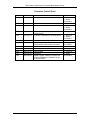
DATA PRODUCT SPECIFICATION
FOR COASTAL GLIDER DATA
PRODUCTS
Version 1-02
Document Control Number 1341-20001
2012-06-22
Consortium for Ocean Leadership
th
1201 New York Ave NW, 4 Floor, Washington DC 20005
www.OceanLeadership.org
in Cooperation with
University of California, San Diego
University of Washington
Woods Hole Oceanographic Institution
Oregon State University
Scripps Institution of Oceanography
Rutgers University
Data Product Specification for Coastal Glider Data Products
Document Control Sheet
Version
0-00
Date
2012-03-30
Description
Initial Release
0-01
0-02
2012-04-06
2012-04-09
Addition of DVL information
Review and editing
0-03
2012-04-10
0-04
2012-04-11
More edits, approaching rough draft for
outside review.
Final edits, draft ready for focused review
0-05
0-06
2012-04-12
2012-05-02
0-07
0-08
1-00
1-01
1-02
2012-05-07
2012-05-08
2012-05-16
2012-05-18
2012-06-22
Ver 1-02
Minor formatting changes.
Adjusted language for DBD and MBD files,
incorporated focused review comments
Comments and minor edits
Comments and edits incorporated
Initial Release
Formatting
Added magnetic variation correction and
changed ACBSCAT to ECHOINT as per
ECR 1300-00258
1341-20001
Author
C. Wingard,
C. Risien,
M. Vardaro
C. Risien
C. Wingard,
C. Risien,
M. Vardaro
C. Wingard
C. Wingard,
C. Risien,
M. Vardaro
S. Webster
C. Wingard,
M. Vardaro
S. Banahan
C. Wingard
E. Chapman
E. Griffin
M. Vardaro
i
Data Product Specification for Coastal Glider Data Products
Signature Page
This document has been reviewed and approved for release to Configuration Management.
OOI Senior Systems Engineer:
Date: 2012-05-16
This document has been reviewed and meets the needs of the OOI Cyberinfrastructure for the
purpose of coding and implementation.
OOI CI Signing Authority:
Date: 2012-05-16
Ver 1-02
1341-20001
ii
Data Product Specification for Coastal Glider Data Products
Table of Contents
1 Abstract ........................................................................................................................ 1 2 Introduction .................................................................................................................. 1 2.1 Author Contact Information ................................................................................... 1 2.2 Metadata Information ............................................................................................ 1 2.3 Instruments ........................................................................................................... 2 2.4 Literature and Reference Documents ................................................................... 2 2.5 Terminology .......................................................................................................... 3 3 Theory .......................................................................................................................... 4 3.1 Description ............................................................................................................ 4 3.2 Mathematical Theory ............................................................................................ 4 3.3 Known Theoretical Limitations .............................................................................. 6 3.4 Revision History .................................................................................................... 6 4 Implementation ............................................................................................................ 6 4.1 Overview ............................................................................................................... 6 4.2 Inputs .................................................................................................................... 6 4.3 Processing Flow ................................................................................................. 10 4.4 Outputs ............................................................................................................... 14 4.5 Computational and Numerical Considerations ................................................... 20 4.6 Code Verification and Test Data Set .................................................................. 20 Appendix A Example Code .......................................................................................... 1 Appendix B Output Accuracy ....................................................................................... 1 Appendix C Sensor Calibration Effects ........................................................................ 1 Ver 1-02
1341-20001
iii
Data Product Specification for Coastal Glider Data Products
1
Abstract
This document describes the processing steps required to extract the Level 0 and 1a OOI core
data products from binary data files logged on the Teledyne Webb Research (TWR) Slocum G2
Electric Glider, herein referred to as the Coastal Slocum Glider (CSG). These data products are
produced by the instruments and sensors integrated onto the CSG and are recorded and subsampled by the CSG in proprietary formats for near-real time and delayed (i.e., after CSG
recovery) data transmissions. This document is intended to be used by OOI programmers to
design and implement processes for the extraction of, and creation of, these data products, as
well as the archiving of relevant CSG engineering data for later use as metadata (e.g. time,
location and system health).
2
2.1
Introduction
Author Contact Information
Please contact Christopher Wingard ([email protected]) or the Data Product
Specification lead ([email protected]) for more information concerning the
computation and other items in this document.
2.2
Metadata Information
2.2.1 Data Product Name
The OOI Core Data Product Names, Descriptive Names and data product levels produced by the
instruments integrated onto the CSG are:
Data Product
Name
ECHOINT
VELPROF
CONDWAT
TEMPWAT
PRESWAT
DOCONCS
CDOMFLO
CHLAFLO
FLUBSCT
OPTPARW
Instrument
Class
ADCPA
ADCPA
CTDGV
CTDGV
CTDGV
DOSTA
FLORT
FLORT
FLORT
PARAD
Data Product Descriptive Name
Echo Intensity
Velocity Profiles
Conductivity
Temperature
Pressure (Depth)
Oxygen Concentration
Fluorometric CDOM Concentration
Fluorometric Chlorophyll-a Concentration
Optical Backscatter (red wavelengths)
Photosynthetically Active Radiation (PAR)
Data Product
Levels
Level 1a
Level 1a
Level 1a
Level 1a
Level 1a
Level 0 and 1a
Level 0 and 1a
Level 0 and 1a
Level 0 and 1a
Level 0 and 1a
2.2.2 Data Product Abstract (for Metadata)
See relevant Data Product Specifications for each data product. The Data Processing Flow
Diagram document numbers are included here as well for easy reference.
Data Product
Name
ECHOINT
VELPROF
CONDWAT
TEMPWAT
PRESWAT
DOCONCS
Ver 1-02
Data Product Spec.
Document Number
1341-00750
1341-00750
1341-00030
1341-00010
1341-00020
1341-00520
Instrument
Class
ADCPA
ADCPA
CTDGV
CTDGV
CTDGV
DOSTA
1341-20001
Data Processing Flow
Document Number
1342-00750
1342-00750
1342-00010
1342-00010
1342-00010
1342-00520
Page 1 of 20
Data Product Specification for Coastal Glider Data Products
CDOMFLO
CHLAFLO
FLUBSCT
OPTPARW
1341-00550
1341-00530
1341-00540
1341-00720
FLORT
FLORT
FLORT
PARAD
1342-00530
1342-00530
1342-00530
1342-00720
2.2.3 Computation Name
Not required for data products.
2.2.4 Computation Abstract (for Metadata)
This computation process converts the proprietary binary data files recorded by and on the CSG,
and extracts and computes the OOI Level 0 and 1a core data products using the primary (factory)
provided calibration coefficients and equations for each instrument, where applicable.
Additionally, CSG and instrument specific metadata is identified for use in subsequent L1-L2
processing and for CSG system health monitoring.
2.2.5 Instrument-Specific Metadata
The WET Labs ECO-Triplet (FLORT), the Aanderaa Optode 3835 or 4831 (DOSTA), the
Biospherical QSP-2150 PAR sensor (PARAD), and the Sea-Bird Electronics GPCTD (CTDGV) all
require primary (factory) calibration coefficients to convert the raw data signals to engineering
units. All of these calibration sheets are provided to CI as part of the instrument-specific
metadata.
The TRDI ExplorerDVL (ADCPA) does not require primary (factory) calibration coefficients to
convert the raw data signals to engineering units; all conversions and computations are
completed on the instrument itself with the results stored in binary data files. However,
information on the Doppler Velocity Log (DVL) operating parameters, pre-deployment
functionality checks, and internal compass calibrations are required metadata, and will be
provided to CI by the Implementing Organizations.
Pre and post-deployment functionality checks of all sensors and instruments, as well as
secondary calibrations (e.g. CSG and DVL compass calibrations and buoyancy checks predeployment), will be provided to CI for inclusion in the instrument-specific metadata.
2.2.6 Data Product Synonyms
See relevant Data Product Specifications for each data product.
2.2.7 Similar Data Products
See relevant Data Product Specifications for each data product.
2.3
Instruments
This document, in addition to the Coastal Glider Processing Flow document (DCN 1342-20001)
and the processing flow documents for the relevant instruments (see section 2.2.2), contains
information on the instruments from which the L0 and L1a core data products are obtained.
Please see the Instrument Application in the SAF for specifics of instrument locations and
platforms.
2.4
Literature and Reference Documents
Aanderaa (2007). TD 218 Operating Manual Oxygen Optode 3830, 3835, 3930, 3975, 4130,
4175. Aanderaa Data Instruments.
(see REFERENCE >> Instrument and Vehicle Documents >> Coastal Glider >>
3830_optode_manual.pdf)
Ver 1-02
1341-20001
Page 2 of 20
Data Product Specification for Coastal Glider Data Products
Biospherical (2011). QSP-2150 and QCP-2150 Submersible PAR Sensors with ASCII Output
User's Manual. Biospherical Instruments, Inc.
(see REFERENCE >> Instrument and Vehicle Documents >> Coastal Glider >>
QSP_2150_Manual.pdf)
Sea-Bird (2010). Glider Payload CTD (GPCTD) and Optional DO Sensor, User’s Manual Version
#001. Sea-Bird Electronics, Inc.
(see REFERENCE >> Instrument and Vehicle Documents >> Coastal Glider >>
GliderPayloadCTD_001.pdf)
Teledyne RDI (2009). RDI Tools User's Guide, P/N 957-6157-00. Teledyne RD Instruments, Inc.
(see REFERENCE >> Instrument and Vehicle Documents >> Coastal Glider
>>RDI_Tools_User_Guide.pdf)
Teledyne RDI (2010). ExplorerDVL Operation Manual, P/N 95B-6027-00. Teledyne RD
Instruments, Inc.
(see REFERENCE >> Instrument and Vehicle Documents >> Coastal Glider >>
Explorer_Operation_Manual.pdf)
TWR (2010). Dock Server User Guide, Revision 7.4. Teledyne Webb Research.
(see REFERENCE >> Instrument and Vehicle Documents >> Coastal Glider >>
gmcUserGuide.pdf)
TWR (2012). Slocum G2 Glider Maintenance Manual, P/N 4344, Rev. B. Teledyne Webb
Research.
(see REFERENCE >> Instrument and Vehicle Documents >> Coastal Glider >>
4344_Rev.B-Slocum_Glider_Maintenance_Manual.pdf)
TWR (2012). Slocum G2 Glider Operations Manual, P/N 4343, Rev. B. Teledyne Webb
Research.
(see REFERENCE >> Instrument and Vehicle Documents >> Coastal Glider >>
4343_Rev.B-Slocum_Glider_Operators_Manual.pdf)
WET Labs (2010). ECO Three-Measurement Sensor Triplet Puck, User’s Guide Revision G.
WET Labs, Inc.
(see REFERENCE >> Instrument and Vehicle Documents >> Coastal Glider >>
tripletpuckg.pdf) 2.5
Terminology
2.5.1 Definitions
The following terms are defined here for use throughout this document. Definitions of general
OOI terminology are contained in the Level 2 Reference Module in the OOI requirements
database (DOORS).
Ensemble: Collection of 3 or more DVL velocity pings averaged together to produce a velocity
profile with associated depth, temperature, acoustic backscatter, and signal quality information.
Velocity Profile: One averaged DVL ensemble that provides relative u and v velocities in m/s.
2.5.2 Acronyms, Abbreviations and Notations
General OOI acronyms, abbreviations and notations are contained in the Level 2 Reference
Module in the OOI requirements database (DOORS). The following acronyms and abbreviations
are defined here for use throughout this document.
ADCP
CF
CSG
DBD
DO
DVL
TRDI
Ver 1-02
Acoustic Doppler Current Profiler
Compact Flash
Coastal Slocum Glider
Dinkum Binary Data
Dissolved Oxygen
Doppler Velocity Log
Teledyne RD Instruments
1341-20001
Page 3 of 20
Data Product Specification for Coastal Glider Data Products
TWR
Teledyne Webb Research
2.5.3 Variables and Symbols
The following variables and symbols are defined here for use throughout this document.
offset
sfactor
Baseline offset subtracted from the the L0 data products
Scale factor to multiply offset-corrected L0 data products.
All offsets and scaling factors are on the instrument specific calibration sheets that are part of the
instrument-specific metadata.
3
3.1
Theory
Description
The CSG serves as the platform controller for the suite of attached and integrated instruments
and sensors on the CSG; controlling not only how and where the CSG travels while deployed, but
also when instruments and sensors on the CSG are powered, how and what data variables are
recorded, and at what rate the data streams from the instruments and sensors are sampled and
telemetered to shore. With the exception of the DVL, all of the instruments and sensors
integrated onto the CSG report their data directly to the CSG, where it is converted into a
transmittable and storable form.
The instrument and sensor data streams are sampled by the CSG at rates equal to or less than
the individual instrument data rates, with the resulting recorded data stored in CSG data variables
and written to data files on the CSG. All of the data files are stored on CF cards within the CSG
in proprietary binary data formats. Most of the data is stored in the Dinkum Binary Data (DBD)
format used by TWR. The DVL data, the exception noted above, is stored by the CSG on the CF
card in the proprietary, native “PD0” file format for the DVL without being read or sampled by the
CSG. Data is never streamed from a CSG, instead the stored data files are either transferred to
shore at semi-regular intervals, or downloaded from the CSG after a deployment.
To obtain the L0 and L1a data products from the CSG, it is first necessary to convert the DBD
and PD0 files to a format accessible by CI and then to map the appropriate CSG and DVL
variables to the core data products.
3.2
Mathematical Theory
The CSG is received by OOI already pre-calibrated by TWR, with the integrated instruments and
sensors serviced and calibrated as appropriate by TWR and the respective instrument
manufacturers before the initial deployment. Post-initial deployment recalibrations will be
performed at TWR, with the individual instruments returned to the respective manufacturer for
service and recalibration. The different instruments on the CSG report their data to the CSG at
either Level 0, Level 1a, or both. Thus, processing the data begins with extracting and mapping
the named variables to the appropriate OOI core data product, and applying calibration,
conversion and scaling factors where appropriate. These are described below with the units of
measurement and variable names provided in Section 4.3.
For all instruments that report both L0 and L1a data products, the L1a data will be telemetered to
shore in the near real-time data files (the decimated .sbd and .tbd files described below in Table
4-1). The L0 product will only be included in the data files downloaded from a glider after
recovery.
3.2.1 Sea-Bird GPCTD (CTDGV)
The conductivity (CONDWAT), temperature (TEMPWAT) and pressure (PRESWAT) data
recorded by the Sea-Bird GPCTD are reported to the CSG already converted to science units
Ver 1-02
1341-20001
Page 4 of 20
Data Product Specification for Coastal Glider Data Products
(S/m, °C, and bar, respectively) by calibration coefficients entered directly onto the GPCTD at the
factory. No further processing beyond mapping the named glider variables for the GPCTD to the
L1a data products is required.
The processing flow for Level 1 CTDGV data products through to Level 2 Density and Salinity
data products is further described in CTD Data Processing Flow (DCN 1342-00001), Data
Product Specification for Conductivity Compressibility Compensation (DCN 1341-10030), Data
Product Specification for Density (DCN 1341-00050), and Data Product Specification for Salinity
(DCN 1341-00040).
3.2.2 WET Labs ECO Triplet (FLORT)
The CDOM (CDOMFLO), chlorophyll (CHLAFLO) fluorescence, and optical backscatter
(FLUBSCT) data are reported by the ECO Triplet to the CSG as both L0 and L1a data products.
The conversion from L0 to L1a for all three data products is defined below:
L1a_Data_Product = (L0_Data_Product - offset) * sfactor
Where the L0_Data_Product is measured in counts, and the offset and sfactor are from
the factory supplied calibration worksheets for the ECO Triplet. These calibration sheets are
provided to CI as part of the instrument-specific metadata.
The processing flow for L1 CDOMFLO and CHLAFLO data products is further described in
FLORT Data Processing Flow (DCN 1342-00530), Data Product Specification for CDOMFLO
(DCN 1341-00550) and Data Product Specification for CHLAFLO (DCN 1341-00530).
3.2.3 Biospherical QSP-2150 PAR (PARAD)
The PAR (OPTPARW) data is reported by the QSP-2150 to the CSG as both L0 and L1a data
products. The conversion from L0 to L1a is defined below:
L1a_Data_Product = (L0_Data_Product - offset) / sfactor
Where the L0_Data_Product is measured in volts, and the offset and sfactor are from
the factory supplied calibration worksheet for the QSP-2150. The calibration sheet is provided to
CI as part of the instrument-specific metadata.
The processing flow for Level 1 PARAD data products is further described in PARAD Data
Processing Flow (DCN 1342-00720).
3.2.4 Aanderaa Optode 3835/4831 (DOSTA)
The first article glider will contain an Aanderaa 3835 optode, while all subsequently procured
gliders will incorporate the Aanderaa 4831 optode. Both optodes operate the same firmware, and
require the same data processing. The DO (DOCONCS) data is reported by the Aanderaa 3835
or 4831 to the CSG as both an L0 and L1a data product. The L0 product is processed using the
same algorithm as described in the DOCONCS Data Product Specification (DCN 1341-00520) to
convert from optode phase to oxygen concentration in µmol/L or µmol/kg. This algorithm uses L1
pressure (PRESWAT), L2 salinity (PRACSAL), and L2 density (DENSITY) inputs from the SeaBird GPCTD to produce the L2 DOCONCS data product.
The processing flow for L1 and L2 DOCONCS data product levels is further described in the
DOSTA Data Processing Flow (DCN 1342-00520).
3.2.5 TRDI ExplorerDVL (ADCPA)
The core data products associated with the DVL (ADCPA) are the velocity profile (VELPROF)
data, which include east-west and north-south velocities, and the echo intensity (ECHOINT) data.
Ver 1-02
1341-20001
Page 5 of 20
Data Product Specification for Coastal Glider Data Products
These data are reported by the DVL as L1a data products. The ADCPA VELPROF data are then
corrected for magnetic variation as outlined in the VELPROF DPS (1341-00750, Step 8) and go
through the QC processing flow outlined in the VELPROF processing flow diagram (1342-00750).
3.3
Known Theoretical Limitations
No known theoretical limitations.
3.4
Revision History
No revisions to date.
4
Implementation
4.1
Overview
The conversion of the CSG binary data files (DBD formatted) to a format accessible by CI is
accomplished by the use of the TWR provided proprietary applications (available for computers
with either a Windows or Linux OS installed). The same utilities are used regardless of the
source or type of DBD file (e.g. Flight versus Science). PD0 files can be read and the data
rd
extracted using TRDI applications such as WinADCP as well as 3 party applications such as
®
MATLAB from Mathworks, Inc.
The computation described herein only extracts the data from the binary files and maps the
extracted variables to core Level 0 and 1a data products where appropriate. Additionally, key
metadata elements (time, location and system health) are identified.
4.2
Inputs
All inputs for this DPS are the binary files uploaded from the CSG and encoded with the
manufacturer’s proprietary format (DBD files for the CSG and PD0 for the DVL), requiring the use
of the respective instrument manufacturer’s proprietary software tools to extract the data. The
data files are uploaded to shore and then to CI in either near real-time (via the Iridium satellite
network), or in the lab after the CSG is recovered. There are three classes of available CSG data
files with different file extensions (aka types, see Table 4-1) depending on where the data is
recorded and their contents. These are:
•
•
•
CSG Flight (Engineering) Data Files: Engineering data, recorded in proprietary DBD
formatted files on the CF card in the Engineering Bay of the CSG.
CSG Science Data Files: Instrument data recorded in proprietary DBD formatted files on
the CF card in the Science Bay of the CSG.
CSG TRDI ExplorerDVL Data Files: Data files from the DVL recorded on the CF card in
the Science Bay of the CSG.
Ver 1-02
1341-20001
Page 6 of 20
Data Product Specification for Coastal Glider Data Products
Table 4-1. File classes and types recorded by the CSG.
Class
Flight
File Type
.dbd
Flight
.mbd
Flight
.sbd
Science
.ebd
Science
.nbd
Science
.tbd
DVL
.pd0
Description
Dinkum binary data -- all sensors and variables in the masterdata
configuration file are recorded in these data file types at the full
sampling rate specified in the glider configuration files prior to
mission execution. These are large files and would not be
normally transmitted over the satellite network.
Medium binary data -- a user specified list of sensors or variables
to record (specified in mbdlist.dat); constitutes a decimated
version in the number of variables of the .dbd file. Not normally
transmitted during a mission due to size; only sent if a need exists
for a more detailed near real-time data sets.
Short binary data -- a user specified list of sensors or variables to
record (specified in sbdlist.dat); constitutes a small, decimated
version (in both the sample rate and and the number of variables)
of the .dbd file. Normally transmitted during a mission over the
Iridium satellite network. Limited to key sensors and minimal
sample rates to minimize satellite airtime use while still permitting
piloting functions and basic environmental monitoring.
Equivalent to .dbd files for all science instruments integrated onto
the CSG.
Equivalent to .mbd files for all science instruments. Specified in
nbdlist.dat and references the .ebd files.
Equivalent to .sbd files for all science instruments. Specified in
tbdlist.dat and references the .ebd files.
Binary encoded data files from the DVL in the proprietary format
used by TRDI.
The .dbd files described above in Table 4-1 currently consist of 1879 named variables. The
sampled variables represent all of the potential instruments and variables that a CSG could be
configured with, and are listed in the "masterdata" configuration file used by all CSG. Many of
those variables do not pertain to OOI as they reference sensors and instruments that are unlikely
to be installed on the CSG, are recorded in the .ebd, are used to configure simulations, or are
factory calibration values that can be obtained from the original calibration documentation. These
files have the potential to be quite large. A list of all of the variables available in the DBD files
(from both the Flight and Science data files) is available for review in a spreadsheet
(CSG_Flight_Science_Variables_2012-04-09_ver_1-00.xlsx) on Alfresco at REFERENCE >>
DPS Artifacts >> CSTGLDR_Data_Test.zip.
The CSG operating system automatically manages the storage and transmission of the DBD files.
Recorded files are stored in the LOGS directory on both the Science and Flight CF cards. Once
the file is successfully transmitted to shore, it is moved to the SENTLOGS directory. In the case of
the Flight data files (the .dbd, .mbd and .sbd files), the potential exists for automatic deletion of
the .dbd files if the CF card capacity (2 GB) is reached. The sequence of automatic file deletion
is to clear the SENTLOGS directory first. If more space is needed, the .dbd files will be deleted on
a "first in, first out" basis.
In order to limit the number of variables that must be tracked and to avoid the potential loss of
data as noted above, the .mbd files shall be used to record only those variables that directly map
to instruments and sensors installed on the CSG. The spreadsheet described above will be used
by CSG pilots to determine the essential variables needed in the .mbd/.nbd and .sbd/.tbd data
files; variables that are used for CSG piloting and provide basic environmental monitoring. All
recorded DBD files, regardless of their content, will be transferred to CI for archiving.
Ver 1-02
1341-20001
Page 7 of 20
Data Product Specification for Coastal Glider Data Products
CSG deployments are organized into missions, which themselves contain individual segments.
The CSG data files are named using the following two conventions according to the mission and
segment numbers:
• On the CSG, data files are named according to an 8.3 convention in which the first 4
numbers correspond to the sequential mission number and the last 4 numbers
correspond to the sequential segment number of the current mission.
• The same data files, once transferred to shore, are automatically renamed by the Dock
Server application according to the following convention:
gliderName_yyyy_ddd_mmm_sss.*bd
where gliderName is the name of the glider, yyyy is the current year, ddd is the (0based) day of the year, mmm is the (0-based) mission number for the current day of the
year, sss is the (0-based) segment number of the current mission, and .*bd is the file
type as described above.
The latter file naming convention will apply to the data files sent to CI. The 8.3 files are
automatically renamed to the second format after uploading to shore-side servers with the TWR
Dock Server and Data Server applications installed. If the file is incomplete or contains no data, it
will not be renamed. Thus, files named using the 8.3 format that are delivered to CI are to be
considered incomplete and should be ignored.
The DVL generates multiple PD0 files, with each PD0 file containing multiple ensembles. PD0
files are binary files encoded using TRDI’s proprietary format. Due to DVL power usage, the DVL
data will be recorded during a CSG downcast or descent only, skipping downcasts so every other
rd
th
or 3 or 4 descent is recorded. The file naming convention used for PD0 files is
YMDDHHMM.PD0, where:
Y = year (TRDI uses a-z to indicate year with a=2001, b=2002,…, z=2026)
M = month (TRDI uses a-l to indicate month with a=January, b=February,…, l=December)
DD = day of the month
HH = hour
MM = minute
Input Data Formats:
The formatting of the PD0 data files is fully described in Section 12 of the TRDI ExplorerDVL
operations manual. These files can be read, and the data extracted from them, as noted above,
rd
®
using TRDI applications such as WinADCP, as well as 3 party applications such as MATLAB
from Mathworks, Inc. How to read and extract the data from the PD0 files using MATLAB is
described in detail below.
TWR does not provide information on the exact formatting of the DBD files. A general description
of the files can be found in the TWR Operations manual. All DBD files consist of an ASCII header
followed by the binary formatted data. The ASCII header consists of two parts: the first 14 lines
followed by the remainder which is dependent on the number of variables recorded and is only
included in the first segment file for a mission. The first part (Table 4-2) includes information on
the file (when it was recorded, what the file type is, etc), and the second part (Table 4-3) lists the
recorded variables.
Ver 1-02
1341-20001
Page 8 of 20
Data Product Specification for Coastal Glider Data Products
Table 4-2. Part 1 of the DBD ASCII header recorded at the beginning of all DBD files.
Tag Comments (not part of file) dbd_label: DBD(dinkum_binary_data)file File formatting -­‐-­‐ binary encoding_ver: 5 num_ascii_tags: 14 # of recorded variables all_sensors: F All sensors recorded? True/False the8x3_filename: 1380000 File name used on CSG full_filename: unit_247-­‐2012-­‐008-­‐7-­‐0 filename_extension: tbd mission_name: INI50W.MI CSG mission file used fileopen_time: Mon_Jan__9_19:06:10_2012 Date file opened for recording total_num_sensors: 91 # of variables available to record sensors_per_cycle: 14 # of actually recorded variables state_bytes_per_cycle: 4 sensor_list_crc: 1DE45D61 sensor_list_factored: 0 List of sensors is factored (0 if first segment of mission) Ver 1-02
Value 1341-20001
Page 9 of 20
Data Product Specification for Coastal Glider Data Products
Table 4-3. Part 2 of the ASCII header, only recorded in the first segment file for a mission. The
second part of the DBD ASCII header details the list of available sensors (variables), whether
they are actually recorded, the order of the variables in the file (0-based, negative numbers are
not recorded), the number of bytes per variable, the variable name as recorded by the CSG and
the units of the recorded variable.
Tag Recorded Variable# Index# #Bytes Variable Name s: F 0 -­‐1 1 sci_bsipar_is_installed s: T 1 0 4 sci_bsipar_par s: T 2 1 4 sci_bsipar_sensor_volts s: F 3 -­‐1 4 sci_bsipar_supply_volts s: T 4 2 4 sci_bsipar_temp <-­‐-­‐ Full list of variables not included for the sake of brevity -­‐-­‐> s: T 86 11 4 sci_water_cond s: T 87 12 4 sci_water_pressure s: T 88 13 4 sci_water_temp s: F 89 -­‐1 4 sci_x_disk_files_removed s: F 90 -­‐1 4 sci_x_sent_data_files 4.3
Units bool ue/m^2sec volts volts Degc s/m bar degc nodim nodim Processing Flow
The specific steps necessary to create all calibrated and quality controlled data products for each
OOI core instrument are described in the instrument-specific Processing Flow documents noted
above in Section 3.2. These processing flow documents contain flow diagrams detailing all of the
specific procedures (data product and QA/QC) necessary to compute all data products from the
instruments and the order in which these procedures are applied.
The processing flow for converting the DBD files and registering the L0 and L1a data products
and metadata elements is:
Step 1: Convert the DBD files to ASCII and import them into MATLAB.
All DBD files are converted and imported into MATLAB using the same TWR provided utilities,
which can be called from either within MATLAB (see Appendix A.1) or from the command line in a
terminal window.
Step 2: Map Science variables to core data products, scaling and converting where applicable.
For all .ebd, .nbd and .tbd files, the CSG Science data variables produced by executing the
example code in Appendix A.1 are listed in Table 4-4 with their mapping to the core L0 and L1a
data products.
Ver 1-02
1341-20001
Page 10 of 20
Data Product Specification for Coastal Glider Data Products
Table 4-4. Level 0 and 1a core data products in the CSG Science data files.
Data
Product
CONDWAT
TEMPWAT
PRESWAT
Data
Source
CTDGV
CTDGV
CTDGV
Data
Level
1a
1a
1a
Units
Variable Name
S/m
°C
bar
sci_water_cond
sci_water_temp
sci_water_pressure
DOCONCS
DOSTA
0
1a
1a
n/a
µM
%
sci_oxy3835_wphase_dphase
sci_oxy3835_wphase_oxygen
sci_oxy3835_wphase_saturation
CDOMFLO
FLORT
CHLAFLO
FLORT
FLUBSCT
FLORT
0
1a
0
1a
0
1a
counts
ppb
counts
µg/l
counts
-1
-1
m sr
sci_flbbcd_cdom_sig
sci_flbbcd_cdom_units
sci_flbbcd_chlor_sig
sci_flbbcd_chlor_units
sci_flbbcd_bb_sig
sci_flbbcd_bb_units
OPTPARW
PARAD
0
1a
volts
-2 -1
µE m s
sci_bsipar_sensor_volts
sci_bsipar_par
Comments
Scale to
decibar [db] by
multiplying by
10.
L0 data can be
used to derive
all L1 and L2
data products
after glider
recovery.
L1a is the total
volume
scattering
coefficient,
-1
-1
β(θ,λ) [m sr ],
where θ = 117°
and λ = 700
nm.
Step 3: Map Flight variables to key metadata elements.
For the .dbd, .mbd and .sbd files, all of the recorded variables constitutes the engineering (Flight)
data for a CSG, and as such must be preserved as metadata. Certain variables are critical
(providing information on the time and location of data collection) and need to be mapped to
specific metadata elements for further Level 1 and 2 processing of the data products produced by
the CSG, in addition to being available for CSG piloting functions (system health
monitoring)(Table 4-5). All of these variables are recorded in the .dbd and .mbd files, while a
subset are available in the .sbd files.
Table 4-5. Flight (engineering) data used for processing Level 1 data products (time and location
variables) and for system health monitoring.
Variable Name
m_present_time
m_present_secs_into_mission
m_gps_utc_year
m_gps_utc_month
m_gps_utc_day
m_gps_utc_hour
Ver 1-02
Description
Seconds since January 1, 1970
Elapsed mission time
GPS derived current year (UTC).
GPS measurements only occur
when CSG is at the surface.
GPS month (01-12) of the year
(UTC)
GPS day (01-31) of the month
(UTC)
GPS hour (00-23) of the day
(UTC)
1341-20001
Units
seconds
seconds
year
month
day
hour
Page 11 of 20
Data Product Specification for Coastal Glider Data Products
m_gps_utc_minute
m_gps_utc_second
m_gps_lat
m_gps_lon
m_gps_heading
m_gps_mag_var
m_gps_speed
c_heading
m_heading
c_pitch
m_pitch
m_roll
m_lat
m_lon
m_depth
m_altitude
m_altitude_raw
m_water_depth
m_system_clock_lags_gps
m_avg_system_clock_lags_gps(sec)
m_battery
m_coulomb_amphr
m_coulomb_amphr_total
m_lithium_battery_relative_charge
c_ballast_pumped
m_ballast_pumped
c_de_oil_vol
m_de_oil_vol
c_air_pump
m_air_pump
m_vacuum
c_wpt_lat
c_wpt_lon
x_last_wpt_lat
x_last_wpt_lat
m_tot_num_inflections
Ver 1-02
GPS minute (00-59) of the hour
(UTC)
GPS seconds (00-59) of the
minute (UTC)
GPS determined latitude of form
±DDMM.MMMM, where values > 0
are recorded in the northern
hemisphere.
GPS determined longitude of form
±DDDMM.MMMM, where values >
0 are recorded east of the Prime
Meridian.
GPS heading
GPS magnetic variation used to
correct compass headings to true
north
GPS estimated speed over ground
Commanded CSG heading
Measured CSG heading
Commanded CSG pitch
Measured CSG pitch
Measured CSG roll
Estimated latitude while CSG is
underwater, derived from dead
reckoning.
Estimated longitude while CSG is
underwater, derived from dead
reckoning.
CSG
Filtered height above the bottom
Raw, unfiltered height above the
bottom
Total water column depth
Instant offset between CSG real
time clock and GPS
Averaged offset between CSG and
real time clock, if exceeds 12
seconds the clock is reset
Voltage level of battery pack
Instant current usage of battery
pack
Cumulative current usage of
battery pack
Remaining battery charge
minute
Internal vacuum pressure
Current waypoint, latitude
Current waypoint, longitude
Last waypoint, latitude
Last waypoint, longitude
Number of inflections for buoyancy
psi
1341-20001
seconds
degrees
and
minutes
degrees
and
minutes
degrees
degrees
knots
degrees
degrees
degrees
degrees
degrees
degrees
and
minutes
degrees
and
minutes
meters
meters
meters
meters
seconds
seconds
volts
amphours
amphours
%
Page 12 of 20
Data Product Specification for Coastal Glider Data Products
m_final_water_vx
m_final_water_vy
m_water_vx
m_water_vy
m_leak_detect_voltage
m_leak_detect_voltage_forward
pump. Max is 20,000 before
replacement.
Water column averaged velocity
Leak detect voltage in aft section
of CSG. Values below 2.0 volts
indicate a leak condition. Nominal
is 2.4 volts.
Leak detect voltage in forward
section of CSG. Values below 2.0
volts indicate a leak condition.
Nominal is 2.4 volts.
m/s
m/s
m/s
m/s
volts
volts
Step 4: Convert PD0 files.
Appendix A.2 and A.3 contain example MATLAB functions that read and extract data and
metadata from PD0 files.
Step 5: Map PD0 data file variables to core OOI data products.
Step 6: Use equation 5 specified in Step 8 of the VELPROF DPS (1341-00750) to correct for
magnetic variation in the u and v velocity components.
Step 7: See CSGLIDR Processing Flow document (DCN 1342-20001) and VELPROF Processing
Flow Document (DCN 1342-00750) for additional post-processing steps.
The PD0 data variables produced by executing the example code in Appendix A.2 and A.3 are
listed in Table 4-6 with their mapping to the core L0 and L1a data products.
Ver 1-02
1341-20001
Page 13 of 20
Data Product Specification for Coastal Glider Data Products
Table 4-6. Level 1a core data products in the extracted from the DVL data files logged by the
CSG.
Data
Product
VELPROF
Data
Source
ADCPA
Data
Level
1a
Units
m/s
Variable Name
u_velocities
VELPROF
ADCPA
1a
m/s
v_velocities
VELPROF
ADCPA
1a
m/s
w_velocities
ECHOINT
ADCPA
1a
dB
echo_1
ECHOINT
ADCPA
1a
dB
echo_2
ECHOINT
ADCPA
1a
dB
echo_3
ECHOINT
ADCPA
1a
dB
echo_4
4.4
Comments
Relative
East/West
velocity profiles
Relative
north/south
velocity profiles
Relative vertical
velocity profiles
Echo intensity
profile for beam
1
Echo intensity
profile for beam
2
Echo intensity
profile for beam
3
Echo intensity
profile for beam
4
Outputs
4.4.1 DBD (CSTGLDR) Output
The outputs of the extraction and mapping computation for the DBD files are the OOI L0 and L1a
core data products as defined above and are available for further L1 and L2 processing as
applicable. These data products are extracted from the Science data (.ebd, .nbd and .tbd) files.
All other variables in the Science data files not mapped as described in Table 4-4 above are to be
retained in the archived DBD data files for future possible use.
The metadata that must be included with the output is defined in Table 4-5 above and is
extracted from the Flight data files (.dbd, .mbd and .sbd). As with the Science data files, all of the
Flight DBD files are to be archived for future possible use.
Example output from the extraction of the DBD file is provided with the test data set (unit_2472012-008-8-0.tbd) for review. The example code in Appendix A.1 results in the production of an
m-file (MATLAB script file) with the same name as the glider data file (the '.' in the file name are
replaced with '_' and a '_gld' is appended to the end of the file name) that creates a structured
array listing the data variables in the file and their order (parses the ASCII header of the file).
Additionally, the data portion of the file is placed in an ASCII, tab-delimited .dat file with the
same name as the m-file. Running the created m-file (type run(fileName); at the MATLAB
prompt after running the example in Appendix A.1), loads the data and the structured array with
the header information into the workspace. Execution of the code in Appendix A.1 should
produce results that are identical to those described below in Table 4-7.
Ver 1-02
1341-20001
Page 14 of 20
Data Product Specification for Coastal Glider Data Products
Table 4-7. Output variables available in the MATLAB workspace from the conversion and
extraction of the binary data in the provided example DBD file.
Workspace Variable
Data
run_name
sensor_lookup
Array Size
76x14
Array Type
1x1
4.4.2 PD0 (ADCPA) Output
The code examples in Appendix A.2 and A.3 produce a MATLAB structured array (dvl), the
contents of which are described in Table 4-8.
Table 4-8. MATLAB workspace variables created after executing the example code in Appendix
A.3. ADCPA Level 1a core data products (VELPROF and ECHOINT), as well as key metadata
products that will be needed for further L1 processing, are highlighted in bold text.
Workspace
Array
Array
Description
Units
Variable
Size
Type
n_cells
1x3728
double
Contains the number of depth cells over
count
which the ExplorerDVL collects data
pings_per_ens
1x3728
double
Contains the number of pings averaged
count
together during a data ensemble
cell_size
1x3728
double
Contains the length of one depth cell
meters
blank
1x3728
double
time_btwn_pings
1x3728
double
coord_system
'earth'
string
bin1_dist
1x3728
double
xmit_pulse
1x3728
double
xmit_lag
1x3728
double
ranges
3728x15
double
ensb
rtc
1x3728
7x3728
double
double
transducer_depth
1x3728
double
pitch
1x3728
double
Contains the blanking distance used by
the ExplorerDVL to allow the transmit
circuits time to recover before the
receive cycle begins
Contains the minimum time between
pings
Contains the coordinate transformation
processing parameters
Contains the distance to the middle of
the first depth cell (bin)
Contains the length of the transmit
pulse
Contains the distance between pulse
repetitions
Contains the distance to the middle of
each bin
Contains ensemble number
Contains year, month, day, hour,
minute, second, hundredths of a
second information used to calculate
dvl.time, which is a Matlab serial date
number. The ExplorerDVL does
account for leap years.
Contains the depth of the transducer
below the water surface
Contains the ExplorerDVL pitch angle
roll
1x3728
double
Contains the ExplorerDVL roll angle
degrees
heading
1x3728
double
degrees
temperature
1x3728
double
Contains the ExplorerDVL heading
angle
Contains the temperature of the water
at the transducer head
Ver 1-02
1341-20001
meters
seconds
N/A
meters
meters
meters
meters
count
years, months,
days, hours,
minutes,
seconds,
hundredths of
a second
meters
degrees
degree
Celsius
Page 15 of 20
Data Product Specification for Coastal Glider Data Products
salinity
1x3728
double
heading_std
1x3728
double
pitch_std
1x3728
double
roll_std
1x3728
double
speed_of_sound
1x3728
double
u_velocities
15x3728
double
v_velocities
15x3728
double
w_velocities
15x3728
double
error_velocities
15x3728
double
corr1
15x3728
double
corr2
15x3728
double
corr3
15x3728
double
corr4
15x3728
double
echo1
15x3728
double
echo2
15x3728
double
echo3
15x3728
double
echo4
15x3728
double
pg1
15x3728
double
pg2
15x3728
double
pg3
15x3728
double
pg4
15x3728
double
btppe1
1x3728
double
btrange1
1x3728
double
btrange2
1x3728
double
btrange3
1x3728
double
Ver 1-02
Contains the salinity value of the water
at the transducer head
Contains the standard deviation of the
ExplorerDVL heading angle
Contains the standard deviation of the
ExplorerDVL pitch angle
Contains the standard deviation of the
ExplorerDVL roll angle
Contains speed of sound information
Contains relative east-west water
velocities
Contains relative north-south water
velocities
Contains relative vertical water
velocities
Contains water error velocities
Contains the correlation magnitude
data for beam #1
Contains the correlation magnitude
data for beam #2
Contains the correlation magnitude
data for beam #3
Contains the correlation magnitude
data for beam #4
Contains the echo intensity data
for beam #1
Contains the echo intensity data
for beam #2
Contains the echo intensity data
for beam #3
Contains the echo intensity data
for beam #4
Percentage of good 3-beam solutions
Percentage of transformations rejected
Percentage of more than one beam bad
in bin
Percentage of good 4-beam solutions
Contains the number of bottom-track
pings to average together in each
ensemble
Contains the two lower bytes of the
vertical range from the ExplorerDVL to
the sea bottom as determined by beam
#1
Contains the two lower bytes of the
vertical range from the ExplorerDVL to
the sea bottom as determined by beam
#2
Contains the two lower bytes of the
vertical range from the ExplorerDVL to
the sea bottom as determined by beam
#3
1341-20001
N/A
degrees
degrees
degrees
m/s
m/s
m/s
m/s
m/s
N/A
N/A
N/A
N/A
dB
dB
dB
dB
%
%
%
%
count
meters
meters
meters
Page 16 of 20
Data Product Specification for Coastal Glider Data Products
btrange4
1x3728
double
meters/second
double
Contains the two lower bytes of the
vertical range from the ExplorerDVL to
the sea bottom as determined by beam
#4
Contains bottom track east-west
velocities
Contains bottom track north-south
velocities
Contains bottom track vertical velocities
Btu
1x3728
double
Btv
1x3728
double
Btw
1x3728
btvelerr
1x3728
double
Contains bottom track error velocities
meters/second
btcorr1
1x3728
double
btcorr2
1x3728
double
btcorr3
1x3728
double
btcorr4
1x3728
double
btampl1
1x3728
double
btampl2
1x3728
double
btampl3
1x3728
double
btampl4
1x3728
double
btpg1
1x3728
double
btpg2
1x3728
double
btpg3
1x3728
double
btpg4
1x3728
double
btrange_msb1
1x3728
double
btrange_msb2
1x3728
double
Contains the correlation magnitude in
relation to the sea bottom as
determined by beam #1
Contains the correlation magnitude in
relation to the sea bottom as
determined by beam #2
Contains the correlation magnitude in
relation to the sea bottom as
determined by beam #3
Contains the correlation magnitude in
relation to the sea bottom as
determined by beam #4
Contains the beam #1 evaluation
amplitude of the matching filter used in
determining the strength of the bottom
echo
Contains the beam #2 evaluation
amplitude of the matching filter used in
determining the strength of the bottom
echo
Contains the beam #3 evaluation
amplitude of the matching filter used in
determining the strength of the bottom
echo
Contains the beam #4 evaluation
amplitude of the matching filter used in
determining the strength of the bottom
echo
Contains percent-good data for the
water mass for beam # 1
Contains percent-good data for the
water mass for beam # 2
Contains percent-good data for the
water mass for beam # 3
Contains percent-good data for the
water mass for beam # 4
Contains the most significant byte of
the vertical range from the ExplorerDVL
to the sea bottom as determined by
beam #1
Contains the most significant byte of
the vertical range from the ExplorerDVL
to the sea bottom as determined by
beam #2
Ver 1-02
1341-20001
meters
meters/second
meters/second
N/A
N/A
N/A
N/A
counts
counts
counts
counts
%
%
%
%
meters
meters
Page 17 of 20
Data Product Specification for Coastal Glider Data Products
btrange_msb3
1x3728
double
btrange_msb4
1x3728
double
time
1x3728
double
bin_depth
15x3728
double
Contains the most significant byte of
the vertical range from the ExplorerDVL
to the sea bottom as determined by
beam #3
Contains the most significant byte of
the vertical range from the ExplorerDVL
to the sea bottom as determined by
beam #4
Contains MATLAB serial date
numbers for each ensemble
Contains the water depth for each
bin for each ensemble
meters
meters
Days since
Jan-1-0000
00:00:00
meters
In this example, the glider began its dive on February 14, 2012 at 13:48:41 and ended its dive at
February 14, 2012 at 15:25:46. For this particular dive the glider decended to approximately
982.3 meters. This glider depth information is contained in the “dvl.transducer_depth” array.
During the descent, 3728 ensemble averages were recorded. Each ensemble average contains,
amongst other things, one velocity profile (relative u and v velocities given in mm/s) as well as
four acoustic backscatter profiles, one for each beam, given in decibels (dB). Each profile
contains 15 bins or depth cells. The bin size is 2 meters. The center of the first bin for ensemble
#1 is located 2.97 meters below the transducer (see Figure 4-1).
Figure 4-1. Schematic showing DVL bins and bin depths relative to the transducer for ensemble
#1 of file lb141348.pd0.
To confirm that the velocity data are being read correctly, Table 4-9 shows the center-bin depths
and relative "u" and "v" velocities for all 15 bins for ensemble 300, which was recorded on
February 14, 2012 at 13:56:46 when the transducer was at a depth of 39.5 meters. Note that
these velocities are in Earth coordinates. Table 4-10 shows the center-bin depths and acoustic
backscatter profiles (one for each beam) for all 15 bins for ensemble 300.
Ver 1-02
1341-20001
Page 18 of 20
Data Product Specification for Coastal Glider Data Products
Table 4-9. Center-bin depths and relative u and v velocities for all 15 bins for ensemble 300
which was recorded on February 14, 2012 at 13:56:46 when the transducer was at a depth of
39.5 meters.
Bin 1 Bin 2 Bin 3 Bin 4 Bin 5 Bin 6 Bin 7 Bin 8 Bin 9 Bin 10 Bin 11 Bin 12 Bin 13 Bin 14 Bin 15 Center-­‐Bin Depth (m) 41.38 43. 38 45. 38 47. 38 49. 38 51. 38 53. 38 55. 38 57. 38 59. 38 61. 38 63. 38 65. 38 67. 38 69. 38 U Velocities (m/s) -­‐0.0190 -­‐0.0190 -­‐0.0190 -­‐0.0230 -­‐0.0590 -­‐0.0520 NaN NaN NaN NaN NaN NaN NaN NaN NaN V Velocities (m/s) -­‐0.0210 -­‐0.0210 -­‐0.0210 -­‐0.0150 -­‐0.0450 0.0310 NaN NaN NaN NaN NaN NaN NaN NaN NaN Table 4-10. Center-bin depths and acoustic backscatter profiles for all 15 bins for ensemble 300
which was recorded on February 14, 2012 at 13:56:46 when the transducer was at a depth of
39.5 meters.
Bin 1 Bin 2 Bin 3 Bin 4 Bin 5 Bin 6 Bin 7 Bin 8 Bin 9 Bin 10 Bin 11 Bin 12 Bin 13 Bin 14 Bin 15 Ver 1-02
Center-­‐Bin Depth (m) 41.38 43. 38 45. 38 47. 38 49. 38 51. 38 53. 38 55. 38 57. 38 59. 38 61. 38 63. 38 65. 38 67. 38 69. 38 Beam 1 (dB) Beam 2 (dB) Beam 3(dB) 101 87 76 74 71 72 70 69 68 68 68 68 68 68 67 95 89 69 70 67 66 63 62 61 61 60 60 60 60 60 95 87 79 76 72 72 69 69 68 68 68 68 67 68 67 1341-20001
Beam 4 (dB) 92 82 77 76 68 65 63 63 63 62 62 61 61 61 61 Page 19 of 20
Data Product Specification for Coastal Glider Data Products
4.5
Computational and Numerical Considerations
4.5.1 Numerical Programming Considerations
There are no numerical programming considerations for this computation. No special numerical
methods are used.
4.5.2 Computational Requirements
Computation estimate not required for algorithms that are not computational intensive.
4.6
Code Verification and Test Data Set
The code will be verified using the test data sets provided (see Alfresco at REFERENCE >> DPS
Artifacts >> CSTGLDR_Data_Test.zip, which contains a set of original binary data files from all
three sources, converted versions of the files using the proprietary tools provided by the TWR
and TRDI in both ASCII formatted files and versions compatible with MATLAB. The proprietary
vendor utilities are available at Alfresco at REFERENCE >> DPS Artifacts >>
CSTGLDR_Code_Matlab.zip and CSTGLDR_Code_Vendor.zip. CI will verify that the code is
correct by checking that the output data files, generated using the test data input files, is identical
to the test output data files.
Ver 1-02
1341-20001
Page 20 of 20
Data Product Specification for Coastal Glider Data Products
Appendix A
Example Code
®
This Appendix contains all MATLAB subroutines used to convert the binary encoded CSG and
DVL data files. This code has been verified by the originators of the code using example files
offloaded directly from the CSG during testing off the central Oregon coast in the winter of 2012.
®
A copy of the test data, MATLAB code and proprietary vendor utilities has been placed on
Alfresco at REFERENCE >> DPS Artifacts >> CSTGLDR_Code_Matlab.zip,
CSTGLDR_Code_Vendor.zip, and CSTGLDR_ Data_Test.zip.
A.1
MATLAB® function to convert CSG binary data files.
function [fileName,fileType] = read_glider_bd(dbdFile)
% read_glider_dbd.m
%
%
[fileName,fileType] = read_glider_bd(dbdFile)
%
% Uses the Teledyne Webb Research (TWR) provided utilities for opening and
% converting their proprietary binary data files (aka Dinkum Binary Data
% (DBD) file) from the Slocum Electric Gliders (the OOI Coastal Glider).
% The result of the execution of these utilites on a DBD formatted file is
% the production an m-file with the same name as the glider data file (the
% '.' in the file name are replaced with '_' and a _gld is appended to the
% end of the file name) that creates a structured array listing the data
% variables in the file and their order (parses the ascii header of the
% file). Additionally, the data portion of the file is placed in an ASCII,
% tab-delimited .dat file with the same name as the m-file. Running the
% created m-file, loads the data and the structured array with the header
% information into the workspace. Note, there is no reason why these
% commands cannot be executed from the command line of any terminal (either
% PC or Linux).
%
% Inputs
%
%
dbdFile:
path (either relative or absolute) and name of the binary
%
data file to load and convert. Note, all of the glider
%
binary data files, regardless of extension (e.g. *.ebd,
%
*.sbd, etc), are DBD formatted files and can be opened and
%
converted using this process.
%
% Outputs
%
%
fileName:
Name of the converted file, of which two are created as
%
described above.
%
fileType:
Extension of the original file, useful in identifying the
%
file type for later processing.
%
% Created by C. Wingard ([email protected]), March 23, 2012
% TWR utilities require an absolute path name for the DBD file if it is not
% in the working directory.
if ispc == 1 % need to convert relative paths to absolute (OS dependent)
absFile = ['dir /b /s ',strrep(dbdFile,'/','\\')]; % on Windows machine
else
absFile = ['readlink -f ',dbdFile]; % Linux, requires binutils
end %if
% Assuming the TWR binaries are on the user or system path, open and
% convert the DBD file
[status,mFile] = system([absFile,' | dbd2asc -s | dba2_glider_data ']);
clear absFile
% If the file was correctly parsed and the m-file and data files were
% created, the status value will equal 0. Running the m-file (sans the .m
% portion of the name) will create the structured array and load the data.
if status ~= 0
% there was an error in parsing the file
error(['The DBD file, ',dbdFile,', did not parse correctly.'])
end %if
Ver 1-02
1341-20001
Appendix Page A-1
Data Product Specification for Coastal Glider Data Products
[~,fileName,~] = fileparts(mFile); % returns name of converted file
[~,~,fileType] = fileparts(dbdFile);
clear status mFile
A.2
MATLAB® function (PD0decoder_v4.m) to convert PD0 binary data files.
function [ens,nens,nobt] = PD0decoder_v4(filename)
% =========================================================================
% Louis Morda - Teledyne RDI - 5/6/09
%
% This program decodes PD0 data files from the following Workhorse
% products: Mar, Mon, Sent, LongRanger, RioGrande, Navigator, Horizontal,
% Explorer. The decoding sequence used in this model is taken from Chaper 7
% of the Workhorse Commands and Output Data Format manual, November 2007.
% This model is loosely based on the ADCP decoder written by R. Pawlowicz
% www.eos.ubc.ca/~rich/research.html.
%
% To use this model simply change the 'filename' variable to the name of
% your PD0 data file. The decoder creates a Matlab struct 'ens'.
%
% The 'ens' struct array is 1xN, where N is the number of ensembles in the
% PD0 data file. The indexing works like this:
% Ens #1 = ens(1)
% Ens #2 = ens(2)
% .
% .
%
% Example: If you would like to see the data fields for ensemble #5, type
% "ens(5)" at the MATLAB prompt.
%
% Example: To list velocity data for ensemble #5, type "ens(5).vel_1", all
% of the bin velocities for beam1 will be output.
%
% Example: To list the fixed leader data, type "ens(n).fixed" where n is
% the ensemble number you would like to see. If you would like to only see
% the coordinate system, type "ens(n).fixed.coord_sys".
%
% AP: 10/14/2010 - Added special case for Jerry (ensemble size suddenly
%
changing because of extra BT)
% =========================================================================
% Init Vars
% =========================================================================
nbyte = 0;
fseek_status = 0;
nens = 1;
headerid = '0000';
fd=fopen(filename,'r','ieee-le');
if fd == -1
fd = fopen(filename, 'r');
end;
ngood = 0;
firstbad = 0;
% =========================================================================
% Checksum Calculation and Header Data
% =========================================================================
while (fseek_status > -1)
checksum = 0;
headerid=fread(fd,2,'uint8'); % Hopefully read header id 7F7F
if isempty(headerid),
% If nothing read then at end of file
%fprintf('\nEnd of file');
break;
elseif (headerid(1) == 127) & (headerid(2) == 127)
ens_nbyte = fread(fd,1,'int16'); % Read number of bytes in ens
fseek(fd, nbyte,'bof');
% Return file position indicator
% to beginning of ensemble
for bytenum=1:ens_nbyte % Add all bytes except ensemble checksum
checksum = checksum + fread(fd,1,'uint8') ;
end
Ver 1-02
1341-20001
Appendix Page A-2
Data Product Specification for Coastal Glider Data Products
checksum = mod(checksum,65536);
read_checksum = fread(fd,1,'uint16');
if checksum == read_checksum
% Compare calculated checksum
% and ens checksum
ngood = nbyte;
fseek(fd,nbyte,'bof');
% Jump to the right ensemble number
ens_i=rd_hdrseg(fd);
% Header data (creates and stores
% data in 'hdr' struct)
nobt = 1;
% ========================================
% Fixed Leader, Variable Leader, Velocity,
% Corr, Echo, PG, All Data Types
% ========================================
for n=1:length(ens_i.hdr.dat_offsets)
% Offset for ensemble #nens, Data Type #n
fseek(fd,ens_i.hdr.dat_offsets(n)+nbyte,'bof');
id=dec2hex(fread(fd,1,'uint16'),4); % Read data type ID
switch id,
case '0000',
% Fixed leader
ens_i=rd_fixseg(fd,ens_i);
case '0080'
% Variable Leader
ens_i=rd_varseg(fd,ens_i);
case '0100'
% Velocity Data
ens_i=rd_velseg(fd,ens_i);
case '0200'
% Correlation Magnitude Data
ens_i=rd_corrseg(fd,ens_i);
case '0300'
% Echo Intensity Data
ens_i=rd_echoseg(fd,ens_i);
case '0400'
% Percent Good Data
ens_i=rd_pgseg(fd,ens_i);
case '0600'
% Bottom Track Data
ens_i=rd_btseg(fd,ens_i);
nobt = 0;
end %switch
end %for
% Always add bt structure
if nobt > 0
ens_i.bt=struct('pings_per_ens',zeros(2,1),...
'delay',zeros(2,1),'corr_mag_min',zeros(1,1),...
'eval_amp_min',zeros(1,1),'mode',zeros(1,1),...
'err_vel_max',zeros(1,1),'range',zeros(4,1),...
'vel',zeros(4,1),'corr',zeros(4,1),...
'ampl',zeros(4,1),'perc_good',zeros(4,1),...
'ref_layer',zeros(6,1),'ref_vel',zeros(8,1),...
'ref_corr',zeros(4,1),'ref_int',zeros(4,1),...
'ref_pg',zeros(4,1),'max_depth',zeros(1,1),...
'rssi',zeros(4,1),'gain',zeros(1,1),...
'range_msb',zeros(4,1));
end %if
ens(nens) = ens_i;
%fprintf('Ensemble number %d decoded\n', nens);
nens = nens + 1;
nbyte = nbyte+ens_i.hdr.nbyte+2;
fseek_status = fseek(fd,nbyte,'bof');
else
fprintf('\nBad checksum, throwing ensemble away (byte %d)',...
nbyte);
nbyte = nbyte + 1;
fseek_status = fseek(fd,nbyte,'bof');
break;
end %if
else
nbyte = nbyte + 1;
fseek_status = fseek(fd,nbyte,'bof');
end %if
end %while
fclose('all');
Ver 1-02
1341-20001
Appendix Page A-3
Data Product Specification for Coastal Glider Data Products
A.3
MATLAB® function (OSUExDVL_Decode.m) that calls PD0decoder_v4.m
and extracts the varibles described in Table 4-8.
function dvl = OSUExDVL_Decode(fn)
%%%%%%%% Uasage Example %%%%%%%%
% Read PD0 file of interest
%[dvl] = OSUExDVL_Decode('lb141348.pd0');
%
% OSUExDVL_Decode.m was originally written by Chris Ordonez ([email protected]).
% It was modified by Craig Risien ([email protected]) on April, 6 2012.
%%%%%%%%%%%%%%%%%%%%%%%%%%%%%%%%%%%%%%%%%%%%%%%%%%
[ens, nens, nobt] = PD0decoder_v4(fn);
for n = 1:nens-1
dvl.n_cells(n) = ens(1,n).fixed.n_cells;
dvl.pings_per_ens(n) = ens(1,n).fixed.pings_per_ensemble;
dvl.cell_size(n) = ens(1,n).fixed.cell_size; %[m]
dvl.blank(n) = ens(1,n).fixed.blank; %[m]
dvl.time_btwn_pings(n) = ens(1,n).fixed.time_btwn_pings;
dvl.coord_system = ens(1,n).fixed.coord_sys; %'earth'
dvl.bin1_dist(n) = ens(1,n).fixed.bin1_dist;
dvl.xmit_pulse(n) = ens(1,n).fixed.xmit_pulse;
dvl.xmit_lag(n) = ens(1,n).fixed.xmit_lag;
dvl.ranges(n,:) = ens(1,n).fixed.ranges;
dvl.ensb(n) = ens(1,n).var.number;
dvl.rtc(:,n)= ens(1,n).var.rtc;
dvl.transducer_depth(n) = ens(1,n).var.depth;
dvl.pitch(n) = ens(1,n).var.pitch;
dvl.roll(n) = ens(1,n).var.roll;
dvl.heading(n) = ens(1,n).var.heading;
dvl.temperature(n) = ens(1,n).var.temperature;
dvl.salinity(n) = ens(1,n).var.salinity;
dvl.heading_std(n) = ens(1,n).var.heading_std;
dvl.pitch_std(n) = ens(1,n).var.pitch_std;
dvl.roll_std(n) = ens(1,n).var.roll_std;
%dvl.pressure(n) = ens(1,n).var.pressure;
%dvl.pressure_std(n) = ens(1,n).var.pressure_std;
%dvl.pressure_var(n) = ens(1,n).var.pressure_var;
dvl.speed_of_sound(n) = ens(1,n).var.speed_of_sound;
dvl.u_velocities(:,n) = ens(1,n).vel_1/1000;
dvl.v_velocities(:,n) = ens(1,n).vel_2/1000;
dvl.w_velocities(:,n) = ens(1,n).vel_3/1000;
dvl.error_velocities(:,n) = ens(1,n).vel_4/1000;
dvl.corr1(:,n) = ens(1,n).corr(:,1);
dvl.corr2(:,n) = ens(1,n).corr(:,2);
dvl.corr3(:,n) = ens(1,n).corr(:,3);
dvl.corr4(:,n) = ens(1,n).corr(:,4);
dvl.echo1(:,n) = ens(1,n).intens(:,1);
dvl.echo2(:,n) = ens(1,n).intens(:,2);
dvl.echo3(:,n) = ens(1,n).intens(:,3);
dvl.echo4(:,n) = ens(1,n).intens(:,4);
dvl.pg1(:,n) = ens(1,n).pg(:,1);
dvl.pg2(:,n) = ens(1,n).pg(:,2);
dvl.pg3(:,n) = ens(1,n).pg(:,3);
dvl.pg4(:,n) = ens(1,n).pg(:,4);
%Bottom Track information
dvl.btppe1(n) = ens(1,n).bt.pings_per_ens(1);
dvl.btrange1(n) = ens(1,n).bt.range(1);
dvl.btrange2(n) = ens(1,n).bt.range(2);
dvl.btrange3(n) = ens(1,n).bt.range(3);
dvl.btrange4(n) = ens(1,n).bt.range(4);
dvl.btu(n) = ens(1,n).bt.vel(1)/1000; %[m/s]
dvl.btv(n) = ens(1,n).bt.vel(2)/1000; %[m/s]
dvl.btw(n) = ens(1,n).bt.vel(3)/1000; %[m/s]
dvl.btvelerr(n) = ens(1,n).bt.vel(4)/1000; %[m/s]
dvl.btcorr1(n) = ens(1,n).bt.corr(1);
dvl.btcorr2(n) = ens(1,n).bt.corr(2);
Ver 1-02
1341-20001
Appendix Page A-4
Data Product Specification for Coastal Glider Data Products
dvl.btcorr3(n) = ens(1,n).bt.corr(3);
dvl.btcorr4(n) = ens(1,n).bt.corr(4);
dvl.btampl1(n) = ens(1,n).bt.ampl(1);
dvl.btampl2(n) = ens(1,n).bt.ampl(2);
dvl.btampl3(n) = ens(1,n).bt.ampl(3);
dvl.btampl4(n) = ens(1,n).bt.ampl(4);
dvl.btpg1(n) = ens(1,n).bt.perc_good(1);
dvl.btpg2(n) = ens(1,n).bt.perc_good(2);
dvl.btpg3(n) = ens(1,n).bt.perc_good(3);
dvl.btpg4(n) = ens(1,n).bt.perc_good(4);
dvl.btrange_msb1(n)= ens(1,n).bt.range_msb(1); %Most Significant Byte, vertical range DVL
%to Bottom
dvl.btrange_msb2(n)= ens(1,n).bt.range_msb(2); %Is 0 for bad bottom detections.
dvl.btrange_msb3(n)= ens(1,n).bt.range_msb(3);
dvl.btrange_msb4(n)= ens(1,n).bt.range_msb(4);
MYear(n)=dvl.rtc(1,n)+2000;
mn(n)=dvl.rtc(2,n);
dy(n)=dvl.rtc(3,n);
hr(n)=dvl.rtc(4,n);
mt(n)=dvl.rtc(5,n);
sc(n)=dvl.rtc(6,n);
hd(n)=dvl.rtc(7,n);
DSec(n)=sc(n)+(hd(n)./100);
dvl.time(n)= datenum(MYear(n),mn(n),dy(n),hr(n),mt(n),DSec(n));
end
%Replace flagged velocity data (-32.768) with nans
dvl.u_velocities(find(dvl.u_velocities==-32.768)) = nan;
dvl.v_velocities(find(dvl.v_velocities==-32.768)) = nan;
dvl.w_velocities(find(dvl.w_velocities==-32.768)) = nan;
dvl.error_velocities(find(dvl.error_velocities==-32.768)) = nan;
%Calculate bin depth as a function of BIN#, BIN SIZE, and Glider DEPTH *************
E = dvl.ensb; %Ensembles
%size(E)
BS = mode(dvl.cell_size); %Bin Size [m].
%size(BS)
BN = 1:mode(dvl.n_cells); %Number of Bins
%size(BN)
WF = dvl.blank(find(~isnan(dvl.blank),1,'first')); %Blanking Distance [m]
%size(WF)
AD = dvl.transducer_depth; %Transducer Depth [m]
bin_depth = zeros(length(BN),length(E));
for a = 1:length(E) %for all ensembles
for b = 1:length(BN) %at full bin range
bin_depth(b,a) = AD(a)+WF+BS*BN(b)-BS/2;
end
end
dvl.bin_depth = bin_depth;
A.4
DVL configuration file used by CSG.
DVL configuration used to generate previous test data file during the PVT off the central Oregon
Coast in January 2012 (uses CSG proprietary mission file format).
# pd0small.mi
#
# Type loadmission pd0small.mi to set these ExplorerDVL configuration
# parameters. These values were chosen for creating smaller PD0 data files that
# that can be uploaded via Iridium.
#
# 2010.10.11 [email protected] Initial
sensor: u_dvl_pd_data_stream_select(enum)
0
#(0 or 6) Supports formats PD0 and PD6
sensor: u_dvl_wd_data_out(nodim)
15
#(0-15) Bitmap that selects the data
# types collected:
# Bit definitions abcd
Ver 1-02
1341-20001
Appendix Page A-5
Data Product Specification for Coastal Glider Data Products
sensor: u_dvl_es_expected_salinity(ppt)
32
sensor: u_dvl_wb_water_profile_bandwidth(enum)
sensor: u_dvl_wn_number_of_depth_cells(nodim)
sensor: u_dvl_wp_pings_per_ensemble(nodim)
sensor: u_dvl_ws_depth_cell_size(cm)
sensor: u_dvl_tp_time_between_pings(sec)
sensor: u_dvl_bottom_track_mode(enum)
sensor: u_dvl_num_errors_before_restart(nodim)
Ver 1-02
1341-20001
# a = Velocity
# b = Correlation
# c = Echo Intensity
# d = Percent good
# Examples: (decimal to binary
# conversions)
# 15 = 1111 (default) collects all 4
# data types
# 10 = 1010 collects Velocity and Echo
# Intensity only
# (0 - 40) Expected salinity
# of water in parts per thousand.
0
# 0 = wide, 1 = narrow
15
# (1 - 255) Number of
# depth cells to collect.
10
# (0 - 16384) Number of water# profile pings to average in
# each ensemble before
# sending/recording.
200
# (10 - 800) Depth cell size
# to use.
0
# secs between pings 0 = fast
# as possible.
1
# 0 = Disables the bottom-track
# ping.
# 1 = (Default) Enables
# the bottom-track ping when
# altitude < 65m.
-1
# number of errors before
# cycling power
# <0 = never cycle power
Appendix Page A-6
Data Product Specification for Coastal Glider Data Products
Appendix B
Output Accuracy
Glider data product accuracy values can be found in the DPS for the specific data products, see
Section 2.2.2 for document numbers.
Errors in time are particularly significant for this data product, as the spatial position of the glider
instruments as part of a mobile platform vary over time (see Observatory Time White Paper DCN
2115-0011).
NAVG-005: The geographic position shall be determined to an accuracy better than 20 meters.
[L4-CG-GD-RQ-107]
•
Garmin 15 L-W Standard Positional accuracy is < 15m, 95% typical. DGPS (WAAS)
accuracy is 3-5m, 95% typical
NAVG-006: Coastal gliders shall obtain GPS time when surfaced. [L4-CG-GD-RQ-108]
•
GPS time is obtained and updates internal vehicle system clock with an accuracy of ± 2
ppm
NAVG-007: The GPS system time shall be determined to accuracy better than 1 second. [L4-CGGD-RQ-109]
•
Garmin 15 L-W Internal clock has an accuracy of better than 1 second and is battery
backed
Ver 1-02
1341-20001
Appendix Page B-1
Data Product Specification for Coastal Glider Data Products
Appendix C
Sensor Calibration Effects
See appropriate DPS for ADCPS/ADCPT, CTDBP/CTDMO, DOSTA, FLORT, and PARAD.
Ver 1-02
1341-20001
Appendix Page C-1